


1. Introduction
In this article, we are concerned with the models of compressible fluids endowed with internal capillarity, which are supposed to govern the motion of compressible fluids such as liquid vapour mixtures. The model (called as the compressible Navier-Stokes-Korteweg equations) originates from the work of Van de Waals [Reference Van der Waals46] and Korteweg [Reference Korteweg29] more than one century ago, and was actually derived in its modern form in the 1980s using the second gradient theory, see for instance [Reference Dunn and Serrin11]. The one-dimensional isentropic compressible Navier-Stokes-Korteweg equation can be described by the following system in the Eulerian coordinate
 \begin{align} \begin{cases}{\rho_{t}+(\rho u)_{x}=0,} \\ {(\rho u)_{x}+(\rho u^{2}+p(\rho))_{x}=\mu u_{xx}+k\rho\rho_{xxx}}. \end{cases} \end{align}
Here,  $\rho ,u$ are unknown functions in
  $t$ and
  $x$, which stand for the density and the velocity, respectively. The time and space variables are
  $t,x\in \mathbb {R}^{+} := \left \{x\in \mathbb {R}: x > 0\right \}$. The function
  $p(\rho )$ is the pressure defined by
  $p(\rho ) = k\rho ^{\gamma }$, where
  $k>0$ and
  $\gamma \ge 1$ are the gas constants. The positive constants
  $\mu , \kappa$ denote, respectively, the viscosity and the capillary coefficient, and
  $\kappa$ is also called Weber number. One can see easily that when
  $\kappa =0$, system (1.1) is reduced to the classical Navier-Stokes equations for compressible fluids.
Recently, the compressible Navier-Stokes-Korteweg equation has attracted a lot of attention of physicists and mathematicians because of its physical importance, complexity, rich phenomena and mathematical challenges. There are many studies on the global existence and uniqueness of solutions to the isentropic compressible Navier-Stokes-Korteweg equations, and we can refer to [Reference Bresch, Desjardins and Lin2–Reference Charve and Haspot4, Reference Chen, Chai, Dong and Zhao6, Reference Danchin and Desjardins10, Reference Germain and LeFloch13–Reference Hattori and Li18, Reference Hou, Peng and Zhu21, Reference Kotschote30] and some references therein. In what follows, let us focus on the large-time behaviour of solutions to the isentropic compressible Navier-Stokes-Korteweg equations, which is related to our interest. When the initial data are small perturbation near the non-vacuum constant states, Wang and Tan [Reference Wang and Tan47], Tan et al. [Reference Tan, Wang and Xu43], and Tan and Wang [Reference Tan and Wang42] established the optimal decay rates of the global classical solutions and the global strong solutions for the isentropic compressible Navier-Stokes-Korteweg equations, respectively. Tan and Zhang [Reference Tan and Zhang44] further obtained the decay rates of more derivatives of solutions when the initial perturbation also is in the  $H^{-s}(\mathbb {R}^{3})$ (negative Sobolev norms) with
  $0\leq s < 3/2$. Moreover, for the initial value problem of the isentropic compressible Navier-Stokes-Korteweg equations, the large-time behaviour around nonlinear wave patterns such as the stationary wave, discontinuous wave and the rarefaction wave has been studied. More precisely, the stability of stationary states of the multi-dimensional isentropic compressible Navier-Stokes-Korteweg equations was studied by Li [Reference Li32], and Wang and Wang [Reference Wang and Wang48] in the case with an external force, respectively, under the assumption that the states at far fields
  $\pm \infty$ are equal. Later, Chen [Reference Chen5] and Li and Luo [Reference Li and Luo33] discussed asymptotic stability of the rarefaction waves for the one-dimensional compressible fluid models of Korteweg type with different gas states at far fields, respectively. Chen et al. [Reference Chen, Chai, Dong and Zhao6] also showed asymptotic stability of the rarefaction waves for the one-dimensional compressible Naviver-Stokes-Korteweg equation with large initial data. Li and Zhu [Reference Li and Zhu34] further showed asymptotic stability of the rarefaction wave with vacuum for the one-dimensional compressible Navier-Stokes-Korteweg equations. Chen, He and Zhao [Reference Chen, He and Zhao7] studied nonlinear stability of travelling wave solutions for the one-dimensional compressible Navier-Stokes-Korteweg equations with different gas states at far fields.
For the initial-boundary value problem, Tsyganov [Reference Tsyganov45] discussed the global existence and time-asymptotic behaviour of weak solutions for an isothermal model with the viscosity coefficient  $\mu (\rho )\equiv 1$, the capillarity coefficient
  $\kappa (\rho )={\rho ^{-5}}$ and large initial data on the interval
  $[0,1]$. The global existence and exponential decay of strong solutions with small initial data to the Korteweg system in a bounded domain of
  $\mathbb {R}^{n}$ (
 $n\geq 1$) were also obtained by Kotschote in [Reference Kotschote31]. Another interesting and challenging problem is to study the stability of the compressible Navier-Stokes-Korteweg equation in the half space with different gas states at boundary and far field. Recently, Chen, Li and Sheng [Reference Chen, Li and Sheng9] proved the nonlinear stability of viscous shock wave for an impermeable wall problem of the one-dimensional compressible Navier-Stokes-Korteweg equation with constant viscosity and capillarity coefficients and small initial data. Chen and Li [Reference Chen and Li8] discussed the time-asymptotic behaviour of strong solutions to the initial-boundary value problem of the one-dimensional compressible Navier-Stokes-Korteweg equation with density-dependent viscosity and capillarity on the half-line
  $\mathbb {R}^{+}$, and showed the strong solution converges to the rarefaction wave as
  $t\rightarrow \infty$ for the impermeable wall problem under large initial perturbation. Hong [Reference Hong19] and Li and Zhu [Reference Li and Zhu35] showed the existence and stability of stationary solution to an outflow problem of the one-dimensional compressible Navier-Stokes-Korteweg equation with constant viscosity and capillarity coefficients, respectively.
In this article, we shall investigate large-time behaviour of the solution to an initial boundary value problem for the one-dimensional Navier-Stokes-Korteweg equations (1.1) on the half space  $\mathbb {R}^{+}$, thus we add the following initial data
 \begin{align} (\rho,u)(0,x) =(\rho_{0},u_{0})(x)\ \mathrm{for}\ x>0,\ \mathrm{and}\ \inf_{x\in\mathbb{R}^{+}}\rho_{0}(x) > 0, \end{align}
far-field states at the infinity  $x=+\infty$
 \begin{align} \lim_{x\to +\infty} (\rho,u)(t,x)= (\rho_{+},u_{+}), \ \hbox{for any }t\geq 0, \end{align}
and also the boundary condition at  $x=0$
$x=0$
 \begin{align} u(t,0) = u_{b},~\rho_x(t,0)= 0,\ \hbox{for any }t\geq 0. \end{align}
Here  $\rho _{+}$,
  $u_{+}$ and
  $u_{b}$ are constants satisfying
  $\rho _{+}>0$. And
  $\rho _{0}(x),u_{0}(x)$ are given functions.
We are interested in the so-called outflow problem. For this case the boundary data of  $u$ is taken as negative value, i.e.,
 \[ u_{b}<0. \]
This means physically that the outflow exits constantly through the wall. Moreover, we also need  $\rho _x(t,0)= 0$ for the third-order capillary term in (1.1). We note that for the case that
  $u_{b}>0$, the situation is different and the corresponding problem is called an inflow problem. In that case, for the well-posedness, one must impose one more boundary condition at
  $x=0$, namely we must consider a set of boundary conditions of the form
 \begin{align*} \rho(t,0) = \rho_{b},\ u(t,0) = u_{b},\ \rho_x(t,0)= 0,\quad t\geq 0, \end{align*}
with  $\rho _{b}>0$ and
  $u_{b}>0$.
Related literature. There has been a huge number of papers in the literature on the large-time behaviour of the solutions for the initial-boundary value problem to the compressible Navier-Stokes equations. In this type of problems, the influence of viscosity is expected to emerge not only in the smoothing effect on discontinuous shock wave but also in the forming of a boundary layer. More precisely, Matsumura and Mei [Reference Matsumura and Mei37] considered the stability of viscous shock wave to the one-dimensional Navier-Stokes equation with a Dirichlet boundary condition. Matsumura and Nishihara [Reference Matsumura and Nishihara38] showed global asymptotics towards rarefaction waves for the solution of the viscous  $p$-system with boundary effect. Matsumura [Reference Matsumura36] gave, in 2001, a classification of the large-time behaviour of the solutions in terms of the far-field state and boundary data. Kawashima, Nishibata and Zhu [Reference Kawashima, Nishibata and Zhu26] investigated the asymptotic stability of the stationary solution to an outflow problem of the compressible Navier-Stokes equations in the half space. Matsumura and Nishihara [Reference Matsumura and Nishihara39] studied nonlinear stability of the rarefaction wave and stationary solution to an inflow problem in the half space for the isentropic compressible Navier-Stokes equations. Huang, Matsumura and Shi [Reference Huang, Matsumura and Shi24] obtained the nonlinear stability of viscous shock wave and boundary layer solution for an inflow problem of the isentropic compressible Navier-Stokes equations. Recently, there are lots of references about the topic for the isentropic and full Navier-Stokes equations, the interested readers are referred to, e.g., [Reference Fan, Liu, Wang and Zhao12, Reference Hong and Wang20, Reference Huang, Li and Shi22, Reference Huang and Matsumura23, Reference Huang and Qin25, Reference Kawashima and Zhu27, Reference Kawashima and Zhu28, Reference Qin and Wang40, Reference Qin and Wang41] etc.
We now turn back to the outflow problem. The purpose of this paper is to investigate the large-time behaviour of the solution to the outflow problem (1.1)–(1.4). Motivated by [Reference Bian, Yao and Zhu1, Reference Charve and Haspot4] and [Reference Kawashima and Zhu28, Reference Matsumura36], we believe that as  $t\rightarrow \infty$, the solution
  $(\rho ,u)$ to the above problem (1.1)–(1.4) is asymptotically described by one of the following waves, such as a viscous shock wave, a stationary wave, a rarefaction wave or the superposition of a stationary wave and a rarefaction wave, which can be determined by the space-asymptotic conditions (1.3) and the boundary data
  $u_b$. The stability of a stationary wave has been investigated in [Reference Hong19, Reference Li and Zhu35], respectively. In this paper, we are interested particularly in the case that the corresponding time-asymptotic state is rarefaction wave. For this, we first introduce the corresponding compressible equation without viscosity and capillarity
 \begin{align} \begin{cases}{\rho_{t}+(\rho u)_{x}=0,} \\ (\rho u)_{t}+(\rho u^{2}+p(\rho))_{x}=0. \end{cases} \end{align}
It has two eigen-values:
 \begin{align*} \lambda_1(\rho,u)=u-C(\rho),\ \lambda_2(\rho,u)=u+C(\rho), \end{align*}
with  $C(\rho )=\sqrt {K\gamma \rho ^{\gamma -1}}$. Further, let us introduce
  $(\rho _{\ast },u_{\ast })$ by
 \[ u_{{\ast}}={-}C(\rho_{{\ast}}),~u_{+}- u_{{\ast}}=\int_{\rho_{{\ast}}}^{\rho_{+}}C(s)s^{{-}1}\textrm{d}s. \]
Then from the complete classification of the asymptotic states of the outflow problem to the compressible Navier-Stokes equation in [Reference Kawashima and Zhu27, Reference Kawashima and Zhu28, Reference Matsumura36], we know that when either  $-C(\rho _{+})< u_{+}<0$ and
  $u_{\ast }\leq u_{b}< u_{+}$, or
  $u_{+}>0$ and
  $u_{\ast }\leq u_{b}<0$, we can choose some
  $\rho _->0$ such that
  $(v_{-},u_{b})\in R_{2}$ (
 $R_{2}$ is the
  $2$-rarefaction curve, defined by
  $R_{2}: u- u_{b}=-\int _{v_{-}}^{v}\sqrt {K\gamma }y^{-({\gamma -1}/{2})}\textrm {d}y$ for
  $v_{-}>v$), here
  $v_{-}={1}/{\rho _{-}}$ and
  $v={1}/{\rho }$. That is, there exists a
  $2$-rarefaction wave
  $(\rho ^{R},u^{R})({x}/{t})$ with
  $(\lambda _{2}(\rho ,u)\geq 0)$, which connects
  $(\rho _{-},u_{b})$ and
  $(\rho _{+},u_{+})$, i.e.,
  $(\rho ^{R},u^{R})({x}/{t})$ satisfies the corresponding Riemann problem:
 \begin{align} \begin{cases} \rho_{t}+(\rho u)_{x}=0, \\ (\rho u)_{t}+(\rho u^{2}+p(\rho))_{x}=0, \\ (\rho,u)(t=0,x)=\begin{cases}(\rho_{-},u_{b}), & x<0,\\ (\rho_{+},u_{+}), & x>0. \end{cases}\end{cases} \end{align}
 Before stating our results, let us first give some notations. Throughout this paper,  $C$ denotes a universal positive constant which is independent of time
  $t$ and may vary from line to line.
  $L^{p}(\mathbb {R}^{+})(1\leq p<\infty )$ are the spaces of measurable functions whose
  $p$-powers are integrable on
  $\mathbb {R}^{+}$, with the norm
  $\|\cdot \|_{L^{p}}=(\int _{\mathbb {R}}|\cdot |^{p}\textrm {d}x)^{1/p}$. For the case that
  $p=2$, we simply denote
  $\|\cdot \|_{L^{2}}$ by
  $\|\cdot \|$. And
  $L^{\infty }(\mathbb {R}^{+})$ is the space of bounded measurable functions on
  $\mathbb {R}^{+}$, with the norm
  $\|\cdot \|_{L^{\infty }}=\textrm {ess sup}_{x\in \mathbb {R}^{+}}|\cdot |$. For a nonnegative integer
  $k$,
$k$,  $H^{k}=H^{k}(\mathbb {R}^{+})$ denotes the usual
  $L^{2}$-type Sobolev space of order
  $k$. We write
  $\|\cdot \|_k$ for the standard norm of
  $H^{k}(\mathbb {R}^{+})$. In addition, we denote by
  $C([0, T]; H^{k}(\mathbb {R}^{+}))$ (resp.
  $L^{2}(0, T; H^{k}(\mathbb {R}^{+}))$) the space of continuous (resp. square integrable) functions on
  $[0, T]$ with values taken in a Banach space
  $H^{k}(\mathbb {R}^{+})$.
The main purpose of this article is to investigate the time-asymptotic stability of the rarefaction wave  $(\rho ^{R},u^{R})({x}/{t})$, and the main results are stated as follows.
Theorem 1.1 Assume that  $u_{b}$,
  $u_{\ast }$ and the infinite states satisfy that
  $u_{b}<0$, and that either (i)
  $-C(\rho _{+})< u_{+}<0$ and
  $u_{\ast }\leq u_{b}< u_{+}$, or (ii)
  $u_{+}>0$ and
  ${u_{\ast }\leq u_{b}<0}$. Suppose furthermore that
  $(\rho _{0}-\rho _{+}, u_{0}-u_{+})\in H^{2}(\mathbb {R^{+}})\times H^{1}(\mathbb {R^{+}})$ such that
  $\varepsilon$ (is given by in (2.3)) and
  $\|\rho _{0}-\rho _{+}\|_{2}+\|u_{0}-u_{+}\|_{1}$ are suitably small. And the compatibility conditions
  $u_0(0)=u_b$ and
  $\rho _{0x}(0)=0$ are satisfied. Then there exists a unique global strong solution
  $(\rho ,u)(t,x)$ to the problem (1.1)–(1.4) such that
 \begin{gather} \rho-\rho^{R},u-u^{R}\in C([0,\infty); L^{2}(\mathbb{R^{+}})), \end{gather}
 \begin{gather} \rho_{x}, \rho_{xx}, u_{x}\in C([0,\infty); L^{2}(\mathbb{R^{+}}))\cap L^{2}([0,\infty); L^{2}(\mathbb{R^{+}})), \end{gather}
 \begin{gather} \rho_{xxx}, u_{xx}\in L^{2}([0,\infty); L^{2}(\mathbb{R^{+}})). \end{gather}
Moreover, we assert that as  $t\rightarrow \infty$, the solution
  $(\rho ,u)(t,x)$ converges to the rarefaction wave
  $(\rho ^{R},u^{R})({x}/{t})$, that is
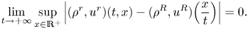
 \begin{equation} \lim_{t\rightarrow \infty}\sup_{x\in\mathbb{R^{+}}}\left|(\rho,u)(t,x)- (\rho^{R},u^{R})\Big(\frac{x}{t}\Big)\right|=0.\end{equation}
Remark 1.2 In the present article we consider only that the time-asymptotic state of the out-flow problem to one-dimensional compressible Navier-Stokes-Korteweg equations is rarefaction wave. The study of the stability of other wave pattern such as a viscous shock wave or the superposition of a rarefaction wave and a stationary wave will be carried out in other papers by the authors. Further, we try to give the complete classification of the asymptotic states of the outflow problem to the compressible Navier-Stokes-Korteweg equations as [Reference Kawashima and Zhu27, Reference Kawashima and Zhu28, Reference Matsumura36] for the compressible Navier-Stokes equation. Moreover, we should mention that the corresponding in-flow problem is surely more difficult, thus more interesting. Finally, we also mention that here we only focus on small perturbation of the initial data, in fact, it is interesting and plausible that we can consider the corresponding results for large perturbation. These are expected to be done in the forthcoming papers.
This article is follow-up study of [Reference Chen and Li8, Reference Chen, Li and Sheng9, Reference Li and Zhu35]. Now we give main ideas and arguments of the proof for theorem 1.1. Applying  $L^{2}$-energy method and some time-decay estimates in
  $L^{p}$-norm for the smoothed rarefaction wave as in [Reference Kawashima and Zhu28], we prove the asymptotic stability of the rarefaction wave in the case that the initial data are a small perturbation of the rarefaction wave. The key ingredient in the proof of theorem 1.1 is to deduce the a priori estimates. The main difficulties are as follows. The first one is the occurrence of the third order dispersion term. The second is that it is not easy to control the boundary terms
  $\varphi _{xx}(t,0)$,
  $\varphi _{xxx}(t,0)$ and
  $\psi _{xx}(t,0)$. To overcome the first difficulty, we need more regularities for the density and smooth rarefaction wave. We also note that the basic energy is obtained with the help of higher order estimates. For the second difficulty, we can introduce
  $\varphi _{xx}(t,0)^{2}$ by the second equation of (3.1) and integration by parts. Moreover, we can control
  $(\kappa \varphi _{xxx}(t,0)+ {\mu }\psi _{xx}(t,0)/{\rho (t,0)} )^{2}$ by
  $C \|\psi _{x}(t)\|_1^{2}$, which is derived by (3.1)
 $_2$ and lemma 2.2. These are the main novelty of the present paper.
The rest of the article is organized as follows. In § 2, we first review a smooth approximate rarefaction wave which tends to the rarefaction wave fan uniformly as the time  $t$ tends to infinity. Then we reformulate the original problem in terms of the perturbation variables in § 3. § 4 is the key part of this article, in which we will establish the a priori estimates by the elaborate energy estimates. Finally, we complete the proof of theorem 1.1 in § 5.
2. Smooth rarefaction wave
Since the rarefaction wave  $(\rho ^{R},u^{R})(x/t)$ is not smooth, we need to construct a smooth approximation of the rarefaction wave
  $(\rho ^{r},u^{r})(t,x)$. As [Reference Matsumura and Nishihara38], we start with the Riemann problem on
  $\mathbb {R}=(-\infty ,+\infty )$ for the typical Burgers equation:
 \begin{equation} w_{t}+ww_{x}=0,\end{equation}
with initial data
 \begin{equation} w(0,x)=w^{R}_{0}(x)=\begin{cases} w_{-}, & x<0\\ w_{+}, & x>0,\end{cases}\end{equation}
where  $w_\pm$ are given by
  $w_{-}=u_{b}+C(\rho _{-})>0$ and
  $w_{+}=u_{+}+C(\rho _{+})>0$, satisfying
  $w_-< w_+$. It is well known that the Riemann problem (2.1)–(2.2) has a unique rarefaction wave solution:
 \begin{eqnarray*} w^{R}\Big(\frac{x}{t}\Big)= \begin{cases} w_{-}, & x< w_{-}t, \\ \dfrac{x}{t}, & w_{-}t\leq x\leq w_{+}t, \\w_{+}, & x>w_{+}t.\end{cases} \end{eqnarray*}
Then we can define the functions  $\rho ^{R}(t,x)$ and
  $u^{R}(t,x)$ by
 \begin{align*} &\lambda_{2}(\rho^{R},u^{R})=u^{R}+C(\rho^{R})=w^{R}(1+t,x), \\&\frac{du^{R}}{d\rho^{R}}=\frac{C(\rho^{R})}{\rho^{R}}. \end{align*}
It is easy to check that  $\rho ^{R}(t,x)$ and
  $u^{R}(t,x)$ satisfy
 \[ \begin{cases}{\rho_{t}+(\rho u)_{x}=0,} \\ {(\rho u)_{t}+(\rho u^{2}+p(\rho))_{x}=0}\end{cases} \]
with
 \[ (\rho,u)(0,x)=\begin{cases} (\rho_{-},u_{b}), & x<0,\\ (\rho_{+},u_{+}), & x>0. \end{cases}\]
Now we approximate the rarefaction wave  $w^{R}(x/t)$ by the solution of the following Cauchy problem:
 \begin{align} \begin{cases}w_{t}+ww_{x}=0, \\w(0,x)=w^{r}_{0}(x)=\begin{cases} w_{-}, & x<0,\\ w_{-}+C_{q}\tilde{w}\int^{\varepsilon x}_{0}y^{q}e^{y}\textrm{d}y, & x\geq 0, \end{cases}\end{cases}\end{align}
where  $\tilde {w}=w_+-w_-$,
  $C_q>0$ is a constant satisfying:
  $C_q\int _0^{+\infty }z^{q}e^{-z}\textrm {d}z=1$ with
  $q\geq 10$ being a positive constant, and
  $\varepsilon \leq 1$ is a positive constant to be determined later. Then the properties of
  $w(t,x)$ can be summarised in the following lemma.
Lemma 2.1 (See [Reference Chen and Li8, Reference Huang, Matsumura and Shi24]) Let  $0< w_-< w_+$, then the Cauchy problem (2.3) admits a unique global smooth solution
  $w(t,x)$ satisfying:
(i)
 $w_{-}< w(t,x)< w_{+},\,\, w_{x}>0$, $x\geq 0,\,t\geq 0$.
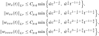
(ii) For any
$p (1\leq p\leq +\infty )$, there exists a constant $C_{p,q}>0$ such that for $t\geq 0$,
\begin{align*} \left\|w_{x}(t)\right\|_{L^{p}}& \leq C_{p,q}\min\Big\{\tilde{w}\varepsilon^{1-\frac{1}{p}},\ \tilde{w}^{\frac{1}{p}}t^{{-}1+\frac{1}{p}}\Big\},\\ \left\|w_{xx}(t)\right\|_{L^{p}}& \leq C_{p,q}\min\Big\{\tilde{w}\varepsilon^{2-\frac{1}{p}},\ \tilde{w}^{\frac{1}{q}}\varepsilon^{1-\frac{1}{p}+\frac{1}{q}}t^{{-}1+\frac{1}{q}}\Big\},\\ \left\|w_{xxx}(t)\right\|_{L^{p}}& \leq C_{p,q}\min\Big\{\tilde{w}\varepsilon^{3-\frac{1}{p}},\ \tilde{w}^{\frac{2}{q}}\varepsilon^{2-\frac{1}{p}+\frac{2}{q}}t^{{-}1+\frac{2}{q}}\Big\},\\ \left\|w_{xxxx}(t)\right\|_{L^{p}}& \leq C_{p,q}\min\Big\{\tilde{w}\varepsilon^{4-\frac{1}{p}},\ \tilde{w}^{\frac{3}{q}}\varepsilon^{3-\frac{1}{p}+\frac{3}{q}}t^{{-}1+\frac{3}{q}}\Big\}. \end{align*}(iii) When
$x\leq w_-t,$ it holds that
\[ w(t,x)-w_-{=}w_x(t,x)=w_{xx}(t,x)=w_{xxx}(t,x)=0. \](iv)
$\displaystyle \lim _{t\rightarrow +\infty }\sup _{x\in \mathbb {R}}\left |w(t, x)-w^{R}(t,x)\right |=0.$


Now, we define the smooth approximate rarefaction wave  $(\rho ^{r},u^{r})(t,x)$ of
  $(\rho ^{R},u^{R})(x/t)$ as follows:
 \begin{align*} &\lambda_{2}(\rho^{r},u^{r})=u^{R}+C(\rho^{r})=w(1+t,x), \\&\frac{du^{r}}{d\rho^{r}}=\frac{C(\rho^{r})}{\rho^{r}}. \end{align*}
Therefore, from lemma 2.1, we know that  $(\rho ^{r},u^{r})(t,x)$ has the following properties:
Lemma 2.2 Let 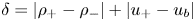 $\delta =|\rho _+-\rho _-|+|u_+-u_b|$, the smooth approximation
  $(\rho ^{r},u^{r})(t,x)$ of
  $(\rho ^{R},u^{R})$ has the following properties:
(i)
$u_x^{r}\geq 0,\quad |u_x^{r}|\leq C\varepsilon ,\quad \forall \,t\geq 0,\,x\geq 0$.(ii) For any
$p$ with $1\leq p\leq +\infty$, there exists a constant $C_{p,q}>0$ such that
\begin{align*} \left\|\left(\rho_x^{r}, u_x^{r}\right)(t)\right\|_{L^{p}}&\leq C_{p,q}\min\Big\{\delta\varepsilon^{1-\frac{1}{p}},\ \delta^{\frac{1}{p}}(1+t)^{{-}1+\frac{1}{p}}\Big\},\\ \left\|\left(\rho_{xx}^{r}, u_{xx}^{r}\right)(t)\right\|_{L^{p}}&\leq C_{p,q}\min\Big\{\delta\varepsilon^{2-\frac{1}{p}},\ \delta^{\frac{1}{q}}\varepsilon^{1-\frac{1}{p}+\frac{1}{q}}(1+t)^{{-}1+\frac{1}{q}}\Big\},\\ \left\|\left(\rho_{xxx}^{r}, u_{xxx}^{r}\right)(t)\right\|_{L^{p}}&\leq C_{p,q}\min\Big\{\delta\varepsilon^{3-\frac{1}{p}},\ \delta^{\frac{2}{q}}\varepsilon^{2-\frac{1}{p}+\frac{2}{q}}(1+t)^{{-}1+\frac{2}{q}}\Big\},\\ \left\|\left(\rho_{xxxx}^{r}, u_{xxxx}^{r}\right)(t)\right\|_{L^{p}}&\leq C_{p,q}\min\Big\{\delta\varepsilon^{4-\frac{1}{p}},\ \delta^{\frac{3}{q}}\varepsilon^{3-\frac{1}{p}+\frac{3}{q}}(1+t)^{{-}1+\frac{3}{q}}\Big\}. \end{align*}(iii)
$(\rho ^{r},u^{r})(t,x)\Big |_{x\leq \lambda _2(\rho _-,u_b)t}$ $=(v_-,u_-), \frac {\partial ^{j}}{\partial x^{j}}(\rho ^{r},u^{r})(t,x)\Big |_{x\leq \lambda _2(\rho _-,u_b)t}=0, j=1,2,3.$(iv)
$\displaystyle \lim _{t\rightarrow +\infty }\sup _{x\in \mathbb {R}^{+}}\left |(\rho ^{r},u^{r})(t,x)-(\rho ^{R}, u^{R})\Big (\frac {x}{t}\Big )\right |=0.$


3. Reformulation of the problem
Since it is convenient to regard the solution  $(\rho ,u)$ as the perturbation of
  $(\rho ^{r},u^{r})$, we are going to reformulate the original problem in terms of the perturbation variables in this section. First, we define
 \[ \varphi(t,x)=\rho(t,x)-\rho^{r}(t,x),~\psi(t,x)=u(t,x)-u^{r}(t,x). \]
Then, the original problem (1.1)–(1.4) can be rewritten as
 \begin{align} \left\{\begin{array}{@{}l}{\varphi_{t}+\rho\psi_{x}+u\varphi_{x}=f,} \\ {\rho(\psi_{t}+u\psi _{x})+p'(\rho)\varphi_{x}=\mu\psi_{xx}+\kappa\rho\varphi_{xxx}+g}\end{array}\right. \end{align}
with the initial boundary conditions:
 \begin{align} \left\{\begin{array}{@{}l} (\varphi, \psi)(0,x)=(\rho_{0}(x)-\rho^{r}(0,x),u_{0}(x)-u^{r}(0,x),\\ \psi(t,0)=0,\\ \varphi_{x}(t,0)=\rho_x(t,0)-\rho_x^{r}(t,0)=0, \end{array}\right. \end{align}
where
 \begin{equation} f={-}u^{r}_{x}\varphi-\rho^{r}_{x}\psi,\end{equation}
and
 \begin{equation} g=\mu u^{r}_{xx}+\kappa\rho\rho^{r}_{xxx}+\frac{p'(\rho^{r})}{p^{r}}\rho^{r}_{x}\varphi-[p'(\rho)-p'(\rho^{r})]\rho^{r}_{x}-\rho\psi u^{r}_{x}.\end{equation}
 Therefore, we are now in a position to restate our main results in terms of the perturbed variable  $(\varphi ,\psi )(t,x )$ as follows.
Theorem 3.1 Suppose that all the assumptions of theorem 1.1 are met. Then there exists a unique global solution  $(\varphi ,\psi )(t,x )$ to problem (3.1)–(3.2), satisfying
 \begin{align*} &\varphi,\psi\in C([0,\infty); L^{2}(\mathbb{R^{+}})),\\ &\varphi_{x}, \varphi_{xx}, \psi_{x}\in C([0,\infty); L^{2}(\mathbb{R^{+}}))\cap L^{2}([0,\infty); L^{2}(\mathbb{R^{+}})), \\ &\varphi_{xxx}, \psi_{xx}\in L^{2}([0,\infty); L^{2}(\mathbb{R^{+}})), \end{align*}
and
 \[ \lim_{t\rightarrow \infty}\sup_{x\in\mathbb{R^{+}}}|(\varphi,\psi)(t,x)|=0. \]
 To prove this theorem, we shall employ the standard continuation argument based on a local existence theorem in the following lemma and on a priori estimates stated in the following proposition. First, the local existence of the solution  $(\varphi ,\psi )$ to the initial-boundary value problem (3.1)–(3.2) is proved by the standard method, for example, the dual argument and iteration technique. For details, we refer [Reference Hattori and Li17, Reference Hattori and Li18, Reference Kotschote31, Reference Tsyganov45].
Lemma 3.2 Local existence Assume that the conditions in theorem 1.1 hold. Then there exists a positive constant  $T_0$ such that the initial-boundary value problem (3.1)–(3.2) has a unique strong solution
  $(\varphi ,\psi )(t,x)$ that has the following properties:
 \begin{align*} & \varphi(t,x)\in C([0,T_{0}];H^{2}(\mathbb{R}^{+})), \psi(t,x)\in C([0,T_{0}]; H^{1}(\mathbb{R}^{+})),\\ & \varphi_{x}(t,x)\in L^{2}([0,T_{0}];H^{2}(\mathbb{R}^{+})) ,~\psi_{x}(t,x)\in L^{2}([0,T_{0}];H^{1}(\mathbb{R}^{+})),\\ & \inf_{t\in[0,T_0],x\in\mathbb{R}^{+}} \rho(t,x) >0. \end{align*}
Next, we prove the following a priori estimates in Sobolev spaces, which are stated in proposition 3.3.
Proposition 3.3 Let  $(\varphi ,\psi )$ be a solution to the initial-boundary value problem (3.1)–(3.2) in a time interval
  $[0,T]$, which has same regularities as in lemma 3.2. Then there exist constants
  $\varepsilon _1>0$ and
  $C>0$ such that if
 \begin{align} N(T) := \displaystyle\sup_{t\in[0, T]}[\|\varphi(t)\|_2 +\|\psi(t)\|_1]\le \varepsilon_1, \end{align}
then the following estimate holds for any  $t\in [0,T]$
 \begin{align} & \|\varphi(t)\|_{2}^{2}+\|\psi(t)\|_1^{2} +\int_0^{t}\left(\|\varphi_{x}(\tau)\|_{2}^{2}+\|\psi_{x}(\tau)\|_{1}^{2} +|(\varphi,\varphi_{xx})(\tau,0)|^{2}\right)d\tau\nonumber\\ &\quad \le C(\|\varphi_{0}\|_{2}^{2}+\|\psi_{0}\|_1^{2}+\varepsilon^{\frac 18}). \end{align}
4. A priori estimate
This section is devoted to the derivation of a priori estimates for the unknown function  $(\varphi ,\psi )(t,x)$ and their derivatives, we then show that proposition 3.3 is valid. To derive these a priori estimates, we assume that there exists a strong solution
  $(\varphi ,\psi )(t,x)$ to problem (3.1)–(3.2), such that
 \begin{align*} & \varphi(t,x)\in C([0,T];H^{2}(\mathbb{R}^{+})),\ \psi(t,x)\in C([0,T]; H^{1}(\mathbb{R}^{+})),\\ & \varphi_{x}(t,x)\in L^{2}([0,T];H^{2}(\mathbb{R}^{+})) , \psi_{x}(t,x)\in L^{2}([0,T];H^{1}(\mathbb{R}^{+})),\\ &\inf_{(t,x)\in [0,T]\times\mathbb{R}^{+}}(\varphi+\rho^{r})(t,x)>0 \end{align*}
for any  $T>0$. Indeed, we may assume that
  $(\varphi ,\psi )(t,x)$ is a classical solution from the standard mollifier arguments. From (3.5), one can see easily that there exist two positive constants
  $c$ and
  $C$ such that
 \begin{align} 0< c\leq \rho\leq C,~|u|\leq C~~\textrm{for}~t\in [0,T], \end{align}
since  $\rho ^{r} \geq c>0$ for a positive constant
  $c$. To this end, we introduce
 \[ \Phi(\rho,\rho^{r})=\int^{\rho}_{\rho^{r}}\frac{p(\eta)-p(\rho^{r})}{\eta^{2}}d\eta, \]
combining this with (4.1) yields
 \begin{align} c\varphi^{2}\leq\Phi(\rho,\rho^{r})\leq C\varphi^{2}. \end{align}
Next, from (3.1), the straightforward but tedious computations give
 \begin{align} &\Big [\rho\Big(\frac{1}{2}\psi^{2}+\Phi(\rho,\rho^{r})\Big)\Big]_{t}+\Big[\rho u\Big(\frac{1}{2}\psi^{2}+\Phi(\rho,\rho^{r})) +(p(\rho)-p(\rho^{r})\Big)\psi-\mu\psi\psi_{x}\Big]_{x} \nonumber\\ = \,\,&-\mu \psi^{2}_{x}-[\rho \psi^{2}+p(\rho)-p(\rho^{r})-p'(\rho)\varphi]u^{r}_{x} +\kappa\rho\varphi_{xxx}\psi+\mu u^{r}_{xx}\psi+\kappa\rho\rho^{r}_{xxx}\psi. \end{align}
Moreover from (3.1) $_1$, we also have
 \begin{align*} \kappa\rho\varphi_{xxx}\psi &=\kappa(\rho\varphi_{xx}\psi)_{x}-\kappa(\rho\psi)_{x}\varphi_{xx}\nonumber\\ &=\kappa(\rho\varphi_{xx}\psi)_{x}+\kappa\varphi_{xx}(\varphi_{t}+u^{r}\varphi_{x}+u^{r}_{x}\varphi)\nonumber\\ &=\kappa(\rho\varphi_{xx}\psi)_{x}+\kappa(\varphi_{x}\varphi_{t})_{x}-\Big(\frac{\kappa}{2}\varphi^{2}_{x}\Big)_{t} +\frac{\kappa}{2}(\varphi^{2}_{x}u^{r})_{x} -\frac{\kappa}{2}u^{r}_{x}\varphi^{2}_{x}+\kappa u^{r}_{x}\varphi\varphi_{xx}\nonumber\\ &=\left(\kappa\rho\varphi_{xx}\psi+\kappa\varphi_{x}\varphi_{t}+\frac{\kappa}{2}u^{r}\varphi^{2}_{x}+\kappa u^{r}_{x}\varphi\varphi_{x}\right)_{x}\\ &\quad -\frac{\kappa}{2}(\varphi^{2}_{x})_{t}-\frac{3\kappa}{2}u^{r}_{x}\varphi^{2}_{x}-\kappa u^{r}_{xx}\varphi\varphi_{x}, \end{align*}
which together with (4.3) implies
 \begin{align} &\Big[\rho\Big(\frac{1}{2}\psi^{2}+\Phi(\rho,\rho^{r})\Big)+\frac{\kappa}{2}\varphi^{2}_{x}\Big]_{t} +R_{1x} +R_2\notag\\ &\quad =\mu u^{r}_{xx}\psi+\kappa\rho\rho_{xxx}^{r}\psi-\frac{3\kappa}{2}u^{r}_{x}\varphi^{2}_{x}-\kappa u^{r}_{xx}\varphi\varphi_{x}, \end{align}
here
 \begin{align*} R_1&=\rho u\left(\frac{1}{2}\psi^{2}+\Phi(\rho,\rho^{r})\right)+(p(\rho)-p(\rho^{r}))\psi-\mu\psi\psi_{x} \\ &\quad -\kappa\rho\varphi_{xx}\psi-\kappa\varphi_{x}\varphi_{t} -\frac{\kappa}{2}u^{r}\varphi^{2}_{x}-\kappa u^{r}_{x}\varphi\varphi_{x}, \end{align*}
and
 \begin{eqnarray*} R_2=[\rho\psi^{2}+p(\rho)+p(\rho^{r})-p'(\rho)\varphi]u^{r}_{x}+\mu\psi^{2}_{x}. \end{eqnarray*}
Then we arrive at
Lemma 4.1 Assume that  $(\varphi ,\psi )(t,x)$ is a solution to
  $($3.1
 $)$–
$)$– $($3.2
 $)$, satisfying the conditions in proposition 3.3, then the following estimate holds
 \begin{align} &\|\varphi(t)\|^{2}+\|\psi(t)\|^{2}+\|\varphi_x(t)\|^{2} +\int_0^{t}(\|\psi_x(\tau)\|^{2}+\varphi(\tau,0)^{2})d\tau\nonumber\\ &\quad \leq C(\|\varphi_0\|_1^{2}+\|\psi_0\|^{2}+ C\varepsilon^{\frac 18})+ C(\varepsilon^{\frac 13}+\varepsilon)\int_0^{t}\|\varphi_x(\tau )\|^{2}d\tau \end{align}
for all  $t\in [0,T]$.
Proof. Integrating (4.4) with respect to  $x$ over
  $(0,\infty )$ yields
 \begin{align} &\frac{\textrm{d}}{\textrm{d}t}\int_0^{\infty}\left(\frac{1}{2}\rho\psi^{2}+\rho\Phi\right)\textrm{d}x +\Big.R_{1}\Big|_{x=0}+\int_{0}^{\infty}R_{2}\textrm{d}x\nonumber\\ &\quad = \int_{0}^{\infty}(\mu u^{r}_{xx}\psi+\kappa\rho\rho_{xxx}^{r}\psi-\frac{3\kappa}{2}u^{r}_{x}\varphi^{2}_{x}-\kappa u^{r}_{xx}\varphi\varphi_{x})\textrm{d}x. \end{align}
First, noting (4.1) and using (4.2), we easily obtain
 \begin{align} \int_{0}^{\infty}\left(\frac{1}{2}\rho\psi^{2}+\rho\Phi\right)\textrm{d}x \ge c(\|\varphi\|^{2}+\|\psi\|^{2}), \end{align}
and
 \begin{align} R_1|_{x=0}={-}\rho u\Phi(\rho,\rho^{r})|_{x=0} \ge c\varphi(t,0)^{2} \end{align}
with the help of  $\psi (t,0)=0=\varphi _x(t,0)$ and
  $u_{b}<0$. Similarly, we have
 \begin{align} R_2\leq C(\|\sqrt{u^{r}_{x}}\varphi\|^{2}+\|\sqrt{u^{r}_{x}}\psi\|^{2}+\|\sqrt{u^{r}_{x}}\varphi_x\|^{2}+\|\psi_x\|^{2}). \end{align}
Further, combining (4.6)–(4.9) and using (4.1), we have
 \begin{align} &\frac{\textrm{d}}{\textrm{d}t}\int_0^{\infty}(\varphi^{2}+\psi^{2}+\varphi_x^{2})\textrm{d}x +\|\sqrt{u^{r}_{x}}\varphi\|^{2}+\|\sqrt{u^{r}_{x}}\psi\|^{2}\nonumber\\ &\quad +\|\psi_{x}\|^{2}+\|\sqrt{u^{r}_{x}}\varphi_x\|^{2}+\varphi(t,0)^{2}\nonumber\\ &\quad \leq C\Big|\int_{0}^{\infty} u^{r}_{xx}\psi \textrm{d}x\Big|+C\Big|\int_{0}^{\infty}\rho_{xxx}^{r}\psi \textrm{d}x\Big|+C\Big|\int_{0}^{\infty}u^{r}_{x}\varphi^{2}_{x}\textrm{d}x\Big|+C\Big|\int_{0}^{\infty} u^{r}_{xx}\varphi\varphi_{x}\textrm{d}x\Big|. \end{align}
Now let us estimate the terms on the right-hand side of (4.10). First, we employ Hölder inequality, the Sobolev inequality
 \begin{align} \|f\|_{L^{\infty}}\leq\sqrt{2}\|f\|^{\frac{1}{2}}\|f_{x}\|^{\frac{1}{2}} \end{align}
for any  $f\in H^{1}(\mathbb {R}^{+})$, lemma 2.2 and Young inequality to obtain
 \begin{align} \Big|\int_0^{\infty} u^{r}_{xx}\psi \textrm{d}x\Big|&\leq \|\psi\|_{L^{\infty}}\|u^{r}_{xx}\|_{L^{1}} \leq C\|\psi\|^{\frac{1}{2}}\|\psi_{x}\|^{\frac{1}{2}}\|u^{r}_{xx}\|_{L^{1}}\nonumber\\ & \leq \frac{1}{4}\|\psi_{x}\|^{2}+C\|\psi\|^{\frac{2}{3}}\|u^{r}_{xx}\|_{L^{1}}^{\frac{4}{3}}\nonumber\\ & \leq \frac{1}{4}\|\psi_{x}\|^{2}+C\|\psi\|^{\frac{2}{3}}\|u^{r}_{xx}\|_{L^{1}}^{\frac{1}{6}}\|u^{r}_{xx}\|_{L^{1}}^{\frac{7}{6}}\nonumber\\ & \leq \frac{1}{4}\|\psi_{x}\|^{2}+C\varepsilon^{\frac{1}{6}}(1+t)^{-\frac{21}{20}}\|\psi\|^{\frac{2}{3}}\nonumber\\ & \leq \frac{1}{4}\|\psi_{x}\|^{2}+C\varepsilon^{\frac{1}{4}}(1+t)^{-\frac{21}{20}}\|\psi\|^{2} +C\varepsilon^{\frac{1}{8}}(1+t)^{-\frac{21}{20}}. \end{align}
Similarly, we have
 \begin{align} \Big|\int_0^{\infty} \rho^{r}_{xxx}\psi \textrm{d}x\Big|&\leq C\|\psi\|^{\frac{1}{2}}\|\psi_{x}\|^{\frac{1}{2}}\|\rho^{r}_{xxx}\|_{L^{1}}\nonumber\\ & \leq \frac{1}{4}\|\psi_{x}\|^{2}+C\|\psi\|^{\frac{2}{3}}\|\rho^{r}_{xxx}\|_{L^{1}}^{\frac{4}{3}}\nonumber\\ & \leq \frac{1}{4}\|\psi_{x}\|^{2}+C\varepsilon^{\frac{1}{6}}(1+t)^{-\frac{16}{15}}\|\psi\|^{\frac{2}{3}}\nonumber\\ & \leq \frac{1}{4}\|\psi_{x}\|^{2}+C\varepsilon^{\frac{1}{4}}(1+t)^{-\frac{11}{10}}\|\psi\|^{2} +C\varepsilon^{\frac{1}{8}}(1+t)^{-\frac{21}{20}}. \end{align}
Next, from lemma 2.2, it is easy to obtain
 \begin{align} \Big|\int_0^{\infty} u^{r}_{x}\varphi^{2}_{x}\textrm{d}x\Big|\leq C\varepsilon\|\varphi_{x}\|^{2}. \end{align}
Finally, using Hölder inequality, lemma 2.2 and Young inequality, we have
 \begin{align} \Big|\int_0^{\infty} u^{r}_{xx}\varphi\varphi_{x}\textrm{d}x\Big|& \leq C\|u^{r}_{xx}\|_{L^{\infty}}^{\frac 16}\|u^{r}_{xx}\|_{L^{\infty}}^{\frac 56}\|\varphi\|\|\varphi_{x}\|\nonumber\\ & \leq C\varepsilon^{\frac{1}{3}}(1+t)^{-\frac{3}{4}}\|\varphi\|\|\varphi_{x}\|\nonumber\\ & \leq C\varepsilon^{\frac{1}{3}}\|\varphi_{x}\|^{2} +C\varepsilon^{\frac{1}{3}}(1+t)^{-\frac 32}\|\varphi\|^{2}. \end{align}
Therefore, combining (4.10), (4.12)–(4.14) and (4.15), and integrating the resultant inequality with respect to  $t$, then implies (4.5) provided that
  $C\varepsilon ^{\frac {1}{4}}<\frac 14$ and
  $C\varepsilon ^{\frac {1}{3}}<\frac 14$. This completes the proof of lemma 4.1.
Next, we derive the estimate for  $\varphi _x$ and
  $\varphi _{xx}$.
Lemma 4.2 Assume that  $(\varphi ,\psi )(t,x)$ is a solution to
  $($3.1
 $)$–
$)$– $($3.2
 $)$, satisfying the conditions in proposition 3.3, then the following estimate holds
 \begin{align} \|\varphi_{x}\|_1^{2}\le C(\|\varphi_0\|_1^{2}+\|\psi_0\|^{2}+ C\varepsilon^{\frac 18}) \end{align}
for all  $t\in [0,T]$.
Proof. We first differentiate formally (3.1) $_1$ in
  $x$ to obtain
 \begin{align} \varphi_{tx}+u\varphi_{xx}+\rho\psi_{xx}=f_{x}-\rho_{x}^{r}\psi_{x}-u_{x}^{r}\varphi_{x}-2\varphi_{x}\psi_{x}. \end{align}
Then multiplying above equation by  $\frac {1}{\rho ^{2}}\varphi _{x}$, and integrating the resulting equality with respect to
  $x$ over
  $\mathbb {R}^{+}$ by parts, one has
 \begin{align} \frac{1}{2}\frac{\textrm{d}}{\textrm{d}t}\int_0^{\infty}\frac{\varphi_{x}^{2}}{\rho^{2}}\textrm{d}x+\int_0^{\infty}\frac{1}{\rho}\psi_{xx}\varphi_{x}\textrm{d}x=\int_0^{\infty} f_{1}\frac{\varphi_{x}}{\rho^{2}}\textrm{d}x, \end{align}
with the help of  $\varphi _x(t,0)=0$ and (1.1)
 $_1$, here
 \[ f_{1}=f_{x}-\rho^{r}_{x}\psi_{x}-\frac 12\varphi_{x}\psi_{x}+\frac 12u_{x}^{r}\varphi_{x}. \]
Moreover, multiplying (3.1) $_2$ by
  $\frac {1}{\rho }\varphi _{x}$, and integrating the resulting equality with respect to
  $x$ over
  $\mathbb {R}^{+}$ by parts, and using
  $\psi (t,0)=\varphi _x(t,0)=0$ and (3.1)
 $_1$, we have
 \begin{align*} &\frac{\textrm{d}}{\textrm{d}t}\int_0^{\infty}\varphi_{x}\psi \textrm{d}x+\int_0^{\infty}\frac{p'(\rho)}{\rho}\varphi_{x}^{2}\textrm{d}x+\kappa\int_0^{\infty}\varphi_{xx}^{2}\textrm{d}x\\ &\quad = \int_0^{\infty}\frac{\mu}{\rho}\psi_{xx}\varphi_{x}\textrm{d}x +\int_0^{\infty}\frac{g}{\rho}\varphi_{x}\textrm{d}x+\int_0^{\infty}\psi_{x}(\rho\psi_{x}+u\varphi_{x}-f)\textrm{d}x \end{align*}
which together with (4.18) yields
 \begin{align} &\frac{\textrm{d}}{\textrm{d}t}\int_0^{\infty}\Big(\frac{\mu}{2\rho^{2}}\varphi_{x}^{2}+\psi\varphi_{x}\Big) \textrm{d}x +\int_0^{\infty}\frac{p'(\rho)}{\rho}\varphi_{x}^{2}+\kappa\int_0^{\infty}\varphi_{xx}^{2}\textrm{d}x\nonumber\\ = \,\, &\int_0^{\infty}\frac{\mu}{\rho^{2}}f_{1}\varphi_{x}\textrm{d}x+\int_0^{\infty}\frac{g}{\rho}\varphi_{x}\textrm{d}x +\int_0^{\infty}\psi_{x}(\rho\psi_{x}+u\varphi_{x}-f)\textrm{d}x. \end{align}
Further, using (4.1), we have
 \begin{align} \frac{\textrm{d}}{\textrm{d}t}\int_0^{\infty}(\varphi_{x}^{2}+\psi\varphi_{x}) \textrm{d}x +\|\varphi_{x}(t)\|^{2}+\|\varphi_{xx}(t)\|^{2}\leq C\|\psi_{x}(t)\|^{2}+C\sum_{i=1}^{5}I_i, \end{align}
where
 \begin{eqnarray*} I_1&=&\Big|\int_0^{\infty}\varphi_x\psi_{x}\textrm{d}x\Big|+\Big|\int_0^{\infty}\varphi_x^{2}\psi_{x}\textrm{d}x\Big|,\\ I_2&=&\Big|\int_0^{\infty} u_{x}^{r}\varphi_x^{2}\textrm{d}x\Big|+\Big|\int_0^{\infty} \rho_{x}^{r}\varphi_x\psi_{x}\textrm{d}x\Big|,\\ I_3&=&\Big|\int_0^{\infty} u_{xx}^{r}\varphi\varphi_{x}\textrm{d}x\Big|+\Big|\int_0^{\infty}|\rho_{xx}^{r}\psi\varphi_{x}\textrm{d}x\Big|,\\ I_4&=&\Big|\int_0^{\infty} u_{x}^{r}\varphi\psi_{x}\textrm{d}x\Big|+\Big|\int_0^{\infty}\rho_{x}^{r}\psi\psi_{x}\textrm{d}x\Big|+\Big|\int_0^{\infty} u_{x}^{r}\psi\varphi_{x}\textrm{d}x\Big|+\Big|\int_0^{\infty}\rho_{x}^{r}\varphi\varphi_{x}\textrm{d}x\Big|, \end{eqnarray*}
and
 \begin{eqnarray*} I_5&=&\Big|\int_0^{\infty} u_{xx}^{r}\varphi_{x}\textrm{d}x\Big|+\Big|\int_0^{\infty}\rho_{xxx}^{r}\varphi_{x}\textrm{d}x\Big|. \end{eqnarray*}
 In the following, let us estimate  $I_1-I_4$ and
  $I_5$. First, from Young inequality and (3.5), it is easy to obtain
 \begin{align} I_1 & \leq C\|\psi_{x}\|^{2}+\frac 18\|\varphi_{x}\|^{2}+C\|\varphi_{x}\|_{L^{\infty}}(\|\varphi_{x}\|^{2}+\|\psi_{x}\|^{2})\nonumber\\ & \leq C\|\psi_{x}(t)\|^{2}+\frac 18\|\varphi_{x}(t)\|^{2}+C\varepsilon_1\|(\varphi_{x},\psi_{x})(t)\|^{2}. \end{align}
Similar as (4.14) and (4.15), we conclude
 \begin{align} I_2\leq C\varepsilon(\|\varphi_{x}(t)\|^{2}+\|\psi_{x}(t)\|^{2}), \end{align}
and
 \begin{align} I_3\leq C\varepsilon^{\frac{1}{3}}\|\varphi_{x}\|^{2} +C\varepsilon^{\frac{1}{3}}(1+t)^{-\frac{3}{2}}\|(\varphi,\psi)(t)\|^{2}. \end{align}
Finally, using lemma 2.2, Hölder inequality and Young inequality, we have
 \begin{align} I_4 & \leq C\|u^{r}_{x}\|^{\frac{1}{4}}_{L^{\infty}}\|u^{r}_{x}\|^{\frac{3}{4}}_{L^{\infty}}(\|\varphi\|\|\psi_{x}\| +\|\psi\|\|\varphi_{x}\|)\notag\\ &\quad +C\|\rho^{r}_{x}\|^{\frac{1}{4}}_{L^{\infty}}\|\rho^{r}_{x}\|^{\frac{3}{4}}_{L^{\infty}}(\|\varphi\|\|\varphi_{x}\| +\|\psi\|\|\psi_{x}\|)\nonumber\\ & \leq C\varepsilon^{\frac{1}{4}}(\|\varphi_{x}(t)\|^{2}+\|\psi_{x}(t)\|^{2}) +C\varepsilon^{\frac{1}4}(1+t)^{-\frac{3}{2}}\|(\varphi,\psi)(t)\|^{2}, \end{align}
and
 \begin{align} I_5&\leq \frac 18\|\varphi_{x}\|^{2}+ C\|u^{r}_{xx}\|^{2}+C\|\rho^{r}_{xxx}\|^{2}\notag\\ &\leq\frac 18\|\varphi_{x}(t)\|^{2} +C\varepsilon^{\frac{1}5}(1+t)^{-\frac 95}+C\varepsilon^{\frac{2}5}(1+t)^{-\frac 85}. \end{align}
Therefore, insertion of (4.21)–(4.25) into (4.20), and integrating the resultant inequality with respect to  $t$ and using (4.5), yields (4.16) if
  $C\varepsilon ^{\frac {1}{4}}<\frac 14$ and
  $C\varepsilon ^{\frac {1}{3}}<\frac 14$, and
  $\varepsilon _1$ is assumed sufficiently small. This completes the proof of lemma 4.2.
With lemmas 4.1 and 4.2 in hand, we can show the fundamental energy estimate.
Corollary 4.3 Assume that  $(\varphi ,\psi )(t,x)$ is a solution to
  $($3.1
 $)$–
$)$– $($3.2
 $)$, satisfying the conditions in proposition 3.3, then it holds that
 \begin{align} &\|\varphi(t)\|_1^{2}+\|\psi(t)\|^{2} +\int_0^{t}(\|\psi_x(\tau)\|^{2}+\|\varphi_x(t)\|_1^{2}+\varphi(\tau,0)^{2})d\tau\nonumber\\ &\quad \leq C(\|\varphi_0\|_1^{2}+\|\psi_0\|^{2}+ \varepsilon^{\frac 18}) \end{align}
for any  $t\in [0,T]$.
Next, let us derive estimates for the derivatives of unknowns, i.e.,  $\varphi _{xx}$ and
  $\psi _{x}$.
Lemma 4.4 Assume that  $(\varphi ,\psi )(t,x)$ is a solution to
  $($3.1
 $)$–
$)$– $($3.2
 $)$, satisfying the conditions in proposition 3.3, then it holds
 \begin{align} &\|\psi_x(t)\|^{2}+ \|\varphi_{xx}(t)\|^{2}+\int_0^{t}(\|\psi_{xx}(\tau)\|^{2} +\varphi_{xx}(\tau,0)^{2})d\tau\nonumber\\ &\quad \leq C(\|\varphi_0\|_2^{2}+\|\psi_0\|_1^{2}+\varepsilon^{\frac 18}) +C(\varepsilon^{\frac{1}{3}}+\varepsilon_1)\int_0^{t}\|\varphi_{xxx}(\tau)\|^{2}d\tau \end{align}
for all  $t\in [0,T]$.
Proof. Multiplying (3.1) $_2$ by
  $-\psi _{xx}$ and integrating the resultant equal over
  $\mathbb {R}^{+}$ with respect to
  $x$, we have
 \begin{align} &\frac{1}{2}\frac{\textrm{d}}{\textrm{d}t}\int_0^{\infty}\rho\psi_{x}^{2}\textrm{d}x+\mu\int_0^{\infty}\psi_{xx}^{2}\textrm{d}x \notag\\ &\quad = -\kappa\int_0^{\infty}(\rho\varphi_{xxx}\psi_{xx}+\rho_{x}\psi_{x}\varphi_{xxx})\textrm{d}x +\int_0^{\infty}\rho u\psi_{x}\psi_{xx}\textrm{d}x\nonumber\\ &\qquad +\int_0^{\infty} p'(\rho)\varphi_{x}\psi_{xx}\textrm{d}x-\int_0^{\infty} g\psi_{xx}\textrm{d}x\nonumber\\ &\qquad -\int_{0}^{\infty}\rho_{x}\psi_{x}\Big[\frac{g}{\rho}+\frac{\mu}{\rho}\psi_{xx} -\frac{p'(\rho)}{\rho}\varphi_{x}-u\psi_{x}\Big]\textrm{d}x\nonumber\\ &\qquad -\frac{1}{2}\int_0^{\infty}\psi_{x}^{2}(\rho\psi_{x}+u\varphi_{x}+\rho u_x^{r}+u\rho_{x}^{r})\textrm{d}x, \end{align}
here we have used
 \begin{align*} -\int_0^{\infty}\rho \psi_{t}\psi_{xx}\textrm{d}x&=-\rho \psi_{t}\psi_{x}\mid_{0}^{\infty}+ \frac{1}{2}\frac{\textrm{d}}{\textrm{d}t}\int_0^{\infty}\rho\psi_{x}^{2}\textrm{d}x\\ &\quad - \frac{1}{2}\int_0^{\infty}\rho_{t}\psi_{x}^{2}\textrm{d}x+ \int_0^{\infty}\rho_{x}\psi_{t}\psi_{x}\textrm{d}x \nonumber \\ &=\frac{1}{2}\frac{\textrm{d}}{\textrm{d}t}\int_0^{\infty}\rho\psi_{x}^{2}\textrm{d}x-\frac{1}{2}\int_0^{\infty}\rho_{t}\psi_{x}^{2}\textrm{d}x + \int_{0}^{\infty}\rho_{x}\psi_{t}\psi_{x}\textrm{d}x \end{align*}
and  $\psi _t(t,0)=0$, (1.1)
 $_1$ and (3.1)
 $_2$. On the other hand, note that
 \[ \psi_{t}\varphi_{xx}=(\varphi_{xx}\psi)_{t}-(\psi\varphi_{tx})_{x}+\psi_{x}\varphi_{tx}, \]
and
 \[ 2\int_0^{\infty}\varphi_{xxx}\varphi_{xx}\textrm{d}x={-}\varphi_{xx}(t,0)^{2}, \]
then multiplying (3.1) $_2$ by
  $-({2u_{b}}/{\rho })\varphi _{xx}$, and integrating the resulting equality over
  $\mathbb {R}^{+}$ with respect to
  $x$, and using (4.17) and
  $\varphi _{tx}(t,0)=0$, we have
 \begin{align*} &\frac{\textrm{d}}{\textrm{d}t}\int_0^{\infty}-2u_{b}\psi\varphi_{xx}\textrm{d}x-\kappa u_{b}\varphi_{xx}(t,0)^{2}\\ &\quad = -2u_{b}\int_0^{\infty}\Big[\frac{g}{\rho} +\frac{\mu}{\rho}\psi_{xx}-\frac{p'(\rho)}{\rho}\varphi_{x}\Big]\varphi_{xx}\textrm{d}x\nonumber\\ &\qquad +2u_{b}\int_0^{\infty}\psi_{x}(f_{x}-\rho\psi_{xx}-\rho_{x}^{r}\psi_{x}-u_{x}^{r}\varphi_{x}-2\varphi_x\psi_x)\textrm{d}x, \end{align*}
which together with (4.28) yields
 \begin{align} &\frac{\textrm{d}}{\textrm{d}t}\int_0^{\infty}\left( \frac{1}{2}\rho\psi_{x}^{2}-2u_{b}\psi\varphi_{xx}\right)\textrm{d}x+\mu\int_{0}^{\infty}\psi_{xx}^{2}\textrm{d}x -\kappa u_{b}\varphi_{xx}(t,0)^{2}\nonumber\\ &\quad = -\kappa\int_0^{\infty}(\rho\varphi_{xxx}\psi_{xx}+\rho_{x}\psi_{x}\varphi_{xxx})\textrm{d}x+\int_0^{\infty}[\rho u\psi_{x}+ p'(\rho)\varphi_{x}-2u_b\psi_{x}]\psi_{xx}\textrm{d}x\nonumber\\ &\qquad -2u_{b}\int_0^{\infty}\left[\frac{\mu}{\rho}\psi_{xx}-\frac{p'(\rho)}{\rho}\varphi_{x}\right]\varphi_{xx}\textrm{d}x -\frac{1}{2}\int_0^{\infty}\psi_{x}^{2}(\rho\psi_{x}+u\varphi_{x}+\rho u^{r}+u\rho_{x}^{r})\textrm{d}x\nonumber\\ &\qquad -\int_0^{\infty} g\psi_{xx}\textrm{d}x-2u_{b}\int_0^{\infty}\frac{g}{\rho}\varphi_{xx}\textrm{d}x\notag\\ &\qquad -\int_{0}^{\infty}\rho_{x}\psi_{x} \left[\frac{g}{\rho} +\frac{\mu}{\rho}\psi_{xx}-\frac{p'(\rho)}{\rho}\varphi_{x}-u\psi_{x}\right]\textrm{d}x\nonumber\\ &\qquad +2u_{b}\int_0^{\infty}\psi_{x}(f_{x}-\rho_{x}^{r}\psi_{x} -u_{x}^{r}\varphi_{x}-2\varphi_x\psi_x)\textrm{d}x. \end{align}
First, from (4.1) and the Young inequality, one has
 \begin{align} \int_0^{\infty}[\rho u\psi_{x}+ p'(\rho)\varphi_{x}-2u_b\psi_{x}]\psi_{xx}\textrm{d}x \le \frac\mu 8\|\psi_{xx}(t)\|^{2}+C\|(\varphi_{x},\psi_{x})(t)\|^{2}, \end{align}
and
 \begin{align} -2u_{b}\int_0^{\infty}\Big[\frac{\mu}{\rho}\psi_{xx}-\frac{p'(\rho)}{\rho}\varphi_{x}\Big]\varphi_{xx}\textrm{d}x \le \frac\mu 8\|\psi_{xx}(t)\|^{2}+C\|(\varphi_{x},\varphi_{xx})(t)\|^{2}. \end{align}
Next, using (4.1), (3.5), lemma 2.2, and the Sobolev and Young inequalities, we have
 \begin{align} &-\frac{1}{2}\int_0^{\infty}\psi_{x}^{2}(\rho\psi_{x}+u\varphi_{x}+\rho u^{r}+u\rho_{x}^{r})\textrm{d}x\nonumber\\ &\quad \leq C|\int_{0}^{\infty}\psi_x^{3}\textrm{d}x|+C|\int_{0}^{\infty}\rho^{r}_{x}\psi_x^{2}\textrm{d}x|+C|\int_{0}^{\infty}u^{r}_{x}\psi_x^{2}\textrm{d}x| +C|\int_{0}^{\infty}\varphi_{x}\psi_x^{2}\textrm{d}x|\nonumber\\ &\quad \le C\|\psi_{x}\|_{L^{\infty}}\|\psi_{x}\|^{2}+C(\|\rho^{r}_{x}\|_{L^{\infty}} +\|u^{r}_{x}\|_{L^{\infty}})\|\psi_{x}\|^{2}+C\|\varphi_{x}\|_{L^{\infty}}\|\psi_{x}\|^{2}\nonumber\\ &\quad \le C\|\psi_{x}(t)\|^{\frac 52}\|\psi_{xx}\|^{\frac 12}+C(\varepsilon_1+\varepsilon)\|\psi_{x}(t)\|^{2}\nonumber\\ &\quad \le \frac\mu 8\|\psi_{xx}(t)\|^{2}+C(\varepsilon_1+\varepsilon)\|\psi_{x}(t)\|^{2}. \end{align}
Similar as (4.24) and (4.25), we have
 \begin{align} &-\int_0^{\infty} g\psi_{xx}\textrm{d}x-2u_{b}\int_0^{\infty}\frac{g}{\rho}\varphi_{xx}\textrm{d}x \nonumber\\ &\quad \leq C\int_0^{\infty}|u^{r}_{x}\psi\psi_{xx}|\textrm{d}x+C\int_0^{\infty}|\rho^{r}_{x}\varphi\psi_{xx}|\textrm{d}x +C\int_0^{\infty}|u^{r}_{xx}\psi_{xx}|\textrm{d}x\nonumber\\ &\qquad +C\int_0^{\infty}|\rho^{r}_{xxx}\psi_{xx}|\textrm{d}x +C\int_0^{\infty}|u^{r}_{x}\psi\varphi_{xx}|\textrm{d}x+C\int_0^{\infty}|\rho^{r}_{x}\varphi\varphi_{xx}|\textrm{d}x\nonumber\\ &\qquad +C\int_0^{\infty}|u^{r}_{xx}\varphi_{xx}|\textrm{d}x+C\int_0^{\infty}|\rho^{r}_{xxx}\varphi_{xx}|\textrm{d}x \nonumber\\ &\quad \leq \frac{\mu}{8}\|\psi_{xx}(t)\|^{2}+C\|\varphi_{xx}(t)\|^{2} +C\varepsilon^{\frac{1}{4}}(1+t)^{-\frac{3}{2}}\|(\varphi,\psi)(t)\|^{2}\nonumber\\ &\qquad +C\varepsilon^{\frac{1}{4}}\|(\varphi_{xx},\psi_{xx})(t)\|^{2} +C\varepsilon^{\frac{1}5}(1+t)^{-\frac 95}+C\varepsilon^{\frac{2}5}(1+t)^{-\frac 85}. \end{align}
In a similar way, we can obtain
 \begin{align} &-\int_{0}^{\infty}\rho_{x}\psi_{x}\Big[\frac{g}{\rho} +\frac{\mu}{\rho}\psi_{xx}-\frac{p'(\rho)}{\rho}\varphi_{x}-u\psi_{x}\Big]\textrm{d}x\nonumber\\ &\quad \leq C\int_0^{\infty}(|\rho^{r}_{x}u^{r}_{xx}\psi_{x}|+|\rho^{r}_{x}\rho^{r}_{xxx}\psi_{x}|)\textrm{d}x +C\int_0^{\infty}(|\rho^{r}_{x}\rho^{r}_{x}\varphi\psi_{x}|+|\rho^{r}_{x}u^{r}_{x}\varphi\psi_{x}|)\textrm{d}x\nonumber\\ &\qquad +C\int_0^{\infty}(|\rho^{r}_{x}\psi_x\psi_{xx}|+|\rho^{r}_{x}\varphi_x\psi_{x}| +|u^{r}_{xx}\varphi_{x}\psi_x|+|\rho^{r}_{xxx}\varphi_{x}\psi_x|)\textrm{d}x\nonumber\\ &\qquad +C\int_0^{\infty}(|\rho^{r}_{x}\varphi\varphi_{x}\psi_x|+|u^{r}_{x}\psi\varphi_x\psi_{x}|)\textrm{d}x\notag\\ &\qquad +C\int_0^{\infty}(|\varphi_{x}\psi_x\psi_{xx}|+|\varphi_{x}\psi_x^{2}|+|\varphi_{x}^{2}\psi_x|)\textrm{d}x\nonumber\\ &\quad \leq C(\varepsilon+\varepsilon_1)\|(\varphi_{x},\psi_{xx})(t)\|^{2}+C\|\psi_{x}(t)\|^{2} +C\varepsilon(1+t)^{{-}2}\|\varphi(t)\|^{2}\nonumber\\ &\qquad +C\varepsilon^{\frac{1}5}(1+t)^{-\frac 95}+C\varepsilon^{\frac{2}5}(1+t)^{-\frac 85}, \end{align}
and
 \begin{align} &2u_{b}\int_0^{\infty}\psi_{x}\Big(f_{x}-\rho_{x}^{r}\psi_{x} -u_{x}^{r}\varphi_{x}-2\varphi_x\psi_x\Big)\textrm{d}x\nonumber\\ &\quad \leq C\int_0^{\infty}(|\rho^{r}_{x}\psi_{x}^{2}|+|u^{r}_{x}\varphi_{x}\psi_{x}|)\textrm{d}x \notag\\ &\qquad +C\int_0^{\infty}(|\rho^{r}_{xx}\psi\varphi_{x}|+|u^{r}_{xx}\varphi\psi_{xx}|)\textrm{d}x+C\int_0^{\infty}|\varphi_{x}\psi_{x}^{2}|\textrm{d}x \nonumber\\ &\quad \leq \frac{\mu}{8}\|\psi_{xx}(t)\|^{2}+ C(\|\varphi_{x}(t)\|^{2}+\|\psi_{x}(t)\|^{2}) +C\varepsilon^{\frac 13}\|\varphi_x(t)\|^{2}+\|\psi_{xx}(t)\|^{2})\nonumber\\ &\qquad +C\varepsilon^{\frac 13}(1+t)^{-\frac 32}\|(\varphi,\psi)(t)\|^{2}. \end{align}
 Finally, using (4.17), integration by parts and  $\varphi _{tx}(t,0)=0$, we have
 \begin{align} &-\kappa\int_0^{\infty}\rho\varphi_{xxx}\psi_{xx}\textrm{d}x-\kappa\int_0^{\infty}\rho_{x}\psi_{x}\varphi_{xxx}\textrm{d}x\nonumber\\ &\quad =\kappa\int_0^{\infty}\varphi_{xxx}(\varphi_{tx}+u_{x}\varphi_{x}+u\varphi_{xx}-f_{x})\textrm{d}x\nonumber\\ &\quad =\kappa\varphi_{xx}\varphi_{tx}|^{\infty}_{0}-\kappa\frac{\textrm{d}}{\textrm{d}t}\int_0^{\infty}\varphi_{xx}^{2}\textrm{d}x +\frac{k}{2}u\varphi_{xx}^{2}|^{\infty}_{0}-\frac{\kappa}{2}\int_{0}^{\infty}u_{x}\varphi_{xx}^{2}\textrm{d}x\notag \\ &\qquad +\kappa\int_0^{\infty}\varphi_{xxx}(u_{x}\varphi_{x}-f_{x})\textrm{d}x\nonumber\\ &\quad = -\kappa\frac{\textrm{d}}{\textrm{d}t}\int_0^{\infty}\varphi_{xx}^{2}\textrm{d}x-\frac{\kappa}{2}u_{b}\varphi_{xx}(t,0)^{2}\notag\\ &\qquad -\frac{k}{2}\int_0^{\infty} u_{x}\varphi_{xx}^{2}\textrm{d}x +\kappa\int_0^{\infty}\varphi_{xxx}(u_{x}\varphi_{x}-f_{x})\textrm{d}x. \end{align}
Similar to (4.14) and (4.32), we have
 \begin{align*} -\int_{0}^{\infty}u_x\varphi_{xx}^{2}\textrm{d}x & = -\int_{0}^{\infty}\psi_x\varphi_{xx}^{2}\textrm{d}x-\int_{0}^{\infty}u_{x}^{r}\varphi_{xx}^{2}\textrm{d}x\nonumber\\ &\quad \le C\|\psi_{x}(t)\|_{L^{\infty}}\|\varphi_{xx}(t)\|^{2}+C\varepsilon\|\varphi_{xx}(t)\|^{2}\nonumber\\ &\quad \le C\|\psi_{x}(t)\|^{\frac 12}\|\psi_{xx}(t)\|^{\frac 12}\|\varphi_{xx}(t)\|^{2}+C\varepsilon\|\varphi_{xx}(t)\|^{2}\nonumber\\ &\quad \le \frac\mu 8\|\psi_{xx}(t)\|^{2}+C(\varepsilon+\varepsilon_1)\|\varphi_{xx}(t)\|^{2}. \end{align*}
Moreover, similar as (4.14), (4.15) and (4.32), we get
 \begin{align*} &\kappa\int_0^{\infty}\varphi_{xxx}(u_{x}\varphi_{x}-f_{x})\textrm{d}x\nonumber\\ &\quad \leq C\int_0^{\infty}|\varphi_{x}\psi_{x}\varphi_{xxx}|\textrm{d}x+C\int_0^{\infty}|u_{x}^{r}\varphi_{x}\varphi_{xxx}|\textrm{d}x +C\int_0^{\infty}|\rho_{x}^{r}\psi_{x}\varphi_{xxx}|\textrm{d}x\nonumber\\ &\qquad +C\int_0^{\infty}|\rho_{xx}^{r}\psi\varphi_{xxx}|\textrm{d}x+C\int_0^{\infty}|u_{xx}^{r}\varphi\varphi_{xxx}|\textrm{d}x\nonumber\\ &\quad \leq C (\varepsilon_1+\varepsilon)\|(\varphi_{x},\psi_{x},\varphi_{xxx})(t)\|^{2}+C\varepsilon^{\frac{1}{3}}\|\varphi_{xxx}(t)\|^{2} +C\varepsilon^{\frac{1}{3}}(1+t)^{-\frac{3}{2}}\|(\varphi,\psi)(t)\|^{2}. \end{align*}
Putting the above two inequalities into (4.36) yields
 \begin{align} &-\kappa\int_{0}^{\infty}\rho\varphi_{xxx}\psi_{xx}\textrm{d}x -\kappa\int_{0}^{\infty}\rho_{x}\psi_{x}\varphi_{xxx}\textrm{d}x\nonumber\\ &\quad \le -\kappa\frac{\textrm{d}}{\textrm{d}t}\int_{0}^{\infty}\varphi_{xx}^{2}\textrm{d}x-\frac{\kappa u_b}{2}\varphi_{xx}(t,0)^{2}+\frac\mu 8\|\psi_{xx}(t)\|^{2} \nonumber\\ &\qquad +C(\varepsilon+\varepsilon_1)\|(\varphi_{x},\psi_{x},\varphi_{xx})(t)\|^{2} +C(\varepsilon^{\frac{1}{3}}+\varepsilon_1)\|\varphi_{xxx}(t)\|^{2} \nonumber\\ &\qquad +C\varepsilon^{\frac{1}{3}}(1+t)^{-\frac{3}{2}}\|(\varphi,\psi)(t)\|^{2}. \end{align}
Further, combining (4.29), (4.30)–(4.35) and (4.37), and using (4.1), we see
 \begin{align*} &\frac{\textrm{d}}{\textrm{d}t}\int_{0}^{\infty}(\psi_x^{2}+\varphi_{xx}^{2}-\psi\varphi_{xx})\textrm{d}x +\varphi_{xx}(t,0)^{2} +\|\psi_{xx}(t)\|^{2}\nonumber\\ &\quad \le C(\|\varphi_{x}\|_1^{2}+\|\psi_{x}\|^{2})+C(\varepsilon^{\frac{1}{3}}+\varepsilon_1)\|\varphi_{xxx}\|^{2} +C\varepsilon^{\frac{1}{3}}(1+t)^{-\frac{3}{2}}\|(\varphi,\psi)(t)\|^{2}\nonumber\\ &\qquad +C\varepsilon(1+t)^{{-}2}\|(\varphi,\psi)(t)\|^{2} +C\varepsilon^{\frac{1}5}(1+t)^{-\frac 95}+C\varepsilon^{\frac{2}5}(1+t)^{-\frac 85}. \end{align*}
Therefore, integrating the above inequality with respect to  $t$, and using (4.26), we obtain (4.27). This completes the proof.
Finally, we are going to establish the dissipation for  $\varphi _{xxx}$.
Lemma 4.5 Let  $(\varphi ,\psi )$ be a solution to the initial boundary value problem
  $($3.1
 $)$–
$)$– $($3.2
 $)$, satisfying the conditions in proposition 3.3, then it holds that
 \begin{align} \int_0^{t}\|\varphi_{xxx}(\tau)\|^{2}d\tau\leq C(\|\varphi_0\|_2^{2}+\|\psi_0\|_1^{2}+\varepsilon^{\frac 18}) \end{align}
for an arbitrary  $t\in [0,T]$.
Proof. We first divide (3.1) $_2$ by
  $\rho$, then differentiate formally the resultant equality to obtain
 \begin{align*} &\psi_{tx}+u\psi_{xx}+ u_{x}\psi_{x}+\frac{p'(\rho)}{\rho}\varphi_{xx}+\Big(\frac{p'(\rho)}{\rho}\Big)_{x}\varphi_{x} \\ &\quad =\frac{\mu}{\rho}\psi_{xxx} +\Big(\frac{\mu}{\rho}\Big)_{x}\psi_{xx}\varphi_{xx}+\kappa\varphi_{xxxx}+\Big(\frac{g}{\rho}\Big)_{x}, \end{align*}
further, multiplying the above equality by  $\varphi _{xx}$, integrating with respect to
  $x$ over
  $\mathbb {R}_{+}$ and using (4.17) and
  $\varphi _{tx}(t,0)=0$, we have
 \begin{align} &\frac{\textrm{d}}{\textrm{d}t}\int_{0}^{\infty}\psi_{x}\varphi_{xx}\textrm{d}x+\int_{0}^{\infty}\frac{p'(\varphi)}{\rho}\varphi_{xx}^{2}\textrm{d}x -\int_{0}^{\infty}\frac{\mu}{\rho}\psi_{xxx}\varphi_{xx}\textrm{d}x-\kappa\int_{0}^{\infty}\varphi_{xxxx}\varphi_{xx}\textrm{d}x\nonumber\\ &\quad =\int_{0}^{\infty}\rho\psi_{xx}^{2}\textrm{d}x+\int_{0}^{\infty}\Big(\frac{\mu}{\rho}\Big)_{x}\psi_{xx}\varphi_{xx}\textrm{d}x -\int_0^{\infty}\Big(\frac{p'(\rho)}{\rho}\Big)_{x}\varphi_{x}\varphi_{xx}\textrm{d}x\nonumber\\ &\quad -\int_{0}^{\infty}u_{x}\psi_{x}\varphi_{xx}\textrm{d}x-\int_{0}^{\infty}\psi_{xx}(f_{x}-u_{x}\varphi_{x}-\rho_{x}\psi_{x})\textrm{d}x +\int_{0}^{\infty}\left(\frac{g}{\rho}\right)_{x}\varphi_{xx}\textrm{d}x. \end{align}
First, using (4.1), (3.5), lemma 2.2 and Cauchy inequality, it is easy to obtain
 \begin{align} &\int_{0}^{\infty}\Big(\frac{\mu}{\rho}\Big)_{x}\psi_{xx}\varphi_{xx}\textrm{d}x- \int_{0}^{\infty}\Big(\frac{p'(\rho)}{\rho}\Big)_{x}\varphi_{x}\varphi_{xx}\textrm{d}x\nonumber\\ & \quad \leq C\int_{0}^{\infty}|\rho_{x}\psi_{xx}\varphi_{xx}|\textrm{d}x+C\int_0^{\infty}|\rho_{x}\varphi_{x}\varphi_{xx}|\textrm{d}x\nonumber\\ &\quad \leq C\int_{0}^{\infty}|(\varphi_{x}+\rho_{x}^{r})\psi_{xx}\varphi_{xx}|\textrm{d}x+ C\int_0^{\infty}|(\varphi_{x}+\rho_{x}^{r})\varphi_{x}\varphi_{xx}|\textrm{d}x\nonumber\\ &\quad \leq C(\varepsilon+\varepsilon_1)(\|\varphi_{x}\|^{2}+\|\varphi_{xx}\|^{2}+\|\psi_{xx}\|^{2}). \end{align}
Next, utilizing (3.5), lemma 2.2, Sobolev inequality and Young inequality, one gets
 \begin{align} -\int_{0}^{\infty}u_{x}\psi_{x}\varphi_{xx}\textrm{d}x& \leq C\int_{0}^{\infty}|u_{x}^{r}\psi_{x}\varphi_{xx}|\textrm{d}x +C\int_0^{\infty}|\psi_{x}^{2}\varphi_{xx}|\textrm{d}x\nonumber\\ & \leq C\|u_{x}^{r}\|_{L^{\infty}}\|\psi_{x}\|\|\varphi_{xx}\|+ C\|\varphi_{xx}\|_{L^{\infty}}\|\psi_{x}\|^{2}\nonumber\\ & \leq C\varepsilon(\|\psi_{x}\|^{2}+\|\varphi_{xx}\|^{2})+ C\|\varphi_{xx}\|^{\frac{1}{2}}\|\varphi_{xxx}\|^{\frac{1}{2}}\|\psi_{x}\|^{2}\nonumber\\ & \leq C\varepsilon(\|\psi_{x}\|^{2}+\|\varphi_{xx}\|^{2})+ C\varepsilon_1(\|\varphi_{xx}(t)\|^{2}+\|\varphi_{xxx}(t)\|^{2}). \end{align}
Similar as (4.14), (4.15) and (4.21), we have
 \begin{align} &-\int_0^{\infty}\psi_{xx}(f_{x}-u_{x}\varphi_{x}-\rho_{x}\psi_{x})\textrm{d}x\nonumber\\ &\quad \leq C\int_0^{\infty}|\varphi_{x}\psi_{x}\psi_{xx}|\textrm{d}x+C\int_0^{\infty}|u_{x}^{r}\varphi_{x}\psi_{xx}|\textrm{d}x +C\int_0^{\infty}|\rho_{x}^{r}\psi_{x}\psi_{xx}|\textrm{d}x\nonumber\\ &\qquad +C\int_0^{\infty}|\rho_{xx}^{r}\psi\psi_{xx}|\textrm{d}x+C\int_0^{\infty}|u_{xx}^{r}\varphi\psi_{xx}|\textrm{d}x\nonumber\\ &\quad \leq C \varepsilon_1\|(\psi_{x},\psi_{xx})(t)\|^{2}+ C\varepsilon\|(\varphi_{x},\psi_{x},\psi_{xx})(t)\|^{2}\nonumber\\ &\qquad +C\varepsilon^{\frac{1}{3}}\|\psi_{xx}(t)\|^{2}+ C\varepsilon^{\frac{1}{3}}(1+t)^{-\frac{3}{2}}\|(\varphi,\psi)(t)\|^{2}. \end{align}
Since
 \begin{align*} \Big(\frac{g}{\rho}\Big)_{x} &\sim u_{xxx}^{r}+\rho_{xxxx}^{r}+\rho_{x}^{r}u_{xx}^{r}+u_{xx}^{r}\varphi_{x} +\rho_{xx}^{r}\psi+\rho_{xx}^{r}\varphi+\rho_{x}^{r}\varphi_x+\rho_{x}^{r}\rho_{x}^{r}\varphi +\rho_{x}^{r}\varphi_{x}\varphi\\ &\quad +u_{xx}^{r}\psi+u_{xx}^{r}\psi_{x}, \end{align*}
similar to (4.14), (4.15), (4.21) and (4.25), we can show
 \begin{align} &\int_{0}^{\infty}\Big(\frac{g}{\rho}\Big)_{x}\varphi_{xx}\textrm{d}x \notag\\ &\quad \leq C\Big|\int_0^{\infty}(u_{xxx}^{r}+\rho_{xxxx}^{r}+\rho_{x}^{r}u_{xx}^{r})\varphi_{xx}\textrm{d}x\Big|\nonumber\\ &\qquad +C\Big|\int_0^{\infty}(u_{xx}^{r}\varphi_{x}+\rho_{x}^{r}\varphi_x+\rho_{x}^{r}\varphi\varphi_x+u_{xx}^{r}\psi_x)\varphi_{xx}\textrm{d}x\Big|\nonumber\\ &\qquad +C\Big|\int_0^{\infty}(\rho_{xx}^{r}\psi+\rho_{xx}^{r}\varphi+\rho_{x}^{r}\rho_{x}^{r}\varphi+u_{xx}^{r}\psi)\varphi_{xx}\textrm{d}x\Big|\nonumber\\ &\quad \leq C(\varepsilon+\varepsilon_1)\|(\varphi_{x},\psi_{x})(t)\|^{2}+\frac 18\|\varphi_{xx}(t)\|^{2}+ C\varepsilon^{\frac{1}{3}}(1+t)^{-\frac{3}{2}}\|(\varphi,\psi)\|^{2}\nonumber\\ & \qquad +C\varepsilon^{\frac{1}5}(1+t)^{-\frac 95}+C\varepsilon^{\frac{2}5}(1+t)^{-\frac 85}+C\varepsilon^{\frac{3}5}(1+t)^{-\frac 75}. \end{align}
Finally, using integration by parts, one gets
 \begin{align} &\kappa\int_{0}^{\infty}\varphi_{xxxx}\varphi_{xx}\textrm{d}x+\int_0^{\infty}\frac{\mu}{\rho}\psi_{xxx}\varphi_{xx}\textrm{d}x\nonumber\\ &\quad = \kappa\varphi_{xxx}\varphi_{xx}|^{\infty}_{0}+\frac{\mu}{\varphi}\psi_{xx}\varphi_{xx}|^{\infty}_{0} -\kappa\int_0^{\infty}\varphi_{xxx}^{2}\textrm{d}x-\int_0^{\infty}\frac{\mu}{\rho}\psi_{xx}\varphi_{xxx}\textrm{d}x \notag\\ &\qquad +\int_0^{\infty}\frac{\mu}{\rho^{2}}\rho_{x}\psi_{xx}\varphi_{xx}\textrm{d}x\nonumber\\ &\quad \leq C\varphi_{xx}(t,0)^{2}+C(\kappa\varphi_{xxx}(t,0)+ \frac{\mu}{\rho(t,0)}\psi_{xx}(t,0))^{2}-\frac{\kappa}{2}\|\varphi_{xxx}\|^{2}\nonumber\\ &\qquad +C\|\psi_{xx}\|^{2}+C(\varepsilon+\varepsilon_1)\|\varphi_{xx}\|^{2}\nonumber\\ &\quad \leq C\varphi_{xx}(t,0)^{2}-\frac{\kappa}{2}\|\varphi_{xxx}\|^{2}+ C\|\psi_{x}\|^{2}_{1}+C(\varepsilon+\varepsilon_1)\|\varphi_{xx}\|^{2}, \end{align}
here we have used
 \[ \left(\kappa\varphi_{xxx}(t,0)+\frac{\mu}{\rho(t,0)}\psi_{xx}(t,0)\right)^{2}\leq C\psi_{x}(t,0)^{2}\leq C\|\psi_{x}\|^{2}_{1}, \]
which is derived by (3.1) $_2$, (3.2) and lemma 2.2.
Therefore, insertion of (4.40)–(4.44) into (4.39) yields
 \begin{align*} &\frac{\textrm{d}}{\textrm{d}t}\int_0^{\infty}\psi_{x}\varphi_{xx}\textrm{d}x+\|\varphi_{xxx}\|^{2}+\|\varphi_{xx}\|^{2} \notag\\ &\quad \leq C\|\psi_{x}\|^{2}_{1}+C\varphi_{xx}(t,0)^{2}+ C\varepsilon^{\frac{1}{3}}(1+t)^{-\frac{3}{2}}(\|\psi\|^{2}+\|\varphi\|^{2})\nonumber\\ &\qquad +C\varepsilon^{\frac{1}5}(1+t)^{-\frac 95}+C\varepsilon^{\frac{2}5}(1+t)^{-\frac 85}+C\varepsilon^{\frac{3}5}(1+t)^{-\frac 75}, \end{align*}
further, integrating the above inequality with respect to  $t$, and using (4.26) and (4.27), we obtain (4.38). This completes the proof.
Proof of proposition 3.3. Summing up the estimates (4.26), (4.27) and (4.38), we immediately have (3.6).
5. The proof of theorem 1.1
This section is concerned with the proof of our main theorem. From theorem 3.1, we know that there exists a unique classical global solution  $(\rho ,u)(t,x)$ to the problem (1.1)–(1.4), satisfying (1.7)–(1.9). Therefore, to complete the proof of theorem 1.1, we need only to investigate the large-time behaviour of the solution
  $(\rho ,u)(t,x)$ to the initial boundary value problem (1.1)–(1.4) as time tends to infinity.
The completion of the proof of theorem 1.1. Based upon the energy estimates derived in the previous sections, we will complete the proof of theorem 1.1. To this end, we first prove that
 \begin{align} \sup_{x\in \mathbb{R}^{+}}|(\rho-\rho^{r},u- u^{r})(t,x)|\to 0, \end{align}
namely,
 \begin{align} \sup_{x\in \mathbb{R}^{+}}|(\varphi,\psi)(t,x)|\to 0, \end{align}
as  $t\to \infty$.
This is obvious suppose that we have proved the following assertion
 \begin{align} \lim_{t\to +\infty}\|(\varphi_x,\psi_x)(t)\|=0. \end{align}
As a matter of fact, if it were true, we infer from the Sobolev inequality that
 \begin{align} \|(\varphi,\psi)\|_{L^{\infty}}\to 0,~\textrm{as}~t\to +\infty. \end{align}
Hence, it remains to show (5.3). To this end, from the relations (4.17) and (4.39), and corollary 4.3, lemmas 4.4 and 4.5, one can show that
 \begin{align} \int_0^{\infty} \left(\|\varphi_x\|^{2} + \|\psi_x\|^{2}\right)\textrm{d}\tau <{+}\infty, \end{align}
and that
 \begin{align} \int_0^{\infty} \left|\frac{\textrm{d}}{\textrm{d}t}\|\varphi_x\|^{2}\right|\textrm{d}\tau <{+}\infty,\quad \int_0^{\infty} \left|\frac{\textrm{d}}{\textrm{d}t}\|\psi_x\|^{2}\right|\textrm{d}\tau<{+}\infty. \end{align}
Then (5.3) follows from inequalities (5.5)–(5.6). Consequently, from (5.1) and (iv) of lemma 2.2, we prove (1.10) and complete the proof of theorem 1.1.
Acknowledgements
We are grateful to the anonymous referees for valuable comments which greatly improved our original manuscript. Li is supported in part by the National Science Foundation of China (Grant No. 11671134).


