


1 Introduction
Since engineering flow passages are usually ducts or pipes and are often bounded by permeable porous surfaces, discussions on turbulent porous duct flows are essential for industrial applications. For example, carbon papers, which are anisotropic porous media, are usually used for gas diffusion layers of proton-exchange membrane fuel cells (PEMFCs). As the flow Reynolds number of a rectangular channel (duct) flow over a gas diffusion layer in a PEMFC often reaches  $Re\simeq 3000$ (Suga et al. Reference Suga, Nishimura, Yamamoto and Kaneda2014), for designing PEMFCs, it is important to understand turbulence over porous media in a rectangular duct. Nevertheless, to the best of the authors’ knowledge, there are only a few studies that have performed detailed discussions on such a topic in the literature. Among them, the recent particle image velocimetry (PIV) measurements by Kim et al. (Reference Kim, Blois, Best and Christensen2018) discussed square duct turbulence over an isotropic porous bed by the refractive-index matching method with an aqueous solution of sodium iodide (NaI). Their porous beds consisted of acrylic spheres with porosity
  $\unicode[STIX]{x1D711}=0.48$. However, their measurements were for the developing flow region and the flows were not affected by the sidewalls.
The direct numerical simulation (DNS) study for a turbulent porous duct flow by Samanta et al. (Reference Samanta, Vinuesa, Lashgari, Schlatter and Brandt2015) treated a square duct flow with an isotropic porous bottom wall. They applied the volume-averaged Navier–Stokes (VANS) equation to model the flow inside the porous wall, assuming that the porosity of the porous medium, and the bulk and permeability Reynolds numbers were  $\unicode[STIX]{x1D711}=0.95$,
  $Re_{b}=5000$ and
  $Re_{K}=8.9$, respectively. The permeability Reynolds number is defined as
  $Re_{K}=u_{\unicode[STIX]{x1D70F}}^{p}\sqrt{K}/\unicode[STIX]{x1D708}$, which is based on the friction velocity
  $u_{\unicode[STIX]{x1D70F}}^{p}$ on the porous wall, the fluid kinematic viscosity
  $\unicode[STIX]{x1D708}$ and the wall permeability
  $K$. Although the flows were affected by the sidewalls, the obtained general flow trends near the symmetry plane seemed similar to those of the porous-wall turbulence in two-dimensional (2-D) flow systems such as channels or boundary layers. They were that the flow became more turbulent over the porous wall and that the emergence of short spanwise roller vortices, which were generated by a Kelvin–Helmholtz (KH) type of instability, replaced the streaky wall-bounded turbulence structure. Although these trends followed those of the porous-wall turbulence in 2-D flow systems, it was uncertain how similar they were. Since they reported that the magnitude of the secondary flow exceeded that of a regular solid duct of Vinuesa et al. (Reference Vinuesa, Noorani, Lozano-Durán, Khoury, Schlatter, Fischer and Nagib2014) by a factor of four, it is important to know whether the secondary flows change the flow characteristics around the porous interface.
As for the porous-wall turbulence in 2-D flow systems, many researchers, including the present authors, have reported turbulent flow characteristics (e.g. Lovera & Kennedy Reference Lovera and Kennedy1969; Ruff & Gelhar Reference Ruff and Gelhar1972; Zagni & Smith Reference Zagni and Smith1976; Zippe & Graf Reference Zippe and Graf1983; Breugem, Boersma & Uittenbogaard Reference Breugem, Boersma and Uittenbogaard2006; Manes et al. Reference Manes, Pokrajac, McEwan and Nikora2009; Pokrajac & Manes Reference Pokrajac and Manes2009; Suga et al. Reference Suga, Matsumura, Ashitaka, Tominaga and Kaneda2010; Manes, Poggi & Ridol Reference Manes, Poggi and Ridol2011; Suga, Mori & Kaneda Reference Suga, Mori and Kaneda2011; Kuwata & Suga Reference Kuwata and Suga2016a; Suga Reference Suga2016; Suga, Nakagawa & Kaneda Reference Suga, Nakagawa and Kaneda2017). From those studies, what we have learnt is that the wall permeability significantly affects turbulence near a wall, enhancing momentum exchange. Since vortex flow motions may penetrate into a porous wall, wall blocking effects on turbulence are relaxed, resulting in strong wall-normal velocity fluctuations and thus shear stress at the wall. Most of the above-cited studies applied to isotropic porous media and hence some of the understanding may lack generality.
Thus, to extend our knowledge to cover turbulence over anisotropic porous media, the present authors have performed PIV experiments of turbulent flows over orthotropic porous media (Suga et al. Reference Suga, Okazaki, Ho and Kuwata2018). Here, orthotropic porous media are kinds of anisotropic porous media whose structures are uniform along the coordinate axes. We suggest that turbulence generation over porous media was relatively insensitive to the wall-normal permeability  $\unicode[STIX]{x1D612}_{yy}$ when the ratio between the wall-normal and streamwise permeabilities is
  $R_{y/x}=\unicode[STIX]{x1D612}_{yy}/\unicode[STIX]{x1D612}_{xx}\geqslant 1.0$. Note that permeability is defined as a second-rank tensor as
  $\unicode[STIX]{x1D612}_{ij}$ (Whitaker Reference Whitaker1986) and in this study its diagonal components
  $\unicode[STIX]{x1D612}_{xx}$,
  $\unicode[STIX]{x1D612}_{yy}$ and
  $\unicode[STIX]{x1D612}_{zz}$ are simply called streamwise, wall-normal and spanwise permeabilities, respectively. The above-suggested trend was supported by our DNS study (Kuwata & Suga Reference Kuwata and Suga2017). However, for the cases at
  $R_{y/x}<1.0$, the DNS studies of Abderrahaman-Elena & García-Mayoral (Reference Abderrahaman-Elena and García-Mayoral2017) and Gómez-de Segura, Sharma & García-Mayoral (Reference Gómez-de Segura, Sharma and García-Mayoral2018) suggested that turbulent drag might reduce compared with that over a solid smooth wall when
  $1/R_{y/x}$ was extremely large. Those drag reduction DNS studies considered flows at very low permeability Reynolds numbers of
  $Re_{K_{y}}<1$. This Reynolds number is defined as
  $Re_{K_{\unicode[STIX]{x1D6FC}}}=u_{\unicode[STIX]{x1D70F}}^{p}\sqrt{\unicode[STIX]{x1D612}_{\unicode[STIX]{x1D6FC}\unicode[STIX]{x1D6FC}}}/\unicode[STIX]{x1D708}$, which is based on
  $\unicode[STIX]{x1D612}_{\unicode[STIX]{x1D6FC}\unicode[STIX]{x1D6FC}}$ (
 $\unicode[STIX]{x1D6FC}=x,y,z$ without summation convention). (For isotropic porous media, the permeability Reynolds number
  $Re_{K}$, which is equivalent to
  $Re_{K_{\unicode[STIX]{x1D6FC}}}$, is used, since
  $K=\unicode[STIX]{x1D612}_{\unicode[STIX]{x1D6FC}\unicode[STIX]{x1D6FC}}$.) They commented that the KH instability, which is the main factor to enhance turbulence over permeable surfaces, was not induced at
  $Re_{K_{y}}<1$. Rosti, Brandt & Pinelli (Reference Rosti, Brandt and Pinelli2018) supported this discussion, showing drag reduction at
  $1/R_{y/x}>16$, while the drag was increased at
  $R_{y/x}>1.0$. Those results may show us the way to go for devising new drag-reducing surfaces. However, the realizability of such a drag-reducing condition may not be fully satisfied since the flows inside porous media of those studies were modelled by the Brinkman equation (Abderrahaman-Elena & García-Mayoral Reference Abderrahaman-Elena and García-Mayoral2017; Gómez-de Segura et al. Reference Gómez-de Segura, Sharma and García-Mayoral2018) or were not solved by using idealized surface boundary conditions (Rosti et al. Reference Rosti, Brandt and Pinelli2018).
Turbulence characteristics under porous surfaces are also important because they affect heat and mass transfer performance across porous walls. It is considered that such characteristics depend on the structure of the porous medium. However, since resolving a porous structure is very cost-demanding for numerical simulations, DNS studies such as those by Breugem et al. (Reference Breugem, Boersma and Uittenbogaard2006) and Samanta et al. (Reference Samanta, Vinuesa, Lashgari, Schlatter and Brandt2015) applied the VANS model for the porous media. With the VANS model for flow inside a porous medium of  $\unicode[STIX]{x1D711}=0.95$ at
  $Re_{K}=9.35$, Breugem et al. (Reference Breugem, Boersma and Uittenbogaard2006) predicted that turbulence immediately became isotropic just underneath the porous interface. On the other hand, another DNS by these authors (Breugem & Boersma Reference Breugem and Boersma2005) showed a different turbulence trend inside a fully resolved porous medium. Their porous medium consisted of a three-dimensional (3-D) Cartesian grid of floating cubical blocks whose porosity was
  $\unicode[STIX]{x1D711}=0.875$. At
  $Re_{K}=12.4$, turbulence anisotropy was maintained deep inside the porous medium. The streamwise turbulent intensity was always most dominant inside the porous layer, while the wall-normal intensity surpassed the spanwise component. DNS studies by the present authors (Kuwata & Suga Reference Kuwata and Suga2016b, Reference Kuwata and Suga2017) also resolved porous structures. Kuwata & Suga (Reference Kuwata and Suga2016b) applied interconnected staggered cube arrays to construct a porous medium and reported structure-dependent turbulence profiles inside the porous layer of
  $\unicode[STIX]{x1D711}=0.71$, at
  $Re_{K}=3.8$. The notable point was that their wall-normal turbulent intensity became most dominant, surpassing the streamwise component below one pore length depth from the porous surface while turbulence eventually became isotropic deep inside the porous layer. In a different porous structure that consisted of a 3-D Cartesian grid of cubic pores of
  $\unicode[STIX]{x1D711}=0.84$, Kuwata & Suga (Reference Kuwata and Suga2017) showed that the wall-normal turbulent intensity at
  $Re_{K}=6.1$ was the most dominant component until one pore length depth from the surface.
Since vegetation canopies are kinds of porous media, open-channel flows with submerged vegetation canopies have been measured by civil and environmental researchers (e.g. Dunn, López & García Reference Dunn, López and García1996; Nezu & Sanjou Reference Nezu and Sanjou2008). For laser Doppler anemometry measurements, Nezu & Sanjou (Reference Nezu and Sanjou2008) applied regular arrays of rectangular plates to model the vegetation canopy of  $\unicode[STIX]{x1D711}=0.985$. Dunn et al. (Reference Dunn, López and García1996) applied staggered circular cylinder arrays of
  $\unicode[STIX]{x1D711}=0.988$ for their 3-D acoustic Doppler velocimetry measurements. Although they did not report them, the permeability Reynolds numbers estimated by Kuwata & Suga (Reference Kuwata and Suga2015) were
  $Re_{K_{y}}\simeq 140$ and 1200 for the cases of Nezu & Sanjou (Reference Nezu and Sanjou2008) and Dunn et al. (Reference Dunn, López and García1996), respectively. For both cases, since the porosities and the permeability Reynolds numbers were extremely high, near-surface turbulence anisotropy was maintained inside the canopies. The most dominant turbulent intensity was the streamwise component while the smallest one was the wall-normal component. We thus understand that turbulence anisotropy under a porous surface depends on the Reynolds number and the porous structure if the porosity is relatively high. (Since it is generally difficult to optically access deep inside porous media, we do not find so many other detailed experimental reports on turbulence under porous surfaces in the literature. Although the aforementioned PIV study by Kim et al. (Reference Kim, Blois, Best and Christensen2018) also measured turbulence inside an isotropic porous medium, they only showed the wall-normal turbulent intensity inside porous beds.)
Consequently, although our knowledge on porous-wall turbulence is not deep enough yet even for 2-D flow systems, it is still useful to understand whether we can apply the knowledge to rectangular porous duct systems. Hence, to assess the turbulence in square-sectioned porous duct flows, this study measures both over- and under-surface turbulence of porous layers. The permeability ratios of the present porous media are  $R_{y/x}=0.8$ and 7.8. Those anisotropic porous layers are made of square acrylic rods; the porosity of the former case is
  $\unicode[STIX]{x1D711}=0.77$ while that of the latter case is
  $\unicode[STIX]{x1D711}=0.75$. For both cases, flows at the Reynolds numbers of
  $Re=U_{0}H/\unicode[STIX]{x1D708}\simeq 3500$ and 7500 are measured by a planar PIV system. Here,
  $U_{0}$ and
  $H$ are the inlet mean velocity to the square duct and the duct height, respectively. The corresponding permeability Reynolds numbers are
  $Re_{K_{y}}=2.37{-}16.20$, which are for enhancing turbulence and mass transfer. Note that the conditions of the DNS studies of Abderrahaman-Elena & García-Mayoral (Reference Abderrahaman-Elena and García-Mayoral2017) and Gómez-de Segura et al. (Reference Gómez-de Segura, Sharma and García-Mayoral2018) were very different from those of the present experiments. Their assumption of
  $Re_{K_{y}}<1$ indicated that the scales of the wall-normal permeabilities were smaller than the size of the smallest turbulent eddies. Moreover, because the DNS of Samanta et al. (Reference Samanta, Vinuesa, Lashgari, Schlatter and Brandt2015) assumed an isotropic porous medium and applied the VANS equation to the flow inside it, anisotropic permeability and structural effects could not be discussed. Therefore, this study discusses the structural effects on porous duct turbulence and tries to confirm whether common features of turbulence over porous media are maintained under enhanced secondary flows.
2 Experimental method
Figure 1(a) illustrates the flow facility and the test section of the present experimental set-up. Tap water, whose temperature is maintained by a cooler at  $292\pm 1~\text{K}$, is pumped to a straightener and nozzle section through a digital flow meter (FD-MH200A, Keyence), which measured the total flow rate. The water temperature is recorded by a digital thermometer (FD-T1, Keyence) set in the nozzle. The flow, conditioned by a honeycomb-bundled nozzle with turbulence grids at the exit, enters a 3.0 m long duct whose cross-section (
 $\text{height}\times \text{width}$) is
  $100~\text{mm}\times 50~\text{mm}$ as shown in figure 1(b). The fully developed flow is measured at 2.7 m from the duct entrance. (See Appendix for the confirmation of the flow development.) As seen in figure 1(b), the duct consists of solid smooth acrylic walls and a porous layer filling the bottom half of the duct. The height and width of the clear fluid region are
  $H=50~\text{mm}$. To maintain optical access to the porous region, transparent acrylic rods with
  $3~\text{mm}\times 3~\text{mm}$ square cross-sections are used to construct two different porous media: cases A and B, as shown in figure 2(a,b). To construct the porous media, the rod pitches in the streamwise and spanwise directions are set to 13 mm, forming square pores whose side length is
  $D=10~\text{mm}$. To avoid the surface layer of rods acting as a surface roughness, the porous surfaces are covered with mesh having the same square pores. (We understand that not covering the surfaces by such a mesh may be more desirable. However, our experiments of similar flows with rib roughness (Okazaki, Kuwata & Suga Reference Okazaki, Kuwata and Suga2018) found that surface turbulence was more significantly modified by the rib roughness than by the permeability.) As seen in figure 2(a,b), the rods are piled up in the staggered manner in the streamwise and spanwise direction for case A, while the rods are piled up in the straight manner for case B.

Figure 1. Experimental set-up: (a) flow facility and (b) test section.
Table 1. Characteristics of porous media. The porosity  $\unicode[STIX]{x1D711}$ is calculated from the porous structure. The diagonal components of the permeability tensor
  $\unicode[STIX]{x1D612}_{\unicode[STIX]{x1D6FC}\unicode[STIX]{x1D6FC}}$ and the coefficient of the Forchheimer tensor
  $\unicode[STIX]{x1D60A}_{\unicode[STIX]{x1D6FC}\unicode[STIX]{x1D6FC}}^{F}$ are measured values; and
  $R_{y/x}=\unicode[STIX]{x1D612}_{yy}/\unicode[STIX]{x1D612}_{xx}$.

The porosities of the porous media are  $\unicode[STIX]{x1D711}=0.77$ and 0.75 for cases A and B, respectively. The measured permeabilities and Forchheimer coefficients are listed in table 1. The wall-normal diagonal component of the permeability tensor is designed to be different from the other components by factors of 0.8 and 7.8 for cases A and B, respectively. The diagonal components of the permeability tensor
  $\unicode[STIX]{x1D612}_{\unicode[STIX]{x1D6FC}\unicode[STIX]{x1D6FC}}$ and the Forchheimer tensor
  $\unicode[STIX]{x1D60D}_{\unicode[STIX]{x1D6FC}\unicode[STIX]{x1D6FC}}$ are measured using the horizontal duct flow facility. With measured pressure drops
  $\unicode[STIX]{x2202}\langle p\rangle ^{f}/\unicode[STIX]{x2202}x_{\unicode[STIX]{x1D6FC}}$ along the
  $\unicode[STIX]{x1D6FC}$-axis of the media and several different flow rates, the diagonal components of the permeability and Forchheimer tensors are calculated using the Darcy–Forchheimer equation of Whitaker (Reference Whitaker1986):
 $$\begin{eqnarray}\langle u_{i}\rangle =-\frac{\unicode[STIX]{x1D612}_{ij}}{\unicode[STIX]{x1D707}}\frac{\unicode[STIX]{x2202}\langle p\rangle ^{f}}{\unicode[STIX]{x2202}x_{j}}-\unicode[STIX]{x1D60D}_{ij}\langle u_{j}\rangle ,\end{eqnarray}$$
 where  $\langle u_{i}\rangle$,
  $\langle p\rangle ^{f}$ and
  $\unicode[STIX]{x1D707}$ are the superficially volume-averaged velocity
  $u_{i}$, the volume-averaged fluid-phase pressure and the dynamic viscosity of the fluid, respectively. Note that, since the porous media are orthotropic, for measuring the values of each axis we turned the media by arranging the axis of the medium and the flow direction in line. The superscript ‘
 $f$’ denotes a value in the fluid phase. The Forchheimer tensor
  $\unicode[STIX]{x1D60D}_{ij}$ is modelled as
  $\unicode[STIX]{x1D60D}_{ij}=\unicode[STIX]{x1D70C}\unicode[STIX]{x1D60A}_{ij}^{F}|\langle \boldsymbol{u}\rangle |/\unicode[STIX]{x1D707}$, where
  $\unicode[STIX]{x1D70C}$ is the density of the fluid. Note that for a material whose structure is symmetric in the
  $x$-,
$x$-,  $y$- and
  $z$-directions, the permeability and Forchheimer tensors become diagonal.

Figure 2. Structures of porous media, measuring sections and definition of the coordinates: (a) case A, (b) case B, (c) measurement planes of  $x{-}z$ plane measurements and (d) measurement planes of
  $x{-}y$ plane measurements.
The present planar PIV system consists of a diode-pumped solid-state laser (Ray Power 2000, Dantec Dynamics) with the wavelength of 532 nm, a high-speed complementary metal oxide semiconductor (CMOS) camera (Speed Sense 9040, Phantom), a camera lens with a long-pass filter whose cutoff wavelength is 570 nm and a computer for data sampling. For the tracer particles, fluorescent polymer particles containing Rhodamine B, whose mean diameter and specific gravity are respectively 10 mm and 1.50, are used. The seeding density is adjusted to obtain 16 particle images in each interrogation window whose size is set to  $32\times 32$ pixels. The interrogation windows are overlapped 50 % in each direction. The aspect ratio of the high-speed camera frame is 1.36 : 1 and the frame resolution is
  $1632\times 1200$ pixels. The laser light sheet is approximately 1.0 mm thick and illuminates the measuring sections. The streamwise–spanwise (
 $x$–
$x$– $z$) and streamwise–wall-normal (
 $x$–
$x$– $y$) plane measurements are performed at
  $Re=U_{0}H/\unicode[STIX]{x1D708}\simeq 3500$ and 7500. Here, the mean inlet velocity
  $U_{0}$ is the mean velocity at the nozzle exit of
  $H\times H$. For the
  $x$–
$x$– $z$ plane measurements, as shown in figure 2(c), for case B, 13 planes (planes
  $y1$–
$y1$– $y13$) at
  $y/H=-0.21$,
  $-0.15$,
  $-0.09$,
  $-0.03$, 0.1, 0.2, 0.3, 0.4, 0.5, 0.6, 0.7, 0.8 and 0.9 are measured. For the
  $x$–
$x$– $y$ plane measurements, as shown in figure 2(d), seven planes (planes
  $z1$–
$z1$– $z7$) at
  $z/H=0.0$, 0.065, 0.13, 0.195, 0.26, 0.325 and 0.39 are measured for both cases A and B. Note that the porous interface is at
  $y/H=0$ and the spanwise symmetry plane is at
  $z/H=0$. To maintain the measuring accuracy inside the porous media, a single measuring section of an
  $x$–
$x$– $y$ plane is divided into two zones: clear flow and porous medium zones, with an overlapping region under the porous surface. For these zones, a single recorded frame of the camera covers
  $75~\text{mm}\times 55~\text{mm}$ and
  $65~\text{mm}\times 48~\text{mm}$, respectively. Thus, the measurement sampling volumes (
 $x\times y\times z$) are
  $1.47~\text{mm}\times 1.47~\text{mm}\times 1.0~\text{mm}$ and
  $1.28~\text{mm}\times 1.28~\text{mm}\times 1.0~\text{mm}$, respectively. The trigger rate of the high-speed camera is adjusted depending on the averaged particle displacement during the time interval. Hence, the image sampling rate varies in the range of 200–500 Hz. The averaged particle displacement is set to be 25 % length (8 pixels) of the interrogation window cell.
To obtain the statistical data, at each location, depending on the sampling rate, 16 000–45 000 image pairs are processed in this study. (For the convergence of the statistics, in the preliminary measurements, we compared the data from 3000 to 75 000 image pairs at  $Re\simeq 8000$. Then, although we confirmed that the convergence was seen with 30 000 image pairs for the clear channel region, we processed 45 000 image pairs. For the porous region, processing 16 000 image pairs was good enough.) The recorded data are processed by the Dynamics Studio 2015a software (Dantec Dynamics) with the fast Fourier transform cross-correlation technique. Each image is processed to produce instantaneous
  $101\times 74$ vectors. When the ratio of the first and the second correlation peaks in an interrogation window is smaller than 1.3, it is removed from the process as an error vector. The moving-average validation proposed by Host-Madsen & McCluskey (Reference Host-Madsen and McCluskey1994), which evaluates each velocity vector compared to its neighbouring vectors, is also applied with the acceptance factor of 0.1. The removed error vectors are approximately 3 % and 5 % of the total numbers processed for the clear flow and porous medium zones, respectively. The averaged number of pixels for a particle image captured by the CMOS camera in this study is confirmed to be more than 4 pixels. This indicates that the particle images are well resolved and the uncertainty in the measured displacement can be expected to be roughly less than one-tenth of the particle image diameter according to Prasad et al. (Reference Prasad, Adrian, Landreth and Offutt1992). Normalizing this uncertainty by the mean displacement length of the particles (Adrian, Meinhart & Tomkins Reference Adrian, Meinhart and Tomkins2000) indicates that the estimated error in the magnitude of the instantaneous velocity is less than 4 % of the maximum velocity in the measuring frame.
3 Results and discussion
3.1 Mean velocity and secondary flows
Figure 3 shows contour maps of the time- and streamwise-averaged streamwise velocity:
 $$\begin{eqnarray}[\bar{u}]_{x}^{f}=\frac{\displaystyle \int _{0}^{4(D+d)}\bar{u}\,\text{d}x^{f}}{\displaystyle \int _{0}^{4(D+d)}\text{d}x^{f}},\end{eqnarray}$$
 with the cross-sectional velocity vectors of case B at  $Re=3400$ and 7700. (The vectors at
  $y/H=0$ are produced by interpolating the values at planes
  $y4$ and
  $y5$.) Here, the overbar denotes time averaging and
  $[\cdot ]_{x}^{f}$ denotes fluid-phase averaging in the
  $x$-direction. The contour maps are painted with the
  $x{-}z$ plane measurement data while the vectors are produced using the
  $x{-}y$ and
  $x{-}z$ plane measurement data. Irrespective of the Reynolds number, it is seen that the cross-sectional secondary flow pattern is very different from the well-known pattern in square duct flow. A large single recirculation is seen near the upper corner and relatively weak recirculation can be seen near the porous interface, while in a turbulent square duct flow (without a porous layer), the secondary flow consists of four pairs of counter-rotating vortices located at the duct corners. Accordingly, upward flows across the porous interface are observed in the middle region, though their magnitudes are rather small. Owing to the cross-sectional secondary flows,
  $[\bar{u}]_{x}^{f}$ shows a skewed distribution near the top wall at
  $y/H=1.0$. However, its distribution becomes much flatter near the porous interface at
  $y/H=0.0$.
These flow features verify the numerical simulation of Samanta et al. (Reference Samanta, Vinuesa, Lashgari, Schlatter and Brandt2015) using the VANS equation for the porous region. Although Samanta et al. (Reference Samanta, Vinuesa, Lashgari, Schlatter and Brandt2015) reported that the maximum magnitude of the secondary currents is approximately 8 % of the bulk velocity, which was four times as large as that of a regular duct of Vinuesa et al. (Reference Vinuesa, Noorani, Lozano-Durán, Khoury, Schlatter, Fischer and Nagib2014), the present results indicate approximately 6 % of the inlet velocity  $U_{0}$. (The flow rates inside the porous layers are estimated as less than 5 % of the total flow rate by the mean velocity distribution discussed later. Hence, the difference between
  $U_{0}$ and the bulk velocity in the duct is in such an order.) It is considered that the magnitude difference of the secondary flows between the DNS and this study comes from the structural effects. Supporting this, our recent thermal field DNS (Kuwata, Tsuda & Suga Reference Kuwata, Tsuda and Suga2019) for the same flow geometry predicted the same order of the magnitude.

Figure 3. Cross-sectional mean velocity and secondary flows of case B: (a) at  $Re=3400$ and (b) at
  $Re=7700$.
For the kinetic energy of the secondary flow  $K_{c}=(\bar{u}^{2}+\bar{v}^{2})/2$, Vinuesa, Schlatter & Nagib (Reference Vinuesa, Schlatter and Nagib2018) discussed spanwise variations of its wall-normal averaged values:
  $[K_{c}]_{y}=(1/H)\int _{0}^{H}K_{c}\,\text{d}y$, in several turbulent rectangular ducts. They reported that, in turbulent square duct flows, the minimum
  $[K_{c}]_{y}$ was located near the symmetry plane and
  $[K_{c}]_{y}$ increased towards the sidewall, having a couple of local maxima. However, figure 4 indicates that, for both the Reynolds numbers,
  $[K_{c}]_{y}$ tends to be larger towards the symmetry plane at
  $z/H=0$ by the strong downward motions. Owing to the centre of the large recirculation, which looks to be located near
  $z/H=0.2$ (figure 3),
  $[K_{c}]_{y}$ has a local minimum there. Towards the sidewall at
  $z/H=0.5$,
  $[K_{c}]_{y}$ tends to rise again due to the energetic vertical motion along the sidewall. For
  $Re=7700$, although a local kink is seen near
  $z/H=0.065$–0.13, its reason is unclear. Since the number of secondary flow data is
  $10\,(y)\times 7\,(z)$, it is not fine enough to capture local trends in detail, unfortunately. Since the magnitude of the present secondary flow velocity is significantly enhanced by the porous wall (three times larger than that in a square duct), the level of
  $[K_{c}]_{y}$ is approximately one order higher than those presented in Vinuesa et al. (Reference Vinuesa, Schlatter and Nagib2018). The magnitude level seems to be increased by the Reynolds number. Overall, in the porous duct flows, a higher concentration of energy appears near the symmetry plane as well as near the sidewall for both the Reynolds numbers.

Figure 4. Spanwise variation of the kinetic energy of the secondary flow averaged over the wall-normal direction in case B.
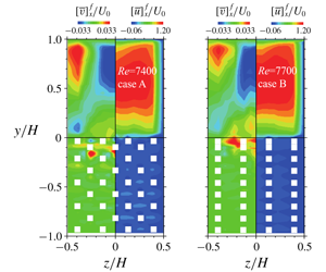
To see the effects of porous structures on the general flow fields, figure 5 compares the time- and streamwise-averaged vertical and streamwise velocity contour maps which are reconstructed using the  $x{-}y$ plane measurement data. Although the structures of cases A and B are very different, irrespective of the Reynolds numbers, the mean velocity distributions in the clear duct region do not look very different from each other. For both the structures, strong downward velocity regions appear at
  $0.4<y/H<0.9$ near the symmetry planes of the clear ducts, while strong upward velocity regions appear towards the top corners. Those distributions are consistent with the secondary currents (figure 3) and the trend of
  $[K_{c}]_{y}$ (figure 4). It is then suggested that the present structural difference does not significantly change the secondary flow patterns in the clear duct regions. As for the flows under the porous interfaces, case B shows stronger upward flows in the central regions than case A due to the structural difference.

Figure 5. Cross-sectional mean velocity contour maps: (a) case A at  $Re=3300$, (b) case A at
  $Re=7400$, (c) case B at
  $Re=3400$ and (d) case B at
  $Re=7700$. The
  $z/H$ location for
  $[\bar{v}]_{x}^{f}$ is reversed for presentation.
3.2 Sectional flow characteristics
To show the examples of the detailed flow distributions inside the porous region, figures 6 and 7 show time-averaged streamwise velocity  $\bar{u}$, Reynolds shear stress
  $-\overline{u^{\prime }v^{\prime }}$ and turbulent intensities (root-mean-square (r.m.s.) velocities)
  $u^{\prime },~v^{\prime }$ in the symmetry planes of
  $z/H=0$ at
  $Re=7400$ and 7700 for cases A and B, respectively. The position of
  $x/D=0$ corresponds to the symmetry plane of the transverse rods shown in figure 2(d). It is clear that, depending on the porous structure, the profiles of the turbulence quantities change significantly. Owing to the structures, the mean velocity shows apparent sinusoidal distribution profiles under the porous surfaces as seen in figures 6(a) and 7(a). However, when we focus on the penetration depth of the Reynolds shear stress shown in figures 6(b) and 7(b), which is assumed to be the length needed for the quantity to reach the asymptotic value under the interface, it is approximately equivalent to the rod height
  $d$. Indeed, the Reynolds shear stress is damped and almost vanishes up to
  $y=-d$. As for the r.m.s. velocities, figure 7(c,d) indicates that the penetration lengths are much longer, suggesting that turbulent fine eddies go deeply into the porous media depending on the porous structure. The budget term analysis for the turbulent flow over a permeable porous layer by Kuwata & Suga (Reference Kuwata and Suga2016b) found that the greater turbulence penetration towards the porous layer was due to the increased redistribution and pressure diffusion processes intensified significantly by the pressure fluctuations. Hence, it is considered that the enhanced turbulent intensities under the porous layer are primarily due to the enhanced pressure fluctuations.

Figure 6. Time-averaged turbulence quantities in the symmetry plane (plane  $z1$ at
  $z/H=0$) in case A at
  $Re=7400$: (a) streamwise velocity, (b) Reynolds shear stress, (c) streamwise r.m.s. velocity and (d) wall-normal r.m.s. velocity. Red broken lines show positions at
  $y=0$ and
  $y=-d$.

Figure 7. Time-averaged turbulence quantities in the symmetry plane (plane  $z1$ at
  $z/H=0$) in case B at
  $Re=7700$: (a) streamwise velocity, (b) Reynolds shear stress, (c) streamwise r.m.s. velocity and (d) wall-normal r.m.s. velocity. Red broken lines show positions at
  $y=0$ and
  $y=-d$.
Figures 8 and 9 compare the sectional distributions of time- and streamwise-averaged quantities for cases A and B at  $Re=$7400 and 7700, respectively. Among the seven planes, planes
  $z1$,
$z1$,  $z4$ and
  $z6$ are plotted. For the streamwise mean velocity, it is clear that the distribution profiles are significantly skewed in the clear duct region of
  $y/H>0$ as seen in figures 8(a) and 9(a). In both cases, the profiles look narrower in the symmetry plane (plane
  $z1$) than in the other planes. This trend is considered to be from the secondary currents and was also seen in Samanta et al. (Reference Samanta, Vinuesa, Lashgari, Schlatter and Brandt2015). Owing to the sidewalls, the secondary flow motions towards the duct corners enhance the flow rate around the duct corners, leading to flatter velocity profiles near the sidewalls. Although the maximum velocities in cases A and B are
  $1.3U_{0}$, the locations of the maximum velocities are at
  $y/H=0.50$ and
  $y/H=0.52$, respectively, which are slightly different from
  $y/H=0.55$ predicted by Samanta et al. (Reference Samanta, Vinuesa, Lashgari, Schlatter and Brandt2015). Since the maximum values of the sinusoidal velocity profiles inside the porous layers are around
  $0.1U_{0}$, the flow rates inside the porous layers are estimated to be less than 5 % of the inlet flow rates. It is clear that the mean velocities in both cases are significantly damped just under the porous surfaces and this trend is consistent with that observed in figures 6(a) and 7(a).

Figure 8. Distributions of streamwise-averaged turbulence quantities of case A at  $Re=7400$: (a) streamwise velocity, (b) Reynolds shear stress, (c) streamwise r.m.s. velocity and (d) wall-normal r.m.s. velocity.

Figure 9. Distributions of streamwise-averaged turbulence quantities of case B at  $Re=7700$: (a) streamwise velocity, (b) Reynolds shear stress, (c) streamwise r.m.s. velocity and (d) wall-normal r.m.s. velocity.
Corresponding to the mean velocities, the streamwise-averaged Reynolds shear stresses of figures 8(b) and 9(b) show asymmetrical profiles in the clear duct region and are steeply damped just under the porous interfaces. As seen in figures 8(c,d) and 9(c,d), the streamwise-averaged r.m.s. velocity fluctuations show significantly different distribution profiles between cases A and B due to the structural difference. It is clear that, although the streamwise r.m.s. profiles drop steeply under the porous surfaces like the mean velocity and the shear stress profiles, the wall-normal r.m.s. profiles do not show such a trend in both cases.
3.3 Streamwise–spanwise plane-averaged flow characteristics
As discussed for figure 3, although the flows are not two-dimensional over the porous surfaces, to see the general characteristics of porous medium flows,  $x$–
$x$– $z$ plane averaging is applied by the trapezoidal rule using the
  $x$–
$x$– $y$ plane measurement data of planes
  $z1$–
$z1$– $z5$ for
  $0\leqslant z/H\leqslant 0.26$. Here, the
  $x$–
$x$– $z$ plane-averaged value is denoted as
  $[\cdot ]_{xz}$. By this procedure, the control area (
 $x$–
$x$– $z$ plane) covers
  $4\times 1$ unit cells of the porous structure along the symmetry plane of the duct. From the time-averaged and
  $x$–
$x$– $z$ plane-averaged (double-averaged) momentum equation (Whitaker Reference Whitaker1996), the total momentum flux across the pores on the porous surface can be written as
 $$\begin{eqnarray}\unicode[STIX]{x1D70F}_{p}=\left(-\unicode[STIX]{x1D70C}[\overline{u^{\prime }v^{\prime }}]_{xz}^{f}-\unicode[STIX]{x1D70C}[\bar{u}]_{xz}^{f}[\bar{v}]_{xz}^{f}-\unicode[STIX]{x1D70C}[\tilde{\bar{u}}\,\tilde{\bar{v}}]_{xz}^{f}+\unicode[STIX]{x1D707}\frac{\unicode[STIX]{x2202}[\bar{u}]_{xz}^{f}}{\unicode[STIX]{x2202}y}\right)_{y=0},\end{eqnarray}$$
 where  $[\tilde{\bar{u}}\,\tilde{\bar{v}}]_{xz}^{f}$ is the dispersion stress in which the dispersion of
  $\bar{u}_{i}$ is defined as
  $\tilde{\bar{u}}_{i}=\bar{u}_{i}-[\bar{u}_{i}]_{xz}^{f}$. Hence, by using the measured quantities, the friction velocity
  $u_{\unicode[STIX]{x1D70F}}^{p}=\sqrt{\unicode[STIX]{x1D70F}_{p}/\unicode[STIX]{x1D70C}}$ on the porous surface can be obtained. Table 2 lists those friction velocities with the other parameters such as the permeability Reynolds numbers.
Table 2. Experimental conditions and measured parameters of the mean velocity fields. Here  $Re$,
$Re$,  $Re_{K_{x}}$,
  $Re_{K_{y}}$ and
  $Re_{K}^{\ast \ast }$ are the Reynolds number based on the inlet velocity
  $U_{0}$, the permeability Reynolds numbers based on
  $\sqrt{\unicode[STIX]{x1D612}_{xx}}$ and
  $\sqrt{\unicode[STIX]{x1D612}_{yy}}$ and the pore-scale Reynolds number defined by (3.5);
  $u_{\unicode[STIX]{x1D70F}}^{p}$ is the friction velocity over the porous wall calculated with the streamwise–spanwise plane-averaged values by (3.2); the boundary layer thickness
  $\unicode[STIX]{x1D6FF}_{w}$ and the slip velocity
  $U_{w}$ are from the plane-averaged mean velocity;
  $\unicode[STIX]{x1D705}$,
  $d_{0}$ and
  $h$ are the von Kármán coefficient, the zero plane displacement and the roughness scale, respectively; and
  $(\cdot )^{p+}$ corresponds to a value normalized by using
  $u_{\unicode[STIX]{x1D70F}}^{p}$.

Figure 10 compares the plane-averaged streamwise mean velocity, Reynolds stress and r.m.s. velocities at  $Re\simeq 7500$. For the velocity profiles in the clear flow region shown in figure 10(a), although there are slight discrepancies between the cases A and B, these two cases show nearly the same profiles. The shown DNS profile of Samanta et al. (Reference Samanta, Vinuesa, Lashgari, Schlatter and Brandt2015) is for the symmetry plane and the Reynolds number is
  $Re_{b}=5000$. Also their porous structure is different from those of the present cases. Even with such differences, the present results are in good accord with the DNS data. The slip velocity
  $U_{w}$ at the porous surface and
  $\unicode[STIX]{x1D6FF}_{w}$, which is the location where the mean velocity has the maximum value, also do not significantly change in the two cases as listed in table 2. They are
  $U_{w}=0.28U_{0}$ and
  $0.30U_{0}$ for cases A and B and
  $\unicode[STIX]{x1D6FF}_{w}=0.52H$ for both cases. From the velocity profiles under the surface, although the sinusoidal profiles of cases A and B are different underneath the surface due to the structural difference, the general trends are similar to each other. When we define the penetration depth as the location to the first local minimum, it is clear that the penetration depths of the mean velocity of both cases are less than
  $y/H=0.06$, which is the height
  $d$ of the square rod constructing the porous media. Corresponding to the mean velocities, the shear stresses of both cases damp quickly until
  $y/H=0.06$. Although some weak sinusoidal profiles are observed in the upper region of the porous layer, they eventually vanish deep inside the porous layer while the mean velocity does not show such a decay. Even though
  $\unicode[STIX]{x1D612}_{yy}$ is 8.3 times larger in case B, the penetration depths of the mean velocity and the Reynolds shear stress do not seem to increase.

Figure 10. Comparison of plane-averaged turbulence quantities at  $Re\simeq 7500$ (at
  $Re=7400$ for case A and
  $Re=7700$ for case B): (a) streamwise velocity, (b) Reynolds shear stress, (c) streamwise and wall-normal r.m.s. velocities and (d) dispersion stresses. The DNS data (Samanta et al. Reference Samanta, Vinuesa, Lashgari, Schlatter and Brandt2015) are at
  $Re_{b}=5000$ in the symmetry plane.
The trend that the flow variables look insensitive to the wall-normal permeability supports our previous conclusion in Suga et al. (Reference Suga, Okazaki, Ho and Kuwata2018), which suggested that, although turbulence generation over porous media was enhanced by the permeable surface, it is rather insensitive to the wall-normal permeability  $\unicode[STIX]{x1D612}_{yy}$ compared with
  $\unicode[STIX]{x1D612}_{xx}$ when
  $R_{y/x}\geqslant 1.0$. We then suggested that flow was reasonably correlated to the permeability Reynolds number
  $Re_{K_{x}}$ based on the streamwise permeability. Indeed, although
  $\unicode[STIX]{x1D612}_{yy}$ of case B is 8.3 times larger than that of case A, the discrepancy between the two cases cannot be considered to reflect such a large difference. Instead of the insensitivity to
  $\unicode[STIX]{x1D612}_{yy}$, Suga et al. (Reference Suga, Okazaki, Ho and Kuwata2018) showed that a 25 % increase of
  $\unicode[STIX]{x1D612}_{xx}$ produced a certain amount of turbulence enhancement. While the fluids penetrating into the porous layer move towards the streamwise or spanwise direction, due to the large turbulent surface shear, most of the penetrating fluids move towards the streamwise direction. Since the penetration depth is not large, it is considered that the moving distances of the penetrating fluids in the streamwise direction are longer than those in the wall-normal direction. Hence, it is considered that among the wall-normal and streamwise permeabilities, the streamwise permeability affects more the turbulence near the porous surface. For the present data including the case at
  $R_{y/x}=0.8$ (case A), as seen in figure 10(b), case A whose
  $\unicode[STIX]{x1D612}_{xx}$ is 19 % larger than that of case B shows 9.8 % larger shear stress near the interface. Also, the profiles of the streamwise r.m.s. velocities shown in figure 10(c) indicate that case A at
  $Re_{K_{x}}=6.37$ is more turbulent than case B at
  $Re_{K_{x}}=5.80$. Hence, the level of surface turbulence follows the order of
  $Re_{K_{x}}$ even including the case of
  $R_{y/x}<1.0$
As for the r.m.s. velocities in figure 10(c), although the plots of the DNS by Samanta et al. (Reference Samanta, Vinuesa, Lashgari, Schlatter and Brandt2015) are for the symmetry plane and applied the averaged friction velocity over the whole porous surface, comparison is made to confirm the turbulence level. The corresponding streamwise permeability Reynolds numbers are  $Re_{K_{x}}=8.90$, 6.37 and 5.80 for the DNS, cases A and B, respectively. Here, for the abscissa
  $\unicode[STIX]{x1D6FF}_{w}$ is the location of the maximum plane-averaged velocity. Although the levels of the present r.m.s. results are in the order of
  $Re_{K_{x}}$, the level of the DNS is somewhat lower than the present experiments even with the higher
  $Re_{K_{x}}$. Indeed, it is seen that, although the levels of the r.m.s. velocities by the DNS are similar to those of the present data, the peak value of the streamwise component and the levels of the r.m.s. velocities in the porous layer are lower than the present experiments. Following Breugem et al. (Reference Breugem, Boersma and Uittenbogaard2006), Samanta et al. (Reference Samanta, Vinuesa, Lashgari, Schlatter and Brandt2015) assumed the permeability and the Forchheimer coefficient as
  $\unicode[STIX]{x1D612}_{\unicode[STIX]{x1D6FC}\unicode[STIX]{x1D6FC}}=d_{p}^{2}\unicode[STIX]{x1D711}^{3}/[180(1-\unicode[STIX]{x1D711})^{2}]$ and
  $\unicode[STIX]{x1D60A}_{\unicode[STIX]{x1D6FC}\unicode[STIX]{x1D6FC}}^{F}=\unicode[STIX]{x1D711}d_{p}/[100(1-\unicode[STIX]{x1D711})]$, where
  $d_{p}$ is the particle size for the loosely packed beds. In the DNS,
  $\unicode[STIX]{x1D711}=0.95$ and
  $d_{p}/H=0.01$ were applied and these values produced the Forchheimer coefficient as
  $\unicode[STIX]{x1D60A}_{\unicode[STIX]{x1D6FC}\unicode[STIX]{x1D6FC}}^{F}/H=1.9\times 10^{-3}$, while in the present cases
  $\unicode[STIX]{x1D60A}_{\unicode[STIX]{x1D6FC}\unicode[STIX]{x1D6FC}}^{F}/H$ is in the range of
  $(1.5{-}6.6)\times 10^{-4}$, which is one order smaller than that of the DNS. Since the effect of a smaller
  $\unicode[STIX]{x1D60A}_{\unicode[STIX]{x1D6FC}\unicode[STIX]{x1D6FC}}^{F}$ is comparable to that of a larger
  $\unicode[STIX]{x1D612}_{\unicode[STIX]{x1D6FC}\unicode[STIX]{x1D6FC}}$, it is considered that, when the larger permeability enhances turbulence, the smaller Forchheimer coefficient also enhances turbulence. Note that in connection with (2.1), the drag force term in the momentum equation can be written as
  $f_{i}=\unicode[STIX]{x1D711}\unicode[STIX]{x1D707}\unicode[STIX]{x1D612}_{ij}^{-1}\langle u_{j}\rangle ^{f}+\unicode[STIX]{x1D711}\unicode[STIX]{x1D707}\unicode[STIX]{x1D612}_{ik}^{-1}\unicode[STIX]{x1D60D}_{kj}\langle u_{j}\rangle ^{f}$. Hence, the Forchheimer tensor works similarly to the inverse of the permeability tensor in the double-averaged equation system. Also the larger Forchheimer coefficient and thus larger form drag caused the steep damping for the r.m.s. velocities inside the porous layer for the DNS.
As far as the profiles inside the porous layer are concerned, both cases A and B show very similar levels of the streamwise and wall-normal r.m.s. velocities while some minor structural effects are seen. Unlike the shear stress profiles, both r.m.s. velocities maintain certain levels and continue decaying inside the porous layer. Obviously the decaying rate is more gentle than those of the mean velocity and the shear stress. It is considered that, although the shear generation is very weak, turbulent vortices penetrate against the upward secondary flow motion and dissipate at a deeper position inside the porous media. Particularly for the wall-normal direction, it is supposed that flow fluctuations are induced by the pressure fluctuations over the surface, which propagate more deeply inside the porous media. These trends confirm the results reported by Breugem et al. (Reference Breugem, Boersma and Uittenbogaard2006) who applied the VANS equation for the porous medium region. Figure 10(d) compares the dispersion stresses  $[\tilde{\bar{u}}_{i}\,\tilde{\bar{u}}_{j}]_{xz}^{f}$. It is obvious that the dispersion stresses are generally very small compared with the turbulent stresses. However, the streamwise component
  $[\tilde{\bar{u}}\,\tilde{\bar{u}}]_{xz}^{f}$ becomes comparable to the turbulent stress only in the region across the porous interface. This trend is consistent with that shown in Kuwata & Suga (Reference Kuwata and Suga2016b).
To see the trend of the r.m.s. velocity in more detail, to smooth the sinusoidal profiles, the square-root values of the volume-averaged  $\overline{u_{i}^{\prime \,2}}$,
 $$\begin{eqnarray}\langle \overline{u_{i}^{\prime \,2}}\rangle ^{f}=\frac{1}{4V_{REV}^{f}}\int _{0}^{D+d}\int _{y}^{y+D_{p_{y}}}\int _{0}^{4(D+d)}\overline{u_{i}^{\prime \,2}}\,\text{d}v^{f},\end{eqnarray}$$
 are plotted in figure 11, where  $V_{REV}^{f}$ is a representative elementary volume (REV) of the porous media defined as the fluid-phase volume of
  $(D+d)\times D_{p_{y}}\times (D+d)$ in the homogeneous structure region. To the REV size in the
  $y$-direction,
  $D_{p_{y}}=4d$ is applied. Although case B has the structural interval of
  $2d$, the structural interval of case A is used for comparison. (Since for both cases the structures are homogeneous at
  $y<-d$, figure 11 shows the values under
  $y/D_{p_{y}}=-0.75$, which is the uppermost location of the REV centre.) For both Reynolds numbers, although the streamwise component is dominant over the surfaces, the wall-normal component surpasses it below the surfaces and becomes dominant until
  $y/D_{p_{y}}\simeq -1.25$ and
  $y/D_{p_{y}}\simeq -1.5$ for cases A and B, respectively. Then, the streamwise component becomes dominant again and maintains the dominance deep inside the porous layer. This trend confirms that the wall-normal fluctuations penetrate more deeply than the streamwise ones while their decaying rate is higher, suggesting that turbulence anisotropy is maintained inside the porous layer. The effects of the wall-normal permeability are not significant enough to change the trend since the difference between the locations where the streamwise component surpasses the wall-normal component is rather small. The present trend of turbulence anisotropy at
  $\unicode[STIX]{x1D711}\simeq 0.8$ and in the range of
  $Re_{K_{x}}=2.49{-}6.37$ is thus consistent with those observed in our previous DNS studies (Kuwata & Suga Reference Kuwata and Suga2016b, Reference Kuwata and Suga2017), which are for
  $\unicode[STIX]{x1D711}=0.7{-}0.84$ at
  $Re_{K}=3.8{-}6.1$.

Figure 11. R.m.s. velocities by the REV averaging: (a) case A and (b) case B, for  $D_{p_{y}}=4d$.

Figure 12. Distributions of the mean velocities and log-law parameters against the pore-scale Reynolds number: (a) streamwise mean velocity distributions in semi-log scale, (b) zero-plane displacement, (c) von Kármán coefficient and (d) roughness scale. The red lines in panel (a) are fitting lines. The data of Breugem et al. (Reference Breugem, Boersma and Uittenbogaard2006), Suga et al. (Reference Suga, Matsumura, Ashitaka, Tominaga and Kaneda2010, Reference Suga, Nakagawa and Kaneda2017), Manes et al. (Reference Manes, Poggi and Ridol2011) and Kuwata & Suga (Reference Kuwata and Suga2016a) are for isotropic porous media, while the data of Kuwata & Suga (Reference Kuwata and Suga2017) and Suga et al. (Reference Suga, Okazaki, Ho and Kuwata2018) are for anisotropic porous media.
To confirm whether the mean velocity profiles near the symmetry plane are similar to those over two-dimensional porous-wall flows, figure 12(a) shows the mean velocities over the porous surfaces in semi-logarithmic charts with fitting lines of the log law:
 $$\begin{eqnarray}[\bar{u}]_{xz}^{p+}=\frac{1}{\unicode[STIX]{x1D705}}\ln \left(\frac{y+d_{0}}{h}\right).\end{eqnarray}$$
 This log-law form is usually applied to flows over porous media and canopies (Best Reference Best1935; Nikora et al. Reference Nikora, Koll, McLean, Dittrich and Aberle2002; Nepf & Ghisalberti Reference Nepf and Ghisalberti2008). Our previous report (Suga et al. Reference Suga, Okazaki, Ho and Kuwata2018) showed that, irrespective of anisotropy of the permeability, the von Kármán coefficient  $\unicode[STIX]{x1D705}$, the zero-plane displacement
  $d_{0}$ and the roughness scale
  $h$ were generally well correlated with the pore-scale Reynolds number
  $Re_{K}^{\ast \ast }$. The pore-scale Reynolds number was defined as
 $$\begin{eqnarray}Re_{K}^{\ast \ast }=\frac{u_{\unicode[STIX]{x1D70F}}^{p}D_{p_{x}}}{3.8\unicode[STIX]{x1D708}},\end{eqnarray}$$
 where  $D_{p_{x}}$ is the streamwise length of the pore. (Note that, since this Reynolds number has a strong correlation with a permeability Reynolds number based on the porosity and the streamwise permeability, Suga et al. (Reference Suga, Okazaki, Ho and Kuwata2018) called it the ‘surrogate’ permeability Reynolds number.) Table 2 lists the values of
  $\unicode[STIX]{x1D705}$,
  $d_{0}^{p+}~(=u_{\unicode[STIX]{x1D70F}}^{p}d_{0}/\unicode[STIX]{x1D708})$ and
  $h^{p+}~(=u_{\unicode[STIX]{x1D70F}}^{p}h/\unicode[STIX]{x1D708})$ that are obtained by the fitting procedure described in Breugem et al. (Reference Breugem, Boersma and Uittenbogaard2006) and Suga et al. (Reference Suga, Matsumura, Ashitaka, Tominaga and Kaneda2010, Reference Suga, Nakagawa and Kaneda2017, Reference Suga, Okazaki, Ho and Kuwata2018). The corresponding figure 12(b–d) shows that the present parameters are well in the clusters of the plots of a wide range of porous-wall flows. This confirms that the turbulent flow over the porous surfaces near the symmetry plane of the square duct maintains the general trend of the mean velocity in the two-dimensional porous-wall turbulence even though the secondary flows are enhanced. Note that for the von Kármán coefficient, the correlation with the pore-scale Reynolds number is not strong compared with the other parameters. Since the zero-plane displacement and the roughness scale are geometrical parameters related to the porous structure, the pore scale is a reasonable parameter for the characteristic length scale. However,
  $\unicode[STIX]{x1D705}y$ corresponds to the mixing length for near-wall turbulence and thus it is considered that the correlation between
  $\unicode[STIX]{x1D705}$ and the pore scale is not very strong.
3.4 Kelvin–Helmholtz instability waves
Samanta et al. (Reference Samanta, Vinuesa, Lashgari, Schlatter and Brandt2015) observed that there were short spanwise rollers in the middle region and their spanwise size was approximately  $0.4H$. Following the discussion by Jiménez et al. (Reference Jiménez, Uhlmann, Pinelli and Kawahara2001), those spanwise rollers are considered to be induced by the KH instability since the mean velocity has an inflection point under the porous surface as seen in figure 10. Although Samanta et al. (Reference Samanta, Vinuesa, Lashgari, Schlatter and Brandt2015) did not analyse the characteristics of those rollers, we try to detect and analyse the wave motions over porous media. Figure 13 shows the one-dimensional spectrum of streamwise velocity fluctuations
  $E_{11,x}$ at
  $y/H=0.1$,
  $0.0$ and
  $-0.02$ in the symmetry planes. Those locations correspond to over, at and under the surface, respectively. For
  $Re\simeq 3500$,
  $y/H=0.1$ and
  $-0.02$ correspond to
  $y^{p+}\simeq 30$ and
  $-6$, respectively, while for
  $Re\simeq 7500$, they correspond to
  $y^{p+}\simeq 75$ and
  $-15$, respectively. Both cases A and B at the surfaces (
 $y/H=0$) show clear peaks. At
  $Re\simeq 3500$ shown in figure 13(a,b), the peaks of
  $y/H=0.0$ are located at
  $f=0.25~\text{Hz}$, which corresponds to the wavelength of
  $\unicode[STIX]{x1D706}_{w}=U_{w}/f=1.4H$ due to the slippage velocity of
  $U_{w}=0.28U_{0}$ as listed in table 2. At
  $Re\simeq 7500$ of case A, the peak of
  $y/H=0.0$ is located at
  $f=0.5~\text{Hz}$, which corresponds to the wavelength of
  $\unicode[STIX]{x1D706}_{w}=1.8H$, while for case B, it is located at
  $f=0.6~\text{Hz}$, which corresponds to the wavelength of
  $\unicode[STIX]{x1D706}_{w}=1.6H$ since
  $U_{w}$ increases to
  $0.3U_{0}$. Accordingly, clear effects of the wall-normal permeability on the wavelengths are not observed also. Although the locations of the peaks of
  $y/H=-0.02$ shift slightly from those of
  $y/H=0.0$, the corresponding frequencies are very similar to those of
  $y/H=0.0$. This is because the energy of the waves generated at the surfaces propagates to both over- and under-surface regions.

Figure 13. One-dimensional streamwise spectrum of  $u^{\prime }$ in the symmetry plane: (a) case A at
  $Re=3300$, (b) case B at
  $Re=3400$, (c) case A at
  $Re=7400$ and (d) case B at
  $Re=7700$. Black broken vertical lines correspond to the frequencies of peak locations at the surface:
  $y/H=0.0$.
In the fully developed mixing layers, the wavelength of the KH-type coherent eddies normalized by the vorticity thickness,  $C_{\unicode[STIX]{x1D706}}=\unicode[STIX]{x1D706}_{x}/\unicode[STIX]{x1D6FF}_{\unicode[STIX]{x1D6FA}}$, is known to be
  $3.5\leqslant C_{\unicode[STIX]{x1D706}}\leqslant 5$ (Dimotakis & Brown Reference Dimotakis and Brown1976; Rogers & Moser Reference Rogers and Moser1994). For flows over porous walls, the DNS by Breugem et al. (Reference Breugem, Boersma and Uittenbogaard2006) and Kuwata & Suga (Reference Kuwata and Suga2017) and the experiments by Suga et al. (Reference Suga, Okazaki, Ho and Kuwata2018) indicated
  $3.4\leqslant C_{\unicode[STIX]{x1D706}}\leqslant 5.5$ when the boundary layer thickness
  $\unicode[STIX]{x1D6FF}_{w}$ is considered to be equivalent to the vorticity thickness
  $\unicode[STIX]{x1D6FF}_{\unicode[STIX]{x1D6FA}}$. The wavelength
  $\unicode[STIX]{x1D706}_{w}$ of cases A and B at
  $Re\simeq 3500$ produces
  $C_{\unicode[STIX]{x1D706}}=\unicode[STIX]{x1D706}_{w}/\unicode[STIX]{x1D6FF}_{w}=3.0$ and 2.9, respectively. At
  $Re\simeq 7500$, for cases A and B they are
  $C_{\unicode[STIX]{x1D706}}=3.5$ and 3.1, respectively. Although these values are close to the range of the reported values for KH waves, they are somewhat smaller than the reported values of turbulence over porous media. Although there are many unknown things regarding the interaction between the KH instability and the sidewall turbulent boundary layers, we believe that such interaction influences the instability, resulting in shorter wavelengths than those in two-dimensional boundary layer type of flows. This sidewall confinement effect is stronger at lower Reynolds numbers since the sidewall boundary layer is thicker at lower Reynolds number as seen in figure 3.
4 Conclusions
PIV measurements have been carried out for fully developed turbulent square duct flows over two transparent anisotropic porous media whose porosity is  $\unicode[STIX]{x1D711}\simeq 0.8$ and ratios of the wall-normal to streamwise permeabilities are
  $R_{y/x}=0.8$ and 7.8 at
  $Re\simeq 3500$ and 7500. The corresponding streamwise permeability Reynolds numbers are
  $Re_{K_{x}}=2.49$–6.37, while the wall-normal permeability Reynolds numbers are
  $Re_{K_{y}}=2.37$–16.20. It is observed that, irrespective of the porous structure, the well-known four sets of counter-rotating secondary flow patterns in the square cross-section changes to a flow pattern having one large recirculation near each solid corner accompanied by a weak counter-rotation towards the porous corner. Although the porous structure is very different, this flow pattern is the same as that shown in the DNS of Samanta et al. (Reference Samanta, Vinuesa, Lashgari, Schlatter and Brandt2015). The maximum magnitude of the secondary currents is approximately 6 % of the inlet bulk velocity, which is a little smaller than that of the DNS.
It is confirmed that, although turbulence is enhanced by the permeability, turbulence over and under the porous surface is rather insensitive to the wall-normal permeability compared with the streamwise component. Accordingly,  $Re_{K_{x}}$ is a better parameter that correlates to the porous-wall turbulence at least for
  $R_{y/x}\geqslant 0.8$. It is also confirmed that the r.m.s. velocities penetrate more deeply than the mean velocity and the wall-normal fluctuations need a longer distance to be damped in the porous media than the streamwise component. This suggests that, although there is no shear generation, turbulent vortices penetrate against the upward secondary flow motion and dissipate at deeper locations inside porous media. It is considered that velocity fluctuations are drawn into the porous media by the pressure fluctuations over the surface, which propagate more deeply inside the porous media. Accordingly, a little under the surface the wall-normal r.m.s. velocity becomes larger than the streamwise component while the streamwise r.m.s. velocity becomes dominant again deep inside the porous layer. However, interestingly, the effect of the wall-normal permeability is also insignificant even for the penetration.
For the streamwise–spanwise plane-averaged mean velocity near the symmetry plane, the correlations between the pore-scale Reynolds number and the log-law parameters such as the zero plane displacement, the von Kármán coefficient and the roughness scale are confirmed to be similar to those seen in a wide range of porous-wall turbulence. The wavelengths of the spanwise rollers near the symmetry planes generated by a KH-type instability are detected at the porous surfaces. While significant effects of the porous structure on the wavelengths are not observed, it is found that the wavelength tends to be shorter than those of porous-wall channels possibly by the sidewall effects while such a trend becomes weaker at higher Reynolds numbers. Overall, even with the enhanced secondary flows, near-porous-wall turbulence characteristics in the middle of the porous square duct are very similar to those of porous-wall turbulent boundary layers while the sidewall effects become apparent at low Reynolds numbers.
Acknowledgements
The authors express their gratitude to their colleagues, Messrs T. Iida, A. Taneo, R. Okabe, T. Matsuo and K. Igarashi and Dr Masayuki Kaneda, who assisted in performing the experiments. A part of this study was financially supported by the research grant (no. 24360073) of the JSPS.
Declaration of interests
The authors report no conflict of interest.
Appendix. Confirmation of the flow development
The position of the measuring section in this study is located at  $X=2.7~\text{m}$ (
 $X/H=54$) from the duct inlet. Here,
  $X$ is the streamwise distance from the duct inlet. In the preliminary experiments, we measured flow quantities in the centre (symmetry) plane of the clear fluid region at several locations. Figure 14 compares turbulence quantities at
  $X/H=38$, 50 and 54 for
  $Re\simeq 8000$. It is seen that, although the mean velocity profiles at the three locations are almost the same, the Reynolds shear stress and the r.m.s. velocities at
  $X/H=38$ do not converge at the same levels of those at
  $X/H\geqslant 50$. It thus indicates that the flow is not fully developed yet at
  $X/H=38$. Since there is no meaningful difference in the turbulence quantities at
  $X/H=50$ and 54, it can be said that the flow is fully developed at least by
  $x/D=50$. Therefore, it is confirmed that the presently measured flows are fully developed at the present measuring position at
  $X/H=54$ for the cases at
  $Re\leqslant 8000$.

Figure 14. Comparison of the centre-plane turbulence quantities of case B at  $Re\simeq 8000$: (a) mean velocity, (b) Reynolds shear stress, (c) streamwise r.m.s. velocity and (d) wall-normal r.m.s. velocity.


