


1. Introduction
Fick's diffusion (Gardiner Reference Gardiner2009) implies that the directed displacements of an overdamped Brownian particle, say, in the  $x$ direction,
  ${\rm \Delta} x(t)=x(t)-x(0)$, grow with time following the Einstein law,
  $\langle {\rm \Delta} x^{2}(t) \rangle = 2Dt$, and with Gaussian statistics. Accordingly, the probability density function (p.d.f.) of the rescaled observable,
  ${\rm \Delta} x/\sqrt {t}$, would be a stationary Gaussian distribution with half-variance
  $D$.
$D$.
Recent observations (Wang et al. Reference Wang, Anthony, Bae and Granick2009; Wang et al. Reference Wang, Kuo, Bae and Granick2012; Bhattacharya et al. Reference Bhattacharya, Sharma, Saurabh, De, Sain, Nandi and Chowdhury2013; Kim, Kim & Sung Reference Kim, Kim and Sung2013; Guan, Wang & Granick Reference Guan, Wang and Granick2014; Kwon, Sung & Yethiraj Reference Kwon, Sung and Yethiraj2014) of Brownian motion in fluctuating crowded environments led to questions regarding the generality of such a notion. Indeed, there are no a priori reasons why the diffusion of a physical Brownian tracer should be of Fickian type. For instance, in real biophysical systems displacement p.d.f.s often exhibit prominent exponential tails over wide intervals of the observation time,  $t$, well after the condition of normal diffusion has set in. Such a transient effect, termed here non-Gaussian normal diffusion (NGND), is expected to disappear for asymptotically large observation times (possibly inaccessible to real experiments Wang et al. Reference Wang, Anthony, Bae and Granick2009), as stipulated by the central limit theorem. In that limit, the
  ${\rm \Delta} x$ distributions turn eventually Gaussian, with half-variance equal to
  $\langle {\rm \Delta} x^{2}(t) \rangle$. Persistent diffusive transients of this type have been detected in diverse experimental set-ups (Weeks et al. Reference Weeks, Crocker, Levitt, Schofield and Weitz2000; Eaves & Reichman Reference Eaves and Reichman2009; Leptos et al. Reference Leptos, Guasto, Gollub, Pesci and Goldstein2009; Wang et al. Reference Wang, Anthony, Bae and Granick2009; Wang et al. Reference Wang, Kuo, Bae and Granick2012; Bhattacharya et al. Reference Bhattacharya, Sharma, Saurabh, De, Sain, Nandi and Chowdhury2013), and further confirmed by extensive numerical simulations (Kegel & van Blaaderen Reference Kegel and van Blaaderen2000; Chaudhuri, Berthier & Kob Reference Chaudhuri, Berthier and Kob2007; Guan et al. Reference Guan, Wang and Granick2014; Kwon et al. Reference Kwon, Sung and Yethiraj2014; Ghosh et al. Reference Ghosh, Cherstvy, Grebenkov and Metzler2016; He et al. Reference He, Song, Su, Geng, Ackerson, Peng and Tong2016).
The current interpretation of this phenomenon postulates that diffusion occurs in a fluctuating environment with finite relaxation time,  $\tau$ (Wang et al. Reference Wang, Anthony, Bae and Granick2009). For observation times comparable with
  $\tau$, the tracer displacements are likely to obey a non-Gaussian statistics. The rescaled p.d.f.s,
  $p({\rm \Delta} x/\sqrt {t})$, are typically Gaussian for either much shorter or much larger
  $t$ values, although with different half-variance: the free diffusion constant,
  $D_0$, for
  $t \to 0$ (no crowding effect) and the asymptotic diffusion constant,
  $D$, defined above, for
  $t \to \infty$ (central limit theorem). There is no fundamental reason why non-Gaussian transients should necessarily lead to the emergence of slowly decaying distribution tails (leptokurtic transients), as reported in the current literature; on the contrary, one cannot rule out the possibility that, under certain conditions, their tails decay faster than a Gaussian tail (platykurtic transients). Moreover, the NGND phenomenon can also occur in low-dimensional models, though restricted to relatively narrow
  $t$ domains (Li et al. Reference Li, Marchesoni, Debnath and Ghosh2019).
We investigate here, both numerically and analytically, the Brownian diffusion of an overdamped particle suspended in a periodic array of planar convection rolls, subjected to thermal fluctuations of strength  $D_0$. This is an archetypal model with well-established applications to physical systems of the most diverse length scales (Chandrasekhar Reference Chandrasekhar1967; Tabeling Reference Tabeling2002; Kirby Reference Kirby2010). At high Péclet numbers, i.e. when the effects of thermal fluctuations are negligible with respect to advection, the particle undergoes normal diffusion with asymptotic diffusion constant,
  $D$, which depends on both
  $D_0$ and the flow parameters (Rosenbluth et al. Reference Rosenbluth, Berk, Doxas and Horton1987). The ensuing NGND is characterized by a single transient time,
  $\tau$, but, in contrast with other elementary models (Li et al. Reference Li, Marchesoni, Debnath and Ghosh2019),
  $\tau$ is controlled by two competing microscopic mechanisms depending on
  $D_0$. At low thermal noise, the transient dynamics of the particle is governed by its isotropic random jumps from roll to roll, a stochastic process quite insensitive to the details of the particle's trajectory inside each individual roll. On the contrary, upon raising the thermal noise (but still at high Péclet numbers), roll jumping grows faster compared with the circulation inside the rolls. The diffusion transient dynamics is then dominated by the advective drag. Accordingly, one defines two distinct time scales, namely, the mean time for the particle to first exit the convection rolls and its average revolution period inside a single roll. The peculiarity of this system is that, upon increasing the noise strength, the NGND transients can change from lepto- to platykurtic, depending on which of such two time scales is larger and, thus, plays the role of effective transient time,
  $\tau$.
The problem we address is also of practical interest in view of its applications to microfluidics (Kirby Reference Kirby2010), chemical engineering and combustion (Moffatt et al. Reference Moffatt, Zaslavsky, Comte and Tabor1992) and the modelling of large-scale geodynamic processes (Tabeling Reference Tabeling2002). Indeed, the experimental or numerical determination of the asymptotic mean-square displacement of a tracer in a convective flow can take exceedingly long times to allow it to jump repeatedly from convection roll to convection roll. On the contrary, in a number of physical situations the observer only needs to determine how long a trapped tracer will sojourn inside a single roll before crossing its flow boundary layer into a neighbouring one. This quantity is more easily accessible to direct observation and, as shown at the end of this paper, influences the non-Gaussian properties of the tracer's transient displacement distributions. Stated otherwise, from displacement distributions obtained for finite observation times, we cannot extract the asymptotic diffusion constant,  $D$, with a high degree of confidence, if the non-Gaussian transients of the underlying diffusive process are unpredictably long.
The present paper is organized as follows. In § 2 we introduce the Langevin equations that describe Brownian diffusion in a two-dimensional laminar flow patterned as a periodic array of counter-rotating convection rolls. Following Rosenbluth et al. (Reference Rosenbluth, Berk, Doxas and Horton1987), we distinguish between the regime of high Péclet numbers, relevant to this work, where diffusion is governed by advection, and the best known regime of thermal diffusion, dominated by equilibrium fluctuations. In § 3 we investigate the two time scales controlling Brownian diffusion in a periodic array of convection rolls, namely, the average period of fluid circulation inside a roll (§ 3.1) and the particle's mean first-exit time out of a single roll (§ 3.2). In § 4 we present detailed numerical evidence of the NGND phenomenon. Lepto- and platykurtic transients are qualitatively explained by time coarse graining the microscopic particle dynamics and quantified by fitting our numerical displacement distributions by means of a phenomenological one-parameter function. Finally, in § 5 we draw some concluding remarks.
2. Model: periodic array of counter-rotating convection rolls
For this purpose we investigated the diffusion of an overdamped particle of unit mass, coordinates  $x$ and
  $y$, suspended in a two-dimensional (2-D) stationary laminar flow with periodic centre-symmetric streamfunction
 \begin{equation} \psi(x,y)= ({U_0L}/{2{\rm \pi}})\sin({2{\rm \pi} x}/{L})\sin({2{\rm \pi} y}/{L}), \end{equation}
where  $U_0$ is the maximum advection speed and
  $L$ the size of the flow unit cell. Following the earlier literature (Chandrasekhar Reference Chandrasekhar1967; Childress Reference Childress1979; Rosenbluth et al. Reference Rosenbluth, Berk, Doxas and Horton1987; Soward Reference Soward1987), we assumed that the particle is perfectly spherical and so small that it can be taken as point like. Accordingly, away from confining boundaries or other particles (low particle density approximation) hydrodynamic interactions and flow torques were ignored. Its dynamics can thus be formulated by means of two translational Langevin equations,
 \begin{equation} \dot {x}= u_x + \xi_x(t),\quad \dot {y}= u_y + \xi_y(t), \end{equation}
where the vector  ${ \boldsymbol u}=(u_x, u_y) =(\partial _y, -\partial _x)\psi$ is the advection velocity. As illustrated in figure 1(a),
  $\psi (x,y)$ defines four counter-rotating flow subcells, also termed convection rolls. The translational noises,
  $\xi _i(t)$ with
  $i=x,y$ are stationary, independent, delta-correlated Gaussian noises,
  $\langle \xi _i(t)\xi _j(0)\rangle = 2 D_0 \delta _{ij}\delta (t)$, where
  $\delta_{ij}$ and
  $\delta(t)$ are respectively the Kronecker and Dirac delta. They can be regarded as modelling equilibrium thermal fluctuations in a homogeneous, isotropic medium, with
  $D_0$ proportional to its temperature. In the present notation,
  $D_0$ is the free particle diffusion constant in the absence of advection. In our simulations, we used the flow parameters,
  $U_0$ and
  $L$ to set convenient length and time units, respectively,
  $L$ and
  $L/2{\rm \pi} U_0$. Therefore, the only tuneable parameter left in our analysis is the noise strength,
  $D_0$. As we are interested in the diffusion properties under stationary conditions, we assumed a uniform random distribution of the particle's initial coordinates,
  $x_0$ and
  $y_0$. Indeed, due to the incompressibility of the advection vector,
  $(u_x,u_y)$, in the presence of thermal noise, a particle's trajectory is known to eventually fill up the
  $x,y$ plane uniformly.

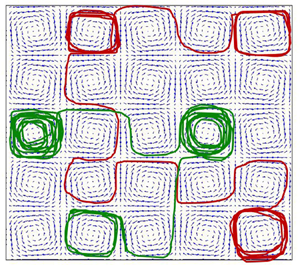
Figure 1. Diffusion of a Brownian particle in a two-dimensional periodic pattern of stationary convection rolls. (a) Unit flow cell, (2.1), consisting of four counter-rotating subcells. (b) Trajectory sample of length  $t=100$, for
  $D_0=0.001$. Flow parameters are:
  $U_0=1$ and
  $L=2{\rm \pi}$.
The amplitude of  $\psi (x,y)$ in (2.1) provides a natural diffusion scale of the convective flow,
  $D_L=U_0 L/2{\rm \pi}$; accordingly the Péclet number of the advected Brownian particle is defined here as
  $\textrm {Pe}\equiv D_L/D_0>1$.
The stochastic differential equations (2.2a,b) were numerically integrated by means of a standard Mil'shtein scheme (Kloeden & Platen Reference Kloeden and Platen1992). Particular caution was exerted when computing the values of the asymptotic diffusion constant
 \begin{equation} D=\lim_{t\to \infty} \langle {\rm \Delta} x^{2}(t)\rangle /2t. \end{equation}
Indeed, upon lowering the noise strength,  $D_0$, the roll jumping of the advected particle is suppressed; accordingly, the transient time,
  $\tau$, grows exceedingly long. Even if during such transients instances of anomalous diffusion may become detectable (Young, Pumir & Pomeau Reference Young, Pumir and Pomeau1989), in this paper we focus on the normal diffusion limit in (2.3).
Particle transport in such a flow pattern has been studied under diverse physical conditions and a rich phenomenology has emerged (Shraiman Reference Shraiman1987; Solomon & Gollub Reference Solomon and Gollub1988; Young et al. Reference Young, Pumir and Pomeau1989; Solomon & Mezić Reference Solomon and Mezić2003; Torney & Neufeld Reference Torney and Neufeld2007; Young & Shelley Reference Young and Shelley2007; Manikantan & Saintillan Reference Manikantan and Saintillan2013; Sarracino et al. Reference Sarracino, Cecconi, Puglisi and Vulpiani2016; Li et al. Reference Li, Li, Marchesoni, Debnath and Ghosh2020). For instance, in the presence of external periodic perturbations the deterministic dynamics of a noiseless particle exhibits remarkable chaotic properties (Solomon & Gollub Reference Solomon and Gollub1988; Solomon & Mezić Reference Solomon and Mezić2003). Especially relevant to the present work are the results for the diffusivity of a point-like Brownian tracer first reported in Rosenbluth et al. (Reference Rosenbluth, Berk, Doxas and Horton1987). The problem of how a flow field of streamfunction  $\psi (x,y)$ affects the diffusion of a self-propelled particle has been investigated in Torney & Neufeld (Reference Torney and Neufeld2007) and Li et al. (Reference Li, Li, Marchesoni, Debnath and Ghosh2020).
The Langevin equations (2.2a,b) model particle diffusion under the simultaneous action of translational fluctuations and advective drag. An important property of this system is illustrated in figure 2, where we have plotted the asymptotic diffusion constant,  $D$, as a function on the noise intensity (and free diffusion constant),
  $D_0$. The mean-square displacement approaches asymptotically the Einstein law for any choice of
  $D_0$. However, on increasing
  $D_0$, the asymptotic diffusion constant,
  $D$, changes from
 \begin{equation} D=\kappa\sqrt{D_L D_0}, \end{equation}
for  $D_0< D_L$ (dispersive transport), to
 \begin{equation} D=D_0, \end{equation}
for  $D_0>D_L$ (diffusive transport). The constant
  $\kappa$ in (2.4) depends on the geometry of the flow cells (Rosenbluth et al. Reference Rosenbluth, Berk, Doxas and Horton1987; Young et al. Reference Young, Pumir and Pomeau1989). For the 2-D array of square counter-rotating convection rolls of (2.1),
  $\kappa \simeq 1.06$ (Rosenbluth et al. Reference Rosenbluth, Berk, Doxas and Horton1987), in close agreement with the numerical results displayed in figure 2.

Figure 2. Diffusion in the periodic convective flow pattern of (2.1):  $D$ vs.
  $D_0$, both rescaled by
  $D_L=U_0L/2{\rm \pi}$. The analytical predictions for low-noise, (2.4), and high-noise, (2.5), strengths are represented by solid lines. Within our numerical accuracy, the fitted value of
  $\kappa$ is consistent with the predicted value,
  $1.06$ (Rosenbluth et al. Reference Rosenbluth, Berk, Doxas and Horton1987). The streamfunction parameters are
  $U_0=1$ and
  $L=2{\rm \pi}$, so that
  $D_L=1$.
The cross-over between the two diffusion regimes occurs at  $D_0\simeq D_L$ and appears to be quite sharp (Li et al. Reference Li, Li, Marchesoni, Debnath and Ghosh2020). This property was explained (Rosenbluth et al. Reference Rosenbluth, Berk, Doxas and Horton1987; Soward Reference Soward1987; Young et al. Reference Young, Pumir and Pomeau1989) by noticing that, for
  $D < D_L$, spatial diffusion occurs within the boundary flow layers delimiting the four subcells of the streamfunction,
  $\psi (x,y)$, as illustrated in figure 3(a). Stated otherwise, the diffusion process is governed by the advection velocity field. Vice versa, for
  $D_0>D_L$, the effects of advection on the particle's diffusion become negligible. In view of the above, NGND is more likely to happen in the regime of advective transport; therefore, we focus our discussion on the high Péclet number domain.

Figure 3. Exit mechanism from a flow cell. (a) Spatial distribution of a particle injected at the centre of the top-left roll,  $(-L/2,L/2)$, in a box with absorbing boundaries
  $x,y=\pm L/2$, and subjected to noise of strength
  $D_0=0.01$; the side bar is the relevant amplitude colour code on a natural logarithmic scale. Distribution computed over 10
 $^{7}$ trajectories with integration time step of 10
 $^{-5}$. (b) Distributions,
  $P(T)$, of the particle's exit times,
  $T$, for different
  $D_0$ (filled symbols, see legend). For comparison (see text), the
  $P(T)$ curves for
  $D_0=3\times 10^{-3}$ and
  $10^{-2}$ have been ‘stretched’ by rescaling
  $T\to 4T$ (empty symbols). The streamfunction parameters are
  $U_0=1$ and
  $L=2{\rm \pi}$. Power laws are drawn to fit the
  $T\to 0$ branches of the low- and high-noise distributions. Note that in dimensionless units, simulation results for
  $U_0=0$ correspond to taking the limit
  $D_0\to \infty$.
3. Relevant time scales
The particle dynamics of (2.1) and (2.2a,b) results from the superposition of an advective drag with velocity  ${ \boldsymbol u}$ and a free Brownian motion driven by thermal fluctuations. Advection pulls the particle along closed orbits inside each
  $\psi (x,y)$ subcell, either clock- or anticlockwise, whereas thermal noise pushes the particle eventually over the subcell boundaries. Both mechanisms play a key role in our discussion of the ensuing NGND phenomenon. Therefore, in the next subsections we briefly derive their characteristic time scales.
3.1. Advection period
To analyse roll circulation we consider the ‘positive’  $\psi (x,y)$ subcell centred at
  $(L/4,L/4)$, see figure 1(a), where the particle circulates anticlockwise. In the noiseless regime with
  $D_0=0$, a simple time derivation of both sides of (2.1) yields two decoupled equations,
 \begin{equation} \ddot x'=\varOmega_L^{2} \sin x',\quad \ddot y'=\varOmega_L^{2} \sin y', \end{equation}
for the rescaled coordinates  $x'=2(2{\rm \pi} x/L)$ and
  $y'=2(2{\rm \pi} y/L)$. Here, the angular frequency
  $\varOmega _L=2{\rm \pi} U_0/L$ coincides with the maximum vorticity,
  ${ \boldsymbol \nabla } \wedge { \boldsymbol u}=-\nabla ^{2}\psi$, at the centre of the convection roll. Both (3.1a,b) describe a mathematical pendulum centred at
  $({\rm \pi} ,{\rm \pi} )$ – the subcell centre. This implies that, due to the
  $x\leftrightarrow y$ symmetry of
  $\psi (x,y)$, the period of the particle's orbits,
  $T_L$, depends on their maximum amplitude,
  $a_0$, along either the
  $x$ or
  $y$ direction (orbits are not circular!) with
  $a_0< {\rm \pi}$. The function
  $T_L(a_0)$ can be expressed analytically as the period of either physical pendulum in (3.1a,b),
 \begin{equation} T_L(a_0)=\frac{2T_0}{\rm \pi}~K(k), \end{equation}
where  $T_0=2{\rm \pi} /\varOmega _L$,
  $k=\sin (a_0/2)$ and
  $K(k)$ is a complete elliptic integral of first kind (Cromer Reference Cromer1995). The logarithmic divergence of
  $T_L$ for
  $a_0\to {\rm \pi}$ is best approximated by (Cromer Reference Cromer1995)
  $T_L (a_0)=(2T_0/{\rm \pi} )\ln [4/\cos (a_0/2)]$. This implies that, in the absence of thermal fluctuations, the particle gets trapped in a convection roll. Despite its simple derivation, our result for
  $T_L$ is consistent with earlier estimates (Weiss Reference Weiss1966).
Under stationary conditions, the particle's spatial distribution is uniform. Accordingly, the density function of  $a_0$ is well approximated by
  $2a_0/{\rm \pi}$. In the limit of very high Péclet numbers,
  $\textrm {Pe}\gg 1$, a useful estimate of the advection period can be obtained by averaging
  $T_L(a_0)$ with respect to
  $a_0$, namely (Gradshteyn & Ryzhik Reference Gradshteyn and Ryzhik2007),
 \begin{equation} T_L=\langle T_L(a_0)\rangle= 2.786 T_0. \end{equation}
In view of our derivation, it is clear that this result holds only in the limit  $D_0\to 0+$ (Yin et al. Reference Yin, Li, Marchesoni, Debnath and Ghosh2021). We reiterate that, for
  $D_0\equiv 0$, diffusion is completely suppressed.
3.2. Mean first-exit time
To estimate the mean first-exit time (MFET) of the particle out of the flow unit cell, we calculate first the MFET of a free Brownian particle out of a square box of size  $L$. In the absence of advection,
  $U_0=0$, this can be done analytically by standard stochastic methods – see (5.4.37) of Gardiner (Reference Gardiner2009), where a typo had to be corrected. For a particle starting at
  $(x_0,y_0)$ inside a box of vertices
  $x=\pm L/2$ and
  $y=\pm L/2$, the MFET is
 \begin{align} T (x_0,y_0) &= \frac{1}{D_0} \left (\frac{L}{2{\rm \pi}} \right )^{2}\left ( \frac{8}{\rm \pi}\right )^{2} \sum_{m,n}^{(\rm odd)}\frac{1}{mn}\frac{1}{m^{2}+n^{2}} \nonumber\\ &\quad \times \sin\left [{{\rm \pi} n}\left (\frac {x_0}{L}-\frac{1}{2} \right ) \right] \sin\left [{{\rm \pi} m}\left (\frac{y_0}{L}-\frac{1}{2} \right ) \right], \end{align}
where the summation is restricted to the odd values of  $m$ and
  $n$. Under stationary conditions, the spatial distribution of the particle is uniform. Therefore, we average
  $T(x_0,y_0)$ with respect the particle's initial position,
  $(x_0,y_0)$, to obtain the spatially averaged MFET,
 \begin{equation} \langle T (x_0,y_0)\rangle =\frac{L^{2}}{D_0} \left ( \frac{2}{\rm \pi}\right )^{6}\sum_{m,n}^{(\rm odd)} \frac{1}{m^{2}}\frac{1}{n^{2}}\frac{1}{m^{2}+n^{2}}. \end{equation}
 We next investigate the MFET for a Brownian tracer to escape from a unit cell of the streamfunction  $\psi (x,y)$. Let
  $T_D$ denote the spatial average of such a MFET, with spatial average taken over a unit flow cell. In the purely diffusive regime of (2.5),
  $D_0\gg D_L$, the effect of advection is negligible; hence,
  $T_D=\langle T (x_0,y_0)\rangle$. In the opposite limit of advective diffusion,
  $D_0\ll D_L$, as apparent from figures 1(b) and 3(a), the exit process consists of a slow activation mechanism, where the particle thermally diffuses from the centre of a subcell toward its boundaries, followed by a relatively faster propagation driven by the laminar flow, which runs parallel to the separatrices delimiting the adjacent counter-rotating subcells. This statement is based on the fact that, for
  $D_0\to 0$,
  $T_D$ diverges like
  $1/D_0$, (3.5), whereas
  $T_L$ diverges like
  $T_L \sim (T_0/{\rm \pi} )\ln (D_L/D_0)$. This last result follows from the logarithmic divergence of
  $T_L$ in the limit
  $a_0\to {\rm \pi}$, which we derived in § 3.1. There,
  $|{\rm \pi} -a_0|$ was a measure of the particle's distance from the roll separatrices, which, in dimensional units, reads
  $\delta = (L/2{\rm \pi} )|1-a_0/{\rm \pi} |$. In the presence of noise, the particle mean-square displacement over the advection period
  $T_0$ gives a simple estimate of
  $\delta$,
  $\delta ^{2}=2D_0T_0$, which one may interpret as the effective width of the rolls’ boundary flow layers (Rosenbluth et al. Reference Rosenbluth, Berk, Doxas and Horton1987).
Consider now a particle trapped in a convection roll, say, in the top-left  $\psi (x,y)$ subcell of figure 3(a). To leave the simulation box, it first slowly free diffuses inside the trapping subcell; it is only upon reaching the subcell boundary layer, that it gets swept away by the advection flow along the square net formed by the roll separatrices, as illustrated in figure 1(b). In the limit
  $D_0/D_L \to 0$, the advection period
  $T_L$ grows negligible with respect to any exit diffusion time, so that the particle's MFET out of a unit
  $\psi (x,y)$ cell,
  $T_D$, tends to coincide with the particle's free diffusion time out of a single subcell. The latter time can be calculated by simply replacing
  $L$ with
  $L/2$ in (3.5). In conclusion, we expect that for
  $\textrm {Pe}\gg 1$,
  $T_D=(1/4)\langle T (x_0,y_0)\rangle$. Our analytical estimates of
  $T_D$ are in good agreement with the numerical data displayed in figure 4, which well illustrates the transition between the low- and high-noise regimes of
  $T_D$.

Figure 4. Diffusion mechanisms in the periodic flow pattern of streamfunction  $\psi (x,y)$, (2.1): (a)
  $T_D$, vs. thermal noise,
  $D_0$. The asymptotic solid lines on the left and right are respectively
  $\langle T(x_0,y_0)\rangle$ and
  $(1/4)\langle T (x_0,y_0)\rangle$, (3.5); the horizontal dashed line represents the advection period
  $T_0$. Three
  $D_0$ intervals with distinct ranges of the fitting parameter
  $\beta$ of (4.1) are delimited by the vertical lines
  $D_0=D^{*}$ and
  $D_0=D_L$ and shaded in different colours; no NGND was detected for
  $D_0>D_L$. The value of
  $D^{*}$ was obtained by numerically solving the equation
  $T_D=T_0$ (see text). (b) Value of
  $\langle {\rm \Delta} x^{2}(t) \rangle$ vs.
  $t$ for different
  $D_0$. Vertical arrows denote the onset time of normal diffusion,
  $t=T_D$. Convection flow parameters are
  $U_0=1$ and
  $L=2{\rm \pi}$.
Both limiting estimates for  $T_D$ ignore advection and, therefore, differ by just a geometric factor 4, that is the ratio of the cell-to-subcell areas. The predominance of this geometric factor is apparent also in figure 3(b), where first-exit time distributions,
  $P(T)$, have been plotted for low- and high-noise strengths. To numerically determine
  $P(T)$, first we computed the first-exit times,
  $T$, for a fixed starting point
  $(x_0,y_0)$; then we averaged the relevant p.d.f.s by taking a uniform distribution of
  $(x_0,y_0)$ over a full unit flow cell. For the sake of a comparison, we also plotted the distributions for the two lowest values of
  $D_0$ on the dilated scale
  $T \to 4T$. The high-noise distributions,
  $P(T)$, and such ‘stretched’ low-noise distributions,
  $P(4T)$, seemingly overlap, which corroborates our estimates of
  $T_D$ in the limits
  $D_0\to 0$ and
  $D_0\to \infty$. Another interesting feature of the
  $T$ distributions plotted in figure 3(b) is their behaviour in the limit
  $T\to 0$. Our numerical data clearly show that for small
  $T$ all distributions diverge according to a power law
  $T^{-\alpha }$, with
  $\alpha$ slowly decreasing with increasing
  $D_0$, from
  $\alpha =0.75$ to approximately
  $\alpha =0.64$. The divergence of
  $P(T)$ for
  $T\to 0$ is dominated by the trajectories originating in the (sub)cell boundary layers; indeed, this effect disappears if we set the starting point
  $(x_0,y_0)$, say, at the centre of the (sub)cells. At large
  $T$, all distributions decay exponentially, consistently with the asymptotic normal diffusion law of (2.3).
4. Results: NGND
The Brownian particle diffuses in the  $x,y$ plane by jumping from convection roll to convection roll, thanks to thermal fluctuations. Therefore, its motion can be coarse grained as a discrete random walker with time constant
  $T_D$ (Gardiner Reference Gardiner2009). Accordingly, for large observation times,
  $t\gtrsim T_D$, the diffusive process is expected to be normal. This statement is confirmed by the numerical data for
  $\langle {\rm \Delta} x^{2}(t) \rangle$ reported in figure 4(b), where the relevant
  $T_D$ is indicated by vertical arrows. However, for
  $\textrm {Pe} \gg 1$ (very low thermal noise), we proved that
  $T_L < T_D$, that is, the particle executes several orbits inside a single subcell before exiting it. Therefore, for short observation times,
  $t< T_D$, the particle is seen to travel distances of the order of the subcell half-width,
  $L/4$, and then turn back toward its starting point, with a period of the order of
  $T_0$. Such a particle intra-roll dynamics qualitatively explains the magnitude and position of the short-
 $t$ bumps clearly detectable in the
  $\langle {\rm \Delta} x^{2}(t)\rangle$ curves of figure 4(b) at low
  $D_0$. We notice that for
  $D_0\to 0$ such bumps grow insensitive to
  $D_0$, while the curve
  $\langle {\rm \Delta} x^{2}(t)\rangle$ flattens out, as the particle gets trapped for longer and longer time periods inside a convection roll.
By contrast, for  $t \gtrsim T_D$,
  $\langle {\rm \Delta} x^{2}(t) \rangle$ follows a normal diffusion law with
  $D$ in close agreement with the analytical prediction of (2.4). For the flow field parameters adopted in figure 5, the cross-over between low- and high-noise estimates of
  $T_D$, respectively
  $(1/4)\langle T (x_0,y_0)\rangle$ and
  $\langle T(x_0,y_0)\rangle$, occurs within the advective transport regime,
  $D_0 < D_L$. By inspecting figure 4(a), it is also apparent that at the cross-over the two competing time scales introduced in § 3 to characterize the particle dynamics in a convective roll, tend to coincide. The equation
  $T_D= T_0$ defines a unique
  $D_0$ value,
  $D_*$, which splits the advective diffusion domain into the two distinct intervals
  $D_0 < D_*$ and
  $D_* < D_0 < D_L$.

Figure 5. Rescaled displacement distributions for different transient times: (a)  $D_0=0.001$, (b)
  $D_0=0.1$ and (c)
  $D_0=0.6$. The observation times,
  $t$, and the fitting parameters,
  $\beta$, are reported in the legends; convection flow parameters are
  $U_0=1$ and
  $L=2{\rm \pi}$. All transient p.d.f.s were taken after normal diffusion was established, see figure 4(b). The value of
  $\beta$ was obtained by standard least-squares regression analysis with standard error
  ${\rm \Delta} \beta /\beta \lesssim 0.01$ and adjusted coefficient of determination
  $R^{2}_\textrm {adj} > 0.993$ in (a,c). As discussed in the text and apparent on inspection, the quality of the fit is not as good in (b).
Similarly to other low-dimensional models (Li et al. Reference Li, Li, Marchesoni, Debnath and Ghosh2020), numerical integration of (2.1) and (2.2a,b) shows compelling evidence of the NGND phenomenon, with the non-Gaussian transients of the displacement distributions gradually disappearing upon increasing the observation time. Contrary to the superstatistical (Wang et al. Reference Wang, Anthony, Bae and Granick2009) and diffusing diffusivity models (Chubynsky & Slater Reference Chubynsky and Slater2014), here, the predicted transient rescaled distributions are not ‘universal’  $D$ functions over large
  $t$ intervals. Accordingly, to capture the
  $t$ dependence of the numerical curves presented in figure 5, one needs at least one additional fitting parameter. For this purpose, we introduced and tested the following one-parameter fitting function,
 \begin{equation} p_\beta\left (\frac{{\rm \Delta} x}{\sqrt{t}}\right)= \frac{\beta} {\varGamma\left(\dfrac{1}{\beta}\right)^{3/2}} \left [\frac{\varGamma\left(\dfrac{3}{\beta}\right)}{2D} \right ]^{1/2} \exp \left[-\left(\frac{{\rm \Delta} x^{2}}{2Dt}\frac{\varGamma\left(\dfrac{3}{\beta}\right)} {\varGamma\left(\dfrac{1}{\beta}\right)}\right)^{{\beta}/{2}} \right]. \end{equation}
This function has been derived phenomenologically starting from the stretched exponential distribution,  $p_\beta ({{\rm \Delta} x}/{\sqrt {t}})=A \exp [-B({\rm \Delta} x/\sqrt {t})^{\beta }]$ (Kendall & Stuart Reference Kendall and Stuart1976). The constants
  $A$ and
  $B$ have then be determined by normalizing
  $p_\beta ({{\rm \Delta} x}/{\sqrt {t}})$ to one and ensuring that its second moment be
  $\langle {\rm \Delta} x^{2}\rangle /t=2D$ for any value of the free parameter
  $\beta$, which, instead, is allowed to vary with
  $t$;
$t$;  $\beta$ assumes values in the range
  $1 \leq \beta \leq 2$ for leptokurtic distributions (positive excess kurtosis) and
  $\beta \geq 2$ for platykurtic distributions (negative excess kurtosis).
The fits of the p.d.f.s drawn in figure 5 have been generated from (4.1) by setting  $D$ equal to the diffusion constant that best fitted the corresponding diffusion data of figure 4(b) at large
  $t$ and, then, computing
  $\beta$ to best fit the rescaled displacement distributions numerically obtained for different
  $t$. For an easier comparison with the experimental data we used there the rescaled observable
  ${\rm \Delta} x/\sqrt {tD_0}$.
The range of  $\beta$ values fitted according to this procedure is reported in figure 4(a) for each
  $D_0$ interval. As corroborated by the transient p.d.f.s displayed in figure 5, NGND transients are leptokurtic for
  $D_0 < D_*$ and platykurtic for
  $D_* < D_0 < D_L$ (Kendall & Stuart Reference Kendall and Stuart1976). This interesting property can be explained with the fact that in the present system the role of transient time,
  $\tau$, is played respectively by
  $T_D$ for
  $D_0 < D_*$ and by
  $T_L$ for
  $D_0 > D_*$. In particular, for
  $D_0 > D_*$ the slowest time modulation of the particle's dynamics is attributable to the advective circulation inside the convection rolls,
  $T_L>T_D$, which explains the emergence of a platykurtic NGND transient. Indeed, a microscopic rotational (random) dynamics suffices to determine sub-Gaussian distributions, i.e. a negative excess kurtosis, of the unidirectional particle displacements (Zheng et al. Reference Zheng, ten Hagen, Kaiser, Wu, Cui, Silber-Li and Löwen2013).
As far as the quality of the proposed fitting procedure is concerned, we notice that it is quite accurate in both limits,  $D_0\ll D_*$ and
  $D_0\gg D_*$, where the effective transient time,
  $\tau$, can be positively identified respectively with
  $T_D$ and
  $T_L$. For intermediate values of
  $D_0$,
  $D_0\sim D_*$, the one-parameter function
  $p_\beta ({\rm \Delta} x/\sqrt {t})$ seems to provide less accurate fits of the numerical data, see figure 5(b).
5. Conclusions
The diffusive model investigated in this paper provides a suggestive example of a low-dimensional system exhibiting NGND. As an additional peculiarity, its transient displacement distributions can be either lepto- or platykurtic, depending on the choice of the model's parameters. Variations of this system are plenty. For instance, one could design different convective roll patterns or consider roll arrays in confined geometries (Shraiman Reference Shraiman1987; Young et al. Reference Young, Pumir and Pomeau1989). Also interesting would be replacing the passive Brownian particle in (2.1) with a self-propelling swimmer (Li et al. Reference Li, Li, Marchesoni, Debnath and Ghosh2020). All these systems are likely to manifest the NGND phenomenon. In view of the growing attention to the diffusion of active particles, we will report on NGND of microswimmers in convection rolls in a forthcoming publication. Finally, we remark that all these diffusive systems are easily accessible to direct experimental observation (Solomon & Mezić Reference Solomon and Mezić2003; Young & Shelley Reference Young and Shelley2007; Li et al. Reference Li, Li, Marchesoni, Debnath and Ghosh2020).
Funding
Y.L. is supported by the NSF China under grants No. 11875201 and No. 11935010. P.K.G. is supported by SERB Start-up Research Grant (Young Scientist) No. YSS/2014/000853 and the UGC-BSR Start-Up Grant No. F.30-92/2015.
Declaration of interests
The authors report no conflict of interest.


