


1. Introduction
Instability and breakup of viscoelastic fluid threads or jets are frequently encountered in nature and in a variety of applications including spraying, coating, fibre spinning, ink-jet printing, medical diagnostics, rheological measurement, etc. As early as five decades ago, researchers observed that a viscoelastic jet evolves into a long-lived beads-on-a-string structure in which spheroidal droplets are connected by thin filaments of almost uniform thickness (Middleman Reference Middleman1965; Goldin et al. Reference Goldin, Yerushalmi, Pfeffer and Shinnar1969). To date, rich dynamics of this beads-on-a-string morphology has been extensively explored. It has been found that zero, single or multiple small secondary droplets can be formed between two adjacent large primary droplets, depending on the interplay of capillary, inertial, viscous and elastic forces (Ardekani, Sharma & Mckinley Reference Ardekani, Sharma and Mckinley2010; Bhat et al. Reference Bhat, Appathurai, Harris, Pasquali, Mckinley and Basaran2010; Malkin, Arinstein & Kulichikhin Reference Malkin, Arinstein and Kulichikhin2014; Turkoz et al. Reference Turkoz, Perazzo, Kim, Stone and Arnold2018b; Pingulkar, Peixinho & Crumeyrolle Reference Pingulkar, Peixinho and Crumeyrolle2020). Generally, more secondary droplets tend to be formed at smaller viscosities or smaller elasticities (Bhat et al. Reference Bhat, Appathurai, Harris, Pasquali, Mckinley and Basaran2010). In addition, initial harmonic perturbations of long wavelength favour the formation of secondary droplets (Ardekani et al. Reference Ardekani, Sharma and Mckinley2010; Li, Yin & Yin Reference Li, Yin and Yin2017a). In contrast to Newtonian threads, a non-Newtonian viscoelastic filament, if it is free of secondary droplets, undergoes a uniaxial extension. With continuous stretching of the filament, strain hardening comes into play, and the extensional viscosity can be several orders of magnitude greater than the zero-shear viscosity of the viscoelastic fluid, which results in extremely large elastic stresses that slow down filament thinning significantly (Feng Reference Feng2003; Ardekani et al. Reference Ardekani, Sharma and Mckinley2010). An Oldroyd-B viscoelastic filament is known to neck down exponentially in time at a rate of  $1/3De$, where the Deborah number
  $De=\lambda /t_c$ is defined as the ratio of the stress relaxation time
  $\lambda$ to the capillary time
  $t_c$ (Chang, Demekhin & Kalaidin Reference Chang, Demekhin and Kalaidin1999; Clasen et al. Reference Clasen, Eggers, Fontelos, Li and McKinley2006a; Ardekani et al. Reference Ardekani, Sharma and Mckinley2010). Meanwhile the polymeric stress in the filament increases exponentially at the same rate. It has also been recognized that the nonlinear evolution of an Oldroyd-B viscoelastic thread profile possesses self-similar solutions (Clasen et al. Reference Clasen, Eggers, Fontelos, Li and McKinley2006a; Deblais et al. Reference Deblais, Herrada, Eggers and Bonn2020; Eggers, Herrada & Snoeijer Reference Eggers, Herrada and Snoeijer2020).
Recently, the blistering instability occurring in a fully stretched filament of polymer solution has drawn a lot of attention. When a uniform filament between large primary droplets gets sufficiently thin, a Rayleigh–Plateau-like instability may arise, leading to the formation of secondary droplets on the filament (Christanti & Walker Reference Christanti and Walker2001; Oliveira, Yeh & McKinley Reference Oliveira, Yeh and McKinley2006; Sattler, Wagner & Eggers Reference Sattler, Wagner and Eggers2008; Sattler et al. Reference Sattler, Gier, Eggers and Wagner2012; Eggers Reference Eggers2014). Mechanisms have been proposed to explain this phenomenon, e.g. elastic drainage and resulting filament recoil (Chang et al. Reference Chang, Demekhin and Kalaidin1999), phase separation (pure solvent droplets are formed on a fine filament of high concentrated polymer solution) (Sattler et al. Reference Sattler, Wagner and Eggers2008; Eggers Reference Eggers2014; Kulichikhin et al. Reference Kulichikhin, Malkin, Semakov, Skvortsov and Arinstein2014; Deblais, Velikov & Bonn Reference Deblais, Velikov and Bonn2018) and finite extensibility of polymer chains (Malkin et al. Reference Malkin, Arinstein and Kulichikhin2014). For the last one, the Giesekus or finitely extensible nonlinear elastic (FENE) model is used in the corresponding theoretical description.
Based on the slender body approximation, several one-dimensional (1-D) models were built, which have proved to be able to predict morphologies of viscous or viscoelastic fluid threads at large times with reasonable accuracy and much less computation time compared with direct numerical simulations (Bousfield et al. Reference Bousfield, Keunings, Marrucci and Denn1986; Eggers & Dupont Reference Eggers and Dupont1994; Eggers & Villermaux Reference Eggers and Villermaux2008; Tembely et al. Reference Tembely, Vadillo, Mackley and Soucemarianadin2012; Vadillo et al. Reference Vadillo, Tembeyly, Morrison, Harlen, Mackley and Soucemarianadin2012; Turkoz et al. Reference Turkoz, Lopez-Herrera, Eggers, Arnold and Deike2018a). These1-D models are also useful in theoretical analysis. For instance, by balancing axial polymeric stress and capillary pressure, the 1-D Oldroyd-B model predicted theoretically the  $1/3De$ exponential law of filament thinning (Clasen et al. Reference Clasen, Eggers, Fontelos, Li and McKinley2006a). In addition, the 1-D models were broadly used in studying self-similarity in the corner region connecting a filament to a droplet (Clasen et al. Reference Clasen, Eggers, Fontelos, Li and McKinley2006a; Bhat et al. Reference Bhat, Appathurai, Harris and Basaran2012; Mathues et al. Reference Mathues, Formenti, Mcllroy, Harlen and Clasen2018). The disadvantage of the 1-D models is that radial flow in droplets and off-diagonal polymeric stress components are ignored, which have been shown to become important in the later stages of filament thinning using two-dimensional (2-D) numerical simulation (Turkoz et al. Reference Turkoz, Lopez-Herrera, Eggers, Arnold and Deike2018a). More 2-D numerical simulations of large axisymmetric deformations of viscoelastic fluid threads are expected in the future.
In the framework of the Oldroyd-B model, pinch-off of threads cannot be predicted, because of its limit of infinite extensibility. To describe the finite-time breakup of polymer threads or jets as observed in experiments, the Giesekus or FENE model is appropriate (Entov & Hinch Reference Entov and Hinch1997; Chang et al. Reference Chang, Demekhin and Kalaidin1999; Fontelos & Li Reference Fontelos and Li2004; Ardekani et al. Reference Ardekani, Sharma and Mckinley2010; Tembely et al. Reference Tembely, Vadillo, Mackley and Soucemarianadin2012; Vadillo et al. Reference Vadillo, Tembeyly, Morrison, Harlen, Mackley and Soucemarianadin2012; Wagner, Bourouiba & McKinley Reference Wagner, Bourouiba and McKinley2015; Snoeijer et al. Reference Snoeijer, Pandey, Herrada and Eggers2020). These two models, especially the latter, are quite favourable in experimental data fitting as well (Entov & Hinch Reference Entov and Hinch1997; Anna & McKinley Reference Anna and McKinley2001; Tembely et al. Reference Tembely, Vadillo, Mackley and Soucemarianadin2012). In the Giesekus model, the so-called mobility factor  $\alpha$, which is associated with the anisotropy of hydrodynamic drag on polymer molecules, is introduced (if
  $\alpha =0$, the model reduces to the Oldroyd-B model). Numerical study showed that increasing
  $\alpha$ leads to a decrease in extensional viscosity and helps filaments neck down faster (Birjandi, Norouzi & Kayhani Reference Birjandi, Norouzi and Kayhani2017). At sufficiently large values of
  $\alpha$, the
  $1/3De$ exponential law breaks down at the beginning of uniaxial elongation of a filament, just when the continuously increasing elastic stress in the filament grows comparable to the characteristic capillary force
  $\sigma /R$ (
 $\sigma$: surface tension coefficient;
  $R$: unperturbed thread radius); instead, the filament undergoes a much faster algebraic decrease in thickness (Ardekani et al. Reference Ardekani, Sharma and Mckinley2010). In the FENE model, the finite characteristic extensibility parameter
  $L$, which is the ratio of the length of a fully extended dumbbell to its equilibrium length, is introduced (if
  $L\rightarrow \infty$, the Oldroyd-B model is recovered) (Clasen et al. Reference Clasen, Plog, Kulicke, Macosko, Scriven, Verani and Mckinley2006b; Malkin et al. Reference Malkin, Arinstein and Kulichikhin2014; Mathues et al. Reference Mathues, Formenti, Mcllroy, Harlen and Clasen2018). Both numerical simulation and asymptotic analysis showed that in the later stages the minimum radius of a Giesekus or FENE polymer thread decreases linearly in time (Fontelos & Li Reference Fontelos and Li2004). Moreover, when inertia is non-negligible, the transition from a symmetric to an asymmetric profile occurs for filaments, that is, filaments lose their axial uniformity. In such a case, inertia plays a role in self-similarity of the neck region (Fontelos & Li Reference Fontelos and Li2004).
Two-phase flow systems in which a fluid jet or thread is immersed in a second fluid in a tube are ubiquitous in microfluidics, flow focusing, fuel atomization, emulsification and rheological applications (Lee Reference Lee2003; Arratia et al. Reference Arratia, Cramer, Gollub and Burian2009; Zhao & Middelberg Reference Zhao and Middelberg2011; Du et al. Reference Du, Fu, Zhang, Zhu, Ma and Li2016; Xie et al. Reference Xie, Jia, Cui, Yang and Fu2019; Montanero & Gañán-Calvo Reference Montanero and Gañán-Calvo2020; Cabezas et al. Reference Cabezas, Rebollo-Muñoz, Rubio, Herrada and Montanero2021). An exterior fluid as well as the confinement of a tube may influence fundamentally jet configuration and resulting droplet size (Lister & Stone Reference Lister and Stone1998; Montanero & Gañán-Calvo Reference Montanero and Gañán-Calvo2020). For the Newtonian case, a number of relevant studies have been reported (e.g. Tjahjadi, Stone & Ottino Reference Tjahjadi, Stone and Ottino1992; Sierou & Lister Reference Sierou and Lister2003; Homma et al. Reference Homma, Koga, Matsumoto, Song and Tryggvason2006; Wang Reference Wang2013; Sousa et al. Reference Sousa, Vega, Sousa, Montanero and Alves2017). Particularly, Wang (Reference Wang2013) built a 1-D nonlinear model of a viscous fluid thread surrounded by a much less viscous fluid in a cylindrical tube and simulated numerically large deformations of the thread. The author found that increasing the tube radius results in a decrease in the breakup time of the thread and also an increase in the satellite drop size. Most interestingly, when the tube wall is placed close to the thread, the exterior fluid layer forces primary drops in the thread to form a ‘plug with collar’ structure, which is characterized by an abrupt rise of fluid interface in the neighbourhood of the pinch point.
Beyond Newtonian fluids, not many reports can be found in the literature. Among the few studies, Gunawan, Molenaar & wan de Ven (Reference Gunawan, Molenaar and wan de Ven2005) investigated the linear instability of a viscoelastic fluid thread immersed in a Newtonian fluid inside a cylindrical tube, where fluid viscosities were considered to be high and the Reynolds numbers to be small. Thus the equations governing the two-fluid system reduced to those for a creeping flow. On the other hand, the base flow (the steady axial velocities exhibit a parabolic profile under a constant pressure gradient) was taken into account. In the present work, a similar linear analysis is carried out, in which the problem is not limited to the creeping state but the base flow is neglected, in accordance with the conditions in our 1-D nonlinear model. Figueiredo et al. (Reference Figueiredo, Oishi, Afonso and Alves2020) simulated numerically the 2-D axisymmetric stretch of an Oldroyd-B viscoelastic thread between two plates in the presence of an exterior Newtonian viscous fluid phase. In their simulation of the finitely long thread, the wavelength was fixed to three times the radius of the plates, which seems quite small compared to those in the case of infinitely long or semi-infinitely long threads or jets. It was found that the exterior Newtonian fluid does not prevent the formation of beads-on-a-string structures. However, the details of the structures may differ for different inner to outer fluid viscosity or density ratios.
To our knowledge, nonlinear dynamics of an infinitely long viscoelastic thread or jet in a confined geometry has not been reported yet. In this work we present a 1-D description of nonlinear behaviour of an Oldroyd-B or Giesekus viscoelastic thread surrounded by a Newtonian viscous fluid inside a cylindrical tube. The objective is to examine the effect of the surrounding fluid and the confinement on nonlinear evolution of the viscoelastic thread. The paper is organized as follows. In § 2, the theoretical model and the 1-D nonlinear equations describing the problem are presented. In § 3, a simple linear analysis is performed, the effect of the outer fluid and the confinement on the topological structure of the viscoelastic thread is explored and the nonlinear behaviour of Oldroyd-B and Giesekus viscoelastic threads is compared with each other. Finally, in § 4 the main conclusions are drawn.
2. One-dimensional model
Consider a two-fluid system confined in a cylindrical tube of radius  $R_0$, as sketched in figure 1. Before being perturbed, the system is quiescent with no base flow; the interior fluid thread is an infinitely long cylinder of radius
  $R$. In this problem, our main concern is the effect of the surrounding immiscible fluid medium on the nonlinear deformation of the viscoelastic thread. For this purpose, the inner fluid is considered to be a polymer solution possessing viscoelasticity, and the outer fluid is Newtonian and viscous. The effect of the gravitational or buoyancy force, temperature and mass transfer is neglected. To facilitate the formulation, the cylindrical coordinate system
  $(r, \theta , z)$ with
  $r$,
$r$,  $\theta$ and
  $z$ the radial, azimuthal and axial coordinates, respectively, is used to describe the problem. Upon a small-amplitude axisymmetric harmonic being imposed, the thread begins to deform, whose shape is a function of
  $z$ and time
  $t$, denoted by
  $r=S(z,t)$.

Figure 1. Schematic illustration of an axisymmetric core–annular flow in a cylindrical tube.
Suppose that the viscoelasticity of the inner fluid is modelled by the Giesekus constitutive equation. The continuity equation, the momentum equation and the constitutive equations governing the inner fluid are
 $$\begin{gather} \boldsymbol{\nabla} \boldsymbol{\cdot} {\boldsymbol u}^{i}=0, \end{gather}$$
 $$\begin{gather}\rho^{i}\left(\frac{\partial {\boldsymbol u}^{i}}{\partial t}+{\boldsymbol u}^{i}\boldsymbol{\cdot} \boldsymbol{\nabla} {\boldsymbol u}^{i}\right)={-}\boldsymbol{\nabla} p^{i}+\boldsymbol{\nabla} \boldsymbol{\cdot} \boldsymbol{\mathsf{T}}^{i}_{s}+\boldsymbol{\nabla} \boldsymbol{\cdot} \boldsymbol{\mathsf{T}}_{p}, \end{gather}$$
 $$\begin{gather}\boldsymbol{\mathsf{T}}^{i}_{s}=2\eta^{i}_s\boldsymbol{\mathsf{D}}^{i}, \end{gather}$$
 $$\begin{gather}\boldsymbol{\mathsf{T}}_{p}+\lambda^{i}\overset{\nabla}{\boldsymbol{\mathsf{T}}}_p+\frac{\alpha \lambda^{i}}{\eta^{i}_p}(\boldsymbol{\mathsf{T}}_p)^{2}=2\eta^{i}_p\boldsymbol{\mathsf{D}}^{i}, \end{gather}$$
where  $\rho$ is the density,
  $p$ is the pressure,
  ${\boldsymbol u}$ is the velocity,
  $\eta _s$ is the solvent viscosity,
  $\eta _p$ is the polymer viscosity,
  $\boldsymbol{\mathsf{D}}^{i}$ (
 $=\frac {1}{2}[\boldsymbol {\nabla } {\boldsymbol u}^{i}+(\boldsymbol {\nabla } {\boldsymbol u}^{i})^{\textrm {T}}]$ with T denoting the transpose) is the rate-of-strain tensor,
  $\boldsymbol{\mathsf{T}}_\textit {{s}}$ is the viscous stress from the solvent,
  $\boldsymbol{\mathsf{T}}_\textit {{p}}$ is the polymer stress,
  $\overset {\nabla }{\boldsymbol{\mathsf{T}}}_p$ is the upper-convected derivative of
  $\boldsymbol{\mathsf{T}}_\textit {{p}}$ defined by
 \begin{equation} \overset{\nabla}{\boldsymbol{\mathsf{T}}}_p=\frac{\partial \boldsymbol{\mathsf{T}}_p}{\partial t}+{\boldsymbol u}^{i}\boldsymbol{\cdot} \boldsymbol{\nabla} \boldsymbol{\mathsf{T}}_p-(\boldsymbol{\nabla} {\boldsymbol u^{i}})^{\textrm{T}}\boldsymbol{\cdot} \boldsymbol{\mathsf{T}}_p-\boldsymbol{\mathsf{T}}_p\boldsymbol{\cdot} (\boldsymbol{\nabla} {\boldsymbol u^{i}})^{\textrm{T}} \end{equation}
and the superscript  $i$ is used to denote the inner fluid.
For the outer Newtonian fluid, the governing equations are
 $$\begin{gather} \boldsymbol{\nabla} \boldsymbol{\cdot} {\boldsymbol u}^\textit{{e}}=0, \end{gather}$$
 $$\begin{gather}\rho^{e}\left(\frac{\partial {\boldsymbol u}^{e}}{\partial t}+{\boldsymbol u}^\textit{{e}}\boldsymbol{\cdot} \boldsymbol{\nabla} {\boldsymbol u}^\textit{{e}}\right)={-}\boldsymbol{\nabla} p^{e}+\boldsymbol{\nabla} \boldsymbol{\cdot} \boldsymbol{\mathsf{T}}^{e}_{s}, \end{gather}$$
 $$\begin{gather}\boldsymbol{\mathsf{T}}^{e}_{s}=2\eta^{e}_s\boldsymbol{\mathsf{D}}^{e}, \end{gather}$$
where  $\eta ^{e}_s$ is the viscosity of the outer fluid and the superscript
  $e$ is used to denote the outer fluid.
On the perturbed interface  $r=S(z,t)$, the balance of the forces in the normal and tangential directions requires that
 $$\begin{gather} {\boldsymbol n}\boldsymbol{\cdot} ({-}p^{e}\boldsymbol{\mathsf{I}}+\boldsymbol{\mathsf{T}}^{e}_s+p^{i}\boldsymbol{\mathsf{I}}-\boldsymbol{\mathsf{T}}^{i}_s-\boldsymbol{\mathsf{T}}_p)\boldsymbol{\cdot} {\boldsymbol n}=\sigma\kappa, \end{gather}$$
 $$\begin{gather}{\boldsymbol{\tau}}\boldsymbol{\cdot} ({-}p^{e}\boldsymbol{\mathsf{I}}+\boldsymbol{\mathsf{T}}^{e}_s+p^{i}\boldsymbol{\mathsf{I}}-\boldsymbol{\mathsf{T}}^{i}_s-\boldsymbol{\mathsf{T}}_p)\boldsymbol{\cdot} {\boldsymbol n}=0, \end{gather}$$
where  ${\boldsymbol n}$ and
  ${\boldsymbol \tau }$ are the unit normal and tangential vectors on the interface given by
 \begin{equation} {\boldsymbol n}=\frac{1}{\sqrt{1+\left(\dfrac{\partial S}{\partial z}\right)^{2}}}\left(-\frac{\partial S}{\partial z},1,0\right) \quad \textrm{and} \quad {\boldsymbol \tau}=\frac{1}{\sqrt{1+\left(\dfrac{\partial S}{\partial \it{z}}\right)^{2}}}\left(1,\frac{\partial S}{\partial \it{z}},0\right),\end{equation}
respectively, and  $\kappa$ is the mean curvature given by
 \begin{equation} \kappa=\frac{1}{\displaystyle S\left[1+\left(\frac{\partial S}{\partial z}\right)^{2}\right]^{{1}/{2}}}-\frac{\displaystyle \frac{\partial^{2}S}{\partial z^{2}}}{\left[1+\left(\dfrac{\partial S}{\partial z}\right)^{2}\right]^{3/2}}.\end{equation}
 In addition, on the interface  $r=S(z,t)$, the kinematic boundary condition and the continuity of velocity should be satisfied, i.e.
 $$\begin{gather} v^{i}=\frac{\partial S}{\partial t}+u^{i}\frac{\partial S}{\partial z}, \end{gather}$$
 $$\begin{gather}u^{i}=u^{e}, \quad v^{i}=v^{e}, \end{gather}$$
where  $u$ and
  $v$ are the axial and radial components of the velocity, respectively.
On the tube wall, the no-slip and no-penetration conditions are met, i.e.
 \begin{equation} u^{e}(R_0,z,t)=v^{e}(R_0,z,t)=0. \end{equation}
 If the radius of the thread varies gradually along the axial direction (the axial characteristic length  $l_z$ is much larger than the radial characteristic length
  $l_r$, i.e.
  $l_r/l_z\sim O(\varepsilon )$ with
  $\varepsilon$ a small parameter), it can be considered as a slender body (Clasen et al. Reference Clasen, Eggers, Fontelos, Li and McKinley2006a; Eggers & Villermaux Reference Eggers and Villermaux2008). On the other hand, in this two-fluid system, the outer fluid is assumed to be much lighter (
 $\rho ^{e}/\rho ^{i}\sim O(\varepsilon$)) and much less viscous (
 $\eta ^{e}_0/\eta ^{i}_0\sim O(\varepsilon ^{2}$)) than the inner fluid. Although this restraint on the outer fluid greatly limits the generality of the two-fluid system, it allows us to derive a set of 1-D equations and helps get some insights into how the presence of an outer fluid affects the nonlinear evolution of a viscoelastic thread without too much computational cost. The same assumption was made in the 1-D study of two-fluid systems of viscous fluids in Lister & Stone (Reference Lister and Stone1998) and Wang (Reference Wang2013). The derivation of the 1-D equations and their dimensional form can be found in Appendix A. Choosing the unperturbed radius of the thread
  $R$, the capillary time
  $t_c=\sqrt {\rho ^{i} R^{3}/\sigma }$, the zero-shear viscosity of the inner fluid
  $\eta ^{i}_0=\eta ^{i}_s+\eta ^{i}_p$ and the capillary force
  $\sigma /R$ as the scales of length, time, viscosity and pressure, respectively, the 1-D equations are non-dimensionalized as follows:
 $$\begin{gather} \frac{\partial(S^{2})}{\partial t}+\frac{\partial(S^{2}u^{i})}{\partial z}=0, \end{gather}$$
 $$\begin{gather}\frac{\partial u^{i}}{\partial t}+u^{i}\frac{\partial u^{i}}{\partial z}=\frac{3\beta Oh}{S^{2}}\frac{\partial\left(S^{2}\dfrac{\partial u^{i}}{\partial z}\right)}{\partial z}+\frac{1}{S^{2}}\frac{\partial\left(S^{2}\left(\tau_{zz}-\tau_{rr}\right)\right)}{\partial z}-\frac{\partial \kappa}{\partial z}-\frac{2}{S^{2}}m_{\eta}Ohu^{i}G(S,d), \end{gather}$$
 $$\begin{gather}\tau_{zz}+De\left(\frac{\partial \tau_{zz}}{\partial t}+u^{i}\frac{\partial \tau_{zz}}{\partial z}-2\tau_{zz}\frac{\partial u^{i}}{\partial z}\right)+\frac{\alpha De}{(1-\beta)Oh}\tau^{2}_{zz}=2(1-\beta)Oh\frac{\partial u^{i}}{\partial z}, \end{gather}$$
 $$\begin{gather}\tau_{rr}+De\left(\frac{\partial \tau_{rr}}{\partial t}+u^{i}\frac{\partial \tau_{rr}}{\partial z}+\tau_{rr}\frac{\partial u^{i}}{\partial z}\right)+\frac{\alpha De}{(1-\beta)Oh}\tau^{2}_{rr}={-}(1-\beta)Oh\frac{\partial u^{i}}{\partial z}, \end{gather}$$
where  $\tau _{zz}$ and
  $\tau _{rr}$ are the
  $zz$ and
  $rr$ components of the tensor
  $\boldsymbol{\mathsf{T}}_\textit {{p}}$, respectively,
  $G(S,d)=({S^{2}+d^{2}})/({S^{2}-d^{2}-(S^{2}+d^{2})\ln ({S}/{d})})$ and
  $\kappa$ is the same in form as in (2.12). Note that the same symbols are used to denote both the dimensional and corresponding non-dimensional quantities. The non-dimensional parameters involved in the 1-D equations are: the Ohnesorge number
  $Oh=\eta ^{i}_0/\sqrt {\rho ^{i}\sigma R}$ representing the relative importance of viscosity and capillarity, the Deborah number
  $De=\lambda ^{i}/t_c$ measuring the relative importance of elasticity and capillarity, the solvent to solution viscosity ratio of the inner fluid
  $\beta =\eta ^{i}_s/\eta ^{i}_0$, the outer to inner fluid viscosity ratio
  $m_{\eta }=\eta ^{e}_0/\eta ^{i}_0$, the mobility factor
  $\alpha$ and the tube to thread radius ratio
  $d=R_0/R$. When the viscosity ratio
  $m_\eta$ is equal to zero, the 1-D model is reduced to that for a single Giesekus viscoelastic thread in vacuum (Fontelos & Li Reference Fontelos and Li2004; Ardekani et al. Reference Ardekani, Sharma and Mckinley2010). If the mobility factor
  $\alpha$ is set to zero, the 1-D model represents that for an Oldroyd-B viscoelastic thread surrounded by a Newtonian fluid inside a tube.
3. Numerical results
The 1-D equations (2.16)–(2.19) are solved using an implicit finite difference scheme (first-order backward method in time, upwind scheme for the convective terms and central difference method for the dissipation terms), where the Newton–Raphson technique is used to solve the nonlinear algebraic equations at each time step. To better simulate large deformations at large times, non-uniform grids with an adaptive grid refinement are used in the spatial discretization. Considering both accuracy and efficiency, the number of discrete points is usually between 1000 and 1400, and the time step varies between  $10^{-6}$ and
  $0.001$. At each time step, it requires that the maximum relative errors of all quantities are less than
  $0.1\,\%$. The calculation is terminated when the minimum radius of the thread is below 0.001. The validity of the code is checked by comparing with the results in Clasen et al. (Reference Clasen, Eggers, Fontelos, Li and McKinley2006a) and Ardekani et al. (Reference Ardekani, Sharma and Mckinley2010).
At the initial time, the thread is assumed to be perturbed by a small cosinoidal harmonic, i.e.
 \begin{equation} S(z, t=0) = \sqrt{1-\epsilon^{2}_0/2}+\epsilon_0 \cos(kz), \end{equation}
where  $k=2{\rm \pi} /\lambda$ is the axial wavenumber and
  $\epsilon _0$ is the initial amplitude of the disturbance whose value is fixed to 0.01.
Considering the spatial periodicity and symmetry of the system, only a half- wavelength-long segment  $z\in [0, \lambda /2]$ is calculated, where
  $\lambda$ is the wavelength. The periodic boundary conditions are imposed at two ends of the segment, i.e.
 \begin{align} \left. \begin{array}{c@{}}
\displaystyle \dfrac{\partial S}{\partial
z}(z=0,t)=\dfrac{\partial S}{\partial
z}\left(z=\dfrac{\lambda}{2},t\right)=0,\quad
u^{i}(z=0,t)=u^{i}\left(z=\dfrac{\lambda}{2},t\right)=0,\\
\displaystyle\dfrac{\partial \tau_{zz}}{\partial
z}(z=0,t)=\dfrac{\partial \tau_{zz}}{\partial
z}\left(z=\dfrac{\lambda}{2},t\right)=0,\quad
\dfrac{\partial \tau_{rr}}{\partial
z}(z=0,t)=\dfrac{\partial \tau_{rr}}{\partial
z}\left(z=\dfrac{\lambda}{2},t\right)=0.
\end{array} \right\} \end{align}
\begin{align} \left. \begin{array}{c@{}}
\displaystyle \dfrac{\partial S}{\partial
z}(z=0,t)=\dfrac{\partial S}{\partial
z}\left(z=\dfrac{\lambda}{2},t\right)=0,\quad
u^{i}(z=0,t)=u^{i}\left(z=\dfrac{\lambda}{2},t\right)=0,\\
\displaystyle\dfrac{\partial \tau_{zz}}{\partial
z}(z=0,t)=\dfrac{\partial \tau_{zz}}{\partial
z}\left(z=\dfrac{\lambda}{2},t\right)=0,\quad
\dfrac{\partial \tau_{rr}}{\partial
z}(z=0,t)=\dfrac{\partial \tau_{rr}}{\partial
z}\left(z=\dfrac{\lambda}{2},t\right)=0.
\end{array} \right\} \end{align}
Suppose that the density of the polymer solution  $\rho ^{i}=1000\ \textrm {kg m}^{-3}$, the zero-shear viscosity
  $\eta ^{i}_0=0.1\ \textrm {Pa s}$, the stress relaxation time
  $\lambda ^{i} = 0.5\ \textrm {ms}$ and the interface tension coefficient
  $\sigma =0.05\ \textrm {N m}^{-1}$. Such a fluid is of high viscoelasticity. The radius of the thread is supposed to be
  $100\ \mathrm {\mu }\textrm {m}$. Thus the Ohnesorge number
  $Oh=1.4$ and the Deborah number
  $De=3.5$, the values of which are quite close to the estimation in Ardekani et al. (Reference Ardekani, Sharma and Mckinley2010). Without loss of generality, the viscosity ratio
  $\beta$ is fixed to 0.5. The viscosity ratio
  $m_\eta$ must be small, which ranges from 0 to 0.04 in the calculation. The mobility factor
  $\alpha$ is also maintained to be small, varying between 0 and 0.005. The axial wavenumber
  $k$ must be within the instability region, and we take
  $k\in [0.3,\ 0.9]$ in the calculation. As for the radius ratio
  $d$, its value must be large enough to prevent the inner fluid thread from touching the tube wall at large deformations. In the computation, the constraint
  $d\geq 2$ may ensure the avoidance of touchdown phenomenon.
3.1. Linear instability analysis
The behaviour of the perturbed viscoelastic thread at small times and the effect of the relevant parameters on it can be predicted by linear theory. In this subsection a simple linear instability analysis is performed. Linearizing the 1-D equations (2.16)–(2.19) and substituting the following normal mode decompositions into them:
 $$\begin{gather} S=1+\hat{S}\exp(\omega t+jkz)+\text{c.c.}, \end{gather}$$
 $$\begin{gather}u^{i}=\hat{u}^{i}\exp(\omega t+jkz)+\text{c.c.}, \end{gather}$$
 $$\begin{gather}\tau_{zz}=\hat{\tau}_{zz}\exp(\omega t+jkz)+\text{c.c.}, \end{gather}$$
 $$\begin{gather}\tau_{rr}=\hat{\tau}_{rr}\exp(\omega t+jkz)+\text{c.c.}, \end{gather}$$
where the hat denotes the initial amplitudes of the perturbations,  $\omega$ is the complex frequency (with real part
  $\omega _r$ the temporal growth rate and imaginary part
  $\omega _i$ the speed of wave propagation), ‘c.c.’ denotes the complex conjugate and
  $j$ is the imaginary unit, one obtains the following dispersion relation:
 \begin{equation} \omega\left(\omega+3\beta Ohk^{2}+\frac{3(1-\beta)Ohk^{2}}{1+De\omega}\right)-\frac{k^{2}(1-k^{2})}{2}+2\omega m_{\eta}OhG(1,d)=0. \end{equation}
Note that the mobility factor  $\alpha$ for Giesekus fluids does not appear in (3.7). When
  $De=0$, (3.7) reduces to that for the Newtonian viscous case (Wang Reference Wang2013); let
  $m_\eta$ be 0, and (3.7) reduces to that for an Oldroyd-B or Giesekus viscoelastic thread in vacuum.
The dispersion relation for the 2-D axisymmetric instability of the thread is also derived. The derivation process is straightforward. Some details can be found in Appendix B. Finally, the dispersion relation is written as
 \begin{equation} \left|
\begin{array}{cccccc} a_{11} & a_{12} & a_{13} & a_{14} &
a_{15} & a_{16} \\ a_{21} & a_{22} & a_{23} & a_{24} &
a_{25} & a_{26} \\ I_1(k) & I_1(k^{i}) & -I_1(k) & -K_1(k)
& -I_1(k^{e}) & -K_1(k^{e}) \\ kI_0(k) & k^{i}I_0(k^{i}) &
-kI_0(k) & kK_0(k) & -k^{e}I_0(k^{e}) & k^{e}K_0(k^{e}) \\
0 & 0 & I_1(kd) & K_1(kd) & I_1(k^{e}d) & K_1(k^{e}d) \\ 0
& 0 & -kI_0(kd) & kK_0(kd) & -k^{e}I_0(k^{e}d) &
k^{e}K_0(k^{e}d) \end{array} \right|=0,
\end{equation}
\begin{equation} \left|
\begin{array}{cccccc} a_{11} & a_{12} & a_{13} & a_{14} &
a_{15} & a_{16} \\ a_{21} & a_{22} & a_{23} & a_{24} &
a_{25} & a_{26} \\ I_1(k) & I_1(k^{i}) & -I_1(k) & -K_1(k)
& -I_1(k^{e}) & -K_1(k^{e}) \\ kI_0(k) & k^{i}I_0(k^{i}) &
-kI_0(k) & kK_0(k) & -k^{e}I_0(k^{e}) & k^{e}K_0(k^{e}) \\
0 & 0 & I_1(kd) & K_1(kd) & I_1(k^{e}d) & K_1(k^{e}d) \\ 0
& 0 & -kI_0(kd) & kK_0(kd) & -k^{e}I_0(k^{e}d) &
k^{e}K_0(k^{e}d) \end{array} \right|=0,
\end{equation}
where
 \begin{align} \left. \begin{array}{c}
\displaystyle a_{11}=\dfrac{\omega
I_0(k)}{Oh}+2k^{2}I'_1(k)\dfrac{1+\beta\omega De}{1+\omega
De}+\dfrac{1}{\omega Oh}k(k^{2}-1)I_1(k),\\ \displaystyle
a_{12}=2kk^{i}I'_1(k^{i})\dfrac{1+\beta\omega De}{1+\omega
De}+\dfrac{k(k^{2}-1)}{\omega Oh}I_1(k^{i}),\\
\displaystyle
a_{13}={-}\dfrac{m_{\rho}\omega}{Oh}I_0(k)-2m_{\eta}k^{2}I'_1(k),\quad
a_{14}=m_{\rho}\dfrac{\omega}{Oh}K_0(k)-2m_{\eta}k^{2}K'_1(k),\\
\displaystyle a_{15}={-}2m_{\eta}kk^{e}I'_1(k^{e}),\quad
a_{16}={-}2m_{\eta}kk^{e}K'_1(k^{e}),\\ \displaystyle
a_{21}={-}2k^{2}I_1(k)\dfrac{1+\beta\omega De}{1+\omega
De},\quad
a_{22}={-}(k^{2}+(k^{i})^{2})I_1(k^{i})\dfrac{1+\beta\omega
De}{1+\omega De},\quad a_{23}=2m_{\eta}k^{2}I_1(k),\\
a_{24}=2m_{\eta}k^{2} K_1(k),\quad
a_{25}=m_{\eta}(k^{2}+(k^{e})^{2})I_1(k^{e}),\\
a_{26}=m_{\eta}(k^{2}+(k^{e})^{2})K_1(k^{e}),
\end{array} \right\} \end{align}
\begin{align} \left. \begin{array}{c}
\displaystyle a_{11}=\dfrac{\omega
I_0(k)}{Oh}+2k^{2}I'_1(k)\dfrac{1+\beta\omega De}{1+\omega
De}+\dfrac{1}{\omega Oh}k(k^{2}-1)I_1(k),\\ \displaystyle
a_{12}=2kk^{i}I'_1(k^{i})\dfrac{1+\beta\omega De}{1+\omega
De}+\dfrac{k(k^{2}-1)}{\omega Oh}I_1(k^{i}),\\
\displaystyle
a_{13}={-}\dfrac{m_{\rho}\omega}{Oh}I_0(k)-2m_{\eta}k^{2}I'_1(k),\quad
a_{14}=m_{\rho}\dfrac{\omega}{Oh}K_0(k)-2m_{\eta}k^{2}K'_1(k),\\
\displaystyle a_{15}={-}2m_{\eta}kk^{e}I'_1(k^{e}),\quad
a_{16}={-}2m_{\eta}kk^{e}K'_1(k^{e}),\\ \displaystyle
a_{21}={-}2k^{2}I_1(k)\dfrac{1+\beta\omega De}{1+\omega
De},\quad
a_{22}={-}(k^{2}+(k^{i})^{2})I_1(k^{i})\dfrac{1+\beta\omega
De}{1+\omega De},\quad a_{23}=2m_{\eta}k^{2}I_1(k),\\
a_{24}=2m_{\eta}k^{2} K_1(k),\quad
a_{25}=m_{\eta}(k^{2}+(k^{e})^{2})I_1(k^{e}),\\
a_{26}=m_{\eta}(k^{2}+(k^{e})^{2})K_1(k^{e}),
\end{array} \right\} \end{align}
 $I_n(\cdot )$ and
  $K_n(\cdot )$ (
 $n=0,1$) are the
  $n$th-order modified Bessel functions of the first and second kinds, respectively,
  $k^{i}=\sqrt {k^{2}+{\omega (1+\omega De)}/{Oh(1+\beta \omega De)}}$,
  $k^{e}= \sqrt {k^{2}+{m_{\rho }\omega }/{m_{\eta }Oh}}$ and
  $m_\rho =\rho ^{e}/\rho ^{i}$ is defined as the outer to inner fluid density ratio. Note that the mobility factor
  $\alpha$ of the Giesekus model, which turns out to be a secondary factor in linear analysis, is absent from (3.8).
The effect of the viscosity ratio  $m_\eta$ and the radius ratio
  $d$ on the temporal growth rate
  $\omega _r$ is shown in figures 2(a) and 2(b), respectively. Clearly, as
  $m_\eta$ increases or
  $d$ decreases,
  $\omega _r$ decreases. This indicates that both the outer viscous fluid layer and the confinement of the tube suppress the instability of the viscoelastic thread. It is also found that when
  $d$ exceeds 10,
  $\omega _r$ is little changed on increasing
  $d$ further, as reported by Gunawan et al. (Reference Gunawan, Molenaar and wan de Ven2005). Note that the cut-off wavenumber beyond which the thread is stable is maintained at unity, regardless of the value of
  $m_\eta$ or
  $d$. A comparison of the 1-D and 2-D results shows that the slender body approximation overestimates the growth rate at moderate wavenumbers but it predicts well the linear instability of the thread at small wavenumbers, as reported by Wang (Reference Wang2013) in a study of Newtonian threads.

Figure 2. The temporal growth rate  $\omega _{r}$ versus the axial wavenumber
  $k$. (a) The effect of the outer to inner fluid viscosity ratio
  $m_\eta$, where
  $d=5$, and (b) the effect of the tube to thread radius ratio
  $d$, where
  $m_\eta =0.01$. Dashed: the slender body approximation; dotted: the 2-D linear instability analysis. The arrows denote the direction of a parameter increasing. Here
  $Oh=1.4, \beta =0.5, De=3.5, m_\rho =0.1$.
3.2. Nonlinear behaviour of an Oldroyd-B viscoelastic thread surrounded by a viscous fluid in a tube
In this subsection the mobility factor  $\alpha$ is fixed to zero and we study the effect of the surrounding viscous fluid layer and the confinement of the tube on the nonlinear behaviour of the Oldroyd-B viscoelastic thread. As is well known, a single Oldroyd-B viscoelastic thread in vacuum evolves into a beads-on-a-string structure with or without secondary droplets; if there is no secondary droplet, the stretched filament between primary droplets necks down following the
  $1/3De$ exponential law in time (Chang et al. Reference Chang, Demekhin and Kalaidin1999; Clasen et al. Reference Clasen, Eggers, Fontelos, Li and McKinley2006a; Ardekani et al. Reference Ardekani, Sharma and Mckinley2010). Here we show that the presence of an outer fluid phase may influence substantially the topological structures of Oldroyd-B viscoelastic threads.
Typical thread profiles are illustrated in figure 3, where the axial wavenumber  $k$ is fixed to 0.9. As shown in figure 3(a), for such a large wavenumber, no satellite droplet is formed in an Oldroyd-B viscoelastic thread in vacuum (
 $m_\eta =0$). When
  $m_\eta$ is increased to a small value, 0.001 in figure 3(b), a very small secondary droplet appears at the midpoint of the filament; see the zoomed-in plot on the right-hand side for clarity. Due to the formation of this secondary droplet, the axial uniformity of the entire filament collapses and the extensional flow in it is rearranged. As
  $m_\eta$ is further increased, the size of the secondary droplet at the midpoint is continuously increased, as shown in figure 3(c,d). When
  $m_\eta$ is large enough, in addition to the droplet at the midpoint, even smaller secondary droplets appear in the filament (see figure 3d). Generally, the presence of the outer viscous fluid phase gives rise to the formation of secondary droplets. Moreover, the space–time diagrams demonstrate that secondary droplets start to form at earlier times for larger viscosities of the outer fluid.

Figure 3. Space–time diagrams of the evolution of the Oldroyd-B viscoelastic thread and its profile. The viscosity ratio (a)  $m_\eta =0$, (b)
  $m_\eta =0.001$, (c)
  $m_\eta =0.01$ and (d)
  $m_\eta =0.04$. Here
  $k=0.9, Oh=1.4, \beta =0.5, De=3.5, d=5, \alpha =0$.
The space–time diagrams in figure 3 also demonstrate the suppression effect of the outer viscous phase on the instability of the thread. As  $m_\eta$ continuously increases, the thread thickness at the midpoint
  $z=\lambda /2$, where the trough of the initial harmonic perturbation is located, decreases more and more slowly. This trend is clearly shown in figure 4, where the variation of both the thread radius
  $S$ and the first normal stress difference
  $\tau _{zz}-\tau _{rr}$ with time is illustrated. Note that due to the small growth rate of the wavenumber
  $k=0.9$ as predicted by linear theory (see figure 2), the perturbation on the thread grows very slowly in the linear stage. Moreover, as
  $m_\eta$ increases, the decrease in the thread radius gets slower. Beyond the linear range, as shown in figure 4(a), the thread radius at the midpoint,
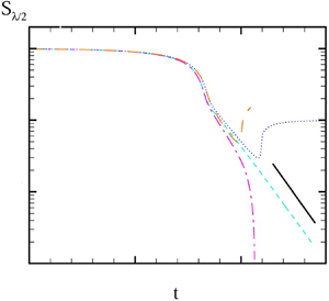
  $S_{\lambda /2}$, undergoes first a fast decrease dominated by the inertial and capillary forces, and then steps into a relatively slow decrease stage in which the elastic and capillary forces presumably play a role (Clasen et al. Reference Clasen, Eggers, Fontelos, Li and McKinley2006a). In the elasto-capillary regime, if the outer fluid phase exists, the decrease in
  $S_{\lambda /2}$ does not follow the
  $1/3De$ exponential law as in vacuum, which appears to be slightly slower. Most significantly, at some instant,
  $S_{\lambda /2}$ starts to increase, indicating that a secondary droplet is being formed at the midpoint. With the formation of the secondary droplet, the polymeric stress at the midpoint decreases rapidly, as shown in figure 4(b). Ultimately the first normal stress difference
  $\tau _{zz}-\tau _{rr}$ approaches zero and ends up with a small negative value, which is not illustrated in the semi-logarithmic plot in figure 4(b).

Figure 4. Effect of the viscosity ratio  $m_\eta$ on the evolution of the Oldroyd-B viscoelastic thread. (a) The thread radius
  $S$ at the midpoint
  $z=\lambda /2$, (b) the first normal stress difference
  $\tau _{zz}-\tau _{rr}$ at
  $z=\lambda /2$, (c) the minimum thread radius
  $S_{min}$ and (d)
  $\tau _{zz}-\tau _{rr}$ at
  $S_{min}$. Here
  $k=0.9, Oh=1.4, \beta =0.5, De=3.5, d=5, \alpha =0$.
The variation of the minimum thread radius  $S_{min}$ with time is shown in figure 4(c). Surprisingly, while the secondary droplet at the midpoint is formed, the decrease of
  $S_{min}$ gets slightly faster, with a rate slightly (about
  $2\,\%$) higher than
  $1/3De$. The polymeric stress at
  $S_{min}$ experiences an increase greater than the
  $1/3De$ law at the moment the secondary droplet begins to form, as shown in figure 4(d). After the secondary droplet is formed, the distribution of the forces along the filament, especially the capillary and elastic forces, is substantially changed.
To better understand the effect of the outer viscous fluid phase on the stretch of the thread, the force exerted on the thread by the outer fluid, expressed as  $f^{e}=-2 m_\eta Oh u^{i} G(s, d)/S^{2}$ in the 1-D momentum equation (2.17), is calculated and diagrammed in figure 5 for
  $k=0.9$,
  $m_\eta =0.04$ and three time instants
  $t=170$,
  $190$ and
  $201$, where a half-wavelength-long segment of the thread
  $z\in [0, \lambda /2]$ is plotted. At
  $t=170$, the secondary droplet at the midpoint has not been formed yet, and the thickness of the stretched filament between primary droplets is almost axially uniform. The force exerted by the outer fluid,
  $f^{e}$, is positive in the entire filament (see figure 5a), indicating that the outer fluid tends to stop fluid particles in the filament from moving towards the primary droplet and slows down the thinning of the filament, as shown in figure 4(a). That is,
  $f^{e}$ acts as a resistance to the extensional flow in the filament. This force induces the non-uniformity of the filament thickness gradually. In figure 5(b), at
  $t=190$, the non-uniformity becomes more evident, with a mild hump appearing at the midpoint. In the neighbourhood of the midpoint the elastic stress decreases dramatically to almost zero. Under the action of the capillary pressure, the small hump eventually obtains a spheroidal shape, as shown in figure 5(c). On the other hand, from the distribution of
  $f^{e}$ in the filament between the primary droplet and the hump in figure 5(b), the outer fluid still resists the thinning of the filament. At
  $t=201$, the double-fold configuration of
  $f^{e}$ indicates that another secondary droplet is going to be formed at some location. Indeed, for
  $m_\eta =0.04$, two generations of secondary droplets exist in the filament, as shown in figure 3(d). As the filament is stretched,
  $f^{e}$ is increased, but it remains as a secondary factor compared with the capillary and elastic forces. So its resisting effect on the filament thinning is quite limited all the time, as illustrated in figure 4(c).

Figure 5. The thread profile  $S$ (solid lines) and the force exerted on the thread by the outer fluid
  $f^{e}$ (dashed lines) at different instants. Here
  $k=0.9, Oh=1.4, \beta =0.5, De=3.5, m_\eta =0.01, d=5, \alpha =0$.
At smaller wavenumbers, the scenario is similar. That is, the outer viscous fluid tends to induce the formation of secondary droplets on the filament. As shown in figure 6 where the axial wavenumber  $k=0.3$, when the viscosity ratio
  $m_\eta$ is increased from 0 to 0.01, more generations of secondary droplets are produced successively. Different generations have difference sizes, and those smallest secondary droplets are hardly seen in the figure. This beads-on-a-string structure with multiple secondary droplets, described by Kamat et al. (Reference Kamat, Wagoner, Thete and Basaran2018) as micro-thread cascades, may also be induced by a surfactant or an imposed electric field (Li, Yin & Yin Reference Li, Yin and Yin2017b; Kamat et al. Reference Kamat, Wagoner, Thete and Basaran2018; Li et al. Reference Li, Ke, Yin and Yin2019). The space–time diagrams demonstrate that the necking of the thread is slowed down to a certain extent by the outer fluid phase.

Figure 6. Space–time diagrams of the evolution of the Oldroyd-B viscoelastic thread and its profile for (a)  $m_\eta =0$ and (b)
  $m_\eta =0.01$. Here
  $k=0.3, Oh=1.4, \beta =0.5, De=3.5, d=5, \alpha =0$.
The axial wavenumber  $k$ is considered to be an important parameter influencing the topological structure of a viscoelastic thread (Ardekani et al. Reference Ardekani, Sharma and Mckinley2010). We diagram the situation in the
  $(k, m_\eta )$ plane in figure 7, where for each couple of
  $k$ and
  $m_\eta$ the number of secondary droplets is counted. Generally, as
  $k$ decreases or
  $m_\eta$ increases, more secondary droplets appear in the filament between two adjacent primary droplets. Even when the viscosity of the outer fluid is very small (the smallest value of
  $m_\eta$ in the calculation is 0.001), at least one secondary droplet is formed, regardless of the value of the axial wavenumber. It seems that the appearance of secondary droplets is unavoidable in the presence of an outer viscous fluid. Differently, in the absence of an outer fluid phase, at large wavenumbers, such as
  $k=0.8$ or
  $0.9$ as shown in figure 7, there is no satellite droplet formed in beads-on-a-string structure (Ardekani et al. Reference Ardekani, Sharma and Mckinley2010; Keshavarz et al. Reference Keshavarz, Sharma, Houze, Koerner, Moore, Cotts, Threlfall-Holmes and McKinley2015). Our simulation result shows that the presence of an outer fluid phase does not favour the formation of a uniform filament that is expected in applications such as fluid bridge and extensional rheometer (Ardekani et al. Reference Ardekani, Sharma and Mckinley2010; Mathues et al. Reference Mathues, Formenti, Mcllroy, Harlen and Clasen2018; Figueiredo et al. Reference Figueiredo, Oishi, Afonso and Alves2020).

Figure 7. The statistics of secondary droplets in the ( $k, m_\eta$) plane. The numbers indicate how many secondary droplets are formed in the filament between two adjacent primary droplets. Here
  $Oh=1.4, \beta =0.5, De=3.5, d=5, \alpha =0$.
The effect of the confinement on the Oldroyd-B viscoelastic thread is examined in figure 8, where the radius ratio  $d$ varies from 2 to 10. In figures 8(a) and 8(b), two-wavelength-long thread segments are plotted for
  $k=0.3$ and
  $k=0.9$, respectively. It is shown that for all values of
  $d$ considered, the thread evolves into a quite similar beads-on-a-string structure. Not like the viscosity ratio
  $m_\eta$, the confinement hardly influences the topological structure of a fully stretched thread. In addition, a closer observation finds that as
  $d$ decreases the sizes of secondary droplets of all generations are increased slightly; see the zoomed-in plots in figures 8(a) and 8(b). That is, the confinement helps secondary droplets gain some weight.

Figure 8. Effect of the radius ratio  $d$ on the nonlinear behaviour of the Oldroyd-B viscoelastic thread. The thread profile for (a)
  $k=0.3$ and (b)
  $k=0.9$ as
  $d$ varies. The arrows denote the direction of
  $d$ increasing. The variation of (c) the minimum thread radius
  $S_{min}$ (the lower lines) and the corresponding location
  $z_{min}$ (the upper lines) and (d) the first normal stress difference
  $\tau _{zz}-\tau _{rr}$ at
  $S_{min}$ with time, where
  $k=0.9$. Here
  $Oh=1.4, \beta =0.5, De=3.5, m_\eta =0.01, \alpha =0$.
Figure 8(c) shows the time evolution of the minimum thread radius  $S_{min}$ for
  $k=0.9$, where the location of
  $S_{min}$, i.e.
  $z_{min}$ (relative to half-wavelength
  $\lambda /2$), is plotted as well. As
  $d$ decreases, the decrease of
  $S_{min}$ is slowed down, indicating that the confinement has a stabilization effect on the perturbed thread, which is well predicted by linear theory in figure 2(b). Initially,
  $S_{min}$ is located at the midpoint of the thread,
  $z_{min}/(\lambda /2)$ being equal to 1. Later, when the deformation of the thread enters the elasto-capillary stage,
  $z_{min}$ moves away from the midpoint
  $z=\lambda /2$. Ultimately,
  $S_{min}$ is located in the neck region joining the filament to the primary droplet where
  $z_{min}/(\lambda /2)\simeq 0.5$. Generally, for different values of
  $d$, the variation of
  $S_{min}$ with time is quite similar in the elasto-capillary stage. The time evolution of the first normal stress difference
  $\tau _{zz}-\tau _{rr}$ at
  $S_{min}$ is also similar for all values of
  $d$, as shown in figure 8(d).
Given the thread profile  $S$ and the axial velocity
  $u$, the force exerted by the outer fluid phase,
  $f^{e}$, is calculated for different values of the radius ratio
  $d$. The relevant results are shown in figure 9, where two typical time instants are plotted. At
  $t=179$, the thread exhibits a beads-on-a-string profile in which the secondary droplet is not formed yet (see figure 9a). The filament between primary droplets is almost axially uniform. The force exerted by the outer fluid,
  $f^{e}$, is positive in the filament (see figure 9c), which serves as a resistance to the extensional flow. As
  $d$ decreases,
  $f^{e}$ increases, indicating that the confinement enhances the influence of the outer fluid phase on the deformation of the thread. From the distribution of the axial velocity in the filament shown in figure 9(a), the extension rate
  $\partial u/\partial z$ deviates from
  $2/3De$ of an Oldroyd-B viscoelastic thread in vacuum. This is understandable, considering that
  $f^{e}$ is a resistance which decelerates the motion of fluid particles in the filament. Basically, away from the midpoint of the filament, the extension rate becomes larger. The extensional flow with a spatially varying extension rate implies that the filament thickness can no longer be uniform. Close to the primary droplet, the filament is more stretched. At the later time
  $t=200$, the secondary droplet at the midpoint is about to be shaped (see figure 9b). The distribution of the force in figure 9(d) suggests that
  $f^{e}$ is still a resistance. As
  $d$ decreases,
  $f^{e}$ increases, resulting in a larger size of secondary droplet, as shown in figure 8. In figure 9(b), the axial velocity in the filament deviates slightly from the
  $2/3De$ slope, and the trend that the extension rate varies along the axial direction suggests that the filament is most stretched in the neck regions.

Figure 9. (a,b) The thread profile  $S$ (solid lines) and the axial velocity
  $u$ (dashed lines) and (c,d) the force exerted on the thread by the outer fluid
  $f^{e}$ at two typical instants. The arrows denote the direction of
  $d$ increasing. Here
  $k=0.9, Oh=1.4, \beta =0.5, De=3.5, m_\eta =0.01, \alpha =0$.
3.3. Nonlinear behaviour of a Giesekus viscoelastic thread surrounded by a viscous fluid in a tube
For a Giesekus viscoelastic thread, breakup occurs in a finite time. It is well established that at the final stages prior to pinch-off, the minimum radius of a Giesekus viscoelastic thread approaches zero linearly with time, i.e.  $S_{min}\sim (t_p-t)$, where
  $t_p$ is the pinching time (Fontelos & Li Reference Fontelos and Li2004; Ardekani et al. Reference Ardekani, Sharma and Mckinley2010). In this study, it is found that an outer viscous fluid affects the topological structure of a Giesekus thread in a way similar to how it affects an Oldroyd-B thread. Some results are shown in figure 10.

Figure 10. Comparison of Oldroyd-B and Giesekus viscoelastic fluid threads in vacuum or surrounded by an outer viscous fluid. (a) The thread profile. (b) The time evolution of the thread radius  $S$ at the midpoint
  $z=\lambda /2$. (c) The minimum thread radius
  $S_{min}$ (the lower lines) and its location
  $z_{min}/(\lambda /2)$ (the upper lines). (d) Typical distribution of
  $\tau _{zz}-\tau _{rr}$ along the thread, where
  $z\in [0, \ \lambda /2]$. (e) The first normal stress difference
  $\tau _{zz}-\tau _{rr}$ at
  $z=\lambda /2$. (f) The extension rate
  $\dot {\varepsilon }$ at
  $z=\lambda /2$. (g) The Trouton ratio
  $\eta ^{i}_E/\eta ^{i}_0$ at
  $z=\lambda /2$. Short dashed:
  $m_\eta =0, \alpha =0$; dotted:
  $m_\eta =0.01, \alpha =0$; dash-dotted:
  $m_\eta =0, \alpha =0.005$; long dashed:
  $m_\eta =0.01, \alpha =0.005$. Here
  $k=0.8, Oh=1.4, \beta =0.5, De=3.5, d=5$.
In figure 10, four different cases, i.e. an Oldroyd-B thread in vacuum ( $m_\eta =0, \alpha =0$), an Oldroyd-B thread surrounded by a viscous fluid (
 $m_\eta =0.01, \alpha =0$), a Giesekus thread in vacuum (
 $m_\eta =0, \alpha =0.005$) and a Giesekus thread surrounded by a viscous fluid (
 $m_\eta =0.01, \alpha =0.005$), are presented for comparison. For the relatively large axial wavenumber
  $k=0.8$ considered in the figure, in the absence of the outer fluid phase, no secondary droplet is formed at the midpoint of the filament, regardless of fluid type; in the presence of an outer fluid, secondary droplets always appear in the thread, although the sizes of them are different for Oldroyd-B and Giesekus fluids, as can be seen from the thread profiles in figure 10(a). As shown in figure 10(b), the Oldroyd-B thread in vacuum necks down following the
  $1/3De$ exponential law in the elasto-capillary stage. Differently, the thickness of the Giesekus thread in vacuum decreases much more rapidly and reaches zero at
  $t_p$. In the presence of the outer viscous fluid phase,
  $S_{\lambda /2}$ of either Oldroyd-B or Giesekus thread starts to increase at some instant, indicating the formation of a secondary droplet at the midpoint. Moreover, the final
  $S_{\lambda /2}$ for the Giesekus thread is larger, indicating that its secondary droplet is larger. Fontelos & Li (Reference Fontelos and Li2004) found that due to the non-zero mobility factor
  $\alpha$, a Giesekus viscoelastic filament in vacuum may lose its uniformity. In this problem, apart from the mobility factor, the outer fluid phase is also a factor inducing the non-uniformity of the filament. Accompanied by the formation of the secondary droplet, the decrease in the minimum thread radius of both Oldroyd-B and Giesekus threads becomes a little faster than in the case of no outer fluid, as illustrated in figure 10(c).
Typical distribution of the first normal stress difference  $\tau _{zz}-\tau _{rr}$ at large times is presented in figure 10(d) for a half-wavelength-long segment of the thread. It is clear that only the polymeric stress of the Oldroyd-B thread in vacuum is axially uniform in the filament, whose growth in time follows the
  $1/3De$ exponential law, as shown in figure 10(e). The outer fluid phase induces the non-uniformity of
  $\tau _{zz}-\tau _{rr}$ in the filament of Oldroyd-B fluid, with the minimum stress located near the centre of the filament between the primary droplet at
  $z=0$ and the formed secondary droplet at
  $z=\lambda /2$. Thus the gradient of
  $\tau _{zz}-\tau _{rr}$ provides a force that tends to push fluid particles in the filament towards the primary or secondary droplet, accelerating the necking of the thread. The Giesekus thread in vacuum has the maximum
  $\tau _{zz}-\tau _{rr}$ at the midpoint of the filament
  $z=\lambda /2$. Moreover, this
  $\tau _{zz}-\tau _{rr}$ at the midpoint grows much faster than the
  $1/3De$ exponential law, as shown in figure 10(e). Away from the midpoint the polymeric stress decreases monotonically and an axially uniform distribution of it can never be built in the filament. In such a case, the filament is most stretched at the midpoint and
  $S_{min}$ coincides with
  $S_{\lambda /2}$ all the time (
 $z_{min}=\lambda /2$), as illustrated in figure 10(c). That is, for a Giesekus thread in vacuum, the midpoint of the filament is the place where the thread pinches off. Differently, in the presence of the outer fluid, the maximum
  $\tau _{zz}-\tau _{rr}$ of the Giesekus thread is located in the neck region connecting the primary droplet to the filament, which suggests that the pinch-off occurs there. Indeed, as shown in figure 10(c), its minimum radius
  $z_{min}$ moves from the midpoint towards the neck at large times and is located there eventually. Away from the neck,
  $\tau _{zz}-\tau _{rr}$ decreases monotonically, resulting in a negative gradient of polymeric stress in the filament, which tends to push fluid particles towards the primary droplet and accelerate the pinching process. In figure 10(e),
  $\tau _{zz}-\tau _{rr}$ at the midpoint of either Oldroyd-B or Giesekus thread immersed in an outer fluid phase decreases markedly to a minimal value, due to the fact that a secondary droplet is formed at the midpoint.
The extension rate  $\dot {\varepsilon }=\partial u/\partial z$ at the midpoint
  $z=\lambda /2$ is illustrated in figure 10(f) for the four cases. It is shown that in the absence of the outer fluid the Giesekus thread has an extension rate much higher than the Oldroyd-B thread whose value is maintained at
  $2/3De$. Figure 10(g) shows the Trouton ratio defined as
  $\eta ^{i}_E/\eta ^{i}_0=3\beta +(\tau _{zz}-\tau _{rr})/Oh\dot {\varepsilon }$, where
  $\eta ^{i}_E$ is the transient extensional viscosity (Ardekani et al. Reference Ardekani, Sharma and Mckinley2010). Only for the Oldroyd-B thread in vacuum does the extensional viscosity grow almost exponentially. In contrast, the extensional viscosity of the Giesekus thread in vacuum stays moderate when pinch-off occurs. In the presence of the outer fluid, the Oldroyd-B or Giesekus thread may experience a sharp increase in the Trouton ratio just before the formation of secondary droplet, as shown in figure 10(g). Then, with the formation of a secondary drop at the midpoint, the extensional viscosity there ceases to increase. Instead, the Trouton ratio decreases rapidly and ends up with a small negative value at the moment the secondary droplet is formed (the decrease and the negative values are not shown in the semi-logarithmic plot of figure 10g).
More space–time diagrams of the evolution of the thread are shown in figure 11, where the axial wavenumber  $k$ is fixed at a relatively small value of 0.5. For this relatively long wave, a secondary droplet appears at the midpoint of the Oldroyd-B thread in vacuum, as shown in figure 11(a). When
  $\alpha$ is increased from 0 to 0.005, the secondary droplet at the midpoint is maintained but its size is decreased, as shown in figure 11(b). Comparing the space–time diagrams in figures 11(a) and 11(b), the Giesekus thread necks down much faster than the Oldroyd-B thread. On the other hand, for the Giesekus thread, at the final stages prior to pinch-off, the filament between the primary and secondary droplets becomes non-uniform. In figure 11(c), where the viscosity ratio
  $m_\eta$ is increased from 0 to 0.01, the non-uniformity of the filament becomes more pronounced, with the aid of the outer fluid, which can be seen from the profile on the right-hand side. Meanwhile, the secondary droplet becomes larger.

Figure 11. Space–time diagrams of the deformation of the Oldroyd-B or Giesekus viscoelastic thread and the final profiles for (a)  $\alpha =0, m_\eta =0$, (b)
  $\alpha =0.005, m_\eta =0$ and (c)
  $\alpha =0.005, m_\eta =0.01$. Here
  $k=0.5, Oh=1.4, \beta =0.5, De=3.5, d=5$.
4. Conclusion
Based on the slender body theory, a 1-D model is built for a two-phase flow system, in which an infinitely long viscoelastic fluid thread is surrounded by a Newtonian viscous fluid layer confined in a coaxial cylindrical tube. The viscoelasticity of the inner fluid is described by the Oldroyd-B or Giesekus constitutive equation, and the outer fluid is assumed to be much lighter and much less viscous than the inner fluid. Under such an assumption, the 1-D equations are successfully derived. The effect of the outer viscous fluid phase and the confinement of the tube on the evolution of the beads-on-a-string structure of the viscoelastic thread is examined by numerically solving the nonlinear 1-D equations. Direct simulations and experimental observations will be hopefully carried out in the future to compare with and confirm the 1-D predictions obtained in this work.
In the 1-D model, there are two dimensionless parameters related to the outer fluid or the confinement, i.e. the outer to inner fluid viscosity ratio  $m_\eta$ and the tube to thread radius ratio
  $d$. For an Oldroyd-B viscoelastic thread, it is found that the presence of the outer viscous fluid phase may lead to the formation of secondary droplets on the filament between two adjacent primary droplets, even for large wavenumbers. For a fixed wavenumber, as
  $m_\eta$ increases, more and more secondary droplets appear in the filament, and meanwhile those existing secondary droplets get larger. The outer viscous fluid exerts a resistance force on the filament, which tends to resist the stretching of the thread. On the other hand, due to the formation of secondary droplets, the capillary and elastic forces are redistributed in the filament, and the polymeric stress loses its uniformity. As a result, the necking of the thread gets slightly faster than in the case of no outer fluid phase. Decreasing the radius ratio
  $d$ results in an increase in secondary droplet size, but affects little the topological structures of viscoelastic threads.
At sufficiently large wavenumbers, secondary droplets are absent from a Giesekus thread in vacuum, and the thread pinches off at the midpoint of the filament between primary droplets, where the polymeric stress is maximal. In contrast, in the presence of an outer viscous phase, secondary droplets are formed and pinch-off occurs in the neck region connecting the filament to the primary droplet, where the thread is most stressed. Moreover, as  $m_\eta$ increases, the non-uniformity of the filament thickness becomes more and more pronounced.
In addition, a simple linear analysis is executed. The dispersion relations for the 1-D model as well as for the 2-D axisymmetric instability are obtained. It is shown that the mobility factor of the Giesekus model is a secondary factor in linear instability. Increasing  $m_\eta$ or decreasing
  $d$ may suppress the instability of the viscoelastic thread. The 1-D slender body approximation predicts well the linear instability of the thread at small wavenumbers.
Viscoelasticity influences the linear instability and nonlinear evolution of a viscoelastic thread to a great extent. In this 1-D analysis, the fluid is limited to being of high viscoelasticity (the values of the Ohnesorge and Deborah numbers are relatively large). The present study illuminates just a part of the whole picture. It would be of interest to expand the ranges of the non-dimensional parameters in future 1-D or 2-D numerical simulations.
Acknowledgements
The authors would like to thank Professor J.J. Wylie from City University of Hong Kong for his careful reading of the manuscript and useful suggestions.
Funding
F.L. was supported by the National Natural Science Foundation of China (nos. 11772328 and 11621202). D.H. was supported by the president's fund–research start-up fund from the Chinese University of Hong Kong, Shenzhen (PF01000857) and the National Natural Science Foundation of China (No. 12172317).
Declaration of interests
The authors report no conflict of interest.
Appendix A. Derivation of the 1-D model
In the 1-D model, the thread is assumed to be perturbed by a small cosinoidal harmonic at the initial time. Naturally, the radius of the unperturbed thread  $R$ is the characteristic length in the radial direction (
 $l_r$) and the wavelength of the perturbation
  ${2{\rm \pi} }/{k}$ is the characteristic length in the axial direction (
 $l_z$). Apparently, within the range of the wavenumber
  $k$ considered,
  $l_r$ is much smaller than
  $l_z$, i.e.
 \begin{equation} l_r=\varepsilon l_z, \end{equation}
where  $\varepsilon$ is a small parameter. In such a case, the slender body theory can be applied.
The balance of capillary, inertial and viscoelastic forces of the inner fluid gives
 \begin{equation} \rho^{i}\frac{l_z}{l^{2}_t}=\eta^{i}_0\frac{l_z/l_t}{l^{2}_z}=\frac{\sigma}{l_r}\frac{1}{l_z}. \end{equation}
Using the scales
 \begin{align} \left.\begin{array}{c@{}} \displaystyle r=l_r\tilde{r},\ z=l_z\tilde{z}, \ t=l_t\tilde{t}, \ S=l_r\tilde{S}, \ d=l_r\tilde{d},\ v^{i}=\dfrac{l_r}{l_t}\tilde{v}^{i}, v^{e}=\dfrac{l_r}{l_t}\tilde{v}^{e}, \ u^{i}=\dfrac{l_z}{l_t}\tilde{u}^{i}, \ u^{e}=\dfrac{l_z}{l_t}\tilde{u}^{e}, \\ \displaystyle p^{i}=\dfrac{\rho^{i}l^{2}_z}{l^{2}_t}\tilde{p}^{i},\ p^{e}=\dfrac{\rho^{i}l^{2}_z}{l^{2}_t}\tilde{p}^{e},\ \tau_{rr}=\dfrac{\rho^{i}l^{2}_z}{l^{2}_t}\tilde{\tau}_{rr},\ \tau_{\theta\theta}=\dfrac{\rho^{i}l^{2}_z}{l^{2}_t}\tilde{\tau}_{\theta\theta}, \ \tau_{zz}=\dfrac{\rho^{i}l^{2}_z}{l^{2}_t}\tilde{\tau}_{zz},\ \tau_{rz}=\dfrac{\rho^{i}l^{3}_z}{l_rl^{2}_t}\tilde{\tau}_{rz}, \end{array}\right\} \end{align}
where the tilde denotes the corresponding non-dimensional quantities, and omitting the tildes, one can get the following non-dimensionalized governing equations and boundary conditions.
For the inner viscoelastic fluid:
 \begin{gather} \frac{1}{r}\frac{\partial(rv^{i})}{\partial r}+\frac{\partial u^{i}}{\partial z}=0, \end{gather}
 \begin{align} \frac{\partial v^{i}}{\partial t}+v^{i}\frac{\partial v^{i}}{\partial r}+u^{i}\frac{\partial v^{i}}{\partial z}&={-}\frac{1}{\varepsilon^{2}}\frac{\partial p^{i}}{\partial r}+\frac{\beta}{\varepsilon^{2}}\left(\frac{\partial^{2}v^{i}}{\partial r^{2}}+\frac{1}{r}\frac{\partial v^{i}}{\partial r}-\frac{v^{i}}{r^{2}}\right)+\beta \frac{\partial^{2}v^{i}}{\partial z^{2}}\nonumber\\ &\quad +\frac{1}{\varepsilon^{2}}\left(\frac{\partial \tau_{rr}}{\partial r}+\frac{\partial \tau_{rz}}{\partial z}+\frac{\tau_{rr}-\tau_{\theta\theta}}{r}\right), \end{align}
 \begin{align} \frac{\partial u^{i}}{\partial t}+v^{i}\frac{\partial u^{i}}{\partial r}+u^{i}\frac{\partial u^{i}}{\partial z}&={-}\frac{\partial p^{i}}{\partial z}+\frac{\beta}{\varepsilon^{2}}\left(\frac{\partial^{2}u^{i}}{\partial r^{2}}+\frac{1}{r}\frac{\partial u^{i}}{\partial r}\right)\nonumber\\&\quad +\beta \frac{\partial^{2}u^{i}}{\partial z^{2}}+\frac{1}{\varepsilon^{2}}\frac{\partial \tau_{rz}}{\partial r}+\frac{1}{\varepsilon^{2}}\frac{\tau_{rz}}{r}+\frac{\partial \tau_{zz}}{\partial z}, \end{align}
 \begin{align} &\tau_{rr}+De\left(\frac{\partial \tau_{rr}}{\partial t}+v^{i}\frac{\partial \tau_{rr}}{\partial r}+u^{i}\frac{\partial \tau_{rr}}{\partial z}-2\tau_{rr}\frac{\partial v^{i}}{\partial r}-2\tau_{rz}\frac{\partial v^{i}}{\partial z}\right)\nonumber\\ &\quad +\frac{\alpha De}{1-\beta}\left(\tau^{2}_{rr}+\frac{1}{\varepsilon^{2}}\tau^{2}_{rz}\right) =2(1-\beta)\frac{\partial v^{i}}{\partial r}, \end{align}
 \begin{gather} \tau_{\theta\theta}+De\left(\frac{\partial \tau_{\theta\theta}}{\partial t}+v^{i}\frac{\partial \tau_{\theta\theta}}{\partial r}+u^{i}\frac{\partial \tau_{\theta\theta}}{\partial z}-2\tau_{\theta\theta}\frac{v^{i}}{r}\right)+\frac{\alpha De}{1-\beta}\tau^{2}_{\theta\theta}=2(1-\beta)\frac{v^{i}}{ r},\end{gather}
 \begin{align} &\tau_{zz}+De\left(\frac{\partial \tau_{zz}}{\partial t}+v^{i}\frac{\partial \tau_{zz}}{\partial r}+u^{i}\frac{\partial \tau_{zz}}{\partial z}-\frac{2}{\varepsilon^{2}}\tau_{rz}\frac{\partial u^{i}}{\partial r}-2\tau_{zz}\frac{\partial u^{i}}{\partial z}\right)\nonumber\\ &\quad +\frac{\alpha De}{1-\beta}(\tau^{2}_{zz}+\tau^{2}_{rz}) =2(1-\beta)\frac{\partial u^{i}}{ \partial z}, \end{align}
 \begin{align} &\tau_{rz}+De\left(\frac{\partial \tau_{rz}}{\partial t}+v^{i}\frac{\partial \tau_{rz}}{\partial r}+u^{i}\frac{\partial \tau_{rz}}{\partial z}+\frac{v^{i}}{r}\tau_{rz}-\tau_{rr}\frac{\partial u^{i}}{\partial r}-\varepsilon^{2}\tau_{zz}\frac{\partial v^{i}}{\partial z}\right)\nonumber\\ &\quad +\frac{\alpha De}{1-\beta}(\tau_{rr}+\tau_{zz})\tau_{rz} =(1-\beta)\left(\varepsilon^{2}\frac{\partial v^{i}}{\partial z}+\frac{\partial u^{i}}{\partial r}\right), \end{align}
where  $\tau _{\theta \theta }$ and
  $\tau _{rz}$ are the
  $\theta \theta$ and
  $rz$ components of the polymer stress
  $\boldsymbol{\mathsf{T}}_\textit {{p}}$,
  $De={\lambda ^{i}}/{l_t}$ and
  $\beta ={\eta ^{i}_s}/{\eta ^{i}_0}$.
For the outer Newtonian fluid:
 $$\begin{gather} \frac{1}{r}\frac{\partial(rv^{e})}{\partial r} + \frac{\partial u^{e}}{\partial z}=0, \end{gather}$$
 $$\begin{gather}m_{\rho}\left(\frac{\partial v^{e}}{\partial t}+v^{e}\frac{\partial v^{e}}{\partial r}+u^{e}\frac{\partial v^{e}}{\partial z}\right)={-}\frac{1}{\varepsilon^{2}}\frac{\partial p^{e}}{\partial r}+m_{\eta}\left(\frac{1}{\varepsilon^{2}}\left(\frac{\partial^{2}v^{e}}{\partial r^{2}}+\frac{1}{r}\frac{\partial v^{e}}{\partial r}-\frac{v^{e}}{r^{2}}\right)+ \frac{\partial^{2}v^{e}}{\partial z^{2}}\right), \end{gather}$$
 $$\begin{gather}m_{\rho}\left(\frac{\partial u^{e}}{\partial t}+v^{e}\frac{\partial u^{e}}{\partial r}+u^{e}\frac{\partial u^{e}}{\partial z}\right)={-}\frac{\partial p^{e}}{\partial z}+m_{\eta}\left(\frac{1}{\varepsilon^{2}}\left(\frac{\partial^{2}u^{e}}{\partial r^{2}}+\frac{1}{r}\frac{\partial u^{e}}{\partial r}\right)+\frac{\partial^{2} u^{e}}{\partial z^{2}}\right), \end{gather}$$
where  $m_{\rho }={\rho ^{e}}/{\rho ^{i}}$ and
  $m_{\eta }={\eta ^{e}_0}/{\eta ^{i}_0}$.
On the interface  $r=S(z,t)$, the normal dynamic balance is
 \begin{align} p^{i}&=p^{e}-\frac{2m_{\eta}}{1+\varepsilon^{2}\left(\dfrac{\partial S}{\partial z}\right)^{2}}\left(\frac{\partial v^{e}}{\partial r}-\frac{\partial S}{\partial z}\left(\frac{\partial v^{e}}{\partial z}+\frac{\partial u^{e}}{\partial r}\right)+\left(\frac{\partial S}{\partial z}\right)^{2}\frac{\partial u^{e}}{\partial z}\right)\nonumber\\ &\quad +\frac{2\beta}{1+\varepsilon^{2}\left(\dfrac{\partial S}{\partial z}\right)^{2}}\left(\frac{\partial v^{i}}{\partial r}-\frac{\partial S}{\partial z}\left(\varepsilon^{2}\frac{\partial v^{i}}{\partial z}+\frac{\partial u^{i}}{\partial r}\right)+\varepsilon^{2}\left(\frac{\partial S}{\partial z}\right)^{2}\frac{\partial u^{i}}{\partial z}\right)\nonumber\\ &\quad +\frac{1}{1+\varepsilon^{2}\left(\dfrac{\partial S}{\partial z}\right)^{2}}\left(\varepsilon^{2}\left(\frac{\partial S}{\partial z}\right)^{2}\tau_{zz}-2\frac{\partial S}{\partial z}\tau_{rz}+\tau_{rr}\right)\nonumber\\ &\quad +\frac{1}{S\left(1+\varepsilon^{2}\left(\dfrac{\partial S}{\partial z}\right)^{2}\right)^{{1}/{2}}}-\frac{\varepsilon^{2}\dfrac{\partial^{2}S}{\partial z^{2}}}{\left(1+\varepsilon^{2}\left(\dfrac{\partial S}{\partial z}\right)^{2}\right)^{3/2}}, \end{align}
the tangential force balance is
 \begin{align}
&\frac{1}{1+\varepsilon^{2}\left(\dfrac{\partial
S}{\partial z}\right)^{2}}
\left(2\beta\varepsilon^{2}\frac{\partial S}{\partial
z}\left(\frac{\partial v^{i}}{\partial r}-\frac{\partial
u^{i}}{\partial
z}\right)+\beta\left(1-\varepsilon^{2}\left(\frac{\partial
S}{\partial
z}\right)^{2}\right)\left(\varepsilon^{2}\frac{\partial
v^{i}}{\partial z}+\frac{\partial u^{i}}{\partial
r}\right)\right) \nonumber\\ &\qquad
+\frac{1}{1+\varepsilon^{2}\left(\dfrac{\partial
S}{\partial
z}\right)^{2}}\left(\varepsilon^{2}\frac{\partial
S}{\partial z}(\tau_{rr}-\tau_{zz})
+\left(1-\varepsilon^{2}\left(\frac{\partial S}{\partial
z}\right)^{2}\right)\tau_{rz}\right) \nonumber\\ &\quad
=\frac{1}{1+\varepsilon^{2}\left(\dfrac{\partial
S}{\partial z}\right)^{2}}\left(2m_{\eta}\frac{\partial
S}{\partial z}\varepsilon^{2}\left(\frac{\partial
v^{e}}{\partial r}-\frac{\partial u^{e}}{\partial
z}\right) \right.\nonumber\\ &\left.\qquad +m_{\eta}\left(1-\varepsilon^{2}\left(\frac{\partial
S}{\partial
z}\right)^{2}\right)\left(\varepsilon^{2}\frac{\partial
v^{e}}{\partial z}+\frac{\partial u^{e}}{\partial
r}\right)\right), \end{align}
\begin{align}
&\frac{1}{1+\varepsilon^{2}\left(\dfrac{\partial
S}{\partial z}\right)^{2}}
\left(2\beta\varepsilon^{2}\frac{\partial S}{\partial
z}\left(\frac{\partial v^{i}}{\partial r}-\frac{\partial
u^{i}}{\partial
z}\right)+\beta\left(1-\varepsilon^{2}\left(\frac{\partial
S}{\partial
z}\right)^{2}\right)\left(\varepsilon^{2}\frac{\partial
v^{i}}{\partial z}+\frac{\partial u^{i}}{\partial
r}\right)\right) \nonumber\\ &\qquad
+\frac{1}{1+\varepsilon^{2}\left(\dfrac{\partial
S}{\partial
z}\right)^{2}}\left(\varepsilon^{2}\frac{\partial
S}{\partial z}(\tau_{rr}-\tau_{zz})
+\left(1-\varepsilon^{2}\left(\frac{\partial S}{\partial
z}\right)^{2}\right)\tau_{rz}\right) \nonumber\\ &\quad
=\frac{1}{1+\varepsilon^{2}\left(\dfrac{\partial
S}{\partial z}\right)^{2}}\left(2m_{\eta}\frac{\partial
S}{\partial z}\varepsilon^{2}\left(\frac{\partial
v^{e}}{\partial r}-\frac{\partial u^{e}}{\partial
z}\right) \right.\nonumber\\ &\left.\qquad +m_{\eta}\left(1-\varepsilon^{2}\left(\frac{\partial
S}{\partial
z}\right)^{2}\right)\left(\varepsilon^{2}\frac{\partial
v^{e}}{\partial z}+\frac{\partial u^{e}}{\partial
r}\right)\right), \end{align}
the kinematic boundary condition is
 \begin{equation} v^{i}=\frac{\partial S}{\partial t}+u^{i}\frac{\partial S}{\partial z}\end{equation}
and the continuity of velocity requires
 \begin{equation} u^{i}=u^{e} \quad \textrm{and}\quad v^{i}=v^{e}. \end{equation}
The boundary conditions on the tube wall are
 \begin{equation} u^{e}(d,z,t)=v^{e}(d,z,t)=0.\end{equation}
 Now we expand the quantities into Taylor series of  $\varepsilon r$. For the inner viscoelastic thread:
 $$\begin{gather} u^{i}(r,z,t)=u^{i}_0(z,t)+u^{i}_2(z,t)\frac{(\varepsilon r)^{2}}{2}+\cdots, \end{gather}$$
 $$\begin{gather}v^{i}(r,z,t)={-}\frac{r}{2}\frac{\partial u^{i}_0}{\partial z}-\frac{\varepsilon^{2}r^{3}}{8}\frac{\partial u^{i}_2(z,t)}{\partial z}+\cdots, \end{gather}$$
 $$\begin{gather}p^{i}(r,z,t)=p^{i}_0(z,t)+p^{i}_2(z,t)(\varepsilon r)^{2}+\cdots, \end{gather}$$
 $$\begin{gather}\tau_{rr}(r,z,t)=\tau_{rr0}(z,t)+\tau_{rr2}(z,t)(\varepsilon r)^{2}+\cdots, \end{gather}$$
 $$\begin{gather}\tau_{zz}(r,z,t)=\tau_{zz0}(z,t)+\tau_{zz2}(z,t)(\varepsilon r)^{2}+\cdots, \end{gather}$$
 $$\begin{gather}\tau_{\theta\theta}(r,z,t)=\tau_{\theta\theta 0}(z,t)+\tau_{\theta\theta 2}(z,t)(\varepsilon r)^{2}+\cdots, \end{gather}$$
 $$\begin{gather}r\tau_{rz}(r,z,t)=\tau_{rz0}(z,t)+\tau_{rz2}(z,t)(\varepsilon r)^{2}+\cdots. \end{gather}$$
For the outer Newtonian fluid:
 $$\begin{gather} u^{e}(r,z,t)=u^{e}_0(r,z,t)+u^{e}_2(r,z,t)\varepsilon^{2}+\cdots, \end{gather}$$
 $$\begin{gather}v^{e}(r,z,t)=v^{e}_0(r,z,t)+v^{e}_2(r,z,t)\varepsilon^{2}+\cdots, \end{gather}$$
 $$\begin{gather}p^{e}(r,z,t)=p^{e}_0(r,z,t)+p^{e}_2(r,z,t)\varepsilon^{2}+\cdots. \end{gather}$$
Substituting the expansions (A19)–(A28) into the kinematic condition (A16), the leading order yields
 \begin{equation} v^{i}_0(S,z,t)=\frac{\partial S}{\partial t}+u^{i}_0\frac{\partial S}{\partial z}={-}\frac{S}{2}\frac{\partial u^{i}_0}{\partial z}. \end{equation}
This gives
 \begin{equation} \frac{\partial(S^{2})}{\partial t}+\frac{\partial(S^{2}u^{i}_0)}{\partial z}=0. \end{equation}
 Substituting the expansions into (A4)–(A10), one has  $\tau _{rz0}=0, \tau _{rr0}=\tau _{\theta \theta 0}$ and
 $$\begin{gather} \frac{\partial u^{i}_0}{\partial t}+u^{i}_0\frac{\partial u^{i}_0}{\partial z}={-}\frac{\partial p^{i}_0}{\partial z}+\beta \left(2u^{i}_2+\frac{\partial^{2} u^{i}_0}{\partial z^{2}}\right)+2\tau_{rz2}+\frac{\partial \tau_{zz0}}{\partial z}, \end{gather}$$
 $$\begin{gather}\tau_{rr0}+De\left(\frac{\partial \tau_{rr0}}{\partial t}+u^{i}_0\frac{\partial \tau_{rr0}}{\partial z}+\tau_{rr0}\frac{\partial u^{i}_0}{\partial z}\right)+\frac{\alpha De}{1-\beta}\tau^{2}_{rr0}={-}(1-\beta)\frac{\partial u^{i}_0}{\partial z}, \end{gather}$$
 $$\begin{gather}\tau_{zz0}+De\left(\frac{\partial \tau_{zz0}}{\partial t}+u^{i}_0\frac{\partial \tau_{zz0}}{\partial z}-2\tau_{zz0}\frac{\partial u^{i}_0}{\partial z}\right)+\frac{\alpha De}{1-\beta}\tau^{2}_{zz0}=2(1-\beta)\frac{\partial u^{i}_0}{\partial z}, \end{gather}$$
 $$\begin{gather}\tau_{\theta\theta 0}+De\left(\frac{\partial \tau_{\theta\theta 0}}{\partial t}+u^{i}_0\frac{\partial \tau_{\theta\theta 0}}{\partial z}-2\tau_{\theta\theta 0}\frac{\partial u^{i}_0}{\partial z}\right)+\frac{\alpha De}{1-\beta}\tau^{2}_{\theta\theta 0}={-}(1-\beta)\frac{\partial u^{i}_0}{\partial z}, \end{gather}$$
 \begin{gather} \tau_{rz2}+De\left(\frac{\partial \tau_{rz2}}{\partial t}-\tau_{rz2}\frac{\partial u^{i}_0}{\partial z}+u^{i}_0\frac{\partial \tau_{rz2}}{\partial z}-\tau_{rr0}u^{i}_2+\frac{1}{2}\tau_{zz0}\frac{\partial^{2} u^{i}_0}{\partial z^{2}}\right) \nonumber\\ +\frac{\alpha De}{1-\beta}(\tau_{rr0}+\tau_{zz0})\tau_{rz2} =(1-\beta)\left(u^{i}_2-\frac{1}{2}\frac{\partial^{2} u^{i}_0}{\partial z^{2}}\right). \end{gather}
 Assume that  $m_{\rho }={\rho ^{e}}/{\rho ^{i}}\sim O(\varepsilon )$ and
  $m_{\eta }={\eta ^{e}_0}/{\eta ^{i}_0}\sim O(\varepsilon ^{2})=\lambda _0\varepsilon ^{2}$, where
  $\lambda _0$ is a constant of
  $O(1)$. Equation (A12) at
  $O({1}/{\varepsilon ^{2}})$ gives
 \begin{equation} \frac{\partial p^{e}_0}{\partial r}=0, \end{equation}
which implies that  $p^{e}_0=p^{e}_0(z,t)$. Equation (A13) at
  $O(1)$ gives
 \begin{equation} -\frac{\partial p^{e}_0}{\partial z}+\lambda_0\frac{1}{r}\frac{\partial\left(r\dfrac{\partial u^{e}}{\partial r}\right)}{\partial r}=0, \end{equation}
and then we obtain
 \begin{equation} u^{e}_0=\frac{r^{2}}{4\lambda_0}\frac{\partial p^{e}_0}{\partial z}+A(z,t)\ln r+B(z,t),\end{equation}
where  $A(z,t)$ and
  $B(z,t)$ are functions of
  $z$ and
  $t$ to be determined.
From (A11) and (A38), one can obtain
 \begin{equation} v^{e}_0={-}\frac{r^{3}}{16\lambda_0}\frac{\partial^{2} p^{e}_0}{\partial z^{2}}+\frac{\partial A}{\partial z}\left(\frac{r}{4}-\frac{r\ln r}{2}\right)-\frac{\partial B}{\partial z}\frac{r}{2}+\frac{C}{r}.\end{equation}
From (A18), one has
 $$\begin{gather} B={-}\frac{d^{2}}{4\lambda_0}\frac{\partial p^{e}_0}{\partial z}-A\ln d, \end{gather}$$
 $$\begin{gather}C=\frac{d^{4}}{16\lambda_0}\frac{\partial^{2} p^{e}_0}{\partial z^{2}}-\frac{\partial A}{\partial z}\left(\frac{d^{2}}{4}-\frac{d^{2}\ln d}{2}\right)+\frac{\partial B}{\partial z}\frac{d^{2}}{2}. \end{gather}$$
Therefore, (A 17) yields
 $$\begin{gather} u^{e}_0=\frac{r^{2}-d^{2}}{4\lambda_0}\frac{\partial p^{e}_0}{\partial z}+A\ln \frac{r}{d}, \end{gather}$$
 $$\begin{gather}v^{e}_0={-}\frac{1}{\lambda_0}\left(\frac{(r^{2}-d^{2})^{2}}{16r}\frac{\partial^{2} p^{e}_0}{\partial z^{2}}+\lambda_0\frac{2r^{2}\ln \dfrac{r}{d}+d^{2}-r^{2}}{4r}\frac{\partial A}{\partial z}\right). \end{gather}$$
Thus
 \begin{equation} u^{i}_0(z,t)=u^{i}_0|_{r=S}=u^{e}_0(S,z,t)=\frac{S^{2}-d^{2}}{4\lambda_0}\frac{\partial p^{e}_0}{\partial z}+A\ln \frac{S}{d}. \end{equation}
From (A4), one has
 \begin{equation} v^{i}_0={-}\frac{r}{2}\frac{\partial u^{i}_0}{\partial z}. \end{equation}
Thus
 \begin{equation} v^{i}_0(S,z,t)=\left.\left(-\frac{r}{2}\frac{\partial u^{i}_0}{\partial z}\right)\right|_{r=S}={-}\frac{S}{2}\left(\frac{S^{2}-d^{2}}{4\lambda_0}\frac{\partial p^{e}_0}{\partial z}+A\ln \frac{S}{d}\right)_z. \end{equation}
On the other hand,
 \begin{equation} v^{e}_0(S,z,t)={-}\frac{1}{\lambda_0}\left(\frac{(S^{2}-d^{2})^{2}}{16r}\frac{\partial^{2} p^{e}_0}{\partial z^{2}}+\lambda_0\frac{2S^{2}\ln \dfrac{S}{d}+d^{2}-S^{2}}{4S}\frac{\partial A}{\partial z}\right).\end{equation}
Equations (A45) and (A47) together with (A 17) yield
 \begin{equation} A={-}\frac{S^{2}+d^{2}}{4\lambda_0}\frac{\partial p^{e}_2}{\partial z}+\frac{f(t)}{(S^{2}-d^{2})\lambda_0}, \end{equation}
where  $f(t)$ is an arbitrary function of time
  $t$.
$t$.
Thus, (A44) further gives
 \begin{equation} \frac{\partial p^{e}_2}{\partial z}=\frac{\lambda_0u^{i}_0-\dfrac{f(t)}{S^{2}-d^{2}}\ln\dfrac{S}{d}}{\dfrac{S^{2}-d^{2}}{4} -\dfrac{S^{2}+d^{2}}{4}\ln\dfrac{S}{d}}.\end{equation}
 The normal condition (A14) at  $O(1)$ together with (A19) and (A45) yields
 \begin{equation} p^{i}_0=p^{e}_0-\beta \frac{\partial u^{i}_0}{\partial z}+\tau_{rr0}+\hat{\kappa} \end{equation}
and
 \begin{equation} \frac{\partial p^{i}_0}{\partial z}=\frac{\partial p^{e}_0}{\partial z}-\beta \frac{\partial^{2} u^{i}_0}{\partial z^{2}}+\frac{\partial \tau_{rr0}}{\partial z}+\frac{\partial \hat{\kappa}}{\partial z}, \end{equation}
where
 \begin{equation} \hat{\kappa}=\frac{1}{S\left(1+\varepsilon^{2}\left(\dfrac{\partial S}{\partial z}\right)^{2}\right)}-\frac{\varepsilon^{2} \dfrac{\partial^{2} S}{\partial z^{2}}}{\left(1+\varepsilon^{2}\left(\dfrac{\partial S}{\partial z}\right)^{2}\right)^{3/2}}. \end{equation}
 The tangential condition (A15) at  $O(\varepsilon ^{2})$ together with (A19), (A42) and (A45) gives
 \begin{align} {-}3\beta \frac{\partial S}{\partial z}\frac{\partial u^{i}_0}{\partial z}+\beta \frac{\partial v^{i}_0}{\partial z}+S \left(\beta u^{i}_2+\tau_{rz2}\right)+\frac{\partial S}{\partial z}\left(\tau_{rr0}-\tau_{zz0}\right)=\frac{S^{2}-d^{2}}{4S}\frac{\partial p^{e}_0}{\partial z}+\frac{f(t)}{S(S^{2}-d^{2})}. \end{align}
Equation (A6) at O(1) gives
 \begin{equation} \frac{\partial u^{i}_0}{\partial t}+u^{i}_0\frac{\partial u^{i}_0}{\partial z}={-}\frac{\partial p^{i}_0}{\partial z}+2\left(\beta u^{i}_2+\tau_{rz2}\right)+\beta \frac{\partial^{2} u^{i}_0}{\partial z^{2}}+\frac{\partial \tau_{zz0}}{\partial z}. \end{equation}
Using (A49), (A51), (A53) and (A54), one can obtain
 \begin{align} &\frac{\partial u^{i}_0}{\partial t}+u^{i}_0\frac{\partial u^{i}_0}{\partial z}=\frac{\beta}{S^{2}}\frac{\partial\left(3S^{2}\dfrac{\partial u^{i}_0}{\partial z}\right)}{\partial z}+\frac{1}{S^{2}}\frac{\partial\left(S^{2}\left(\tau_{zz0}-\tau_{rr0}\right)\right)}{\partial z}\nonumber\\ &\quad -\frac{\partial \hat{\kappa}}{\partial z}-\frac{2}{S^{2}}\left(\lambda_0u^{i}_0-\frac{f(t)}{S^{2}+d^{2}}\right)G(S,d), \end{align}
where
 \begin{equation} G(S,d)=\frac{S^{2}+d^{2}}{S^{2}-d^{2}-(S^{2}+d^{2})\ln \dfrac{S}{d}}. \end{equation}
Equations (A30), (A32), (A33) and (A55) constitute the 1-D model. For brevity we drop the superscript  $i$ and the subscript 0.
Note that in this problem the shape of the stretched thread is spatially periodic in the  $z$ direction. Being a cosinoidal harmonic perturbation imposed on the thread at the initial time (Wang Reference Wang2013), one has
 \begin{equation} f(t)=\frac{\displaystyle \int^{{\lambda}/{2}}_{-{\lambda}/{2}}S^{2}\left(\frac{\partial u^{i}}{\partial t}+u^{i}\frac{\partial u^{i}}{\partial z}\right)\, \textrm{d} z+2\lambda_0\int^{{\lambda}/{2}}_{-{\lambda}/{2}}u^{i}G(S,d)\, \textrm{d} z}{\displaystyle \int^{{\lambda}/{2}}_{-{\lambda}/{2}}\frac{2G(S,d)}{S^{2}+d^{2}}\, \textrm{d} z}=0, \end{equation}
where  $\lambda ={2{\rm \pi} }/{kR}$ is the dimensionless wavelength of the perturbation.
Now one can write the above 1-D equations in the following dimensional form:
 $$\begin{gather} \frac{\partial(S^{2})}{\partial t}+\frac{\partial(S^{2}u^{i})}{\partial z}=0, \end{gather}$$
 $$\begin{gather}\rho^{i}\left(\frac{\partial u^{i}}{\partial t}+u^{i}\frac{\partial u^{i}}{\partial z}\right)=\frac{3\eta^{i}_s}{S^{2}}\frac{\partial\left(S^{2}\dfrac{\partial u^{i}}{\partial z}\right)}{\partial z}+\frac{1}{S^{2}}\frac{\partial(S^{2}(\tau_{zz}-\tau_{rr}))}{\partial z}-\sigma\frac{\partial \kappa}{\partial z}-\frac{2}{S^{2}}\eta^{e}_0u^{i}G(S,R_0), \end{gather}$$
 $$\begin{gather}\tau_{zz}+\lambda^{i}\left(\frac{\partial \tau_{zz}}{\partial t}+u^{i}\frac{\partial \tau_{zz}}{\partial z}-2\tau_{zz}\frac{\partial u^{i}}{\partial z}\right)+\frac{\alpha \lambda^{i}}{\eta^{i}_p}\tau^{2}_{zz}=2\eta^{i}_p\frac{\partial u^{i}}{\partial z}, \end{gather}$$
 $$\begin{gather}\tau_{rr}+\lambda^{i}\left(\frac{\partial \tau_{rr}}{\partial t}+u^{i}\frac{\partial \tau_{rr}}{\partial z}+\tau_{rr}\frac{\partial u^{i}}{\partial z}\right)+\frac{\alpha \lambda^{i}}{\eta^{i}_p}\tau^{2}_{rr}={-}\eta^{i}_p\frac{\partial u^{i}}{\partial z}, \end{gather}$$
where
 \begin{align} G(S,R_0)=\frac{S^{2}+R^{2}_0}{S^{2}-R^{2}_0-(S^{2}+R^{2}_0)\ln \dfrac{S}{R_0}},\enspace \kappa=\frac{1}{S\left(1+\left(\dfrac{\partial S}{\partial z}\right)^{2}\right)^{{1}/{2}}}-\frac{\dfrac{\partial^{2}S}{\partial z^{2}}}{\left(1\!+\!\left(\dfrac{\partial S}{\partial z}\right)^{2}\right)^{3/2}}. \end{align}
Appendix B. Linear stability analysis of the 2-D axisymmetric model
In this Appendix, we derive the dispersion relation for the 2-D axisymmetric linear stability from (2.1)–(2.15). The basic state of this model is
 \begin{equation} \bar{u}^{i}=\bar{v}^{i}=\bar{u}^{e}=\bar{v}^{e}=0, \quad \bar{p}^{i}-\bar{p}^{e}=\frac{\sigma}{R},\quad \bar{\tau}_{zz}=\bar{\tau}_{rr}=\bar{\tau}_{rz}=\bar{\tau}_{\theta\theta}=0. \end{equation}
Following the normal mode method, the quantities after being perturbed are decomposed into
 \begin{equation} \left. \begin{array}{c@{}}
u^{i}=\hat{u}^{i}\exp(\omega t+jkz)+\text{c.c.},\\
v^{i}=\hat{u}^{i}\exp(\omega t+jkz)+\text{c.c.},\\
p^{i}=\bar{p}^{i}+\hat{p}^{i}\exp(\omega
t+jkz)+\text{c.c.},\\ \tau_{zz}=\hat{\tau}_{zz}\exp(\omega
t+jkz)+\text{c.c.},\\ \tau_{rr}=\hat{\tau}_{rr}\exp(\omega
t+jkz)+\text{c.c.},\\ \tau_{rz}=\hat{\tau}_{zz}\exp(\omega
t+jkz)+\text{c.c.},\\
\tau_{\theta\theta}=\hat{\tau}_{\theta\theta}\exp(\omega
t+jkz)+\text{c.c.},\\ u^{e}=\hat{u}^{e}\exp(\omega
t+jkz)+\text{c.c.},\\ v^{e}=\hat{u}^{e}\exp(\omega
t+jkz)+\text{c.c.},\\
p^{e}=\bar{p}^{e}+\hat{p}^{e}\exp(\omega
t+jkz)+\text{c.c.}, \end{array}\right\}
\end{equation}
\begin{equation} \left. \begin{array}{c@{}}
u^{i}=\hat{u}^{i}\exp(\omega t+jkz)+\text{c.c.},\\
v^{i}=\hat{u}^{i}\exp(\omega t+jkz)+\text{c.c.},\\
p^{i}=\bar{p}^{i}+\hat{p}^{i}\exp(\omega
t+jkz)+\text{c.c.},\\ \tau_{zz}=\hat{\tau}_{zz}\exp(\omega
t+jkz)+\text{c.c.},\\ \tau_{rr}=\hat{\tau}_{rr}\exp(\omega
t+jkz)+\text{c.c.},\\ \tau_{rz}=\hat{\tau}_{zz}\exp(\omega
t+jkz)+\text{c.c.},\\
\tau_{\theta\theta}=\hat{\tau}_{\theta\theta}\exp(\omega
t+jkz)+\text{c.c.},\\ u^{e}=\hat{u}^{e}\exp(\omega
t+jkz)+\text{c.c.},\\ v^{e}=\hat{u}^{e}\exp(\omega
t+jkz)+\text{c.c.},\\
p^{e}=\bar{p}^{e}+\hat{p}^{e}\exp(\omega
t+jkz)+\text{c.c.}, \end{array}\right\}
\end{equation}
where the hat indicates the amplitude of the perturbation.
Substituting the above decompositions into (2.1)–(2.8), performing linearization and introducing the stream functions  $\psi ^{i}(r,z,t)=\hat {\psi }^{i}(r)\exp (\omega t+jkz)+\text {c.c.}$ and
  $\psi ^{e}(r,z,t)=\hat {\psi }^{e}(r)\exp (\omega t+jkz)+\text {c.c.}$, one can obtain
 \begin{equation} \left. \begin{array}{c@{}}
\hat{\psi}^{i}=rI_1(kr)A^{i}_1+rI_1(k_ir)A^{i}_2,\\
\hat{u}^{i}={-}\dfrac{1}{r}\hat{\psi}^{i}_r={-}kI_0(kr)A^{i}_1-k_iI_0(k_ir)A^{i}_2,\\
\hat{v}^{i}=\dfrac{jk\hat{\psi}^{i}}{r}=jk(I_1(kr)A^{i}_1+I_1(k_ir)A^{i}_2),\\
\hat{p}^{i}={-}j\omega \rho^{i} I_0(k r)A^{i}_1,\\
\hat{\tau}_{zz}=2\bar{\eta}^{i}_0jk\hat{u}^{i},\\
\hat{\tau}_{rr}=2\bar{\eta}^{i}_0\dfrac{\textrm{d}\hat{v}^{i}}{\textrm{d}
r},\\
\hat{\tau}_{rz}=\bar{\eta}^{i}_0\left(\dfrac{\textrm{d}
\hat{u}^{i}}{\textrm{d} r}+jk\hat{v}^{i}\right),\\
\hat{\tau}_{\theta\theta}=2\bar{\eta}^{i}_0\dfrac{\hat{v}^{i}}{r},\\
\hat{\psi}^{e}=rI_1(kr)A^{e}_1+rK_1(kr)B^{e}_2+rI_1(k_er)A^{e}_2+rK_1(k_er)B^{e}_2,\\
\hat{u}^{e}={-}\dfrac{1}{r}\hat{\psi}^{e}_r={-}kI_0(kr)A^{e}_1+kK_0(kr)B^{e}_1
-k_eI_0(k_er)A^{e}_2+k_eK_0(k_er)B^{e}_2,\\
\hat{v}^{e}=\dfrac{jk\hat{\psi}^{e}}{r}=jk(I_1(kr)A^{e}_1+K_1(kr)B^{e}_1
+I_1(k_er)A^{e}_2+K_1(k_er)B^{e}_2),\\
\hat{p}^{e}={-}j\omega \rho^{e}I_0(kr)A^{e}_1+j\omega
\rho^{e} K_0(kr)B^{e}_1, \end{array}\right\}
\end{equation}
\begin{equation} \left. \begin{array}{c@{}}
\hat{\psi}^{i}=rI_1(kr)A^{i}_1+rI_1(k_ir)A^{i}_2,\\
\hat{u}^{i}={-}\dfrac{1}{r}\hat{\psi}^{i}_r={-}kI_0(kr)A^{i}_1-k_iI_0(k_ir)A^{i}_2,\\
\hat{v}^{i}=\dfrac{jk\hat{\psi}^{i}}{r}=jk(I_1(kr)A^{i}_1+I_1(k_ir)A^{i}_2),\\
\hat{p}^{i}={-}j\omega \rho^{i} I_0(k r)A^{i}_1,\\
\hat{\tau}_{zz}=2\bar{\eta}^{i}_0jk\hat{u}^{i},\\
\hat{\tau}_{rr}=2\bar{\eta}^{i}_0\dfrac{\textrm{d}\hat{v}^{i}}{\textrm{d}
r},\\
\hat{\tau}_{rz}=\bar{\eta}^{i}_0\left(\dfrac{\textrm{d}
\hat{u}^{i}}{\textrm{d} r}+jk\hat{v}^{i}\right),\\
\hat{\tau}_{\theta\theta}=2\bar{\eta}^{i}_0\dfrac{\hat{v}^{i}}{r},\\
\hat{\psi}^{e}=rI_1(kr)A^{e}_1+rK_1(kr)B^{e}_2+rI_1(k_er)A^{e}_2+rK_1(k_er)B^{e}_2,\\
\hat{u}^{e}={-}\dfrac{1}{r}\hat{\psi}^{e}_r={-}kI_0(kr)A^{e}_1+kK_0(kr)B^{e}_1
-k_eI_0(k_er)A^{e}_2+k_eK_0(k_er)B^{e}_2,\\
\hat{v}^{e}=\dfrac{jk\hat{\psi}^{e}}{r}=jk(I_1(kr)A^{e}_1+K_1(kr)B^{e}_1
+I_1(k_er)A^{e}_2+K_1(k_er)B^{e}_2),\\
\hat{p}^{e}={-}j\omega \rho^{e}I_0(kr)A^{e}_1+j\omega
\rho^{e} K_0(kr)B^{e}_1, \end{array}\right\}
\end{equation}
where  $A^{i}_1,\ A^{i}_2,\ A^{e}_1, \ A^{e}_2,\ B^{e}_1, \ B^{e}_2$ are constants to be determined and
 \begin{equation} k_i=\sqrt{k^{2}+\frac{\omega\rho^{i}(1+\omega \lambda^{i})}{\eta^{i}_0(1+\omega \beta \lambda^{i})}},\quad k_e=\sqrt{k^{2}+\frac{\omega \rho^{e}}{\eta^{e}_0}} \quad \textrm{and}\quad \bar{\eta}^{i}_0=\eta^{i}_0\frac{1+\omega \beta \lambda^{i}}{1+\omega\lambda^{i}}. \end{equation}
Substituting the above solutions into the boundary conditions (2.9)–(2.15) and linearizing them, one obtains a system of equations for the unknown constants  $A^{i}_1$,
  $A^{i}_2$,
  $A^{e}_1$,
  $A^{e}_2$,
  $B^{e}_1$and
  $B^{e}_2$. In order to have non-trivial solutions, the determinant of the corresponding coefficient matrix must be zero, which yields the non-dimensional dispersion relation (3.8).


