1. Introduction
In a classical chess round-robin tournament, each of  $n$ players wins, draws, or loses a game against each of the other
  $n-1$ players. A win rewards a player with 1 points, a draw with 1/2 point, and a loss with 0 points. Denoting by
  $X_{ij}$ the score of the player
  $i$ after the game with the player
  $j, j\neq i$, in this article, we consider the following model:
Model M:
For  $i\neq j$,
  $X_{ij}+X_{ji}=1$,
  $X_{ij}\in \{0, 1/2, 1\}$; we assume that all players are equally strong, that is,
  $P(X_{ij}=1)=P(X_{ji}=1)$, and that the probability of a draw is the same for all games, denoted by
  $p=P(X_{ij}=1/2)$. We also assume that all
  ${{n \choose 2}}$ pairs of scores
  $(X_{12}, X_{21}),\ldots ,(X_{1n}, X_{n1}),\ldots ,$
  $(X_{n-1,n}, X_{n,n-1})$ are independent.
Let  $s_i=\sum _{j=1, j\neq i}^{n}{X_{ij}}$ be a score of the player
  $i$
$i$  $(i=1,\ldots ,n)$ after playing with
  $n-1$ opponents. We use a standard notation and denote by
  $s_{(1)}\leq s_{(2)}\leq \cdots \leq s_{(n)}$ the order statistics of the random variables
  $s_1,s_2,\ldots ,s_n$, and further denote normalized scores (zero expectation and unit variance) by
  $s_1^{*}, s_2^{*},\ldots ,s_n^{*}$ with the corresponding order statistics
  $s_{(1)}^{*}\leq s_{(2)}^{*}\leq \cdots \leq s_{(n)}^{*}$.
For the case where there are no draws, that is,  $X_{ij}\in \{0,1\}, X_{ij}+X_{ji}=1, p_{ij}=P(X_{ij}=1)=\frac {1}{2}$, Huber [Reference Huber7] proved that
 $$s_{(n)}^{*}-\sqrt{2\log(n-1)}\rightarrow 0$$
in probability as  $n\rightarrow \infty$ (see also [Reference Moon12]), where log(x) is the logarithm of x, to base e. The main step in his proof was establishing the following inequality (Lemma 1 in [Reference Huber7]):
 $$P(s_1< k_1,\ldots,s_m< k_m)\leq P(s_1< k_1)\cdots P(s_m< k_m)$$
for any probability matrix  $(p_{ij})$ and any numbers
  $(k_1,\ldots ,k_m)$,
  $m\leq n$.
Malinovsky and Moon [Reference Malinovsky and Moon11] extended Huber's lemma for the case with draws and a general  $p_{ij}$, where
  $X_{ij}\in \{0,1/2,1\}, X_{ij}+X_{ji}=1, p_{ij}=P(X_{ij}=1)$ (Model H1), and for the case of a symmetric distribution where
  $X_{ij}\in \{1,2,\ldots ,m\}$,
  $X_{ij}+X_{ji}=m$,
  $p_{u}=P(X_{ij}=u)=p_{m-u},\ u=0,1,\ldots ,m$ (Model H2). As a byproduct, in Models H1 and H2, similar convergence in the probability of the normalized maximal score holds. Ross [Reference Ross13] found some bounds on the distribution of the number of wins of the winning team for a related model.
In this work, we are interested in the marginal distribution of the scores associated with the ranks of  $n$ players after
  ${{n \choose 2}}$ games under Model M, where rank
  $1$ is the winner's rank, rank
  $2$ is the second best, and so on. This means that we are interested in finding the marginal distribution of
  $s_{(i)}$. The exact distribution for a general
  $n$ seems impossible to obtain; we obtain a limit distribution, and demonstrate it with the three best scores in Model M.
2. Asymptotic distribution
Under Model M, we have the following properties of the scores  $s_1, s_2\ldots ,s_n$ that satisfy
  $s_1+s_2+\cdots +s_n=n(n-1)/2$:
(a)
 $E_n=E(s_1)=(n-1)/2$, $\sigma _n=\sigma (s_1)=\sqrt {(n-1)(1-p)/4}$,
(b)
$\rho _n=\textrm {corr}(s_1,s_2)=-1/(n-1)$,(c) The random variables
$s_1, s_2,\ldots ,s_n$ are exchangeable.


From the multivariate central limit theorem (e.g., see [Reference Lehmann10]), it follows that when  $n\rightarrow \infty$, the joint distribution of
  $s_1,s_2,\ldots ,s_{n}$ is multivariate normal. Therefore, the problem of finding the limit distribution of
  $s_{(i)}$ reduces to the problem of the distribution of the
  $i$th largest term in the multivariate normal vector.
The investigation of the distribution of maximum and extreme elements of i.i.d. random variables has a long history (see, e.g., the books by [Reference Cramér3,Reference Galambos4,Reference Gumbel6]). In the case of dependent random variables, the fundamental work of Berman [Reference Berman1] will lead to a limit distribution of  $s_{(n)}$, and using the results presented in Leadbetter et al. [Reference Leadbetter, Lindgren and Rootzén9], we can obtain a limit distribution of
  $s_{(i)}$. Due to the properties of a multivariate normal distribution and its particular correlation structure under Model M, the limit distribution of the maximal score is identical to the limit distribution of the corresponding independent random variables. The intuition for this “surprising” phenomenon was initially explained by Markov and Bernstein, as is described in Leadbetter [Reference Leadbetter8].
2.1. Maximal score
First, we present the result from Berman [Reference Berman1] and therefore have to introduce the definition of a stationary sequence of random variables (see, e.g., [Reference Leadbetter, Lindgren and Rootzén9]).
Definition 2.1 A sequence of random variables is called a stationary sequence if the distributions of the vectors  ${(X_{j_1},\ldots ,X_{j_n})}$ and
  ${(X_{j_1+s},\ldots ,X_{j_n+s})}$ are identical for any choice of
  $n, j_1,\ldots ,j_n,$ and
  $s$.
$s$.
Theorem 2.1 (Berman[Reference Berman1])
Let  $X_0,X_1,X_2,\ldots$ be a stationary Gaussian sequence with
  $E(X_1)=0$,
  $E(X_1^{2})=1$,
  $E(X_0X_j)=r_j$ for
  $j\geq 1$ and let sequences
  $\{a_n\}$ and
  $\{b_n\}$ be defined as
 \begin{equation} a_n=(2 \log n)^{-{1}/{2}},\quad b_n=(2\log n)^{{1}/{2}}-\tfrac{1}{2}(2 \log n)^{-{1}/{2}}(\log\log n+\log 4\pi). \end{equation}
If  $\lim _{n\rightarrow \infty }r_n\log n=0$ or
  $\sum _{n=1}^{\infty }r_n^{2}<\infty$, then
 $$\lim_{n\rightarrow \infty}P(X_{(n)}\leq a_n t+b_n)=e^{e^{{-}t}}\equiv G(t)\quad (\text{"Gumbel"}),$$
for all  $t$.
$t$.
We obtain:
Result 2.1
 $$\lim_{n\rightarrow \infty}P(s^{*}_{(n)}\leq a_{n}+b_{n}t)=G(t).$$
Proof. The random variables  $s_1, s_2,\ldots ,s_n$ are exchangeable random variables and therefore stationary. In our case,
  $\textrm {corr}(s_1, s_2)=-{1}/{(n-1)}$ and
  ${\lim _{n\rightarrow \infty }({1}/{(n-1)})\log (n)}=0$, and therefore, Berman's Theorem 2.1 holds for Model M. Combining the multivariate central limit theorem with Theorem 2.1, we obtain the limiting distribution of
  ${s^{*}_{(n)}}$.
Corollary 2.1
 \begin{align*} E(s_{(n)})& \sim \frac{n-1}{2}+\sqrt{\frac{(n-1)\log(n)(1-p)}{2}}\\ & \quad +\sqrt{\frac{(n-1)(1-p)}{2\log(n)}}\left\{\frac{\gamma}{2}-\frac{1}{4}(\log\log(n)+\log(4\pi))\right\} \equiv \hat{E}_{(n)}\\ & \sigma(s_{(n)})\sim \frac{\pi}{4\sqrt{3}}\sqrt{\frac{(n-1)(1-p)}{2\log(n)}}\equiv \hat{\sigma}_{(n)}, \end{align*}
where  $\gamma =0.5772156649\ldots$ is the Euler constant and
  $a_n\sim b_n$ means
  ${\lim _{n\rightarrow \infty } {a_n}/{b_n}=1}$.
Proof. The moments under the distribution function  $G$ can be obtained based on the following consideration. If
  $Y_1,\ldots ,Y_n$ are independent
  $\exp (1)$ random variables, then straightforward calculation shows (see, e.g., [Reference Grimmett and Stirzaker5]):
 \begin{equation} {\lim_{n\rightarrow\infty}P(Y_{(n)}-\ln(n)\leq t)}=G(t), \end{equation}
and for r = $1,2,\ldots ,n$,
 $$(n+1-r)(Y_{(r)}-Y_{(r-1)})$$
are independent exponential random variables with rate parameter  $1$, where
  $Y_{(0)}$ is defined as zero. Since
 \begin{equation} Y_{(k)}=Y_{(1)}+(Y_{(2)}-Y_{(1)})+\cdots+(Y_{(k)}-Y_{(k-1)}), \end{equation}
we obtain that
 $$E(Y_{(n)})=\displaystyle\sum_{j=1}^{n}\frac{1}{j},\quad \textrm{Var}(Y_{(n)})=\sum_{j=1}^{n}\frac{1}{j^{2}}.$$
From  ${\lim _{n\rightarrow \infty }\{\sum _{j=1}^{n} {1}/{j}-\log(n)\}=\gamma }$,
  ${\lim _{n\rightarrow \infty }\sum _{j=1}^{n} {1}/{j^{2}}={\pi ^{2}}/{6}}$ (see, e.g., [Reference Courant and Robbins2]), and (2), we obtain the expectation and variance under the distribution function
  $G$ as
  $E_{G}=\gamma$,
  $\textrm {Var}_{G}={\pi ^{2}}/{6}$. Combining this with Result 2.1, we have
 \begin{equation} E(s^{*}_{(n)})\sim \gamma b_n+a_n, \sigma(s^{*}_{(n)})\sim \sqrt{\frac{\pi^{2}}{6}}\, b_n. \end{equation}
Then, upon substituting  $s^{*}_{(n)}=(s_{(n)}-E_n)/\sigma _n$, Corollary 2.1 follows.
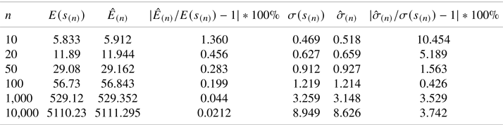
In Table 1, we compare  $E(s_{(n)})$ with
  $\hat {E}_{(n)}$ and
  $\sigma (s_{(n)})$ with
  $\hat {\sigma }_{(n)}$ in this manner: We fix
  $p=2/3$ and for
  $n=10$, 20, 50, 100, 1,000, and 10,000 we evaluate
  $E(s_{(n)})$ and
  $\sigma (s_{(n)})$ using Monte-Carlo (MC) simulation. Values of
  $\hat {E}_{(n)}$ and
  $\hat {\sigma }_{(n)}$ obtained based on Corollary 2.1.
Table 1. The number of Monte-Carlo repetitions is 100,000 for  $n=10, 20, 50, 100; 10,000$ for
  $n=1{,}000$; and 500 for
  $n=10{,}000$.

2.2. Second and third largest scores
Result 2.2 For  $j=1,\ldots ,n-1$,
 $$\lim_{n\rightarrow \infty}P(s^{*}_{(n-j)}< a_{n}+b_{n}t)=G(t)(1+e^{{-}t}+\cdots+e^{{-}jt}/j!),$$
where  $a_n$ and
  $b_n$ are defined in (1).
Proof. Follows from combining the multivariate central limit theorem with Theorems 4.5.2. and 5.3.4. in Leadbetter et al. [Reference Leadbetter, Lindgren and Rootzén9].
Corollary 2.2
 \begin{align} & E(s^{*}_{(n-1)})\sim \gamma b_n+a_n-b_n,\quad \sigma(s^{*}_{(n-1)})\sim \sqrt{\left(\frac{\pi^{2}}{6}-1\right)}\,b_n, \end{align}
 \begin{align} & E(s^{*}_{(n-2)})\sim \gamma b_n+a_n-3/2b_n,\quad \sigma(s^{*}_{(n-2)})\sim \sqrt{\left(\frac{\pi^{2}}{6}-1.25\right)}\, b_n \end{align}
Proof. Combing (2) with Theorem 2.2.2 in Leadbetter et al. [Reference Leadbetter, Lindgren and Rootzén9], we obtain the following result: if  $Y_1,\ldots ,Y_n$ are independent
  $\exp (1)$ random variables, then for
  $j=1,\ldots ,n-1$
 \begin{equation} {\lim_{n\rightarrow\infty}P(Y_{(n-j)}-\log(n)\leq t)=G(t)(1+e^{{-}t}+\cdots+e^{{-}jt}/j!)}. \end{equation}
The rest of the proof is similar to the proof of Corollary 2.1.
Substituting  $s^{*}_{(j)}=(s_{(j)}-E_n)/\sigma _n$ for
  $j=n-1, n-2$, we obtain the values
  $E(s_{(j)}), \sigma (s_{(j)}), \widehat {E}_{(j)}, \widehat {\sigma }_{(j)}$, which are similar to the corresponding values obtained in Corollary 2.1 for the case
  $j=n$.
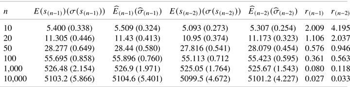
In the case where  $p=2/3$, we provide (in Table 2) numerical comparisons for the second and third largest scores in a similar manner as was done in Table 1.
Table 2. The number of Monte-Carlo repetitions is 100,000 for  $n=10, 20, 50, 100; 10,000$ for
  $n=1{,}000$; and 500 for
  $n=10{,}000$;
  $r_j=|\widehat {E}_{(j)}/E(s_{(j)})-1|*100\%$,
  $j=n-1, n-2$.
Acknowledgments
The author thank Abram Kagan for describing a score issue in chess round-robin tournaments with draws. The author also thank the Editor and anonymous referee for the comments.
Funding
This research was supported by grant no. 2020063 from the United States – Israel Binational Science Foundation (BSF), Jerusalem, Israel.
Conflict of interest
The authors declare no conflict of interest.