


1. Introduction
Thin liquid films flowing down a vertical fibre subject to thermal effects have been previously studied owing to their importance in a variety of industrial applications, which include dry cooling systems (Zeng et al. Reference Zeng, Sadeghpour, Warrier and Ju2017; Zeng, Sadeghpour & Ju Reference Zeng, Sadeghpour and Ju2018), and heat and mass exchangers for vapour, CO $_{2}$ and particle capture (Sadeghpour et al. Reference Sadeghpour, Zeng, Ji, Ebrahimi, Bertozzi and Ju2019, Reference Sadeghpour, Oroumiyeh, Zhu, Ko, Ji, Bertozzi and Ju2021; Zeng, Sadeghpour & Ju Reference Zeng, Sadeghpour and Ju2019). In addition to gravity and bulk surface tension, changes in liquid properties like surface tension and viscosity, which arise from the presence of a temperature gradient, influence the characteristics of these thin film flows. An improved understanding of the thermally-driven bead coalescence is crucial for the systematic design of these systems (Zeng et al. Reference Zeng, Sadeghpour and Ju2018).
Several research groups have experimentally investigated and analysed different flow regimes of liquid films flowing down a string (Kliakhandler, Davis & Bankoff Reference Kliakhandler, Davis and Bankoff2001; Duprat et al. Reference Duprat, Ruyer-Quil, Kalliadasis and Giorgiutti-Dauphiné2007; Ruyer-Quil & Kalliadasis Reference Ruyer-Quil and Kalliadasis2012; Ji et al. Reference Ji, Falcon, Sadeghpour, Zeng, Ju and Bertozzi2019). Kliakhandler et al. (Reference Kliakhandler, Davis and Bankoff2001) ran a set of experiments using a fibre with a size that is comparable to the liquid film thickness to study the effect of the flow rate on the flow regime. They qualitatively observed three different regimes of the interfacial patterns in the form of the travelling liquid beads. At low flow rates, the isolated droplet regime occurs where widely spaced large droplets flow down the fibre separated by secondary small-amplitude wavy patterns. At higher flow rates, the Rayleigh–Plateau (RP) flow regime emerges where a stable train of droplets propagate at a constant speed. If the flow rate is increased further, the convective instability regime emerges as collisions of large droplets occur in an irregular fashion. This instability can also be triggered by applying a gradient to the physical properties (i.e. surface tension/viscosity) of the liquid film along the fibre (Liu, Ding & Chen Reference Liu, Ding and Chen2018).
Prior experimental works have shown that maintaining a stable train of liquid beads is important for the reliable heat and mass transfer performance in many applications (Hattori, Ishikawa & Mori Reference Hattori, Ishikawa and Mori1994; Chinju, Uchiyama & Mori Reference Chinju, Uchiyama and Mori2000; Migita, Soga & Mori Reference Migita, Soga and Mori2005). For example, Nozaki, Kaji & Mod (Reference Nozaki, Kaji and Mod1998) investigated the cooling of thin films of a heated silicone oil flowing down a string. They demonstrated that at the same liquid flow rate, the string-of-beads flow exhibits a higher overall heat transfer coefficient than the annular film flow.
In our earlier work (Zeng et al. Reference Zeng, Sadeghpour, Warrier and Ju2017), we experimentally studied the relationship between flow characteristics and the overall effectiveness of heat exchange for thin liquid films flowing along a single string against a counterflowing air stream. The experiments showed that for very high liquid inlet temperatures, the flow no longer remains in the desired RP regime and can undergo a regime transition along the fibre. After travelling a certain distance away from the nozzle, the liquid droplets collide with each other, which causes cascade coalescence further downstream. This type of thermally-driven coalescence will be the focus of the present study.
For low flow rates where the inertial effects are negligible, the classical lubrication theory may be applied to model the dynamics of viscous films flowing down vertical cylinders. Under the small-interface-slope assumption, weakly nonlinear lubrication equations for the film thickness have been acquired in the works of Frenkel (Reference Frenkel1992), Chang & Demekhin (Reference Chang and Demekhin1999) and Kalliadasis & Chang (Reference Kalliadasis and Chang1994). Both stabilizing and destabilizing effects of the surface tension are incorporated into the model, which characterizes the axial and azimuthal curvatures of the free interface. In the work of Craster & Matar (Reference Craster and Matar2006), an asymptotic model was derived using a low Bond number, surface-tension-dominated theory. Full curvature terms were introduced in the work of Kliakhandler et al. (Reference Kliakhandler, Davis and Bankoff2001), and the existence of non-negative solutions to their model is shown in Ji, Taranets & Chugunova (Reference Ji, Taranets and Chugunova2020b). Recently, Ji et al. (Reference Ji, Falcon, Sadeghpour, Zeng, Ju and Bertozzi2019) investigated a full lubrication model that incorporates fully nonlinear curvature terms, slip boundary conditions and a film stabilization mechanism.
For higher flow rates where inertial effects are no longer negligible, Trifonov (Reference Trifonov1992), Ruyer-Quil et al. (Reference Ruyer-Quil, Treveleyan, Giorgiutti-Dauphiné, Duprat and Kalliadasis2008) and Duprat, Ruyer-Quil & Giorgiutti-Dauphiné (Reference Duprat, Ruyer-Quil and Giorgiutti-Dauphiné2009) investigated systems of coupled equations for the film thickness and the flow rate based on the integral boundary layer approach. This approach was further extended by Ji et al. (Reference Ji, Sadeghpour, Ju and Bertozzi2020a) through introduction of the film stabilization mechanism to address the influence of nozzle geometry on the downstream droplet dynamics.
Although many previous studies have focused on the dynamics of viscous thin films flowing down fibres, the thermal effects on the fibre coating dynamics have received less attention. For non-isothermal liquid films flowing along an inclined substrate, Kabova, Kuznetsov & Kabov (Reference Kabova, Kuznetsov and Kabov2012) derived a thin film equation that incorporates the influence of temperature-dependent viscosity and surface tension. This problem was also investigated by Ruyer-Quil et al. (Reference Ruyer-Quil, Scheid, Kalliadasis, Velarde and Zeytounian2005) using a weighted residuals approach. Haimovich & Oron (Reference Haimovich and Oron2011) studied the dynamics of a non-isothermal liquid film on an axially oscillating horizontal cylinder. More recently, Liu, Ding & Zhu (Reference Liu, Ding and Zhu2017), Liu et al. (Reference Liu, Ding and Chen2018), Ding & Wong (Reference Ding and Wong2017) and Ding et al. (Reference Ding, Liu, Wong and Yang2018) used lubrication models to study the influence of thermocapillarity on the coating flow down a vertical fibre subject to a temperature gradient. Their work focused on the Marangoni effects that originate from the linear dependence of the variation of surface tension with temperature. The works of Liu, Chen & Wang (Reference Liu, Chen and Wang2019) and Dong, Li & Liu (Reference Dong, Li and Liu2020) extended this result by considering a self-rewetting fluid (Batson, Agnon & Oron Reference Batson, Agnon and Oron2017) with the surface tension modelled as a quadratic function of temperature. Ding et al. (Reference Ding, Liu, Liu and Yang2019) also investigated the influence of thermally induced Marangoni effects and van der Waals attractions on the break-up of ultra-thin liquid films (Ji & Witelski Reference Ji and Witelski2017).
In this paper, we experimentally and theoretically investigate the thermal effects on the dynamics of thin viscous films flowing down a vertical fibre. We propose a lubrication model that incorporates both temperature-dependent viscosity and surface tension. Using this model, we numerically explore the downstream flow dynamics that form bead coalescence and obtain a good agreement with experimental results. A simplified ordinary differential equation (ODE) model is also developed to capture the influence of thermal effects on liquid bead dynamics.
The rest of this paper is organized as follows. In § 2, we describe the experimental set-up. In § 3, we derive the lubrication model for the film thickness by accounting for the presence of a temperature field. Section 4 provides a discussion on the stability of the model for both isothermal and weakly non-isothermal cases. In § 5.1, we present a numerical study of thermally-driven bead coalescence. This is followed by a comparison between the theory and experimental observations in § 5.2 and a brief investigation of a reduced ODE model in § 5.3. We present our concluding remarks in § 6. The appendix includes further details of full Navier–Stokes simulations.
2. Experiments
Figure 1(a) shows a schematic of the experimental set-up used in this study to investigate the characteristics of a liquid film flowing down a vertical string under a streamwise temperature gradient. The main parts of this set-up are: (1) a programmable syringe pump to pump the liquid through the nozzle at a fixed flow rate, (2) an in-line heater that controls the liquid temperature to a prescribed value at the nozzle inlet, (3) a stainless steel nozzle with an inner diameter of 1.2 mm and outer diameter of 1.55 mm, (4) a thermocouple to record the liquid temperature at the tip of the nozzle outlet (additional thermocouples are used to measure the axial temperature distribution of the liquid along the fibre), (5) a high-speed camera (frame rate of  $1000\ \textrm {frames}\,\textrm {s}^{-1}$) mounted on a translation stage, (6) a weight connected to the fibre to ensure the fibre stays vertical, (7) a liquid reservoir, (8) a weight scale to measure the liquid mass flow rate and (9) a computer for data acquisition.

Figure 1. (a) Schematic of the experimental set-up. An inline heater is integrated into the inlet of the nozzle to create a temperature gradient along the fibre. (b) Schematic of a thin liquid film flowing down a vertical cylindrical fibre under a streamwise temperature gradient.
The experiments were performed using polymer-based fibres with a diameter of 0.61 mm. The liquid mass flow rate was varied in the range of  $0.0013\text {--}0.016\ \textrm {g}\,\textrm {s}^{-1}$. The nozzle outer diameter was
  $\textrm {OD} = 1.55\ \textrm {mm}$. We used Rhodorsil silicone oils (v20, v50 and v100) as well-wetting liquids with a low surface energy. The inlet temperature of the liquid was changed in the range of
  $30\text {--}70\,^\circ \textrm {C}$. A summary of the experimental conditions is presented in table 1.
Table 1. Experimental cases of different Rhodorsil silicone oils (v20, v50 and v100), inlet temperatures, mass flow rates and liquid properties at  $20\,^\circ \textrm {C}$.

3. Model formulation
We consider a two-dimensional axisymmetric Newtonian fluid of density  $\rho$ flowing down a vertical cylinder of radius
  $R^*$ under a temperature gradient (see figure 1b). The dynamics of the flow is governed by gravity, bulk surface tension and temperature-dependent liquid properties. In this section, we first discuss the temperature distribution in the liquid film along the fibre and the temperature-dependent liquid properties. Then we will present a lubrication model that characterizes the thermal effects on the flow dynamics.
3.1. Temperature distribution along the fibre
Previous studies (Liu et al. Reference Liu, Ding and Chen2018) of the thermal effects on liquid films have typically assumed a constant temperature gradient. In this work, we instead represent the streamwise temperature variations under our experimental conditions using a solution to a lumped capacitance model
 \begin{equation} \varTheta = \exp \left[ - \left(\frac{{h}_{b} A_s}{m_b v_b c}\right) x^*\right]. \end{equation}
The works of Hattori et al. (Reference Hattori, Ishikawa and Mori1994) and Zeng et al. (Reference Zeng, Sadeghpour, Warrier and Ju2017) showed that the radial temperature variation within each liquid bead is negligible owing to efficient mixing associated with internal circulation within the bead. Axial heat conduction is neglected. In the model (3.1),  $\varTheta = {(T^*-T_0^*)}/{\varDelta T}$ is the dimensionless temperature, where
  $\varDelta T = T^*_{{IN}} - T^*_0$ is the temperature scale set by the difference between the inlet temperature
  $T^*_{{IN}}$ and the room temperature
  $T^*_0$. Here
  $A_s$ represents the surface area of the liquid beads,
  $c$ is the specific heat of the liquid,
  $v_{b}$ is the liquid bead velocity,
  $m_b$ is the mass of each bead,
  $x^*$ is the distance from the inlet and
  ${h}_{b}$ is the liquid bead-to-air heat transfer coefficient. We use the empirical relationship for the heat transfer coefficient of flow around a sphere (Whitaker Reference Whitaker1972; Mills Reference Mills1995) to obtain the value of
  ${h}_{b}$,
 \begin{equation} \frac{{h}_{b}D_{b}}{k_{air}} = 2 + (0.4 Re_{b}^{1/2} + 0.06 Re_{b} ^ {2/3}) Pr_{air}^{0.4}. \end{equation}
Here,  $Re_{b} = \rho _{air} v_{b} D_{b}/\mu _{air}$ is the bead Reynolds number,
  $D_{b}$ is the bead diameter and
  $Pr_{air}$ is the Prandtl number of air. In addition,
  $\mu _{air}$,
  $\rho _{air}$ and
  $k_{air}$ are the viscosity, density and thermal conductivity of air, respectively. The temperature profiles obtained from the lumped capacitance model (3.1) are used later in the lubrication model to represent the axial variations in the surface tension and viscosity along the fibre.
As shown in figure 2, the model captures the experimentally measured liquid temperature profiles well. For later convenience, we rewrite the dimensionless temperature distribution in a rescaled form
 \begin{equation} \varTheta_I(x) = 1 - \frac{1-\exp(-\chi x)}{1-\exp(-\chi L_0)}, \end{equation}
where  $x$ is the dimensionless streamwise spatial variable and
  $L_0$ is the dimensionless downstream position where the room temperature
  $T_0^*$ is nominally reached. The temperature profile (3.3) satisfies
  $\varTheta _I(0) = 1$ and
  $\varTheta _I(L_0) = 0$, and the dimensionless parameter
  $\chi$ specifies the temperature gradient. In all simulations, we set
  $L_0 = L_0^*/\mathcal {L}$, where
  $L_0^* = 0.5\ \textrm {m}$ and
  $\mathcal {L}$ is the length scale in the streamwise direction, which will be defined in § 3.3.

Figure 2. Temperature profiles measured in experiments along the fibre for silicone oil v50 with different inlet temperatures compared with the prediction based on the model (3.1). The parameters are  $h_b = 44\ \textrm {W}\,(\textrm {m}^{2}\,\textrm {K})^{-1}$,
  $A_s =13.2\ \textrm {mm}^2$,
  $c = 1510\ \textrm {J}\,(\textrm {kg}\,\textrm {K})^{-1}$,
  $m_b=2.04\times 10^{-6}\ \textrm {kg}$ and
  $v_b=19.2\ \textrm {mm}\,\textrm {s}^{-1}$.
3.2. Temperature-dependent liquid properties
Liquid properties can change significantly as the temperature is varied. In this work, we focus on the influence of temperature on the surface tension and viscosity of the liquid.
To characterize the temperature dependence of the surface tension of our liquid, we measured the rising height,  $h_{{rise}}$, in a capillary tube with an inner diameter,
  $r_{{tube}}$, of 0.5 mm at various temperatures (
 $20\text {--}110\,^\circ \textrm {C}$). We then used
  $\sigma = ({ r_{{tube}} h_{{rise}} \rho g})/({2 \cos \theta })$ to estimate the surface tension at each temperature (Washburn Reference Washburn1921). Here,
  $\theta$ is the contact angle on the capillary tube wall that we measured independently. All the experiments were performed in an isothermal container.
Figure 3(a) shows the experimental results for the surface tension,  $\sigma$ (
 $\textrm {mN}\,\textrm {m}^{-1}$), of silicone oil v50. The experimental uncertainty in the measured surface tension is estimated to be
  $0.3\ \textrm {mN}\,\textrm {m}^{-1}$ and the uncertainty in the measured temperatures is estimated to be
  ${\pm }0.5\,^\circ \textrm {C}$.

Figure 3. (a) Surface tension and (b) viscosity of silicone oil v50 as functions of temperature  $T^*$.
The kinematic viscosity  $\nu (T^*)\ (\text {mm}^2\,\text {s}^{-1})$ of silicone oil v50 as a function of the temperature
  $T^*\ (^\circ \textrm {C})$ was provided by the manufacturer (see Shin-etsu 2005). A plot of the relation between viscosity and temperature is included in figure 3(b).
For simplicity, in the model derived here, we make an approximation that the kinematic viscosity  $\nu$ and the surface tension
  $\sigma$ of the liquid are linearly dependent on temperature,
 \begin{equation} \nu(T^*) = \nu_0 - \nu_T (T^*-T_0^*) ,\quad \sigma(T^*) = \sigma_0 - \sigma_T (T^*-T_0^*) , \end{equation}
where  $\nu _0,\nu _T,\sigma _0, \sigma _T > 0$ are constants. Using the dimensionless temperature variable, one can also write
  $\nu = \nu _0 - \nu _T \varDelta T\varTheta$ and
  $\sigma = \sigma _0 - \sigma _T \varDelta T \varTheta .$
In this paper, we have the reference room temperature  $T_0^*=20\,^\circ \textrm {C}$,
  $\sigma _T = 0.0504\ \textrm {mN}\,(\textrm {m}\,^{\circ }\textrm {C})^{-1}$ and
  $\nu _T = (\nu _0-\nu (T^*_{{IN}}))/\varDelta T$. The density of the liquid is assumed to be constant.
3.3. Lubrication model
Next we derive the governing equations following the works of Craster & Matar (Reference Craster and Matar2006), Ruyer-Quil et al. (Reference Ruyer-Quil, Treveleyan, Giorgiutti-Dauphiné, Duprat and Kalliadasis2008) and Ji et al. (Reference Ji, Falcon, Sadeghpour, Zeng, Ju and Bertozzi2019). We choose the length scale in the radial direction  $y$ as
  $\mathcal {H}$ and the length scale in the streamwise direction
  $x$ as
  $\mathcal {L} = \mathcal {H}/\epsilon$. The scale ratio
  $\epsilon$ is set by the balance between the surface tension and the gravity
  $g$, and is given by
  $\epsilon = (\rho g \mathcal {H}^2/\sigma _0)^{1/3}$. This scale ratio is small (approximately
  $0.35$) in typical experiments and can also be rewritten as
  $\epsilon = We^{-1/3}$, where the Weber number
  $We = (l_c/\mathcal {H})^2$ compares the capillary length
  $l_c = \sqrt {\sigma _0/(\rho g)}$ with the radial length scale
  $\mathcal {H}$. The characteristic streamwise velocity is
  $\mathcal {U}=(g\mathcal {H}^2)/{\nu _0}$, and the pressure and time scales are given by
  $\rho g \mathcal {L}$ and
  $(\nu _0\mathcal {L})/(g\mathcal {H}^2)$, respectively.
Following the approach in Ji et al. (Reference Ji, Falcon, Sadeghpour, Zeng, Ju and Bertozzi2019, Reference Ji, Sadeghpour, Ju and Bertozzi2020a), we include a film stabilization term  $\varPi (h)$,
 \begin{equation} \varPi(h) ={-}\frac{A}{h^3}, \end{equation}
where  $A>0$ is a stabilization parameter. This term takes the functional form of the long-range disjoining pressure of the van der Waals model that characterizes the microscopic quantities for wetting liquids, and
  $A$ is typically referred as a Hamaker constant (de Gennes Reference de Gennes1985).
The dynamics of the axisymmetric flows is governed by the Navier–Stokes equations, the continuity equation and the energy equation. This system is coupled with the temperature-dependent viscosity and surface tension given by (3.4a,b). With these scales, we write the non-dimensional Navier–Stokes equations using dimensionless variables as
 \begin{gather} \epsilon^2Re\left(u_{t} + u u_{x} + vu_{y}\right) ={-}p_{x}-\varPi_x+1+(1-\kappa\varTheta)\left(\frac{u_{y}}{y}+u_{yy}+\epsilon^2 u_{xx}\right), \end{gather}
 \begin{gather} \epsilon^4Re\left( v_{t} + v v_{y} + uv_{x}\right) ={-}p_{y}+\epsilon^2(1-\kappa\varTheta)\left(\frac{v_{y}}{y} +v_{yy}-\frac{v}{y^{2}}+\epsilon^2 v_{xx}\right), \end{gather}
 \begin{gather} v_{y}+\frac{v}{y} + u_{x} = 0, \end{gather}
where the Reynolds number  $Re = \mathcal {UL}/\nu _0$, and the constants
  $\kappa = {\nu _T\varDelta T}/{\nu _0}$ and
  $\omega = {\sigma _T\varDelta T}/{\sigma _0}$ scale the relative change in viscosity and surface tension as the temperature is varied. The balances of normal and tangential stresses at
  $y = h+R$ are expressed as
 \begin{gather} (1-\epsilon^2 h_x^2)(\epsilon^2 v_x+u_y) + 2\epsilon^2 h_x(v_y-u_x) ={-}Ma \frac{(1+\epsilon^2 h_x^2)^{1/2}}{1-\kappa\varTheta}(h_x\varTheta_y + \varTheta_x), \end{gather}
 \begin{gather} p+\varPi = \left(\frac{\alpha}{\epsilon^2(1+\alpha h)(1+\epsilon^2 h_x^2)^{1/2}} - \frac{h_{xx}}{(1+\epsilon^2 h_x^2)^{3/2}}-\frac{A}{h^3}\right)(1-\omega \varTheta)\nonumber\\ +\frac{2\epsilon^2(1-\kappa\varTheta)}{1+\epsilon^2 h_x^2}\left[\epsilon^2(h_x^2 u_x - h_x v_x)-h_x u_y + v_y\right], \end{gather}
where  $Ma = (\sigma _T \varDelta T)/(\rho g \mathcal {H} \mathcal {L})$ is the Marangoni parameter,
  $\alpha = \mathcal {H}/R^*$ is the aspect ratio of the characteristic radial length scale and the fibre radius, and the dimensionless fibre radius is
  $R = R^*/\mathcal {H}$. At the interface between the solid substrate and the liquid,
  $y = R$, we impose the no slip and no penetration boundary conditions,
 \begin{equation} v = u = 0, \quad \text{at} \ y = R. \end{equation}
The kinematic boundary condition at  $y = R+h$ is given by
 \begin{equation} h_t + u h_{x} = v, \quad \text{at} \ y = R+h. \end{equation}
 Next, we simplify the above set of governing equations following Ruyer-Quil et al. (Reference Ruyer-Quil, Treveleyan, Giorgiutti-Dauphiné, Duprat and Kalliadasis2008). Under the lubrication approximation, we neglect the inertial contributions by assuming that  $Re = O(1)$ and
  $\epsilon \ll 1$. Omitting the terms of order
  $O(\epsilon ^2)$, we rewrite the leading order non-dimensional reduced momentum and continuity equations for the velocity field
  $(u,v)$ and the dynamic pressure
  $p$ as
 \begin{gather} 1 -\frac{\partial p}{\partial x}-\frac{\partial \varPi}{\partial x}+(1-\kappa\varTheta)\left(\frac{\partial^2 u}{\partial y^2} +\frac{u_y}{y}\right)= 0, \end{gather}
 \begin{gather} {-}\frac{\partial p}{\partial y} = 0, \end{gather}
 \begin{gather}\frac{\partial u}{\partial x}+\frac{\partial v}{\partial y} +\frac{v}{y} = 0. \end{gather}
Based on our discussion in § 3.1, the radial temperature variations within liquid droplets and across the inter-bead precursor layer are negligible compared with the streamwise temperature variations. Therefore, we assume that the temperature is constant in the radial direction and only varies in the axial direction in the leading order,  $\varTheta = \varTheta _I(x)$. The balance of tangential stresses at the free surface
  $y = h + R$ reduces to
 \begin{equation} u_y ={-}\frac{Ma}{1-\kappa\varTheta}(h_x\varTheta_y + \varTheta_x) ={-}\frac{Ma\varTheta_x}{1-\kappa\varTheta}. \end{equation}
The balance of normal stresses at the free surface  $y = h + R$ becomes
 \begin{equation} p+\varPi = \left(\frac{\alpha}{\epsilon^2(1+\alpha h)}-\frac{\partial^2 h}{\partial x^2}-\frac{A}{h^3}\right) (1-\omega\varTheta). \end{equation}
The two terms on the right-hand side of (3.7e),  $\alpha /(\epsilon ^2(1+\alpha h))$ and
  $\partial ^2 h/\partial x^2$, describe both the destabilizing and stabilizing roles of the surface tension that originate from the azimuthal and axial curvature of the free surface, respectively. The balance between the azimuthal and axial scales is characterized by
  $\alpha$ and
  $\epsilon$. Here we use linear forms for both curvature terms; a discussion of other appropriate forms for the curvature terms can be found in Ji et al. (Reference Ji, Falcon, Sadeghpour, Zeng, Ju and Bertozzi2019).
Combining the kinematic boundary condition (3.6g), the no slip and no penetration boundary conditions (3.6f) and the continuity equation (3.7c) lead to the mass conservation equation
 \begin{equation} (1+\alpha h)\frac{\partial h}{\partial t} + \frac{\partial q}{\partial x} = 0, \quad \text{where } q = \frac{1}{R}\int_{R}^{h+R} uy\,{\textrm{d}y}. \end{equation}
Equation (3.7b) indicates that the pressure  $p$ is a function of
  $x$ only. Integrating (3.7a) twice and using (3.7d) yields
 \begin{gather} u =\frac{1}{1-\kappa\varTheta(x)}\left[\frac{1-p_x-\varPi_x}{2}\left( -\frac{1}{2}(y^2-R^{2})+(h+R)^2\ln\left(\frac{y}{R}\right)\right)\right.\nonumber\\ \left. - Ma\varTheta_x (R+h)\ln\left(\frac{y}{R}\right)\vphantom{\frac{1-p_x-\varPi_x}{2}}\right]. \end{gather}
Because  $\alpha = \mathcal {H}/R^* = 1/R$, by using (3.8), we obtain the form of flux
  $q$
$q$
 \begin{equation} q = \frac{1}{1-\kappa\varTheta}\left(\frac{h^3}{3}\phi(\alpha h)(1-p_x-\varPi_x)-\frac{1}{2}Ma\varTheta_x h^2\psi(\alpha h)\right), \end{equation}
where the shape factors  $\phi$ and
  $\psi$ are functions defined by
 \begin{gather} \phi(X) = \frac{3}{16X^3}[(1+X)^4(4\ln(1+X)-3)+4(1+X)^2-1], \end{gather}
 \begin{gather} \psi(X) = \frac{1+X}{X^2}\left[(1+X)^2\ln(1+X)-X\left({\frac{1}{2}} X + 1\right)\right]. \end{gather}
In the limit of  $X \to 0$, we have
 \begin{equation} \phi(X) = 1+X+\tfrac{3}{20}X^2+O(X^3),\quad \psi(X)=1+\tfrac{4}{3}X+\tfrac{1}{4}X^2+O(X^3). \end{equation}
Given a dimensional volumetric flow rate  $Q_m$ and fibre radius
  $R^*$, we define the volumetric flow rate per circumference unit
  $q_0^*$ as
  $q_0^* = Q_m/(2{\rm \pi} \rho R^*)$. We set the characteristic axial length scale
  $\mathcal {H}$ by solving (3.10) for
  $h$ with
  $q = q_0^*$,
  $\varTheta \equiv 0$,
  $\varPi_x\equiv 0$ and
  $p_x\equiv 0$. That is, we set the length scale
  $\mathcal {H}$ by the film thickness
  $h_N^*$ of a uniform Nusselt flow at room temperature
  $T_0^*$ with constant dynamic viscosity
  $\nu _0$ (Ruyer-Quil et al. Reference Ruyer-Quil, Treveleyan, Giorgiutti-Dauphiné, Duprat and Kalliadasis2008; Duprat et al. Reference Duprat, Ruyer-Quil and Giorgiutti-Dauphiné2009).
Finally, by rescaling the time scale  $t \to {t}/{\phi (\alpha )}$, and combining (3.8), (3.10) and (3.7e), we obtain the dimensionless governing equation for
  $0 \le x \le L$,
 \begin{equation} \frac{\partial}{\partial t} \left(h+\frac{\alpha}{2}h^2\right) + \frac{\partial q}{\partial x} = 0, \end{equation}
where the flux takes the form
 \begin{equation} q = \mathcal{M}(h)\left(1-\frac{\partial }{\partial x}\left[(1-\omega\varTheta)\left(\mathcal{Z}(h)-h_{xx}\right)\right]\right) -\frac{h^2}{2}\frac{\varTheta_xMa}{1-\kappa\varTheta} \frac{\psi(\alpha h)}{\phi(\alpha)}, \end{equation}
where the mobility function is
 \begin{equation} \mathcal{M}(h) = \frac{h^3}{3(1-\kappa\varTheta)}\frac{\phi(\alpha h)}{\phi(\alpha)}, \end{equation}
and the function  $\mathcal {Z}(h)$ consists of the destabilizing azimuthal curvature term
  $\alpha /(\eta (1+\alpha h))$ and the film stabilization term
  $\varPi (h)$,
 \begin{equation} \mathcal{Z}(h) = \frac{\alpha}{\eta (1+\alpha h)} + \varPi(h), \quad \varPi(h) ={-}\frac{A}{h^3}, \end{equation}
where the scaling parameter  $\eta = \epsilon ^2$.
This choice of time scale leads to a normalized mobility function that satisfies  $\mathcal {M} = 1/3$ for
  $h = 1$ and
  $\varTheta \equiv 0$. The model (3.14) can be written as a fourth-order nonlinear partial differential equation (PDE) for the thickness
  $h(x,t)$. It accounts for temperature-dependent viscosity and surface tension gradients, gravity and azimuthal instabilities, but neglects the inertia and streamwise viscous dissipation that are included in the work of Ruyer-Quil et al. (Reference Ruyer-Quil, Trevelyan, Giorgiutti-Dauphiné, Duprat and Kalliadasis2009). We note that because
  $0 \le \kappa < 1$ and
  $0\le \varTheta \le 1$, we have
  $0<1-\kappa \varTheta \le 1$ in (3.14b) and (3.14c).
Compared with the prior work in Liu et al. (Reference Liu, Ding and Chen2018) that focuses on the thermocapillarity effects in similar dynamics, this new model includes additional physics through the temperature-dependent viscosity and does not require the aspect ratio  $\alpha$ to satisfy
  $\alpha \ll 1$. Our model with
  $\kappa = Ma = \omega=A = 0$ is also consistent with the model derived in the work of Craster & Matar (Reference Craster and Matar2006) except for a scaling difference.
In the limit  $\alpha \to 0$, the model (3.14) describes the dynamics of a draining film flowing down an incline under thermal effects. If we assume that the viscosity is constant and set
  $\kappa=Ma=\omega=A = 0$, (3.14) reduces to (3.15), which describes thin film dynamics driven by the gravity and a surface tension gradient owing to a temperature gradient,
 \begin{equation} h_t + ({\tfrac{1}{3}}h^3-{\tfrac{1}{2}}h^2\varTheta_xMa)_x={-}{\tfrac{1}{3}}(h^3 h_{xxx})_x. \end{equation}
The cubic term and quadratic term on the left-hand side of (3.15) originate from gravity and the Marangoni stress, respectively. In this paper, we consider a decreasing temperature field,  $\varTheta _x < 0$, and the surface tension gradient is expected to promote the downward movement of the film.
4. Stability analysis
In this section, we investigate the instability of the model by considering two cases, (a) the isothermal case where the fibre is uniformly heated and (b) the weakly non-isothermal case, where a temperature gradient is imposed along the fibre. We will discuss the influence of the temperature-dependent liquid properties on both the temporal instability and absolute/convective instability transition of the system.
4.1. Isothermal films
We begin by considering the flow instability of a uniformly heated thin fluid film flowing down a vertical fibre. Specifically, we study an isothermal film with spatially-constant surface tension and viscosity at a temperature  $\varTheta (x) \equiv \varTheta _0$ and
  $\textrm {d}\varTheta /{\textrm {d}x} = 0$, where
  $0 \le \varTheta _0 \le 1$. Then the governing equation (3.14) reduces to
 \begin{align} \frac{\partial}{\partial t} \left(h+\frac{\alpha}{2}h^2\right) + \frac{\partial}{\partial x}\left[\mathcal{M}(h)\left(1-(1-\omega\varTheta_0)\frac{\partial }{\partial x}\left(\frac{\alpha}{\eta (1+\alpha h)}-h_{xx} + \varPi(h)\right)\right)\right] = 0, \end{align}
where the mobility function takes the form  $\mathcal {M}(h) = {[h^3\phi (\alpha h)]}/{[3(1-\kappa \varTheta _0)\phi (\alpha )]}.$ We perturb the uniform base state
  $\bar {h} = 1$ by an infinitesimal Fourier mode,
 \begin{equation} h = \bar{h} + \bar{\psi} \,\textrm{e}^{\mathrm{i}(k x - \varLambda t)}, \end{equation}
where  $k$ is the wavenumber,
  $\varLambda$ is the wave frequency and
  $\bar {\psi } (\ll 1)$ is the initial amplitude. Expanding the PDE (4.1) then gives the dispersion relation
 \begin{equation} \varLambda = C(\alpha,\kappa, \varTheta_0)k + \mathrm{i} k^2 D(\alpha,\kappa, w, \varTheta_0)\left[{-}k^2+\frac{\alpha^2}{\eta(1+\alpha)^2}-3A\right], \end{equation}
where
 \begin{align} C(\alpha,\kappa,\varTheta_0) = \frac{\alpha\phi'(\alpha)+3\phi(\alpha)}{3(1-\kappa\varTheta_0)(1+\alpha)\phi(\alpha)},\quad D(\alpha,\kappa, w, \varTheta_0) = \frac{1-\omega\varTheta_0}{3(1-\kappa\varTheta_0)(1+\alpha)}. \end{align}
 The relation (4.3) indicates that the azimuthal curvature term  $\alpha /(\eta (1+\alpha h))$ is destabilizing, and both the streamwise curvature term
  $h_{xx}$ and the film stabilization term
  $\varPi (h)$ are stabilizing. For
  $\kappa >0$, the temporal instability is enhanced by the thermal-viscosity influence.
Following the work of Ji et al. (Reference Ji, Falcon, Sadeghpour, Zeng, Ju and Bertozzi2019), we select the stabilization parameter  $A$ based on the dimensional thickness
  $\epsilon _p = \mathcal {H}h_c$ of a stable uniform layer based on experiments, where
  $h_c$ is the dimensionless thickness of the stable coating film. Specifically, we pick
  $A = A_c$, where
 \begin{equation} A_c = \frac{\alpha^2 h_c^4}{3\eta(1+\alpha h_c)^2}, \end{equation}
which ensures that any thin flat film  $h\le h_c$ is linearly stable (
 $\text {Im}(\varLambda ) < 0$) for all real wave numbers
  $k > 0$.
To understand the spatiotemporal stability of the uniform state, we consider the peak of a localized wave packet that travels with a speed given by the group velocity  $v_g = \textrm {d} \varLambda /\textrm {d} k$, where both
  $\varLambda$ and
  $k$ are complex. The merging of two disconnected spatial branches at a point in the complex
  $k$-plane leads to a vanishing group velocity,
  $v_g|_{k=k_0} = 0$, which defines the absolute wavenumber
  $k_0$ and the corresponding absolute frequency
  $\varLambda _0 = \varLambda (k_0)$ (Duprat et al. Reference Duprat, Ruyer-Quil, Kalliadasis and Giorgiutti-Dauphiné2007; Scheid, Kofman & Rohlfs Reference Scheid, Kofman and Rohlfs2016). For
  $\text {Im}(\varLambda _0) >0$, the system presents absolute instability; for
  $\text {Im}(\varLambda _0) <0$, the fluid film shows convective instability. The absolute/convective (A/C) instability transition corresponds to a real absolute frequency,
  $\text {Im}(\varLambda _0) = 0$.
Following the approach in the work of Duprat et al. (Reference Duprat, Ruyer-Quil, Kalliadasis and Giorgiutti-Dauphiné2007), we introduce the transformation
 \begin{equation} k = \tilde{k}\left(\frac{C}{3D}\right)^{1/3},\quad \varLambda = \tilde{\varLambda} C\left(\frac{C}{3D}\right)^{1/3}, \quad \frac{\alpha^2}{\eta(1+\alpha)^2}-3A = \beta\left(\frac{C}{3D}\right)^{2/3} \end{equation}
and reduce the dispersion relation (4.3) to the equation
 \begin{equation} \tilde{\varLambda} = \tilde{k} + \mathrm{i} \frac{\tilde{k}^2}{3}(\beta-\widetilde{k^2}). \end{equation}
This corresponds to the dispersion relation for a weakly nonlinear lubrication model studied in Frenkel (Reference Frenkel1992). Based on the calculation in Duprat et al. (Reference Duprat, Ruyer-Quil, Kalliadasis and Giorgiutti-Dauphiné2007), the instability of the system becomes absolute when  $\beta > \beta _{ca}\equiv [9/4(-17+7\sqrt {7})]^{1/3}\approx 1.507$. This leads to the A/C threshold for the instability of isothermal films,
 \begin{equation} \frac{3(1-\omega\varTheta_0)\phi(\alpha)}{\alpha\phi'(\alpha)+3\phi(\alpha)}\left(\frac{\alpha^2}{\eta(1+\alpha)^2}-3A\right)^{3/2}=\beta_{ca}^{3/2}, \end{equation}
which shows that the A/C marginal curve is influenced by the thermal effects only through the prefactor  $1-\omega \varTheta _0$, and the temperature-dependent viscosity does not play a role. We note that this conclusion may change if moderate inertia effects or streamwise heat diffusion is included in the model (Ruyer-Quil et al. Reference Ruyer-Quil, Treveleyan, Giorgiutti-Dauphiné, Duprat and Kalliadasis2008; Scheid et al. Reference Scheid, Kofman and Rohlfs2016; Ding et al. Reference Ding, Liu, Wong and Yang2018).
Following the studies of Duprat et al. (Reference Duprat, Ruyer-Quil and Giorgiutti-Dauphiné2009) and Ruyer-Quil & Kalliadasis (Reference Ruyer-Quil and Kalliadasis2012), we rewrite the threshold (4.8) in terms of  $R^*/l_c$ and
  $\alpha$ and obtain
 \begin{equation} \frac{1}{C_k(\alpha)(1+\alpha)^4}\left[\alpha^{2/3}-3(\alpha+1)^2\left(\frac{R^*}{l_c}\right)^{4/3}A\right]^{3/2} = \beta_{ca}^{3/2}\mathcal{S}^2, \end{equation}
where  $R^*/l_c$ is the ratio of the fibre radius
  $R^*$ and the capillary length
  $l_c$,
  $C_k(\alpha )$ is the linear wave speed
  $C(\alpha ,\kappa ,\varTheta _0)$ in (4.4a,b) for
  $\kappa \varTheta _0=0$, and
  $\mathcal {S}=({R^*}/{l_c})[1-\omega \varTheta _0]^{-1/2}$. For
  $\omega \varTheta _0 = 0$ and
  $A=0$, this threshold (4.9) is consistent with the A/C threshold proposed in the works of Ruyer-Quil & Kalliadasis (Reference Ruyer-Quil and Kalliadasis2012) and Duprat et al. (Reference Duprat, Ruyer-Quil and Giorgiutti-Dauphiné2009).
Figure 4 presents the A/C instability regimes predicted by (4.9) for isothermal films with  $A = 0$. Downstream flow dynamics for the experiments in table 1 are shown in figure 4 with circles representing the RP flow regime and crosses representing droplet coalescence dynamics. This analysis suggests that for all the experimental cases in the present study, the flow dynamics of the uniformly heated isothermal liquid film at the temperature
  $T^*_{{IN}}$ fall in the absolute instability regime. Therefore, the bead coalescence observed in our experiments cannot take place without the presence of a temperature gradient. In particular, for
  $\omega = 0$, we note that for a spatially-constant temperature field
  $\varTheta (x) \equiv \varTheta _0$, a direct transformation
  $t \to t(1-\kappa \varTheta )$ in (3.14) leads to a PDE without any temperature-dependent terms. Therefore, for any trains of travelling beads in the absolute RP regime, we expect the flow to stay in the RP regime when the temperature is uniformly elevated across the fibre. This indicates that the non-uniform temperature field
  $\varTheta (x)$ is crucial for the bead coalescence observed in our experiments.

Figure 4. The absolute and convective (A/C) instability regimes in the parameter plane of  $\alpha$ and
  $\mathcal {S}$ predicted by (4.9) with
  $\beta _{ca} = 1.507$ and
  $A = 0$. The circle symbols represent experiments that are in RP regime and the cross symbols represent experiments with downstream bead coalescence.
4.2. Weakly non-isothermal films
Next, we show that for the weakly non-isothermal case, where the fibre is non-uniformly heated, both temperature-dependent viscosity and surface tension play an important role in determining the instability of the film. For simplicity, we consider the temperature  $\varTheta =O(\delta )\ll 1$ that linearly decreases in space in the leading order,
 \begin{equation} \varTheta(x) = \delta\bar{\varTheta}(x) = \delta(1-\theta_1 x) + O(\delta^2) ,\quad \text{where }\theta_1 = 1/L \ll 1. \end{equation}
This temperature  $\varTheta (x)$ satisfies
  $\varTheta (0) \approx \delta$ and
  $\varTheta (L) \approx 0$. Substituting (4.10) into the governing equation (3.14), for
  $\delta \ll 1$, we obtain the expansion for flux
 \begin{equation} q =(1+\kappa\delta\bar{\varTheta})\left\{ M_0(h)\left(1-\frac{\partial }{\partial x}[(1-\omega\delta\bar{\varTheta})\left(\mathcal{Z}(h)-h_{xx}\right)]\right) +\delta\theta_1Ma M_1(h)\right\} + O(\delta^2), \end{equation}
where
 \begin{equation} M_0(h) = \frac{h^3 \phi(\alpha h)}{3\phi(\alpha)}, \quad M_1(h) = \frac{h^2}{2}\frac{\psi(\alpha h)}{\phi(\alpha)}. \end{equation}
For  $\delta \ll 1$, the uniform film
  $\bar {h} = 1$ is a quasi-steady state of the system. Similar to the isothermal case, we apply the perturbation (4.2) to the governing equation and obtain the relation
 \begin{equation} \varLambda = \varLambda_0(k) + \delta \varLambda_1(k,x) + O(\delta^2), \end{equation}
where the leading-order term is given by
 \begin{equation} \varLambda_0(k)=k\frac{\alpha\phi'(\alpha)+3\phi(\alpha)}{3(1+\alpha)\phi(\alpha)} + \mathrm{i} k^2 \frac{1}{3(1+\alpha)}\left[{-}k^2+\frac{\alpha^2}{\eta(1+\alpha)^2}-3A\right], \end{equation}
which is consistent with the dispersion relation (4.3) for the isothermal case for  $\kappa =\omega =0$. The
  $O(\delta )$ term
  $\varLambda _1$ depends on both the wavenumber
  $k$ and the spatial variable
  $x$,
$x$,
 \begin{align} \varLambda_1(k,x) &= {\frac{k}{3(\alpha+1)}}{ ( {k}^{2}+\mathcal{Z}'(1) ) [ \mathrm{i} ( -\kappa+\omega ) \bar{\varTheta}(x) k+\theta_1\, ( \kappa-2\,\omega ) ] } \nonumber\\ &\quad + {\frac{1}{\alpha+1}}[( -\theta_1\,\omega\, \mathcal{Z} ( 1 ) k+ ( \bar{\varTheta}(x) k+\mathrm{i}\theta_1 ) \kappa ) M_0'(1) +\text{Ma}\,\theta_1\,kM_1'(1) ]. \end{align}
This analysis reveals the combined effects of the temperature-dependent liquid properties on the film stability in the non-isothermal scenario through parameters  $\kappa$,
  $\omega$ and
  $Ma$.
$Ma$.
5. Results
5.1. Numerical simulations
We first perform numerical simulations of the PDE (3.14) to explore the influence of the thermal effects on the flow patterns. The dynamics near the nozzle are of interest because that is where the steepest temperature gradient occurs. To capture the near-nozzle dynamics, we set the initial conditions for the model (3.14) based on the nozzle geometry using a piece-wise linear profile for the film thickness  $h$,
$h$,
 \begin{equation} h(x, 0) = \begin{cases} 1, & x > x_L\\ h_{{IN}}+(1-h_{{IN}})x/x_L, & 0\le x \le x_L \end{cases}, \end{equation}
where  $h_{{IN}} = ({\tfrac {1}{2}}\text {OD}-R^*)/\mathcal {H}$ is determined by the difference between the nozzle outer diameter OD and the fibre radius
  $R^*$, and
  $x_L = 10$ is used for all simulations. We impose the following Dirichlet boundary conditions at the inlet
  $x = 0$ and the Neumann boundary conditions at the outlet
  $x = L$,
 \begin{equation} \left. \begin{gathered} h(0,t)=h_{{IN}}, \quad q(0,t)=1/3\quad \text{at } x = 0, \\ h_x(L,t) = 0, \quad h_{xx}(L,t) = 0 \quad \text{at } x = L. \end{gathered} \right\} \end{equation}
To numerically solve the model (3.14), we use a Keller-box-based centred finite difference method where the fourth-order differential equation is decomposed into a system of first-order differential equations:
 \begin{equation} \left. \begin{gathered} k = h_x,\quad p = {\frac{\alpha}{\eta (1+\alpha h)}}-k_x, \quad \left(h+\frac{\alpha}{2}{h^2}\right)_t + q_x = 0,\\ q = {\mathcal{M}(h)(1-[(1-\omega\varTheta)(p+\varPi(h))]_x)-\frac{h^2}{2}\frac{\varTheta_xMa}{1-\kappa\varTheta} \frac{\psi(\alpha h)}{\phi(\alpha)}}. \end{gathered} \right\} \end{equation}
 For most numerical simulations shown in this subsection, the boundary conditions (5.2) with  $h_{{IN}}=1.46$ is used, which corresponds to the dimensional nozzle diameter
  $\textrm {OD}=1.55\ \textrm {mm}$. Moreover, we set
  $\alpha = 1.054$ and
  $\eta = 0.132$, which correspond to the dimensional fibre radius
  $R^*=0.305\ \textrm {mm}$ and the flow rate
  $Q_m = 8\times 10^{-6}\ \textrm {kg}\,\textrm {s}^{-1}$ for silicone oil v50.
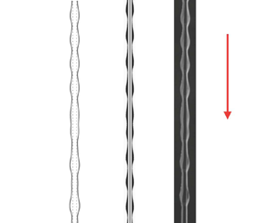
Starting from identical initial conditions (5.1), a comparison of the long-time dynamics of the model (3.14) with and without thermal effects is shown in figure 5. Figure 5(a) shows that without thermal effects ( $T^*_{{IN}} = T_0^*$), the downstream dynamics (
 $x^* > 60\ \textrm {mm}$) stabilizes into a sequence of equally-spaced travelling beads, which is a signature that the RP regime is attained. Figure 5(b) shows the response of the bead dynamics to the imposed temperature distribution
  $\varTheta = \varTheta _I$ in (3.3) with the inlet temperature
  $T^*_{{IN}} = 65\,^\circ \textrm {C}$ and
  $\chi =0.0085$. Close to the nozzle, the bead size and spacing are significantly smaller than those in figure 5(a), which shows droplet compression in the high-temperature region. In the downstream region of
  $80\ \text {mm} < x^* < 160\ \textrm {mm}$ in figure 5(b), where the temperature is lower, the bead distribution becomes more irregular and the bead spacing is larger and more comparable to the bead spacing shown in figure 5(a).

Figure 5. A comparison of the dynamic solutions of (3.14) starting from identical initial conditions (5.1). (a,b) Transient profiles at time  $t^*=32.8\ \textrm {s}$. In (a) without thermal effects (
 $T^*_{{IN}}=T_0^*$,
  $\kappa =Ma=\omega = 0$), the RP regime is reached. In (b) with thermal effects (
 $T^*_{{IN}}=65\,^\circ \textrm {C}$), the dynamics involve compressed droplets near the inlet, bead coalescence and irregular bead patterns downstream. The average bead spacing
  $S_b$ and bead velocity
  $V_b$ are plotted against
  $x^*$ in (c,d). System parameters are given by
  $\chi = 0.0085$,
  $\kappa = 0.543$,
  $Ma = 0.838$,
  $\omega =0.111$,
  $\alpha = 1.054$ and
  $\eta = 0.132$. We set
  $\epsilon _p = 0.05\ \textrm {mm}$ for the
  $T^*_{{IN}}=T_0^*$ case and
  $\epsilon _p = 0.1\ \textrm {mm}$ for the
  $T^*_{{IN}}=65\,^\circ \textrm {C}$ case.
At  $x^*\sim 73\ \textrm {mm}$, we observe that two droplets collide and deform into a larger droplet. This type of bead coalescence happens repeatedly when a higher thermal gradient is present. Owing to the temperature difference between the upstream and downstream droplets, the upstream droplets move faster down the fibre, repeatedly running into slower-moving beads in the downstream and initiating a coalescence cascade of droplets further downstream.
Figures 5(c) and 5(d) present the average bead spacing  $S_b$ and the bead velocity
  $V_b$ over time as functions of the spatial variable
  $x^*$, respectively. For the
  $\varTheta = \varTheta _0^*$ case in the RP regime, the travelling beads have nearly constant spacing and velocity for
  $x^* > 60\ \textrm {mm}$. For the
  $T^*_{{IN}} = 65\,^\circ \textrm {C}$ case, the average spacing and velocity have a high spatial dependence; for
  $x^* < 60\ \textrm {mm}$, both the average spacing and velocity slightly decrease as
  $x^*$ increases. After the onset of bead coalescence at approximately
  $x^* = 65\ \textrm {mm}$, large variations are observed in spacing and velocity as the downstream flow becomes irregular.
Figure 6 shows the influence of the film stabilization term in the droplet coalescence. For a higher value of the dimensional coating thickness  $\epsilon _p$, which corresponds to a larger parameter
  $A$ in (4.5) and stronger film stabilization effect, we observe that the onset location of coalescence can move towards the inlet as
  $\epsilon _p$ increases (see figure 6a). Moreover, figure 6(b) shows that the film stabilization term enhances the upstream bead velocity, which is consistent with the observation for travelling wave solutions reported in Ji et al. (Reference Ji, Falcon, Sadeghpour, Zeng, Ju and Bertozzi2019).

Figure 6. Average bead spacing and velocity for  $T^*_{{IN}} = 65\,^\circ \textrm {C}$ with a varying stabilization parameter
  $A$ in (4.5) for
  $\epsilon _p=0$, 0.05 mm and 0.1 mm, which shows that a larger value of
  $\epsilon _p$ can lead to the onset of droplet coalescence closer to the inlet and a higher upstream bead velocity. Other system parameters are identical to those used in figure 5.
5.2. Experimental comparisons
To compare the numerical results against experimental observations and better describe the flow characteristics of liquid films, we constructed spatiotemporal diagrams from a sequence of numerical simulations. By tracing the peaks of the liquid beads, we plot the position of the peaks over time in figure 7 to reveal spatiotemporal trajectories of the travelling beads. The slope of each trajectory indicates the travelling speed of each droplet, and the vertical distance between the trajectories represents the spacing between adjacent droplets. In figure 7(ad) where no thermal effects ( $T^*_{{IN}} = T_0^*$) are included, parallel trajectories are observed in both the experiment and simulation. This indicates that no droplet coalescence takes place and the RP instability regime is attained. In the case where the inlet temperature
  $T^*_{{IN}} = 51\,^\circ \textrm {C}$, the inter-bead spacings shown in both the experimental and numerical results are noticeably smaller than those in the
  $T^*_{{IN}} = T_0^*$ case. Moreover, the experiment with
  $T^*_{{IN}} = 51\,^\circ \textrm {C}$ shows that the coalescence of liquid beads starts to take place at
  $x^* \sim 90\ \textrm {mm}$, which is reflected by two droplet trajectories coming together. A qualitatively similar pattern is also captured in the simulation where the bead coalescence occurs at
  $x^* \sim 92\ \textrm {mm}$. When a higher inlet temperature is present, the thermally-driven droplet coalescence occurs further upstream. In the
  $T^*_{{IN}} = 65\,^\circ \textrm {C}$ case, the experimental spatiotemporal diagram shows that two droplets collide at approximately
  $x^* \sim 80\ \textrm {mm}$, and in the simulation, cascades of droplet coalescence appear starting from
  $x^* \sim 72\ \textrm {mm}$.

Figure 7. Spatiotemporal diagrams for silicone oil v50 with the same liquid flow rate and fibre radius but different inlet temperatures from (a–c) experiments and (d–f) numerical simulations of (3.14). The fibre radius is  $R^*=0.305\ \textrm {mm}$ and the flow rate is
  $Q_m = 8\times 10^{-6}\ \textrm {kg}\,\textrm {s}^{-1}$. For the film stabilization term,
  $\epsilon _p=0.05\ \textrm {mm}$ is used for the
  $T^*_{{IN}}=T_0^*$ case, and
  $\epsilon _p=0.1\ \textrm {mm}$ is used for the
  $T^*_{{IN}}=51\,^\circ \textrm {C}$ and
  $T^*_{{IN}}=65\,^\circ \textrm {C}$ cases.
To compare the computational effort needed for the flow simulation and partially validate our modelling work, we also implement the volume of fluid (VOF) method using a commercial computational fluid dynamics package to model the two-phase flow and track the liquid–air interface. We consider a two-dimensional and axisymmetric flow domain for solving full Navier–Stokes equations for the unsteady problem. Details of the full Navier–Stokes simulation are included in the Appendix.
Figures 8 and 9 present the downstream droplet dynamics obtained by numerically solving the model (3.14) and the full Navier–Stokes equations, and comparison with the experimental results. In figure 8 where thermal effects are excluded ( $T^*_{{IN}}=T_0^*$), the profile and inter-bead spacing of the steady train of beads obtained by both the model (3.14) and full Navier–Stokes simulations are in good agreement with the experimental result. In figure 9 where strong thermal effects (
 $T^*_{{IN}} = 70\,^\circ \textrm {C}$) are imposed, the experiment image exhibits upstream bead compression and a more irregular downstream droplet arrangement owing to the occurrence of bead coalescence. The transient solution profile of (3.14), as well as the full Navier–Stokes simulation results, qualitatively captures a similar morphology but with a reduction of two orders of magnitude in computational time.

Figure 8. The RP flow regime: profile comparison between (a) experiment, (b) full Navier–Stokes simulation and (c) numerical simulation of the model (3.14) without thermal effects,  $T^*_{{IN}}=T_0^*$, for silicone oil v50 starting from
  $x^*=53\ \textrm {mm}$ away from the inlet.

Figure 9. Bead compression and coalescence: profile comparison between (a) experiment, (b) full Navier–Stokes simulation and (c) numerical simulation of the model (3.14) for silicone oil v50 where the inlet temperature  $T^*_{{IN}}=70 \,^\circ \textrm {C}$. The figures are shifted to align the locations to where two droplets collide.
The location of the onset of bead coalescence is also of interest. Figure 10 shows a comparison of the predicted locations of bead coalescence, based on numerical solutions of (3.14), against experimental observations with a varying inlet temperature for both low-viscosity silicon oil v20 and high-viscosity liquid v50. The onset location of coalescence is shown to become closer to the inlet as the inlet temperature increases, and the simulation results show good agreement with the experiments.

Figure 10. Prediction of the location of droplet coalescence onset by numerically solving model (3.14) compared with the experimental results for silicone oil v20 at flow rate  $Q^*_m=0.016\ \textrm {g}\,\textrm {s}^{-1}$ and silicone oil v50 at flow rate
  $Q_m^*=0.008\ \textrm {g}\,\textrm {s}^{-1}$. The coating thickness
  $\epsilon _p=0.1\ \textrm {mm}$ is used for the stabilization term.
5.3. Reduced ODE model
To help interpret the bead coalescence induced by the thermal effects, we also derive a simplified ODE model for the location of the beads from (3.14). Dropping the higher-order diffusion terms in the PDE (3.14) and assuming an averaged bead thickness  $h \equiv 1$, we consider the movement of beads approximately determined by the system of autonomous ODEs
 \begin{equation} \frac{\textrm{d}x_i}{\textrm{d}t} = \frac{1}{3(1-\kappa \varTheta(x_i))}-\frac{Ma \varTheta_x}{2(1-\kappa\varTheta(x_i))}, \end{equation}
where  $x_i(t)$ represents the location of the
  $i$th droplet at time
  $t$. The right-hand side of (5.4) is obtained by setting
  $h\equiv 1$ in the flux (3.14b), which describes the transport in bulk flows of fluids driven by gravity, Marangoni effects and temperature-dependent viscosity. This reduced model neglects the curvature of the free surface and assumes that the velocity of the bead
  ${\textrm {d}x_i}/{\textrm {d}t}$ only depends on the temperature distribution
  $\varTheta$ along the fibre and the temperature-dependent material properties.
To simulate a train of moving beads using (5.4), we set the initial condition to be  $x_i(i\varDelta t) = \bar {x}_0$, where
  $\bar {x}_0$ represents the distance between the nozzle inlet and a location near the nozzle where a regular bead pattern starts to form, and
  $\varDelta t$ is the averaged time interval between two consecutive beads passing through
  $x = \bar {x}_0$. To compare the predicted downstream dynamics given by the PDE model (3.14) and the ODE system (5.4), we consider the case without thermal effects where
  $T^*_{{IN}} = T^*_0$ and the high inlet temperature case
  $T^*_{{IN}} = 65\,^\circ \textrm {C}$ discussed in figure 7. For both cases, we set the dimensional starting position
  $\bar {x}^*_0 = 40\ \textrm {mm}$. The dimensional time interval
  $\varDelta t^*$ is obtained from the simulation results of the PDE model (3.14), and we use
  $\varDelta t^* = 0.33$ s for the
  $T^*_{{IN}} = T^*_0$ case and
  $\varDelta t^* = 0.2$ s for the
  $T^*_{{IN}} = 65\,^\circ \textrm {C}$ case. The other system parameters are identical to those used in figure 7. Spatiotemporal diagrams generated by solving the ODE (5.4) are plotted in figure 11 for comparison with the diagrams predicted by the PDE (3.14). This comparison shows that the reduced model can qualitatively predict the propagation speed of the moving droplets. In particular, the diagrams for
  $T^*_{{IN}} = T^*_0$ that depict the steady train of beads in the RP regime obtained by the two models are very similar (see figure 11a). For the
  $T^*_{{IN}} = 65\,^\circ \textrm {C}$ case (see figure 11b), the ODE diagram shows that the droplets slow down as they flow down the fibre and bead compression occurs. However, the bead coalescence cascade, which is characterized by the PDE (3.14) for the
  $T^*_{{IN}} = 65\,^\circ \textrm {C}$ case (see figure 11b), is not captured by the ODE model.

Figure 11. Spatiotemporal diagrams obtained by solving the ODE (5.4) starting from  $x_i^*(i\varDelta t^*) = 40 \ \textrm {mm}$ using identical parameters as those in figure 7 with (a)
  $T^*_{{IN}}=T_0^*, \varTheta \equiv 0$ (no thermal effects) and (b)
  $T^*_{{IN}}=65\,^\circ \textrm {C}$, compared with diagrams obtained by directly solving the PDE (3.14).
A collision between two adjacent beads is expected to occur when the distance between two droplets  $L_i = x_{i} - x_{i+1}$ becomes less than their width. However, to properly predict the bead coalescence, one needs additional information about the bead characteristics. Although the simplified ODE model (5.4) partially captures the thermal effects on the bead dynamics, this model does not provide complete information about the full dynamics. For example, the reduced model does not take into account variations in the bead mass that are known to affect the velocity of the bead as it moves along the fibre. Moreover, the bulk surface tension effects, which typically play an important role in free-surface flows, are neglected in the reduced model. This simplification leads to a train of independently moving beads along the fibre that does not reflect more complex inter-bead behaviours.
We expect that a more sophisticated reduced ODE model can be derived to further explore the interesting bead dynamics with thermal effects, but this is beyond the scope of this study.
6. Conclusions
This study has focused on the investigation of the onset of thermally-driven droplet coalescence in the fibre coating dynamics. Through a set of experiments, we have demonstrated that droplet coalescence and irregular wavy patterns can be triggered by imposing a temperature gradient along the fibre. We have presented a new lubrication model that incorporates spatially-dependent viscosity and surface tension gradients arising from the imposed temperature field in the streamwise direction. This model addresses the roles of surface tension and viscosity gradients that cause bead coalescence cascades. Numerical simulations of our model show excellent agreement with experimental observations in terms of both droplet profiles and spatiotemporal diagrams. In addition, we have also derived a reduced ODE model to help predict the bead characteristics.
Acknowledgements
We acknowledge the technical contribution of Dr Z. Zeng, whose early experiments inspired the present study.
Funding
This work was supported by the Simons Foundation Math+X investigator award number 510776 and the National Science Foundation under grant CBET-1358034.
Declaration of interests
The authors report no conflict of interest.
Appendix. Full Navier–Stokes simulations
Figure 12 shows the numerical simulation domain and the boundary conditions we use for our full Navier–Stokes numerical simulation. We use the pressure implicit with splitting of operators (PISO) algorithm to handle the pressure-velocity coupling (Issa, Gosman & Watkins Reference Issa, Gosman and Watkins1986). We use the pressure staggering scheme (PRESTO) to calculate the pressure on the faces (rather than the nodes), and the second-order upwind scheme to discretize the momentum equations. We adopt the continuum surface force (CSF) model proposed by Brackbill, Kothe & Zemach (Reference Brackbill, Kothe and Zemach1992), where the effect of surface tension is represented as a source term in the momentum equations. We do not introduce any artificial perturbation in our simulation but rely instead on noise inherent in the numerical simulation to initiate instability.

Figure 12. Full Navier–Stokes numerical simulation domain and boundary conditions.
We include the effect of a temperature gradient using user-defined functions for surface tension and viscosity from figure 3. The computational domain ( $150\ \textrm {mm} \times 8\ \textrm {mm}$) is discretized using an unstructured quadrilateral mesh with a minimum element size of approximately
  $0.02\ \textrm {mm}$. The mesh was refined locally near the nozzle wall and the string and was coarsened far away from the string. The total number of mesh elements was approximately 200 000 and the time step size was
  $10^{-4}\ \textrm {s}$. We use a workstation with a CPU with
  $24$ cores, each running at
  $3\ \textrm {GHz}$, and
  $64\ \textrm {GB}$ of RAM.


