1 Introduction
The phenomenon of droplet impaction on solid walls occurs widely in nature and industry such as in raindrops, fuel atomization, ink-jet printing, spray cooling, cutting and cleaning (Yarin Reference Yarin2005; Josserand & Thoroddsen Reference Josserand and Thoroddsen2016). Understanding the dynamical evolution of droplet impaction has captured the interest of many researchers in the past decades. Up to now, investigations of droplet impaction problems mainly focused on relatively low speeds, where different droplet sizes, fluid properties and impaction velocities are considered (Mundo, Sommerfeld & Tropea Reference Mundo, Sommerfeld and Tropea1995; Pasandideh-Fard et al. Reference Pasandideh-Fard, Qiao, Chandra and Mostaghimi1996; Thoroddsen et al. Reference Thoroddsen, Etoh, Takehara, Ootsuka and Hatsuki2005; Thoroddsen, Takehara & Etoh Reference Thoroddsen, Takehara and Etoh2010, Reference Thoroddsen, Takehara and Etoh2012; Eggers et al. Reference Eggers, Fontelos, Josserand and Zaleski2010; Soto et al. Reference Soto, De Lariviere, Boutillon, Clanet and Quéré2014). However, the erosion or corrosion of pipe walls and steam turbine blades (Ahmad, Casey & Sürken Reference Ahmad, Casey and Sürken2009; Xiong, Koshizuka & Sakai Reference Xiong, Koshizuka and Sakai2010, Reference Xiong, Koshizuka and Sakai2011; Okada et al. Reference Okada, Uchida, Naitoh, Xiong and Koshizuka2011; Xiong et al. Reference Xiong, Koshizuka, Sakai and Ohshima2012), is mainly related to high-speed droplet impaction (Sanada, Ando & Colonius Reference Sanada, Ando and Colonius2011; Han, Xie & Zhang Reference Han, Xie and Zhang2012; Momber Reference Momber2016).
To study the flow characteristics in high-speed impingement, theoretical analysis, experimental investigations and numerical simulations were carried out. Cook (Reference Cook1928) derived the theoretical formulation of transient impaction pressure, based on the one-dimensional water hammer theory, which was further improved by Heymann (Reference Heymann1969). Due to the high-speed impingement, shockwaves may occur inside the droplet (Bowden & Field Reference Bowden and Field1964). The complex multiple wave structures and an analytical expression of the shock velocity were studied by Haller et al. (Reference Haller, Poulikakos, Ventikos and Monkewitz2003). When the impaction pressure reaches the order of 100 MPa, it is comparable to the material parameters of the defined reference pressure for liquid water and the problem can be regarded as one involving high-speed impingement (Haller et al. Reference Haller, Ventikos, Poulikakos and Monkewitz2002). Lesser (Reference Lesser1981) demonstrated the formation and propagation of the shock wave based on wavelet analysis. The early stage evolution of high-speed droplet impaction was presented by Rein (Reference Rein1993) who also proposed that the focusing of the reflected waves may cause cavitation of the liquid.
Experimental investigations have been conducted to understand the complicated flow characteristics of the high-speed impaction process of the droplet. Hansson & Mørch (Reference Hansson and Mørch1980) tested the effects of cavitation erosion on a metal wall under the collapse of cavity clusters. Furthermore, the impact pressure can be obtained through the examination of the wall damage (Momber Reference Momber2006; Oka, Mihara & Miyata Reference Oka, Mihara and Miyata2007; Sanada et al.
Reference Sanada, Watanabe, Shirota, Yamase and Saito2008; Oka & Miyata Reference Oka and Miyata2009; Momber Reference Momber2016). Sanada et al. (Reference Sanada, Watanabe, Shirota, Yamase and Saito2008) proposed that cavitation may occur inside the droplet when it impacts upon a wall with high speed. Using high-speed photography technology, Camus (Reference Camus1971) and Field, Dear & Ogren (Reference Field, Dear and Ogren1989), Field et al. (Reference Field, Camus, Tinguely, Obreschkow and Farhat2012) studied the wave structures inside a cylindrical water column during the impingement, where different column diameters and impaction velocities were examined. Field et al. (Reference Field, Dear and Ogren1989) pointed out that cavitation occurs inside a cylindrical droplet, based on their observations from experimental schlieren images, in which the impaction speed is
 $110~\text{m}~\text{s}^{-1}$
. In the case of water cylindrical droplets impacted by a high intensity shock wave, cavitation was observed by Sembian et al. (Reference Sembian, Liverts, Tillmark and Apazidis2016) and further numerically verified by Xiang & Wang (Reference Xiang and Wang2017). However, the above experimental studies have only presented qualitative visualizations of the flow characteristics inside an impacted droplet without any quantitative analysis.
$110~\text{m}~\text{s}^{-1}$
. In the case of water cylindrical droplets impacted by a high intensity shock wave, cavitation was observed by Sembian et al. (Reference Sembian, Liverts, Tillmark and Apazidis2016) and further numerically verified by Xiang & Wang (Reference Xiang and Wang2017). However, the above experimental studies have only presented qualitative visualizations of the flow characteristics inside an impacted droplet without any quantitative analysis.
Due to the rapid development of computer technology and the improvement of numerical methods, numerical simulations have become an effective tool to study compressible multiphase flow problems. In 1986, Baer & Nunziato (Reference Baer and Nunziato1986) proposed the seven-equation model for compressible granular flows, known as the Bear–Nunziato model. Saurel & Abgrall (Reference Saurel and Abgrall1999) extended the Bear–Nunziato model and developed the Saurel–Abgrall model for compressible gas–liquid two-phase flows. The Saurel–Abgrall model was further developed into different forms, including the full non-equilibrium seven-equation model (Saurel & Abgrall Reference Saurel and Abgrall1999), the reduced six-equation model (Pelanti & Shyue Reference Pelanti and Shyue2014) and the simplified five-equation model (Johnsen & Colonius Reference Johnsen and Colonius2006; Coralic & Colonius Reference Coralic and Colonius2014). However, these models were not applicable to cavitation inception and cavity collapse, since the effect of phase transition is not considered in them. Kondo & Ando (Reference Kondo and Ando2016) and Niu & Wang (Reference Niu and Wang2016) conducted numerical simulations for the problem of high-speed impaction and indicated the existence of cavitation. Unfortunately, the phase transition was not included in their numerical models, and thus, they could not account for a detailed evolution process of cavitation. Therefore, numerical models that consider the effects of phase transition, especially in the cavitation process, are required to study the flow dynamics of high-speed droplet impaction on a solid wall.
An extension of the Saurel–Abgrall model that takes into account the phase transition and contains source terms related to the phase transition has been studied by Saurel, Petitpas & Abgrall (Reference Saurel, Petitpas and Abgrall2008), Zein, Hantke & Warnecke (Reference Zein, Hantke and Warnecke2010), Saurel & Petitpas (Reference Saurel and Petitpas2013). Different relaxation approaches were proposed to solve the phase transition source terms (Saurel et al. Reference Saurel, Petitpas and Abgrall2008; Han, Hantke & Müller Reference Han, Hantke and Müller2017). The basic requirement was to derive an equilibrium state through the relaxation process. Saurel et al. (Reference Saurel, Petitpas and Abgrall2008) proposed a relaxation approach using Gibbs free energy, in which the equilibrium state was achieved when the Gibbs free energy of the vapour and liquid phase are equivalent. This method was used to simulate problems involving phase transition, such as boiling flows, evaporating liquid jets, cavitating flow in a Venturi nozzle (Saurel, Boivin & Le Métayer Reference Saurel, Boivin and Le Métayer2016) and laser-induced cavitation bubble collapse (Zein, Hantke & Warnecke Reference Zein, Hantke and Warnecke2013), but it was not compatible for simulating the bubbly flow, in which the wave dispersion caused by bubble dynamics could not be captured by the barotropic relations (Brennen Reference Brennen2013). For multi-components systems, Han et al. (Reference Han, Hantke and Müller2017) utilized the chemical potential relaxation approach to study the shock bubble interaction problem, in which the effect of partial pressure was considered. The more advanced mixture-averaged models were proposed by Ando, Colonius & Brennen (Reference Ando, Colonius and Brennen2011), Fuster & Colonius (Reference Fuster and Colonius2011), which could describe bubbly cavitating flow with bubble dynamics being accounted for. In this study Saurel’s model will be employed to capture the phase change in the bulk flow without any existing cavities.
For the transient cavitation process, a specific criterion is essential to trigger the phase transition process in numerical simulations. A liquid can sustain stretched tension before transforming into its vapour phase (Herbert & Caupin Reference Herbert and Caupin2005). For a certain stretching tension, phase transition will occur if the local pressure exceeds this threshold value, which is called the cavitation pressure (Fisher Reference Fisher1948). Sufficiently pure liquid water is able to withstand pressures lower than
 $-100~\text{MPa}$
(Azouzi et al.
Reference Azouzi, Ramboz, Lenain and Caupin2013). Furthermore, the threshold pressure for phase transition varies significantly with the liquid purity (Trevena Reference Trevena1984). The relation between the threshold pressure and temperature, for pure water, was provided by Caupin & Herbert (Reference Caupin and Herbert2006). In this study, we aim to investigate the flow characteristics in high-speed cylindrical droplet impingement on a solid wall through numerical methods.
$-100~\text{MPa}$
(Azouzi et al.
Reference Azouzi, Ramboz, Lenain and Caupin2013). Furthermore, the threshold pressure for phase transition varies significantly with the liquid purity (Trevena Reference Trevena1984). The relation between the threshold pressure and temperature, for pure water, was provided by Caupin & Herbert (Reference Caupin and Herbert2006). In this study, we aim to investigate the flow characteristics in high-speed cylindrical droplet impingement on a solid wall through numerical methods.
This paper is organized as follows. In § 2, the physical model of high-speed cylindrical droplet impingement is described, and the governing equations, phase-transition modelling and its numerical treatments are presented. In § 3, the grid sensitivity study is conducted, and the present numerical method is validated. In § 4, the morphology and dynamical evolutions of cylindrical droplet impingement are analysed qualitatively and quantitatively. In § 5, different initial impaction speeds are compared. Finally, the conclusions are presented in § 6.

Figure 1. Schematic diagram of the high-speed liquid column impingement problem.
2 Physical model and numerical procedure
2.1 Physical model
In the present numerical study, the high-speed droplet impingement problem will be simulated in two dimensions, as shown in figure 1. There may exist a difference between the two-dimensional and three-dimensional simulations. However, it is a challenge to experimentally observe the three-dimensional high-speed droplet during impaction and to obtain the detailed flow field inside the droplet. With the consideration of computational cost, a two-dimensional simulation is carried out in the present study, following the experiment work conducted by Field et al. (Reference Field, Dear and Ogren1989).
The droplet is regarded as a cylindrical liquid column and the water column centre (
 $C$
), top pole (TP) and bottom pole (BP) are shown in figure 1. The liquid column moves vertically towards the solid wall, at an initial impaction speed of
$C$
), top pole (TP) and bottom pole (BP) are shown in figure 1. The liquid column moves vertically towards the solid wall, at an initial impaction speed of
 $V_{0}$
and initial diameter
$V_{0}$
and initial diameter
 $D_{0}$
(which is equal to
$D_{0}$
(which is equal to
 $2R_{0}$
) and is taken as 10 mm. The Reynolds number
$2R_{0}$
) and is taken as 10 mm. The Reynolds number
 $Re$
, the Weber number
$Re$
, the Weber number
 $We$
and the Froude number
$We$
and the Froude number
 $Fr$
, which characterize the importance of viscous force, capillary force and gravity, respectively, can be computed as follows:
$Fr$
, which characterize the importance of viscous force, capillary force and gravity, respectively, can be computed as follows:
 $$\begin{eqnarray}\displaystyle & \displaystyle Re=\frac{\unicode[STIX]{x1D70C}_{0}D_{0}V_{0}}{\unicode[STIX]{x1D707}}, & \displaystyle\end{eqnarray}$$
 $$\begin{eqnarray}\displaystyle & \displaystyle We=\frac{\unicode[STIX]{x1D70C}_{0}D_{0}{V_{0}}^{2}}{\unicode[STIX]{x1D70E}}, & \displaystyle\end{eqnarray}$$
 $$\begin{eqnarray}\displaystyle & \displaystyle Fr=\frac{{V_{0}}^{2}}{gD_{0}}, & \displaystyle\end{eqnarray}$$
where
 $\unicode[STIX]{x1D70C}_{0}$
,
$\unicode[STIX]{x1D70C}_{0}$
,
 $\unicode[STIX]{x1D707}$
,
$\unicode[STIX]{x1D707}$
,
 $\unicode[STIX]{x1D70E}$
and
$\unicode[STIX]{x1D70E}$
and
 $g$
represent the initial density of the liquid, liquid dynamic viscosity, surface tension coefficient and gravitational acceleration, respectively.
$g$
represent the initial density of the liquid, liquid dynamic viscosity, surface tension coefficient and gravitational acceleration, respectively.
 $Re$
is
$Re$
is
 $5.8\times 10^{5}$
,
$5.8\times 10^{5}$
,
 $We$
is
$We$
is
 $3.4\times 10^{5}$
and
$3.4\times 10^{5}$
and
 $Fr$
is
$Fr$
is
 $2.5\times 10^{4}$
, when
$2.5\times 10^{4}$
, when
 $V_{0}$
is
$V_{0}$
is
 $50~\text{m}~\text{s}^{-1}$
. Therefore, similar to Kondo & Ando (Reference Kondo and Ando2016), the effects of viscosity, surface tension and gravity can be neglected in the present study.
$50~\text{m}~\text{s}^{-1}$
. Therefore, similar to Kondo & Ando (Reference Kondo and Ando2016), the effects of viscosity, surface tension and gravity can be neglected in the present study.
2.2 Governing equations and equations of state (EOSs)
For highly compressible multi-component two-phase flow that involves phase transition, the governing equations consist of the Euler and scalar transportation equations for the volume of fraction. The governing equations are as follows (Saurel et al. Reference Saurel, Petitpas and Abgrall2008):
 $$\begin{eqnarray}\displaystyle & \displaystyle \frac{\unicode[STIX]{x2202}\unicode[STIX]{x1D6FC}_{k}\unicode[STIX]{x1D70C}_{k}}{\unicode[STIX]{x2202}t}+\unicode[STIX]{x1D735}\boldsymbol{\cdot }(\unicode[STIX]{x1D6FC}_{k}\unicode[STIX]{x1D70C}_{k}\boldsymbol{u})={\dot{S}}_{\unicode[STIX]{x1D70C},k},\quad k=1,\ldots ,K, & \displaystyle\end{eqnarray}$$
 $$\begin{eqnarray}\displaystyle & \displaystyle \frac{\unicode[STIX]{x2202}(\unicode[STIX]{x1D70C}\boldsymbol{u})}{\unicode[STIX]{x2202}t}+\unicode[STIX]{x1D735}\boldsymbol{\cdot }(\unicode[STIX]{x1D70C}\boldsymbol{u}\otimes \boldsymbol{u}+p\unicode[STIX]{x1D644})=0, & \displaystyle\end{eqnarray}$$
 $$\begin{eqnarray}\displaystyle & \displaystyle \frac{\unicode[STIX]{x2202}E}{\unicode[STIX]{x2202}t}+\unicode[STIX]{x1D735}\boldsymbol{\cdot }[(E+p)\boldsymbol{u}]=0, & \displaystyle\end{eqnarray}$$
 $$\begin{eqnarray}\displaystyle & \displaystyle \frac{\unicode[STIX]{x2202}\unicode[STIX]{x1D6FC}_{k}}{\unicode[STIX]{x2202}t}+\boldsymbol{u}\boldsymbol{\cdot }\unicode[STIX]{x1D735}\unicode[STIX]{x1D6FC}_{k}={\dot{S}}_{\unicode[STIX]{x1D6FC},k},\quad k=1,\ldots ,K-1, & \displaystyle\end{eqnarray}$$
 $\unicode[STIX]{x1D6FC}_{k}$
,
$\unicode[STIX]{x1D6FC}_{k}$
,
 $\unicode[STIX]{x1D70C}_{k}$
and
$\unicode[STIX]{x1D70C}_{k}$
and
 $\unicode[STIX]{x1D6FC}_{k}\unicode[STIX]{x1D70C}_{k}$
represent the volume fraction, the density and the value of volume mass of components
$\unicode[STIX]{x1D6FC}_{k}\unicode[STIX]{x1D70C}_{k}$
represent the volume fraction, the density and the value of volume mass of components
 $k$
, respectively.
$k$
, respectively.
 $\unicode[STIX]{x1D70C}$
,
$\unicode[STIX]{x1D70C}$
,
 $\boldsymbol{u}$
,
$\boldsymbol{u}$
,
 $p$
,
$p$
,
 $\unicode[STIX]{x1D644}$
,
$\unicode[STIX]{x1D644}$
,
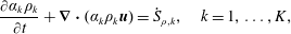
 $E=\unicode[STIX]{x1D70C}e+(1/2)\unicode[STIX]{x1D70C}\boldsymbol{u}^{2}$
and
$E=\unicode[STIX]{x1D70C}e+(1/2)\unicode[STIX]{x1D70C}\boldsymbol{u}^{2}$
and
 $e$
are the density, velocity, pressure, unit tensor, total energy and internal specific energy of the mixture, respectively. Three components are included, indicated by the subscripts
$e$
are the density, velocity, pressure, unit tensor, total energy and internal specific energy of the mixture, respectively. Three components are included, indicated by the subscripts
 $k$
can be 1, 2 or 3, which represent the vapour, liquid and air, respectively. The saturation constraint of the volume of fraction yields:
$k$
can be 1, 2 or 3, which represent the vapour, liquid and air, respectively. The saturation constraint of the volume of fraction yields:  $$\begin{eqnarray}\unicode[STIX]{x1D6FC}_{K}=1-\mathop{\sum }_{k=1}^{K-1}\unicode[STIX]{x1D6FC}_{k}.\end{eqnarray}$$
 ${\dot{S}}_{\unicode[STIX]{x1D70C},k}$
and
${\dot{S}}_{\unicode[STIX]{x1D70C},k}$
and
 ${\dot{S}}_{\unicode[STIX]{x1D6FC},k}$
are the source terms for the volume mass and volume fraction related to the phase transition, which can be respectively expressed as:
${\dot{S}}_{\unicode[STIX]{x1D6FC},k}$
are the source terms for the volume mass and volume fraction related to the phase transition, which can be respectively expressed as:
 $$\begin{eqnarray}{\dot{S}}_{\unicode[STIX]{x1D70C},1}={\dot{m}}=\unicode[STIX]{x1D708}(g_{2}-\unicode[STIX]{x1D707}_{1}),\quad {\dot{S}}_{\unicode[STIX]{x1D70C},2}=-{\dot{m}}=\unicode[STIX]{x1D708}(\unicode[STIX]{x1D707}_{1}-g_{2}),\quad {\dot{S}}_{\unicode[STIX]{x1D70C},3}=0,\end{eqnarray}$$
 $$\begin{eqnarray}{\dot{S}}_{\unicode[STIX]{x1D6FC},k}=\frac{{\dot{m}}}{\unicode[STIX]{x1D71A}_{k}}=\frac{\unicode[STIX]{x1D708}}{\unicode[STIX]{x1D71A}_{k}}(g_{2}-\unicode[STIX]{x1D707}_{1}),\quad k=1,2,\end{eqnarray}$$
where
 $\unicode[STIX]{x1D708}\,({\geqslant}0)$
is the relaxation parameter for the chemical potential,
$\unicode[STIX]{x1D708}\,({\geqslant}0)$
is the relaxation parameter for the chemical potential,
 $g_{2}$
is the Gibbs free energy of the liquid phase and
$g_{2}$
is the Gibbs free energy of the liquid phase and
 $\unicode[STIX]{x1D707}_{1}$
is the chemical potential of the vapour phase, respectively. In the present study, the parameter
$\unicode[STIX]{x1D707}_{1}$
is the chemical potential of the vapour phase, respectively. In the present study, the parameter
 $\unicode[STIX]{x1D708}$
is taken as infinite if the phase-transition condition is satisfied, otherwise it is zero. Therefore, the model is free of parameters. Formulas for the parameters
$\unicode[STIX]{x1D708}$
is taken as infinite if the phase-transition condition is satisfied, otherwise it is zero. Therefore, the model is free of parameters. Formulas for the parameters
 $\unicode[STIX]{x1D71A}_{k}$
can be found in Zein et al. (Reference Zein, Hantke and Warnecke2010, Reference Zein, Hantke and Warnecke2013). For details, please refer to the book of Müller & Müller (Reference Müller and Müller2009).
$\unicode[STIX]{x1D71A}_{k}$
can be found in Zein et al. (Reference Zein, Hantke and Warnecke2010, Reference Zein, Hantke and Warnecke2013). For details, please refer to the book of Müller & Müller (Reference Müller and Müller2009).
The thermodynamic state of the fluid is described by the stiffened gas equation of state (SG-EOS) (Saurel et al. Reference Saurel, Petitpas and Abgrall2008):
 $$\begin{eqnarray}\displaystyle & \displaystyle e_{k}(p,\unicode[STIX]{x1D70C}_{k})=\frac{p+\unicode[STIX]{x1D6FE}_{k}p_{\infty ,k}}{\unicode[STIX]{x1D70C}_{k}(\unicode[STIX]{x1D6FE}_{k}-1)}+q_{k}, & \displaystyle\end{eqnarray}$$
 $$\begin{eqnarray}\displaystyle & \displaystyle \unicode[STIX]{x1D70C}_{k}(p,T)=\frac{p+p_{\infty ,k}}{C_{v,k}T(\unicode[STIX]{x1D6FE}_{k}-1)}, & \displaystyle\end{eqnarray}$$
 $$\begin{eqnarray}\displaystyle & \displaystyle h_{k}(T)=\unicode[STIX]{x1D6FE}_{k}C_{v,k}T+q_{k}, & \displaystyle\end{eqnarray}$$
 $$\begin{eqnarray}\displaystyle & \displaystyle g_{k}(p,T)=(C_{v,k}\unicode[STIX]{x1D6FE}_{k}-q_{k}^{\prime })T-C_{v,k}T\log \frac{T^{\unicode[STIX]{x1D6FE}_{k}}}{(p+p_{\infty ,k})^{\unicode[STIX]{x1D6FE}_{k}-1}}+q_{k}, & \displaystyle\end{eqnarray}$$
 $$\begin{eqnarray}\displaystyle & \displaystyle \unicode[STIX]{x1D707}_{1}(T,g_{1},\unicode[STIX]{x1D6FC}_{1},\unicode[STIX]{x1D6FC}_{2})=g_{1}+(\unicode[STIX]{x1D6FE}_{1}-1)C_{v,1}T\log \frac{\unicode[STIX]{x1D6FC}_{1}}{1-\unicode[STIX]{x1D6FC}_{2}}, & \displaystyle\end{eqnarray}$$
where,
 $e_{k}$
,
$e_{k}$
,
 $h_{k}$
,
$h_{k}$
,
 $g_{k}$
and
$g_{k}$
and
 $\unicode[STIX]{x1D707}_{k}$
are respectively internal energy, enthalpy, Gibbs free energy and chemical potential of the considered component;
$\unicode[STIX]{x1D707}_{k}$
are respectively internal energy, enthalpy, Gibbs free energy and chemical potential of the considered component;
 $\unicode[STIX]{x1D6FE}_{k}$
,
$\unicode[STIX]{x1D6FE}_{k}$
,
 $p_{\infty ,k}$
,
$p_{\infty ,k}$
,
 $C_{v,k}$
,
$C_{v,k}$
,
 $q_{k}$
and
$q_{k}$
and
 $q_{k}^{\prime }$
are the specific heat ratio, material reference parameter with the dimension of pressure, specific heat capacity at constant volume, heat of formation and entropy constant. The corresponding values of these parameters are listed in table 1. The associated sound speed in each component fluid is given by
$q_{k}^{\prime }$
are the specific heat ratio, material reference parameter with the dimension of pressure, specific heat capacity at constant volume, heat of formation and entropy constant. The corresponding values of these parameters are listed in table 1. The associated sound speed in each component fluid is given by
 $c_{k}=\sqrt{(p_{k}+p_{\infty ,k})\unicode[STIX]{x1D6FE}_{k}/\unicode[STIX]{x1D70C}_{k}}$
.
$c_{k}=\sqrt{(p_{k}+p_{\infty ,k})\unicode[STIX]{x1D6FE}_{k}/\unicode[STIX]{x1D70C}_{k}}$
.
Table 1. The parameters involved in the SG-EOS (Han et al. Reference Han, Hantke and Müller2017).

The interface spreads over a few cells due to numerical diffusion in the interface capturing scheme. In this diffuse region, the mixture fluid variables are given as follows (Petitpas et al. Reference Petitpas, Franquet, Saurel and Le Metayer2007; Saurel et al. Reference Saurel, Petitpas and Abgrall2008; Zein et al. Reference Zein, Hantke and Warnecke2010):
 $$\begin{eqnarray}\displaystyle & \displaystyle \unicode[STIX]{x1D70C}=\mathop{\sum }_{k=1}^{K}\unicode[STIX]{x1D6FC}_{k}\unicode[STIX]{x1D70C}_{k}, & \displaystyle\end{eqnarray}$$
 $$\begin{eqnarray}\displaystyle & \displaystyle \unicode[STIX]{x1D70C}e=\mathop{\sum }_{k=1}^{K}\unicode[STIX]{x1D6FC}_{k}\unicode[STIX]{x1D70C}_{k}e_{k}, & \displaystyle\end{eqnarray}$$
 $$\begin{eqnarray}\displaystyle & \displaystyle p=\frac{\unicode[STIX]{x1D70C}e-\displaystyle \mathop{\sum }_{k=1}^{K}\unicode[STIX]{x1D6FC}_{k}\unicode[STIX]{x1D70C}_{k}q_{k}-\displaystyle \mathop{\sum }_{k=1}^{K}{\displaystyle \frac{\unicode[STIX]{x1D6FC}_{k}\unicode[STIX]{x1D6FE}_{k}p_{\infty ,k}}{\unicode[STIX]{x1D6FE}_{k}-1}}}{\displaystyle \mathop{\sum }_{k=1}^{K}{\displaystyle \frac{\unicode[STIX]{x1D6FC}_{k}}{\unicode[STIX]{x1D6FE}_{k}-1}}}, & \displaystyle\end{eqnarray}$$
 $$\begin{eqnarray}\displaystyle & \displaystyle c=\sqrt{\mathop{\sum }_{k=1}^{K}\frac{\unicode[STIX]{x1D6FC}_{k}\unicode[STIX]{x1D70C}_{k}}{\unicode[STIX]{x1D70C}}c_{k}^{2}}. & \displaystyle\end{eqnarray}$$
2.3 Numerical method
The finite volume method is used to discretize the governing equations, equation (2.4). A hybrid scheme (Titarev & Toro Reference Titarev and Toro2004), which combines the component-wise fifth-order weighted essentially non-oscillatory (WENO) scheme and a second-order monotone upstream centred scheme for conservation laws (MUSCL) scheme, is applied for the spatial reconstructions to the primitive variables. A Godunov-type Harten–Lax–van Leer contact (HLLC) approximate Riemann solver (Toro Reference Toro2013) is employed to solve the numerical flux at the edges of the cells. In order to adopt the HLLC Riemann solver, referring to the work of Johnsen & Colonius (Reference Johnsen and Colonius2006), the advection equation (2.4d ) is rewritten in a mathematically equivalent form with the chain rule. A third-order total variation diminishing (TVD) Runge–Kutta scheme (Gottlieb & Shu Reference Gottlieb and Shu1998) is utilized for time marching. The source terms, related to the phase transition, are decoupled from the hyperbolic operator, which will be explained in detail in the following section.
2.3.1 Numerical treatment for phase-transition source terms
For the present compressible two-phase problem, two different phase-transition patterns are involved, the vapour phase transforming into its liquid phase, and the liquid phase transforming into its vapour phase. The physical conditions that trigger the two different phase-transition patterns are introduced separately in this section.
For the vapour phase transforming into its liquid phase, the condition that triggers the phase transition is determined by
 $p>p_{sat}(T)$
, where
$p>p_{sat}(T)$
, where
 $p_{sat}(T)$
is the saturated pressure at temperature
$p_{sat}(T)$
is the saturated pressure at temperature
 $T$
. The equivalent condition is that the chemical potential
$T$
. The equivalent condition is that the chemical potential
 $\unicode[STIX]{x1D707}_{v}$
of the vapour phase is larger than the Gibbs free energy
$\unicode[STIX]{x1D707}_{v}$
of the vapour phase is larger than the Gibbs free energy
 $g_{l}$
of the liquid phase (Han et al.
Reference Han, Hantke and Müller2017). This is useful for the numerical treatment of the phase-transition source terms. For the liquid phase transforming into its vapour phase, a threshold pressure,
$g_{l}$
of the liquid phase (Han et al.
Reference Han, Hantke and Müller2017). This is useful for the numerical treatment of the phase-transition source terms. For the liquid phase transforming into its vapour phase, a threshold pressure,
 $p_{threshold}$
, is used to determine when the phase-transition process is triggered. In the present numerical study, with the assumption of pure water, only the homogeneous cavitation process is considered. The value of
$p_{threshold}$
, is used to determine when the phase-transition process is triggered. In the present numerical study, with the assumption of pure water, only the homogeneous cavitation process is considered. The value of
 $p_{threshold}$
is obtained by a linear approximation of the curve of the cavitation pressure of water over the temperature, as per Caupin & Herbert (Reference Caupin and Herbert2006). The mathematical expression is described as follows:
$p_{threshold}$
is obtained by a linear approximation of the curve of the cavitation pressure of water over the temperature, as per Caupin & Herbert (Reference Caupin and Herbert2006). The mathematical expression is described as follows:
 $$\begin{eqnarray}p_{threshold}=p_{ref,1}+(p_{ref,0}-p_{ref,1})\frac{(T-T_{ref,1})}{(T_{ref,0}-T_{ref,1})},\end{eqnarray}$$
where,
 $T$
is the fluid temperature (K),
$T$
is the fluid temperature (K),
 $T_{ref,0}$
and
$T_{ref,0}$
and
 $T_{ref,1}$
are the reference temperatures, taken as 273.15 K and 288.15 K, respectively, and
$T_{ref,1}$
are the reference temperatures, taken as 273.15 K and 288.15 K, respectively, and
 $p_{ref,0}$
and
$p_{ref,0}$
and
 $p_{ref,1}$
are the reference pressures, taken as
$p_{ref,1}$
are the reference pressures, taken as
 $-115.0~\text{MPa}$
and
$-115.0~\text{MPa}$
and
 $-100.0~\text{MPa}$
, respectively (Caupin & Herbert Reference Caupin and Herbert2006). When the local pressure is lower than
$-100.0~\text{MPa}$
, respectively (Caupin & Herbert Reference Caupin and Herbert2006). When the local pressure is lower than
 $p_{threshold}$
, the phase transition process is triggered.
$p_{threshold}$
, the phase transition process is triggered.
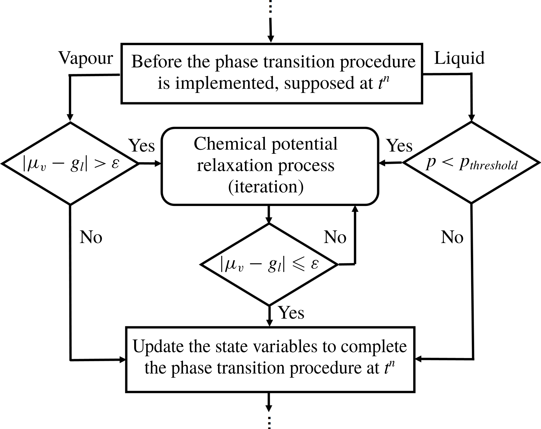
Figure 2. The treatment of the phase-transition procedure in the present numerical study.
Figure 2 shows the flow chart of the numerical treatment of the phase-transition source terms. When the phase-transition condition is satisfied, an instantaneous relaxation process is employed to find the variables in a thermodynamic equilibrium state. Referring to Han et al. (Reference Han, Hantke and Müller2017), relaxation based on the chemical potential is employed for the present numerical study, in which local thermodynamic equilibrium is achieved when
 $\unicode[STIX]{x1D707}_{v}=g_{l}$
. According to the conservation of total mass and total momentum, the Gibbs free energy of the liquid phase,
$\unicode[STIX]{x1D707}_{v}=g_{l}$
. According to the conservation of total mass and total momentum, the Gibbs free energy of the liquid phase,
 $g_{l}$
, and the chemical potential of the vapour phase,
$g_{l}$
, and the chemical potential of the vapour phase,
 $\unicode[STIX]{x1D707}_{v}$
, can both be expressed as a function of phasic density
$\unicode[STIX]{x1D707}_{v}$
, can both be expressed as a function of phasic density
 $\unicode[STIX]{x1D6FC}_{1}\unicode[STIX]{x1D70C}_{1}$
. The only unknown variable in the equation
$\unicode[STIX]{x1D6FC}_{1}\unicode[STIX]{x1D70C}_{1}$
. The only unknown variable in the equation
 $\unicode[STIX]{x1D707}_{v}(\unicode[STIX]{x1D6FC}_{1}\unicode[STIX]{x1D70C}_{1})=g_{l}(\unicode[STIX]{x1D6FC}_{1}\unicode[STIX]{x1D70C}_{1})$
is
$\unicode[STIX]{x1D707}_{v}(\unicode[STIX]{x1D6FC}_{1}\unicode[STIX]{x1D70C}_{1})=g_{l}(\unicode[STIX]{x1D6FC}_{1}\unicode[STIX]{x1D70C}_{1})$
is
 $\unicode[STIX]{x1D6FC}_{1}\unicode[STIX]{x1D70C}_{1}$
and an iteration procedure is applied to find its value. Then, the other variables can be obtained via their relationship with
$\unicode[STIX]{x1D6FC}_{1}\unicode[STIX]{x1D70C}_{1}$
and an iteration procedure is applied to find its value. Then, the other variables can be obtained via their relationship with
 $\unicode[STIX]{x1D6FC}_{1}\unicode[STIX]{x1D70C}_{1}$
. A small value
$\unicode[STIX]{x1D6FC}_{1}\unicode[STIX]{x1D70C}_{1}$
. A small value
 $\unicode[STIX]{x1D700}$
, chosen as
$\unicode[STIX]{x1D700}$
, chosen as
 $10^{-6}$
, is used to determine whether the iteration convergence is achieved, which is regarded as the thermodynamic equilibrium state from the numerical aspect. Consequently, the other variables at equilibrium state, including
$10^{-6}$
, is used to determine whether the iteration convergence is achieved, which is regarded as the thermodynamic equilibrium state from the numerical aspect. Consequently, the other variables at equilibrium state, including
 $p$
,
$p$
,
 $T$
and
$T$
and
 $\unicode[STIX]{x1D6FC}_{k}\unicode[STIX]{x1D70C}_{k}(k\neq 1)$
are obtained. For detailed derivations, readers can refer to Han et al. (Reference Han, Hantke and Müller2017).
$\unicode[STIX]{x1D6FC}_{k}\unicode[STIX]{x1D70C}_{k}(k\neq 1)$
are obtained. For detailed derivations, readers can refer to Han et al. (Reference Han, Hantke and Müller2017).
2.3.2 Boundary conditions and initialization
Figure 1 shows the configuration of the computational domain. The slip wall condition is employed for the bottom boundary of the computational domain, while the Thompson-type non-reflecting boundary condition (Thompson Reference Thompson1987) is employed for the remaining boundaries where only the outgoing waves are evaluated. The liquid and surrounding gas phase are initially in equilibrium with a temperature of 300 K (
 $T_{i}$
) and pressure of 1 atm (
$T_{i}$
) and pressure of 1 atm (
 $p_{i}$
). The initial velocity of the liquid column is changed for each case; however, the initial condition of the surrounding gas phase remains unchanged for all computation cases. Uniform grids are used for all computations, and the Courant–Friedrich–Lewis (CFL) number is taken as 0.4 for all cases.
$p_{i}$
). The initial velocity of the liquid column is changed for each case; however, the initial condition of the surrounding gas phase remains unchanged for all computation cases. Uniform grids are used for all computations, and the Courant–Friedrich–Lewis (CFL) number is taken as 0.4 for all cases.
3 Numerical verification
3.1 Grid sensitivity analysis
The grid sensitivity is analysed by choosing three different grid resolutions: 1.2 (grid-level I), 4.8 (grid-level II) and 10.8 million cells (grid-level III). The grid cells per column diameter correspond to 500, 1000 and 1500, respectively.
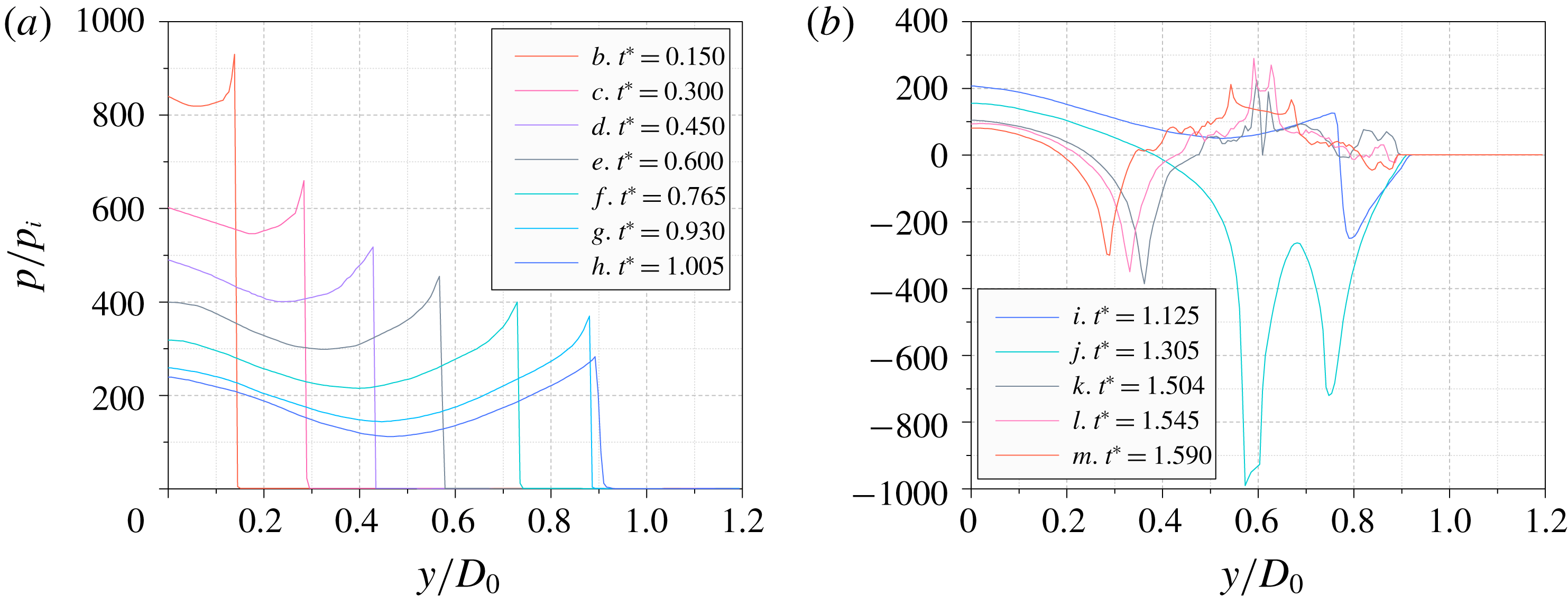
The pressure contours for the three different mesh levels at the same instant are shown in figure 3. The extracted pressure profiles along the vertical central axis (
 $y$
-axis) under three different grid resolutions are shown in figure 4, where pressure is normalized by the initial ambient pressure
$y$
-axis) under three different grid resolutions are shown in figure 4, where pressure is normalized by the initial ambient pressure
 $p_{i}$
, and the
$p_{i}$
, and the
 $y$
coordinate by the initial droplet diameter
$y$
coordinate by the initial droplet diameter
 $D_{0}$
.
$D_{0}$
.

Figure 3. Pressure contours under three different grid resolutions,
 $t=4.0~\unicode[STIX]{x03BC}\text{s}$
.
$t=4.0~\unicode[STIX]{x03BC}\text{s}$
.

Figure 4. Dimensionless pressure along the axial line under three grid resolutions,
 $t=4.0~\unicode[STIX]{x03BC}\text{s}$
.
$t=4.0~\unicode[STIX]{x03BC}\text{s}$
.
Similar distributions are noticed for the pressure contours of the three different mesh levels, figure 3. It can be found that an obvious pressure jump exists due to the confined shock wave (its generation mechanism will be discussed in the following section) for all three grid resolutions at the same position. Slight deviations from the pressure profile are observed behind the shock wave in grid-level I due to the low mesh resolution, while the pressure profiles overlap well for the other two higher grid resolutions. In order to balance the computational efficiency and mesh resolution, the grid level II is finally chosen in the present study.
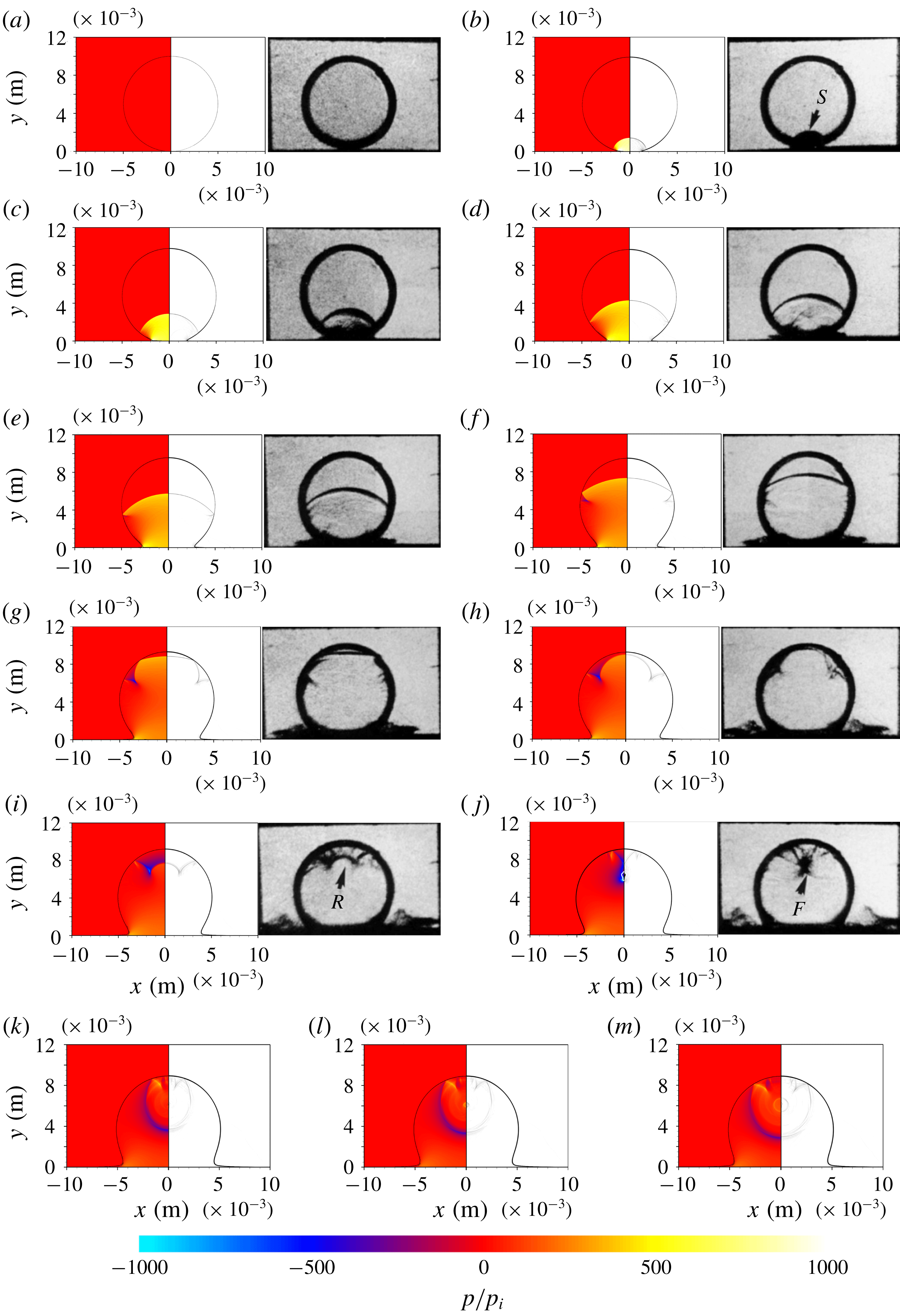
Figure 5. Numerical results of the pressure contours (left) and schlieren image (right) of a 10 mm water column impingement with initial speed of
 $110~\text{m}~\text{s}^{-1}$
at
$110~\text{m}~\text{s}^{-1}$
at
 $t=$
(a)
$t=$
(a)
 $0.0~\unicode[STIX]{x03BC}\text{s}$
, (b)
$0.0~\unicode[STIX]{x03BC}\text{s}$
, (b)
 $1.0~\unicode[STIX]{x03BC}\text{s}$
, (c)
$1.0~\unicode[STIX]{x03BC}\text{s}$
, (c)
 $2.0~\unicode[STIX]{x03BC}\text{s}$
, (d)
$2.0~\unicode[STIX]{x03BC}\text{s}$
, (d)
 $3.0~\unicode[STIX]{x03BC}\text{s}$
, (e)
$3.0~\unicode[STIX]{x03BC}\text{s}$
, (e)
 $4.0~\unicode[STIX]{x03BC}\text{s}$
, (f)
$4.0~\unicode[STIX]{x03BC}\text{s}$
, (f)
 $5.1~\unicode[STIX]{x03BC}\text{s}$
, (g)
$5.1~\unicode[STIX]{x03BC}\text{s}$
, (g)
 $6.2~\unicode[STIX]{x03BC}\text{s}$
, (h)
$6.2~\unicode[STIX]{x03BC}\text{s}$
, (h)
 $6.7~\unicode[STIX]{x03BC}\text{s}$
, (i)
$6.7~\unicode[STIX]{x03BC}\text{s}$
, (i)
 $7.5~\unicode[STIX]{x03BC}\text{s}$
, (j)
$7.5~\unicode[STIX]{x03BC}\text{s}$
, (j)
 $8.7~\unicode[STIX]{x03BC}\text{s}$
, (k)
$8.7~\unicode[STIX]{x03BC}\text{s}$
, (k)
 $10.0~\unicode[STIX]{x03BC}\text{s}$
, (l)
$10.0~\unicode[STIX]{x03BC}\text{s}$
, (l)
 $10.3~\unicode[STIX]{x03BC}\text{s}$
, (m)
$10.3~\unicode[STIX]{x03BC}\text{s}$
, (m)
 $10.6~\unicode[STIX]{x03BC}\text{s}$
(the cavitation zone extracted from the vapour volume fraction is marked with the solid line). Also shows the experimental schlieren images (a–j) with time interval of
$10.6~\unicode[STIX]{x03BC}\text{s}$
(the cavitation zone extracted from the vapour volume fraction is marked with the solid line). Also shows the experimental schlieren images (a–j) with time interval of
 $1~\unicode[STIX]{x03BC}\text{s}$
along the impact procedure of Field et al. (Reference Field, Dear and Ogren1989).
$1~\unicode[STIX]{x03BC}\text{s}$
along the impact procedure of Field et al. (Reference Field, Dear and Ogren1989).
3.2 Two-dimensional validation case
The two-dimensional cylindrical liquid column impaction is simulated. The parameters have the same values as in Field et al. (Reference Field, Dear and Ogren1989). The initial impinging velocity
 $V_{0}$
is
$V_{0}$
is
 $110~\text{m}~\text{s}^{-1}$
. Figure 5 shows the comparison between the present simulation results and the experimental results from Field et al. (Reference Field, Dear and Ogren1989). For the visualization of the numerical simulations, both the numerical schlieren and pressure contours are shown.
$110~\text{m}~\text{s}^{-1}$
. Figure 5 shows the comparison between the present simulation results and the experimental results from Field et al. (Reference Field, Dear and Ogren1989). For the visualization of the numerical simulations, both the numerical schlieren and pressure contours are shown.
The analysis begins when the column just impacts on the solid wall, figure 5(a). Subsequently, the confined shock wave (denoted by S in the experimental image) is generated due to the rapid pressure rising from the impaction region and it propagates downstream away from the initial bottom pole of the column, figure 5(b). From then on, the ending points of the confined shock wave propagate along the column surface and the shock wave passes through the water column. The confined shock wave finally touches the top pole of column (TP) until the time shown in figure 5(g). Meanwhile, the confined shock wave is reflected by the column surface as it propagates and a series of reflected rarefaction waves are generated. The rarefaction waves interact (denoted by R in the experimental image) and tend to be focused inside the water column due to the curved surface. As the rarefaction waves focus, the pressure of the local fluid becomes very low, figure 5(j). Once the local fluid pressure is lower than
 $p_{threshold}$
, a violent phase transition occurs. This phenomenon has been observed both in the experiments and simulations. The last figure obtained by the experiment, figure 5(j), shows that a cavitation zone is generated (denoted by the arrow F). For the numerical simulation results, a similar cavitation zone is recognized by the volume fraction of vapour, marked by the solid line shown on the left-hand side of figure 5(j). The detailed analysis of the convergence of the reflected rarefaction waves and the generation of cavitation will be presented in the next section.
$p_{threshold}$
, a violent phase transition occurs. This phenomenon has been observed both in the experiments and simulations. The last figure obtained by the experiment, figure 5(j), shows that a cavitation zone is generated (denoted by the arrow F). For the numerical simulation results, a similar cavitation zone is recognized by the volume fraction of vapour, marked by the solid line shown on the left-hand side of figure 5(j). The detailed analysis of the convergence of the reflected rarefaction waves and the generation of cavitation will be presented in the next section.
Furthermore, the simulation can predict the successive flow process after cavitation occurs. As the droplet continually moves towards the wall, the cavitation collapses as shown from figure 5(k) to figure 5(m). Figure 5(k) corresponds to the time when the cavitation zone has completely collapsed, while figure 5(l) and figure 5(m) show the induced circular shock wave due to the collapse of the cavity. Overall, the simulation results, demonstrating the droplet impinging process, show a good agreement with the experimental flow visualization. The dynamical process of the cavity collapse will be analysed in detail in the next section.
The above comparison shows that the present mathematical models and numerical procedures are able to solve the problem of a cylindrical droplet impinging upon a solid wall. Moreover, the cavitation inception and subsequent collapse that occurs in the impaction process can be well captured by current computation capabilities.
4 Analysis of high-speed impingement of a water column
In this section, a detailed analysis is performed for the water column impingement. The analysis is based on the simulated results obtained when the initial impaction velocity of the cylindrical droplet is
 $110~\text{m}~\text{s}^{-1}$
, see § 3.2. In order to understand the physical mechanisms of the flow phenomena, the whole impaction process is divided into two stages, mainly according to the flow characteristics. The propagation and status of the confined shock wave inside the droplet is the main reason for the division of the flow process. In the first stage, the confined shock wave is generated and propagates inside the column (figure 5
b–g). The first stage ends when the confined shock wave touches the top pole of the column. The second stage (figure 5
h–m) begins and the cavitation inception and collapsing process take place.
$110~\text{m}~\text{s}^{-1}$
, see § 3.2. In order to understand the physical mechanisms of the flow phenomena, the whole impaction process is divided into two stages, mainly according to the flow characteristics. The propagation and status of the confined shock wave inside the droplet is the main reason for the division of the flow process. In the first stage, the confined shock wave is generated and propagates inside the column (figure 5
b–g). The first stage ends when the confined shock wave touches the top pole of the column. The second stage (figure 5
h–m) begins and the cavitation inception and collapsing process take place.
The dimensionless time
 $t^{\ast }$
is used, which is the ratio of the physical time over the characteristic time
$t^{\ast }$
is used, which is the ratio of the physical time over the characteristic time
 $\unicode[STIX]{x1D70F}$
(
$\unicode[STIX]{x1D70F}$
(
 $\unicode[STIX]{x1D70F}=D_{0}/c_{0}$
,
$\unicode[STIX]{x1D70F}=D_{0}/c_{0}$
,
 $D_{0}$
is the initial droplet diameter and
$D_{0}$
is the initial droplet diameter and
 $c_{0}$
is the sound speed of the droplet liquid under the initial condition), namely,
$c_{0}$
is the sound speed of the droplet liquid under the initial condition), namely,
 $t^{\ast }=t/\unicode[STIX]{x1D70F}$
. The pressure is non-dimensionalized by the initial ambient pressure
$t^{\ast }=t/\unicode[STIX]{x1D70F}$
. The pressure is non-dimensionalized by the initial ambient pressure
 $p_{i}$
. Figure 6 shows the pressure distributions along the vertical central axis inside the water column for the different stages respectively. Figure 6(a) corresponds to the time instants of figure 5(b–h) in the first stage. Figure 6(b) corresponds to the following series in the second stage.
$p_{i}$
. Figure 6 shows the pressure distributions along the vertical central axis inside the water column for the different stages respectively. Figure 6(a) corresponds to the time instants of figure 5(b–h) in the first stage. Figure 6(b) corresponds to the following series in the second stage.


4.1 The first stage
The first stage begins at
 $t_{0}$
when the water column just impacts the solid wall. There is a contact line segment
$t_{0}$
when the water column just impacts the solid wall. There is a contact line segment
 $\overline{AA^{\prime }}$
between the water column and the solid wall and
$\overline{AA^{\prime }}$
between the water column and the solid wall and
 $A$
coincides with
$A$
coincides with
 $A^{\prime }$
at
$A^{\prime }$
at
 $t_{0}$
. Furthermore, we only considered the left contact point
$t_{0}$
. Furthermore, we only considered the left contact point
 $A$
for the following analysis because flow is symmetric. It is obvious that
$A$
for the following analysis because flow is symmetric. It is obvious that
 $A$
is moving with velocity
$A$
is moving with velocity
 $V_{A}$
along the
$V_{A}$
along the
 $x$
-axis during the impaction of the column. The contact angle
$x$
-axis during the impaction of the column. The contact angle
 $\unicode[STIX]{x1D703}$
is defined as the angle between the solid wall and the tangent line of the liquid column at
$\unicode[STIX]{x1D703}$
is defined as the angle between the solid wall and the tangent line of the liquid column at
 $A$
. The value of
$A$
. The value of
 $\unicode[STIX]{x1D703}$
is zero when the water column just impacts the solid wall, and
$\unicode[STIX]{x1D703}$
is zero when the water column just impacts the solid wall, and
 $V_{A}$
is much higher than the local liquid sound speed at this time. By the Huygens principle (Haller et al.
Reference Haller, Poulikakos, Ventikos and Monkewitz2003), at each time instant, an individual compression wavelet will be emitted at
$V_{A}$
is much higher than the local liquid sound speed at this time. By the Huygens principle (Haller et al.
Reference Haller, Poulikakos, Ventikos and Monkewitz2003), at each time instant, an individual compression wavelet will be emitted at
 $A$
that will propagate with the local sound speed. Accounting for the acoustic limit (Lesser Reference Lesser1981) of the compression wavelet,
$A$
that will propagate with the local sound speed. Accounting for the acoustic limit (Lesser Reference Lesser1981) of the compression wavelet,
 $V_{A}$
is higher than the propagation speed of the wavelet at the early stage of the impaction, which means that the emitted compression wavelets cannot exceed the contact point
$V_{A}$
is higher than the propagation speed of the wavelet at the early stage of the impaction, which means that the emitted compression wavelets cannot exceed the contact point
 $A$
.
$A$
.
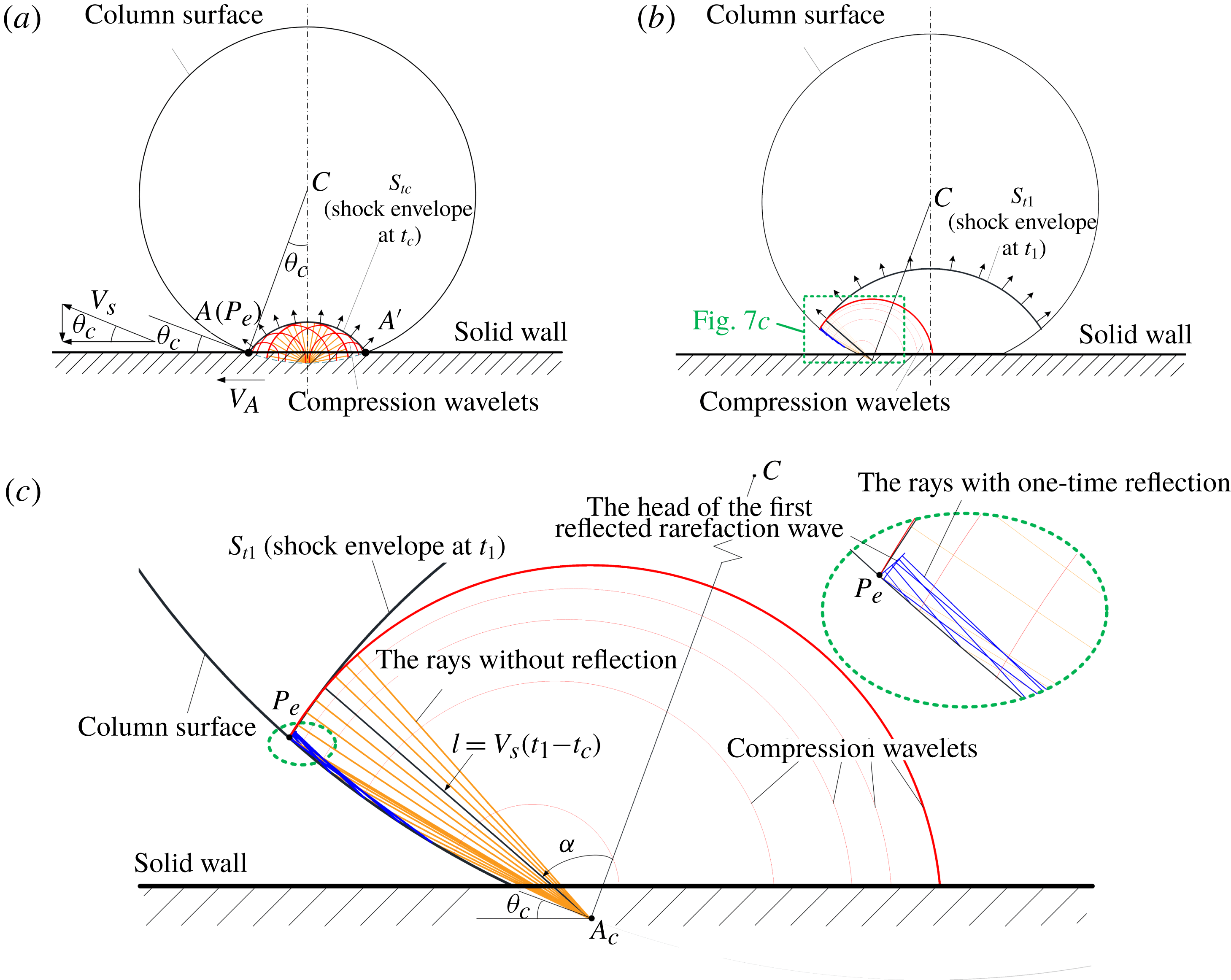
Figure 7. Schematic diagram of the generation of confined shock and the ray analysis: (a) the schematic diagram at critical time
 $t_{c}$
; (b) the schematic diagram at the time instant,
$t_{c}$
; (b) the schematic diagram at the time instant,
 $t_{1}$
, which is selected at the instant after the critical time; (c) the enlarged view of the schematic diagram at
$t_{1}$
, which is selected at the instant after the critical time; (c) the enlarged view of the schematic diagram at
 $t_{1}$
(
$t_{1}$
(
 $\overline{CA_{c}}$
is the line between the critical contact point
$\overline{CA_{c}}$
is the line between the critical contact point
 $A_{c}$
and the water column centre
$A_{c}$
and the water column centre
 $C$
).
$C$
).
These compression wavelets form a shock envelope, denoted as
 $S_{t}$
, figure 7(a). As the shock wave is constrained inside the column, this shock envelope
$S_{t}$
, figure 7(a). As the shock wave is constrained inside the column, this shock envelope
 $S_{t}$
is also called a confined shock (Obreschkow et al.
Reference Obreschkow, Dorsaz, Kobel, de Bosset, Tinguely, Field and Farhat2011). Initially, the ending point of the confined shock (denoted as
$S_{t}$
is also called a confined shock (Obreschkow et al.
Reference Obreschkow, Dorsaz, Kobel, de Bosset, Tinguely, Field and Farhat2011). Initially, the ending point of the confined shock (denoted as
 $P_{e}$
) remains attached to the solid wall and overlaps with
$P_{e}$
) remains attached to the solid wall and overlaps with
 $A$
. Since
$A$
. Since
 $V_{A}$
decreases gradually, the
$V_{A}$
decreases gradually, the
 $x$
-component velocity of
$x$
-component velocity of
 $P_{e}$
will catch up with
$P_{e}$
will catch up with
 $V_{A}$
and the confined shock will detach itself from the solid wall. We define the time when the confined shock just detaches itself from the solid wall as the critical time
$V_{A}$
and the confined shock will detach itself from the solid wall. We define the time when the confined shock just detaches itself from the solid wall as the critical time
 $t_{c}$
. If
$t_{c}$
. If
 $t<t_{c}$
, the end points of the shock envelope are attached to the solid wall and
$t<t_{c}$
, the end points of the shock envelope are attached to the solid wall and
 $P_{e}$
overlaps with
$P_{e}$
overlaps with
 $A$
. If
$A$
. If
 $t>t_{c}$
, the shock envelope will detach itself from the solid wall and
$t>t_{c}$
, the shock envelope will detach itself from the solid wall and
 $P_{e}$
will propagate along the column surface above the solid wall. At the critical time
$P_{e}$
will propagate along the column surface above the solid wall. At the critical time
 $t_{c}$
, the critical contact angle
$t_{c}$
, the critical contact angle
 $\unicode[STIX]{x1D703}_{c}$
at the critical contact point
$\unicode[STIX]{x1D703}_{c}$
at the critical contact point
 $A_{c}$
is derived from the following expression (Rein Reference Rein1993):
$A_{c}$
is derived from the following expression (Rein Reference Rein1993):
 $$\begin{eqnarray}\tan \unicode[STIX]{x1D703}_{c}=\frac{V_{0}}{V_{A,c}}=\frac{V_{0}}{\sqrt{{V_{s}}^{2}-V_{0}^{2}}},\end{eqnarray}$$
where
 $V_{A,c}$
is the velocity of
$V_{A,c}$
is the velocity of
 $A_{c}$
and
$A_{c}$
and
 $V_{s}$
is the velocity of
$V_{s}$
is the velocity of
 $P_{e}$
, obtained from Heymann (Reference Heymann1969), which yields:
$P_{e}$
, obtained from Heymann (Reference Heymann1969), which yields:
 $$\begin{eqnarray}V_{s}=c_{0}+\unicode[STIX]{x1D712}V_{0},\end{eqnarray}$$
where
 $c_{0}$
is the sound speed of the liquid in the unshocked region and
$c_{0}$
is the sound speed of the liquid in the unshocked region and
 $\unicode[STIX]{x1D712}$
is a constant that depends on the liquid property. For water,
$\unicode[STIX]{x1D712}$
is a constant that depends on the liquid property. For water,
 $\unicode[STIX]{x1D712}$
is taken as 2.0 according to Heymann (Reference Heymann1969) and 1.921 according to Haller et al. (Reference Haller, Ventikos, Poulikakos and Monkewitz2002). Both values of
$\unicode[STIX]{x1D712}$
is taken as 2.0 according to Heymann (Reference Heymann1969) and 1.921 according to Haller et al. (Reference Haller, Ventikos, Poulikakos and Monkewitz2002). Both values of
 $\unicode[STIX]{x1D712}$
are very close to each other in these two references, however, in this study we assume the value suggested by Heymann (Reference Heymann1969). Subsequently, the critical angle
$\unicode[STIX]{x1D712}$
are very close to each other in these two references, however, in this study we assume the value suggested by Heymann (Reference Heymann1969). Subsequently, the critical angle
 $\unicode[STIX]{x1D703}_{c}$
calculated from (4.1) is
$\unicode[STIX]{x1D703}_{c}$
calculated from (4.1) is
 $3.6^{\circ }$
(
$3.6^{\circ }$
(
 $V_{0}=110~\text{m}~\text{s}^{-1}$
). Referring to Heymann (Reference Heymann1969), the water hammer pressure, the maximum pressure at the initial impact point
$V_{0}=110~\text{m}~\text{s}^{-1}$
). Referring to Heymann (Reference Heymann1969), the water hammer pressure, the maximum pressure at the initial impact point
 $(O)$
, is defined as:
$(O)$
, is defined as:
 $$\begin{eqnarray}p_{h}=\unicode[STIX]{x1D70C}_{0}V_{0}V_{s},\end{eqnarray}$$
where
 $V_{s}$
is the velocity of the initial confined shock wave, calculated by (4.2).
$V_{s}$
is the velocity of the initial confined shock wave, calculated by (4.2).
It is inferred from figure 6(a) that the confined shock propagates upward, and its strength gradually decreases as it detaches from the solid wall. The confined shock can be equivalent to an explosion wave with a certain arc length whose strength gradually decreases as it propagates outwards.
As the ending points of the confined shock wave detach from the solid wall, the shock wave propagates inside the water column and moves towards the top pole, as shown in figure 7(b). The reflected and transmitted waves are generated on the curved column surface. Since the acoustic impedance
 $\unicode[STIX]{x1D70C}_{l}c_{l}$
in water is much larger than that in air, the reflected waves should be rarefaction waves and the transmitted waves should be shock waves. The transmitted shock wave is so weak that it is almost invisible in the numerical schlieren images.
$\unicode[STIX]{x1D70C}_{l}c_{l}$
in water is much larger than that in air, the reflected waves should be rarefaction waves and the transmitted waves should be shock waves. The transmitted shock wave is so weak that it is almost invisible in the numerical schlieren images.
The path of the rays tracing the compression wavelets is demonstrated to understand the evolution of different types of waves. In figure 7(a), a series of rays pointed in different specified directions is used to demonstrate the evolution of each compression wavelet emitted from the contact point. From one contact point, the rays represent the paths of the compression wavelet and the length of the rays is equal to the propagation distance of the compression wavelet. Meanwhile, the rays will be reflected symmetrically on the curved column surface. In this stage, the situation at the critical time
 $t_{c}$
is chosen to analyse the rays emitted from the contact point
$t_{c}$
is chosen to analyse the rays emitted from the contact point
 $A_{c}$
, figure 7(a), which emits the last compression wavelet that can catch up with the confined shock. This wavelet propagates upwards for a certain time, for example at time instant
$A_{c}$
, figure 7(a), which emits the last compression wavelet that can catch up with the confined shock. This wavelet propagates upwards for a certain time, for example at time instant
 $t_{1}$
, and the wave structures and the emitted rays are shown in figure 7(b).
$t_{1}$
, and the wave structures and the emitted rays are shown in figure 7(b).
In figure 7(c), which is the intersection angle, the emitting angle of each ray is the angle between any arbitrarily chosen ray and the line segment
 $\overline{CA_{c}}$
. We can use the dimension of such an angle to analyse the reflection behaviour of the traced wavelet. The emitting angle
$\overline{CA_{c}}$
. We can use the dimension of such an angle to analyse the reflection behaviour of the traced wavelet. The emitting angle
 $\unicode[STIX]{x1D6FC}$
lies in
$\unicode[STIX]{x1D6FC}$
lies in
 $[0,\unicode[STIX]{x03C0}/2]$
. At a specific instant,
$[0,\unicode[STIX]{x03C0}/2]$
. At a specific instant,
 $t_{1}$
, the range of the ray
$t_{1}$
, the range of the ray
 $l$
is computed by
$l$
is computed by
 $l=c(t_{1}-t_{c})$
, where
$l=c(t_{1}-t_{c})$
, where
 $c$
is the local sound speed. If the compression wavelet is reflected from the column surface,
$c$
is the local sound speed. If the compression wavelet is reflected from the column surface,
 $l$
will represent the total range of the ray before and after reflection. The compression wavelet will be reflected more than once from the column surface. The reflection times are related to the angular dimension of
$l$
will represent the total range of the ray before and after reflection. The compression wavelet will be reflected more than once from the column surface. The reflection times are related to the angular dimension of
 $\unicode[STIX]{x1D6FC}$
and the present time, which are elaborated as follows:
$\unicode[STIX]{x1D6FC}$
and the present time, which are elaborated as follows:
If the emitted rays are not reflected at an instant
 $t$
, the emitting angle
$t$
, the emitting angle
 $\unicode[STIX]{x1D6FC}$
will satisfy:
$\unicode[STIX]{x1D6FC}$
will satisfy:
 $$\begin{eqnarray}\unicode[STIX]{x1D6FC}\leqslant \arccos \frac{l}{2R}=\arccos \frac{c(t-t_{\text{c}})}{2R}.\end{eqnarray}$$
If the rays are reflected
 $N$
times (
$N$
times (
 $N=1,2,3,\ldots$
), angle
$N=1,2,3,\ldots$
), angle
 $\unicode[STIX]{x1D6FC}$
will satisfy:
$\unicode[STIX]{x1D6FC}$
will satisfy:
 $$\begin{eqnarray}\arccos \frac{c(t-t_{\text{c}})}{2RN}=\arccos \frac{l/N}{2R}<\unicode[STIX]{x1D6FC}\leqslant \arccos \frac{l/(N+1)}{2R}=\arccos \frac{c(t-t_{\text{c}})}{2R(N+1)}.\end{eqnarray}$$
Thus, different intervals of the angle
 $\unicode[STIX]{x1D6FC}$
, according to the reflection times of a ray, exist.
$\unicode[STIX]{x1D6FC}$
, according to the reflection times of a ray, exist.

Figure 8. Computational results and the schematic diagram of ray analysis in the first stage at the time instant,
 $t^{\ast }=0.81(t_{2})$
: (a) the numerical schlieren contour; (b) the schematic diagram of ray analysis; (c) the partial enlarged view of the area of the dashed rectangle in figure 8(a,b). The left side presents the comparison between schematic diagram and numerical schlieren contour, while the right side presents the corresponding numerical result of pressure isolines.
$t^{\ast }=0.81(t_{2})$
: (a) the numerical schlieren contour; (b) the schematic diagram of ray analysis; (c) the partial enlarged view of the area of the dashed rectangle in figure 8(a,b). The left side presents the comparison between schematic diagram and numerical schlieren contour, while the right side presents the corresponding numerical result of pressure isolines.
The shock envelope is formed by the infinite emitted compression wavelets before the critical time
 $t_{c}$
. The compression wavelet emitted from the critical contact point
$t_{c}$
. The compression wavelet emitted from the critical contact point
 $A_{c}$
is part of the confined shock envelope and it is the nearest wavelet to the column surface. The reflection of this compression wavelet also represents the reflection of the confined shock on the column surface. The discussion about the evolution of this compression wavelet is helpful to understand the character of the confined shock wave close to the column surface. The rays that belong to this compression wavelet start to be reflected on the column surface once they are emitted from the critical contact point
$A_{c}$
is part of the confined shock envelope and it is the nearest wavelet to the column surface. The reflection of this compression wavelet also represents the reflection of the confined shock on the column surface. The discussion about the evolution of this compression wavelet is helpful to understand the character of the confined shock wave close to the column surface. The rays that belong to this compression wavelet start to be reflected on the column surface once they are emitted from the critical contact point
 $A_{c}$
. For
$A_{c}$
. For
 $\unicode[STIX]{x1D6FC}\in (\arccos (c(t_{1}-t_{c})/2R),\arccos (c(t_{1}-t_{c})/4R)]$
, the rays will be reflected once, and their ending points represent the head of the first reflection waves (the rarefaction waves), figure 7(c). Similarly, for
$\unicode[STIX]{x1D6FC}\in (\arccos (c(t_{1}-t_{c})/2R),\arccos (c(t_{1}-t_{c})/4R)]$
, the rays will be reflected once, and their ending points represent the head of the first reflection waves (the rarefaction waves), figure 7(c). Similarly, for
 $\unicode[STIX]{x1D6FC}\in (\arccos (c(t_{1}-t_{c})/4R),\arccos (c(t_{1}-t_{c})/6R)]$
, the rays will be reflected twice, and their ending points represent the head of the second reflection waves (the compression waves). Thus, the position of the head of the
$\unicode[STIX]{x1D6FC}\in (\arccos (c(t_{1}-t_{c})/4R),\arccos (c(t_{1}-t_{c})/6R)]$
, the rays will be reflected twice, and their ending points represent the head of the second reflection waves (the compression waves). Thus, the position of the head of the
 $N$
th reflection waves are known.
$N$
th reflection waves are known.
Meanwhile, as the water column continues to impact on the solid wall later than the critical time
 $t_{c}$
, compression wavelets are continuously generated, however, they never catch up with the confined shock envelope, figure 7(c). The behaviour of these compression wavelets is similar and their strength becomes very weak. Nonetheless, we will not elaborate further on this in the present study.
$t_{c}$
, compression wavelets are continuously generated, however, they never catch up with the confined shock envelope, figure 7(c). The behaviour of these compression wavelets is similar and their strength becomes very weak. Nonetheless, we will not elaborate further on this in the present study.
As the confined shock wave propagates upwards, the reflected rarefaction waves are observed behind the confined shock and a certain time,
 $t^{\ast }=0.81(t_{2})$
, is chosen for the following analysis. The numerical schlieren, the pressure contour together with the schematic of the emitted rays belonging to the compression wavelet, are shown in figure 8. The position and shape of the reflected rarefaction waves are obtained from the analysis of the emitted rays.
$t^{\ast }=0.81(t_{2})$
, is chosen for the following analysis. The numerical schlieren, the pressure contour together with the schematic of the emitted rays belonging to the compression wavelet, are shown in figure 8. The position and shape of the reflected rarefaction waves are obtained from the analysis of the emitted rays.
Figure 8(b) shows the emitted rays that belong to the non-reflected confined shock, the first reflected rarefaction, and the second reflected compression wave. Five regimes of the emitted rays exist, figure 8(b), which are divided based on the value range of the emitting angle
 $\unicode[STIX]{x1D6FC}$
, including (I),
$\unicode[STIX]{x1D6FC}$
, including (I),
 $0<\unicode[STIX]{x1D6FC}\leqslant \unicode[STIX]{x1D6FC}_{0}$
; (II),
$0<\unicode[STIX]{x1D6FC}\leqslant \unicode[STIX]{x1D6FC}_{0}$
; (II),
 $\unicode[STIX]{x1D6FC}_{0}<\unicode[STIX]{x1D6FC}\leqslant \unicode[STIX]{x1D6FC}_{1}$
; (III),
$\unicode[STIX]{x1D6FC}_{0}<\unicode[STIX]{x1D6FC}\leqslant \unicode[STIX]{x1D6FC}_{1}$
; (III),
 $\unicode[STIX]{x1D6FC}_{1}<\unicode[STIX]{x1D6FC}\leqslant \unicode[STIX]{x1D6FC}_{2}$
; (IV),
$\unicode[STIX]{x1D6FC}_{1}<\unicode[STIX]{x1D6FC}\leqslant \unicode[STIX]{x1D6FC}_{2}$
; (IV),
 $\unicode[STIX]{x1D6FC}_{2}<\unicode[STIX]{x1D6FC}\leqslant \unicode[STIX]{x1D6FC}_{3}$
; and (V),
$\unicode[STIX]{x1D6FC}_{2}<\unicode[STIX]{x1D6FC}\leqslant \unicode[STIX]{x1D6FC}_{3}$
; and (V),
 $\unicode[STIX]{x1D6FC}_{3}<\unicode[STIX]{x1D6FC}\leqslant \unicode[STIX]{x1D6FC}_{4}$
. In regimes (II) and (III) the emitted rays are reflected once and in regimes (IV) and (V) the emitted rays are reflected twice. As shown in figure 8(c), in regime (I),
$\unicode[STIX]{x1D6FC}_{3}<\unicode[STIX]{x1D6FC}\leqslant \unicode[STIX]{x1D6FC}_{4}$
. In regimes (II) and (III) the emitted rays are reflected once and in regimes (IV) and (V) the emitted rays are reflected twice. As shown in figure 8(c), in regime (I),
 $\unicode[STIX]{x1D6FC}_{0}=\arccos (c(t_{2}-t_{c})/2R)$
according to (4.4), the propagating head of these continuously emitted rays forms the confined shock envelope (
$\unicode[STIX]{x1D6FC}_{0}=\arccos (c(t_{2}-t_{c})/2R)$
according to (4.4), the propagating head of these continuously emitted rays forms the confined shock envelope (
 $S_{t}$
). In regime (II), the value of
$S_{t}$
). In regime (II), the value of
 $\unicode[STIX]{x1D6FC}_{1}$
lies between
$\unicode[STIX]{x1D6FC}_{1}$
lies between
 $\unicode[STIX]{x1D6FC}_{0}$
and
$\unicode[STIX]{x1D6FC}_{0}$
and
 $\unicode[STIX]{x1D6FC}_{2}$
and the propagating head of the continuously emitted rays forms the upper branch of the head of the first reflected rarefaction waves (
$\unicode[STIX]{x1D6FC}_{2}$
and the propagating head of the continuously emitted rays forms the upper branch of the head of the first reflected rarefaction waves (
 $\text{RRW}_{ub1}$
). In regime (III),
$\text{RRW}_{ub1}$
). In regime (III),
 $\unicode[STIX]{x1D6FC}_{2}=\arccos (c(t_{2}-t_{c})/4R)$
according to (4.5), the propagating head of the continuously emitted rays forms the lower branch of the head of the first reflected rarefaction waves (
$\unicode[STIX]{x1D6FC}_{2}=\arccos (c(t_{2}-t_{c})/4R)$
according to (4.5), the propagating head of the continuously emitted rays forms the lower branch of the head of the first reflected rarefaction waves (
 $\text{RRW}_{lb1}$
). In regime (IV), the value of
$\text{RRW}_{lb1}$
). In regime (IV), the value of
 $\unicode[STIX]{x1D6FC}_{3}$
lies between
$\unicode[STIX]{x1D6FC}_{3}$
lies between
 $\unicode[STIX]{x1D6FC}_{2}$
and
$\unicode[STIX]{x1D6FC}_{2}$
and
 $\unicode[STIX]{x1D6FC}_{4}$
and the propagating head of these continuous emitted rays forms the upper branch of the second reflected compression waves (
$\unicode[STIX]{x1D6FC}_{4}$
and the propagating head of these continuous emitted rays forms the upper branch of the second reflected compression waves (
 $\text{RCW}_{ub2}$
). In regime (V),
$\text{RCW}_{ub2}$
). In regime (V),
 $\unicode[STIX]{x1D6FC}_{4}=\arccos (c(t_{2}-t_{\text{c}})/6R)$
according to (4.5), the propagating head of the continuously emitted rays forms the lower branch of the second reflected compression waves (
$\unicode[STIX]{x1D6FC}_{4}=\arccos (c(t_{2}-t_{\text{c}})/6R)$
according to (4.5), the propagating head of the continuously emitted rays forms the lower branch of the second reflected compression waves (
 $\text{RCW}_{lb2}$
).
$\text{RCW}_{lb2}$
).
The analytical shape and position of the first reflected rarefaction waves (
 $\text{RRW}_{ub1}$
and
$\text{RRW}_{ub1}$
and
 $\text{RRW}_{lb1}$
) overlap well with those visualized by the numerical schlieren results, figure 8(c). The second reflected compression waves are too weak to be observed from the numerical schlieren results. From the pressure isolines, figure 8(c), the marked local maximum pressure region validates the second reflected compression waves and its location is also consistent with the analytical results. Ideally, the emitted rays can be reflected infinite number of times, while the other generated reflected waves are much weaker except for the first and second reflected waves. Therefore, they cannot be recognized in the numerical schlieren contour or in the pressure isolines.
$\text{RRW}_{lb1}$
) overlap well with those visualized by the numerical schlieren results, figure 8(c). The second reflected compression waves are too weak to be observed from the numerical schlieren results. From the pressure isolines, figure 8(c), the marked local maximum pressure region validates the second reflected compression waves and its location is also consistent with the analytical results. Ideally, the emitted rays can be reflected infinite number of times, while the other generated reflected waves are much weaker except for the first and second reflected waves. Therefore, they cannot be recognized in the numerical schlieren contour or in the pressure isolines.
In addition, due to the superposition of the first reflected rarefaction waves, and also indicated by the emitted rays, a local minimum-pressure region is observed, figure 8(c). Meanwhile, the pressure behind the lower branch of the first reflected rarefaction waves is recovered, because the subsequent emitting compression wavelets catch up with these rarefaction waves.
4.2 The second stage
The second stage begins when the confined shock
 $S_{t}$
reaches the TP of the water column at the time instant
$S_{t}$
reaches the TP of the water column at the time instant
 $t^{\ast }=0.975(t_{3})$
. The analytical schematic is presented in figure 9, which demonstrates the first reflected rarefaction wave evolution. The numerical schlieren contours at
$t^{\ast }=0.975(t_{3})$
. The analytical schematic is presented in figure 9, which demonstrates the first reflected rarefaction wave evolution. The numerical schlieren contours at
 $t^{\ast }=0.975(t_{3})$
and
$t^{\ast }=0.975(t_{3})$
and
 $t^{\ast }=1.305(t_{4})$
are shown in figures 9(b) and 9(d), respectively.
$t^{\ast }=1.305(t_{4})$
are shown in figures 9(b) and 9(d), respectively.
When all the rays initially emitted from BP are drawn, which are reflected once, the envelope of these first reflected rays is obtained, figure 9(a). The intersection points of
 $\text{RRW}_{ub1}$
and
$\text{RRW}_{ub1}$
and
 $\text{RRW}_{lb1}$
always lie on this envelope upon propagation of the reflected rarefaction wave. From the schematic of
$\text{RRW}_{lb1}$
always lie on this envelope upon propagation of the reflected rarefaction wave. From the schematic of
 $\text{RRW}_{ub1}$
and
$\text{RRW}_{ub1}$
and
 $\text{RRW}_{lb1}$
at four different time instants, which can be derived from similar analysis in § 4.1, it is observed that the intersection points of
$\text{RRW}_{lb1}$
at four different time instants, which can be derived from similar analysis in § 4.1, it is observed that the intersection points of
 $\text{RRW}_{ub1}$
and
$\text{RRW}_{ub1}$
and
 $\text{RRW}_{lb1}$
move along the envelope from time
$\text{RRW}_{lb1}$
move along the envelope from time
 $t_{2}$
to
$t_{2}$
to
 $t_{3}$
. When the uppermost point of the confined shock arrives at TP of the water column, the confined shock is totally reflected. The two branches of
$t_{3}$
. When the uppermost point of the confined shock arrives at TP of the water column, the confined shock is totally reflected. The two branches of
 $\text{RRW}_{ub1}$
, from the left and right sides, meet at the vertical central axis and an arched
$\text{RRW}_{ub1}$
, from the left and right sides, meet at the vertical central axis and an arched
 $\text{RRW}_{ub1}$
is formed with the two
$\text{RRW}_{ub1}$
is formed with the two
 $\text{RRW}_{lb1}$
following on the left and right sides. The propagating directions of the combined arched
$\text{RRW}_{lb1}$
following on the left and right sides. The propagating directions of the combined arched
 $\text{RRW}_{ub1}$
and the two separated
$\text{RRW}_{ub1}$
and the two separated
 $\text{RRW}_{lb1}$
from the left and right sides are shown in figure 9(b). This indicates that the combined arched
$\text{RRW}_{lb1}$
from the left and right sides are shown in figure 9(b). This indicates that the combined arched
 $\text{RRW}_{ub1}$
focuses inside the water column.
$\text{RRW}_{ub1}$
focuses inside the water column.
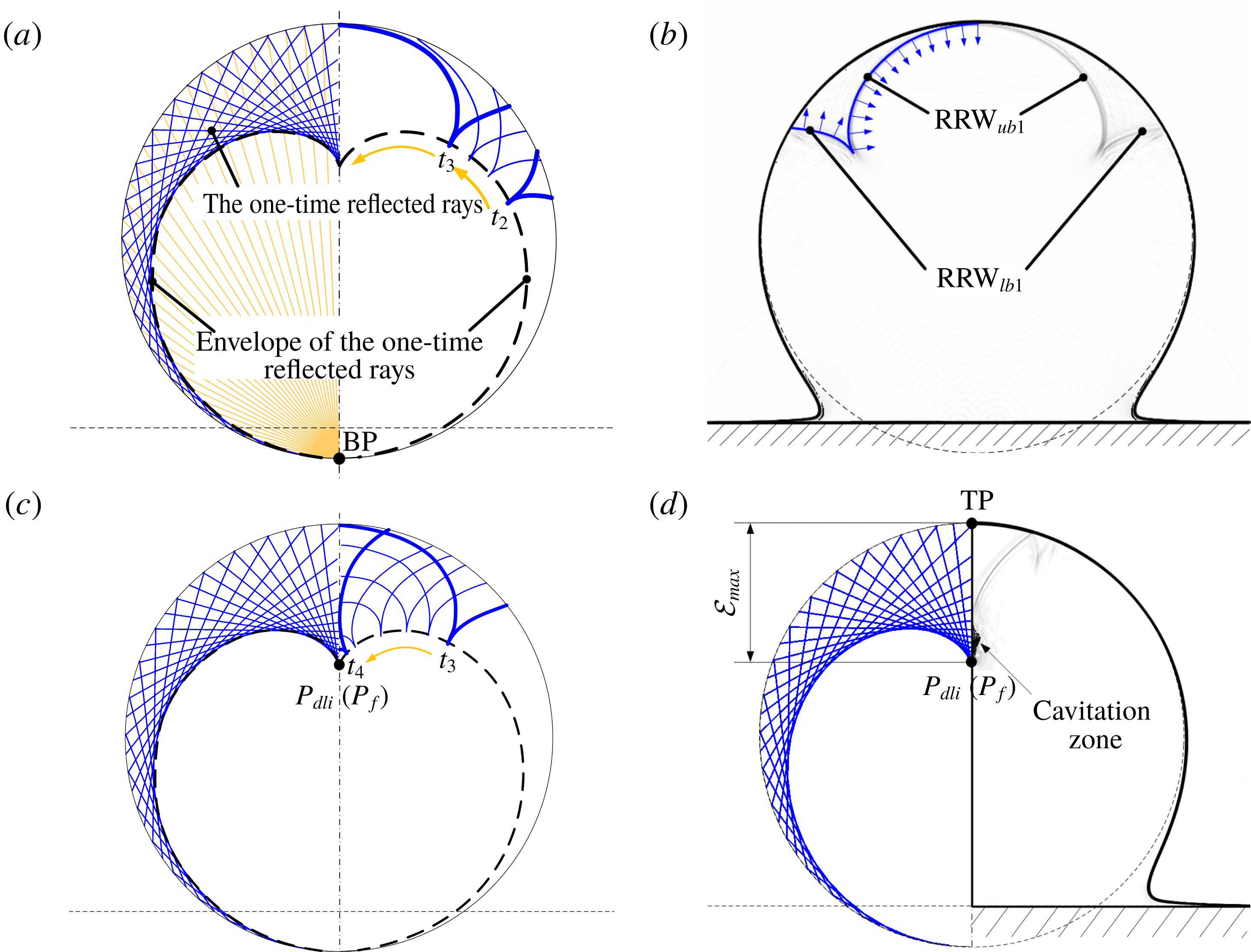
Figure 9. (a) All the first reflected rays emitted from BP with the original angle of the interval
 $[0,\unicode[STIX]{x03C0}/2]$
(a,c), the schematic diagram of the first reflected rarefaction wave propagation from
$[0,\unicode[STIX]{x03C0}/2]$
(a,c), the schematic diagram of the first reflected rarefaction wave propagation from
 $t_{2}(t^{\ast }=0.81)$
to
$t_{2}(t^{\ast }=0.81)$
to
 $t_{3}(t^{\ast }=0.975)$
(b,d). (b) The numerical schlieren contour at
$t_{3}(t^{\ast }=0.975)$
(b,d). (b) The numerical schlieren contour at
 $t^{\ast }=0.975(t_{3})$
. (c) The schematic diagram of the first reflected rarefaction wave propagation from
$t^{\ast }=0.975(t_{3})$
. (c) The schematic diagram of the first reflected rarefaction wave propagation from
 $t_{3}(t^{\ast }=0.975)$
to
$t_{3}(t^{\ast }=0.975)$
to
 $t_{4}(t^{\ast }=1.305)$
. (d) The numerical schlieren contour at
$t_{4}(t^{\ast }=1.305)$
. (d) The numerical schlieren contour at
 $t^{\ast }=1.305(t_{4})$
.
$t^{\ast }=1.305(t_{4})$
.
Five different time instants from time
 $t_{3}$
to
$t_{3}$
to
 $t_{4}$
are chosen to schematically demonstrate the evolution process of
$t_{4}$
are chosen to schematically demonstrate the evolution process of
 $\text{RRW}_{ub1}$
and
$\text{RRW}_{ub1}$
and
 $\text{RRW}_{lb1}$
, figure 9(c). The curvature radius of the arched
$\text{RRW}_{lb1}$
, figure 9(c). The curvature radius of the arched
 $\text{RRW}_{ub1}$
gradually decreases as the reflected rarefaction waves propagate. Finally, the combined arched
$\text{RRW}_{ub1}$
gradually decreases as the reflected rarefaction waves propagate. Finally, the combined arched
 $\text{RRW}_{ub1}$
focuses on the vertical central axis and the focusing point is named
$\text{RRW}_{ub1}$
focuses on the vertical central axis and the focusing point is named
 $P_{f}$
, figure 9(c). Meanwhile, the two following
$P_{f}$
, figure 9(c). Meanwhile, the two following
 $\text{RRW}_{lb1}$
become wider as they propagate upstream. The intersection point of
$\text{RRW}_{lb1}$
become wider as they propagate upstream. The intersection point of
 $\text{RRW}_{ub1}$
and
$\text{RRW}_{ub1}$
and
 $\text{RRW}_{lb1}$
keeps moving along the envelope of the reflected rays with one-time reflection.
$\text{RRW}_{lb1}$
keeps moving along the envelope of the reflected rays with one-time reflection.
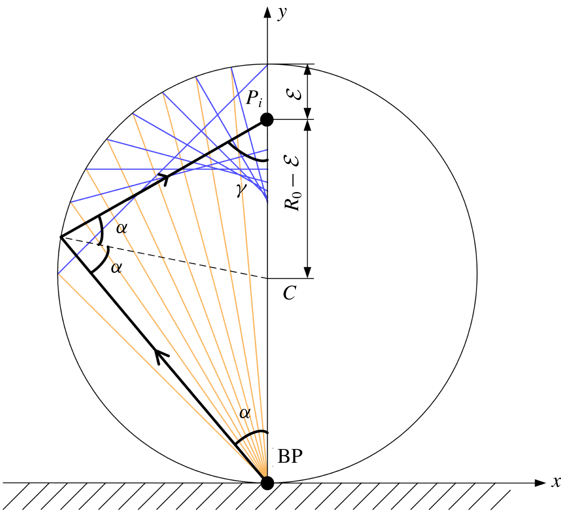
Figure 10. Schematic diagram for the intersection point between the reflected rays, with one-time reflection, and the vertical central axis.
As the one-time reflected rays are related to the propagation of the first reflected rarefaction wave, we can use these one-time reflected rays to analyse the position of
 $P_{f}$
of the arched
$P_{f}$
of the arched
 $\text{RRW}_{ub1}$
. As shown in figure 9(c), the envelope of the one-time reflected rays corresponds to their limiting boundary and the reflected rays are concentrated on their envelope. The concentrated reflected rays represent the superposition of the
$\text{RRW}_{ub1}$
. As shown in figure 9(c), the envelope of the one-time reflected rays corresponds to their limiting boundary and the reflected rays are concentrated on their envelope. The concentrated reflected rays represent the superposition of the
 $\text{RRW}_{ub1}$
and
$\text{RRW}_{ub1}$
and
 $\text{RRW}_{lb1}$
, which is related to the local minimum-pressure region at each time instant, figure 8. The envelopes of the left and right sides interact on the vertical central axis. The intersection point is also the downward limiting position of the one-time reflected rays that intersect with the vertical central axis, and is named the downward limiting intersection point,
$\text{RRW}_{lb1}$
, which is related to the local minimum-pressure region at each time instant, figure 8. The envelopes of the left and right sides interact on the vertical central axis. The intersection point is also the downward limiting position of the one-time reflected rays that intersect with the vertical central axis, and is named the downward limiting intersection point,
 $P_{dli}$
, figure 9(d).
$P_{dli}$
, figure 9(d).
The position of
 $P_{dli}$
can be obtained theoretically according to the ray analysis (Obreschkow et al.
Reference Obreschkow, Dorsaz, Kobel, de Bosset, Tinguely, Field and Farhat2011). Figure 10 shows a series of rays emitted from the BP with the emitting angles
$P_{dli}$
can be obtained theoretically according to the ray analysis (Obreschkow et al.
Reference Obreschkow, Dorsaz, Kobel, de Bosset, Tinguely, Field and Farhat2011). Figure 10 shows a series of rays emitted from the BP with the emitting angles
 $\unicode[STIX]{x1D6FC}$
holding the interval of
$\unicode[STIX]{x1D6FC}$
holding the interval of
 $[0,\unicode[STIX]{x03C0}/4]$
, where the one-time reflected rays can intersect with the vertical central axis. If an arbitrary ray (the black solid lines with an arrow) is chosen, the distance
$[0,\unicode[STIX]{x03C0}/4]$
, where the one-time reflected rays can intersect with the vertical central axis. If an arbitrary ray (the black solid lines with an arrow) is chosen, the distance
 $\unicode[STIX]{x1D6FF}$
between the intersection point
$\unicode[STIX]{x1D6FF}$
between the intersection point
 $P_{i}$
(the intersection point of the first reflected ray with the vertical central axis) and the TP of the column can be expressed as follows:
$P_{i}$
(the intersection point of the first reflected ray with the vertical central axis) and the TP of the column can be expressed as follows:
 $$\begin{eqnarray}\unicode[STIX]{x1D6FF}=R_{0}-\frac{\sin \unicode[STIX]{x1D6FC}\cdot R_{0}}{\sin \unicode[STIX]{x1D6FE}},\end{eqnarray}$$
where
 $R_{0}$
is the initial radius of the water column. The intersection angles
$R_{0}$
is the initial radius of the water column. The intersection angles
 $\unicode[STIX]{x1D6FC}$
and
$\unicode[STIX]{x1D6FC}$
and
 $\unicode[STIX]{x1D6FE}$
are shown in figure 10. The distance
$\unicode[STIX]{x1D6FE}$
are shown in figure 10. The distance
 $\unicode[STIX]{x1D6FF}$
can be rewritten as follows:
$\unicode[STIX]{x1D6FF}$
can be rewritten as follows:
 $$\begin{eqnarray}\unicode[STIX]{x1D6FF}=R_{0}-\frac{R_{0}}{3-4\sin ^{2}\unicode[STIX]{x1D6FC}},\end{eqnarray}$$
where
 $\unicode[STIX]{x1D6FC}\in [0,\unicode[STIX]{x03C0}/4]$
. A maximum limiting value of
$\unicode[STIX]{x1D6FC}\in [0,\unicode[STIX]{x03C0}/4]$
. A maximum limiting value of
 $\unicode[STIX]{x1D6FF}$
exists, thus, the position of
$\unicode[STIX]{x1D6FF}$
exists, thus, the position of
 $P_{dli}$
of the one-time reflected rays is obtained, which has the following expression:
$P_{dli}$
of the one-time reflected rays is obtained, which has the following expression:
 $$\begin{eqnarray}\unicode[STIX]{x1D6FF}_{max}=\lim _{\unicode[STIX]{x1D6FC}\rightarrow 0}\left(R_{0}-\frac{R_{0}}{3-4\sin ^{2}\unicode[STIX]{x1D6FC}}\right)=\frac{2}{3}R_{0}=\frac{D_{0}}{3},\end{eqnarray}$$
where
 $D_{0}$
is the initial diameter of the water column.
$D_{0}$
is the initial diameter of the water column.
The above expression for determining the position of
 $P_{dli}$
corresponds to the rays initially emitted from one contact point (i.e. from one wavelet). We observed that
$P_{dli}$
corresponds to the rays initially emitted from one contact point (i.e. from one wavelet). We observed that
 $P_{dli}$
overlaps with
$P_{dli}$
overlaps with
 $P_{f}$
, which indicates that
$P_{f}$
, which indicates that
 $\text{RRW}_{ub1}$
finally focuses at a position
$\text{RRW}_{ub1}$
finally focuses at a position
 $1/3$
of the droplet diameter away from TP, figure 9(c). In fact, there are an infinite number of emitted wavelets forming the shock envelope before the critical time
$1/3$
of the droplet diameter away from TP, figure 9(c). In fact, there are an infinite number of emitted wavelets forming the shock envelope before the critical time
 $t_{c}$
. They also focus on the same limiting intersection point (
$t_{c}$
. They also focus on the same limiting intersection point (
 $P_{dli}$
) at the same time instant, based on a similar analysis of the emitted ray, however, they are not shown here. In another aspect, the arched
$P_{dli}$
) at the same time instant, based on a similar analysis of the emitted ray, however, they are not shown here. In another aspect, the arched
 $\text{RRW}_{ub1}$
that corresponds to the infinite reflected rays at each time instant, the focusing point of these infinite rays and the
$\text{RRW}_{ub1}$
that corresponds to the infinite reflected rays at each time instant, the focusing point of these infinite rays and the
 $P_{f}$
that corresponds to
$P_{f}$
that corresponds to
 $\text{RRW}_{ub1}$
, are consistent.
$\text{RRW}_{ub1}$
, are consistent.
Due to the focusing effect of the reflected rarefaction waves, a local low-pressure zone is created in the stretched liquid. Therefore, the pressure around
 $P_{f}$
is significantly lowered and reaches a value below the
$P_{f}$
is significantly lowered and reaches a value below the
 $p_{threshold}$
, which means that the transient phase-transition process is triggered, and cavitation occurs. Subsequently, the cavity will grow to be a visible cavitation zone. The predicted position of
$p_{threshold}$
, which means that the transient phase-transition process is triggered, and cavitation occurs. Subsequently, the cavity will grow to be a visible cavitation zone. The predicted position of
 $P_{f}$
fits well with that of the observations, both in the experimental and numerical results, figures 5(j) and 9(d).
$P_{f}$
fits well with that of the observations, both in the experimental and numerical results, figures 5(j) and 9(d).
So far, we have analysed the spatio-temporal evolution of the confined shock and the first reflected rarefaction wave before
 $\text{RRW}_{ub1}$
focuses on the vertical central axis. Subsequently, the complicated multi-reflected waves and the cavity collapse inside the droplet will appear. We will try to elaborate on these further in this section.
$\text{RRW}_{ub1}$
focuses on the vertical central axis. Subsequently, the complicated multi-reflected waves and the cavity collapse inside the droplet will appear. We will try to elaborate on these further in this section.
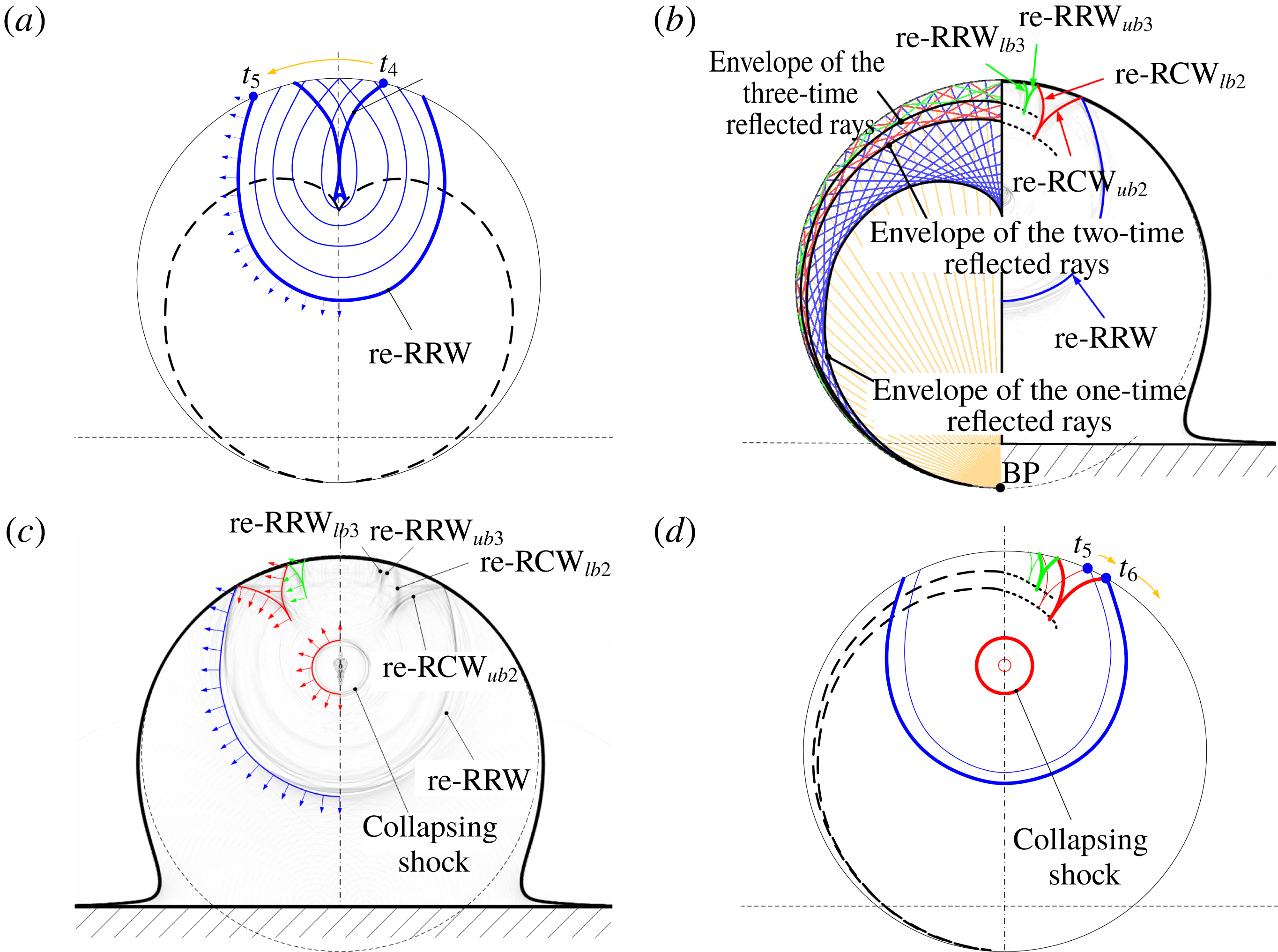
Figure 11. (a) Schematic diagram of the first reflected rarefaction wave propagation from
 $t_{4}$
(
$t_{4}$
(
 $t^{\ast }=1.305$
) to
$t^{\ast }=1.305$
) to
 $t_{5}$
(
$t_{5}$
(
 $t^{\ast }=1.545$
). (b) All of the emitted rays from BP with one-, two- and three-time reflection with the original angle of the interval [
$t^{\ast }=1.545$
). (b) All of the emitted rays from BP with one-, two- and three-time reflection with the original angle of the interval [
 $0,\unicode[STIX]{x03C0}/2$
] (a,c), and the numerical schlieren contour at time
$0,\unicode[STIX]{x03C0}/2$
] (a,c), and the numerical schlieren contour at time
 $t_{5}$
(
$t_{5}$
(
 $t^{\ast }=1.545$
) (b,d). (c) Numerical schlieren contour at time
$t^{\ast }=1.545$
) (b,d). (c) Numerical schlieren contour at time
 $t_{6}$
(
$t_{6}$
(
 $t^{\ast }=1.59$
). (d) Schematic diagram of the reflected waves’ propagation from
$t^{\ast }=1.59$
). (d) Schematic diagram of the reflected waves’ propagation from
 $t_{5}$
(
$t_{5}$
(
 $t^{\ast }=1.545$
) to
$t^{\ast }=1.545$
) to
 $t_{6}$
(
$t_{6}$
(
 $t^{\ast }=1.59$
).
$t^{\ast }=1.59$
).
Six typical time instants from
 $t_{4}$
to
$t_{4}$
to
 $t_{5}$
are chosen to demonstrate the evolution of the
$t_{5}$
are chosen to demonstrate the evolution of the
 $\text{RRW}_{lb1}$
, figure 11(a). The two branches of symmetrical
$\text{RRW}_{lb1}$
, figure 11(a). The two branches of symmetrical
 $\text{RRW}_{lb1}$
, from the left and right sides, will interact with each other and be reflected at the vertical central axis. After the interaction among the left reflected
$\text{RRW}_{lb1}$
, from the left and right sides, will interact with each other and be reflected at the vertical central axis. After the interaction among the left reflected
 $\text{RRW}_{lb1}$
, the right reflected
$\text{RRW}_{lb1}$
, the right reflected
 $\text{RRW}_{lb1}$
and the re-expanding wave from the focusing point, an expanding re-reflected rarefaction wave (re-RRW) is formed. The shape and position of the re-RRW at
$\text{RRW}_{lb1}$
and the re-expanding wave from the focusing point, an expanding re-reflected rarefaction wave (re-RRW) is formed. The shape and position of the re-RRW at
 $t^{\ast }=1.545\;(t_{5})$
are shown in the numerical schlieren contour, figure 11(b). Two other waves are also observed, which are the second reflected compression wave and the third reflected rarefaction wave, respectively. The peak-pressure value induced by the second reflected waves (compression waves) is
$t^{\ast }=1.545\;(t_{5})$
are shown in the numerical schlieren contour, figure 11(b). Two other waves are also observed, which are the second reflected compression wave and the third reflected rarefaction wave, respectively. The peak-pressure value induced by the second reflected waves (compression waves) is
 $6.31\times 10^{7}~\text{Pa}$
, which is approximately 33 % of
$6.31\times 10^{7}~\text{Pa}$
, which is approximately 33 % of
 $p_{h}$
. The peak-pressure value induced by the third reflected waves (rarefaction waves) is
$p_{h}$
. The peak-pressure value induced by the third reflected waves (rarefaction waves) is
 $-3.0\times 10^{7}~\text{Pa}$
, whose absolute value is approximately 16 % of the value of
$-3.0\times 10^{7}~\text{Pa}$
, whose absolute value is approximately 16 % of the value of
 $p_{h}$
. Therefore, the strength of the reflected waves decreases gradually due to multiple reflections. As shown in figure 11, the repeated reflection waves cannot be clearly observed since they are much weaker. The
$p_{h}$
. Therefore, the strength of the reflected waves decreases gradually due to multiple reflections. As shown in figure 11, the repeated reflection waves cannot be clearly observed since they are much weaker. The
 $\text{RCW}_{ub2}$
,
$\text{RCW}_{ub2}$
,
 $\text{RCW}_{lb2}$
,
$\text{RCW}_{lb2}$
,
 $\text{RRW}_{ub3}$
and
$\text{RRW}_{ub3}$
and
 $\text{RRW}_{lb3}$
propagating from the left and right sides interact with each other and reflect on the vertical central axis. These reflected waves are denoted as re-
$\text{RRW}_{lb3}$
propagating from the left and right sides interact with each other and reflect on the vertical central axis. These reflected waves are denoted as re-
 $\text{RCW}_{ub2}$
, re-
$\text{RCW}_{ub2}$
, re-
 $\text{RCW}_{lb2}$
, re-
$\text{RCW}_{lb2}$
, re-
 $\text{RRW}_{ub3}$
and re-
$\text{RRW}_{ub3}$
and re-
 $\text{RRW}_{lb3}$
, respectively. The reflected wave structures are clearly presented in the numerical schlieren contour, figure 11. The upper concave re-RRW expands towards the bottom wall and is followed by the second and third reflected waves at the end. The intersection points of the upper and lower branches of the second and third reflected waves are moving along the envelopes extracted from the ray analysis, figure 11(d). Three curves related to the envelopes are presented, including the lower, middle and upper branches, figure 11(b). They represent the trajectories of the intersection points of the upper and lower branches of the first, second and third reflected waves, respectively.
$\text{RRW}_{lb3}$
, respectively. The reflected wave structures are clearly presented in the numerical schlieren contour, figure 11. The upper concave re-RRW expands towards the bottom wall and is followed by the second and third reflected waves at the end. The intersection points of the upper and lower branches of the second and third reflected waves are moving along the envelopes extracted from the ray analysis, figure 11(d). Three curves related to the envelopes are presented, including the lower, middle and upper branches, figure 11(b). They represent the trajectories of the intersection points of the upper and lower branches of the first, second and third reflected waves, respectively.
As the re-RRW propagates outward, the cavity caused by the focusing of
 $\text{RRW}_{ub1}$
collapses. The peak pressure during the collapsing of the cavity reaches 81 MPa, which is about 800 times the initial ambient pressure for the present case (initial impaction speed
$\text{RRW}_{ub1}$
collapses. The peak pressure during the collapsing of the cavity reaches 81 MPa, which is about 800 times the initial ambient pressure for the present case (initial impaction speed
 $V_{0}=110~\text{m}~\text{s}^{-1}$
). From the numerical schlieren contours shown in figure 11(b,c), a circular shock wave, which is known as the collapsing shock, is found as the cavity collapses and explodes outwards. Finally, the collapsing shock will reach the bottom wall, the results at this time are not shown, and potentially damage it.
$V_{0}=110~\text{m}~\text{s}^{-1}$
). From the numerical schlieren contours shown in figure 11(b,c), a circular shock wave, which is known as the collapsing shock, is found as the cavity collapses and explodes outwards. Finally, the collapsing shock will reach the bottom wall, the results at this time are not shown, and potentially damage it.
To summarize, combining numerical simulation with theoretical approximation, the unsteady wave structures (including the confined shock, the multi-reflected waves and the cavitation collapsing shock), inside the droplet during the impingement of a high-speed cylindrical droplet on a solid wall are carefully analysed. The properties of the waves and their evolution processes inside the droplet are elucidated with the help of the ray analysis, which, to the authors’ knowledge, are not clarified in the previously available literatures.
5 Effects of impaction speed
In this section, different initial impaction speeds, 50, 110, 150 and
 $200~\text{m}~\text{s}^{-1}$
, are considered for the water column impaction on a solid wall.
$200~\text{m}~\text{s}^{-1}$
, are considered for the water column impaction on a solid wall.
Both the analytical (calculated by (4.1)) and numerical values of the critical angle,
 $\unicode[STIX]{x1D703}_{c}$
, under the different impaction speeds are shown in table 2;
$\unicode[STIX]{x1D703}_{c}$
, under the different impaction speeds are shown in table 2;
 $\unicode[STIX]{x1D703}_{c}$
increases with the increase of the initial impaction speed. The temporal variations of the characteristic scales, including the length
$\unicode[STIX]{x1D703}_{c}$
increases with the increase of the initial impaction speed. The temporal variations of the characteristic scales, including the length
 $d_{l}$
and width
$d_{l}$
and width
 $d_{w}$
, of the water column, figure 12, are normalized by the initial column diameter;
$d_{w}$
, of the water column, figure 12, are normalized by the initial column diameter;
 $d_{l}$
is defined as the distance from the wall to TP and
$d_{l}$
is defined as the distance from the wall to TP and
 $d_{w}$
is defined as the diameter along the centre of the column in the horizontal direction. It is observed that
$d_{w}$
is defined as the diameter along the centre of the column in the horizontal direction. It is observed that
 $d_{l}$
of the column decreases, while
$d_{l}$
of the column decreases, while
 $d_{w}$
increases, with time as the water column impacts on the wall. The decreasing rate of
$d_{w}$
increases, with time as the water column impacts on the wall. The decreasing rate of
 $d_{l}$
is larger for higher initial impaction speed. At
$d_{l}$
is larger for higher initial impaction speed. At
 $t^{\ast }=1$
the curve has a turning point for each chosen impaction speed, figure 12(a). This is the exact time when the confined shock arrives at the TP of the column. The width of the column keeps unchanged until
$t^{\ast }=1$
the curve has a turning point for each chosen impaction speed, figure 12(a). This is the exact time when the confined shock arrives at the TP of the column. The width of the column keeps unchanged until
 $t^{\ast }=0.6$
, then it increases rapidly for all the chosen impaction speeds, as shown in figure 12(b).
$t^{\ast }=0.6$
, then it increases rapidly for all the chosen impaction speeds, as shown in figure 12(b).
Table 2. The analytical and numerical
 $\unicode[STIX]{x1D703}_{c}$
for different initial impaction speeds.
$\unicode[STIX]{x1D703}_{c}$
for different initial impaction speeds.

Figure 12. The time evolution of the dimensionless length (a) and width (b) of the water column.
The pressure distributions along the vertical central line for the different cases that non-dimensionalized by each corresponding water hammer pressure
 $p_{h}$
(calculated by (4.3)) at the dimensionless times of
$p_{h}$
(calculated by (4.3)) at the dimensionless times of
 $t^{\ast }=0.45$
and
$t^{\ast }=0.45$
and
 $t^{\ast }=0.9$
are shown in figure 13. It is found that the confined shock wave will be strengthened with a higher initial impaction speed, as the pressure behind the confined shock wave is much larger for higher impaction speeds. It is shown that the strength of the confined shock wave gradually decreases along its propagation. Through the comparison of pressure distributions non-dimensionalized by
$t^{\ast }=0.9$
are shown in figure 13. It is found that the confined shock wave will be strengthened with a higher initial impaction speed, as the pressure behind the confined shock wave is much larger for higher impaction speeds. It is shown that the strength of the confined shock wave gradually decreases along its propagation. Through the comparison of pressure distributions non-dimensionalized by
 $p_{h}$
, it is shown that the weaker the intensity of the shock wave, the more the pressure decays at the same dimensionless instant. Furthermore, for higher impaction speeds, the stronger confined shock wave will reflect off the column surface like to the reflected rarefaction waves. Therefore, the convergence region will be larger for higher impaction speeds.
$p_{h}$
, it is shown that the weaker the intensity of the shock wave, the more the pressure decays at the same dimensionless instant. Furthermore, for higher impaction speeds, the stronger confined shock wave will reflect off the column surface like to the reflected rarefaction waves. Therefore, the convergence region will be larger for higher impaction speeds.

Figure 13. Dimensionless pressure value along the vertical central line for the four simulation cases at time instants
 $t^{\ast }=0.45$
(a) and
$t^{\ast }=0.45$
(a) and
 $t^{\ast }=0.9$
(b).
$t^{\ast }=0.9$
(b).
Consequently, figure 14 shows the pressure contours at the time when the first reflected waves converge for the different impaction speeds. This also corresponds to the time when cavitation occurs, in which the cavitation zone is marked by the isoline of the vapour volume fraction. The impaction speed is equal to, or larger than,
 $110~\text{m}~\text{s}^{-1}$
, among the present four chosen speeds, and the convergence of the rarefaction waves can induce the cavitation since the local pressure is below
$110~\text{m}~\text{s}^{-1}$
, among the present four chosen speeds, and the convergence of the rarefaction waves can induce the cavitation since the local pressure is below
 $p_{threshold}$
, figure 15(a), which presents the dimensionless pressure distributions. The cavitation zone becomes larger as the impaction speed increases from
$p_{threshold}$
, figure 15(a), which presents the dimensionless pressure distributions. The cavitation zone becomes larger as the impaction speed increases from
 $110$
to
$110$
to
 $200~\text{m}~\text{s}^{-1}$
.
$200~\text{m}~\text{s}^{-1}$
.

Figure 14. Pressure contours when the reflected waves come to focus for different impaction speeds. The time instant is
 $t^{\ast }=1.275$
, 1.305, 1.305 and 1.335, corresponding to the initial impaction speeds of 50, 110, 150 and
$t^{\ast }=1.275$
, 1.305, 1.305 and 1.335, corresponding to the initial impaction speeds of 50, 110, 150 and
 $200~\text{m}~\text{s}^{-1}$
, respectively. For (b–d) the time also relates to that when the maximum cavitation zone occurs. The white solid line represents the isoline of the vapour volume fraction.
$200~\text{m}~\text{s}^{-1}$
, respectively. For (b–d) the time also relates to that when the maximum cavitation zone occurs. The white solid line represents the isoline of the vapour volume fraction.
Referring to the distributions of the vapour volume fraction, along the vertical central lines, for the four chosen impaction speeds, figure 15(b), the vapour volume fraction rises sharply in the cavitation region and is located between
 $y/D_{0}=0.45$
and 0.7 for
$y/D_{0}=0.45$
and 0.7 for
 $V_{0}=110$
, 150 and
$V_{0}=110$
, 150 and
 $200~\text{m}~\text{s}^{-1}$
. The profiles of the vapour volume fraction also indicate that the cavitation zone becomes larger for higher impaction speeds ranging from
$200~\text{m}~\text{s}^{-1}$
. The profiles of the vapour volume fraction also indicate that the cavitation zone becomes larger for higher impaction speeds ranging from
 $110$
to
$110$
to
 $200~\text{m}~\text{s}^{-1}$
.
$200~\text{m}~\text{s}^{-1}$
.

Figure 15. Dimensionless pressure (a) and vapour volume fraction (b) along the vertical central axis for different initial speeds at the times of
 $t^{\ast }=1.275$
, 1.305, 1.305 and 1.335, respectively, which refer to the contours in figure 14.
$t^{\ast }=1.275$
, 1.305, 1.305 and 1.335, respectively, which refer to the contours in figure 14.
Figure 16 shows the pressure contours at the moment the cavity (if there is any) collapses completely and shock waves are emitted. In the case of
 $V_{0}=50~\text{m}~\text{s}^{-1}$
, no cavitation is observed, and the reflected rarefaction wave propagates upstream, figure 16(a). As shown in figure 16, stronger collapsing waves can be induced by stronger impaction and they need a longer time to collapse. Very complicated structures involving reflected waves, the circular collapsing shock wave and refraction waves evolve inside the column.
$V_{0}=50~\text{m}~\text{s}^{-1}$
, no cavitation is observed, and the reflected rarefaction wave propagates upstream, figure 16(a). As shown in figure 16, stronger collapsing waves can be induced by stronger impaction and they need a longer time to collapse. Very complicated structures involving reflected waves, the circular collapsing shock wave and refraction waves evolve inside the column.
In a later stage, a splash will occur for the impacted high-speed droplet, but this is beyond the present research. The contact line dynamics is dominated by the inertial effects of the droplet in the earlier stages of impaction, which occurs irrespective of the physical properties of the liquid and the surface, and the wettability is also not influential (Yarin Reference Yarin2005). Therefore, the analysis of contact line dynamics is also not considered in the present study.
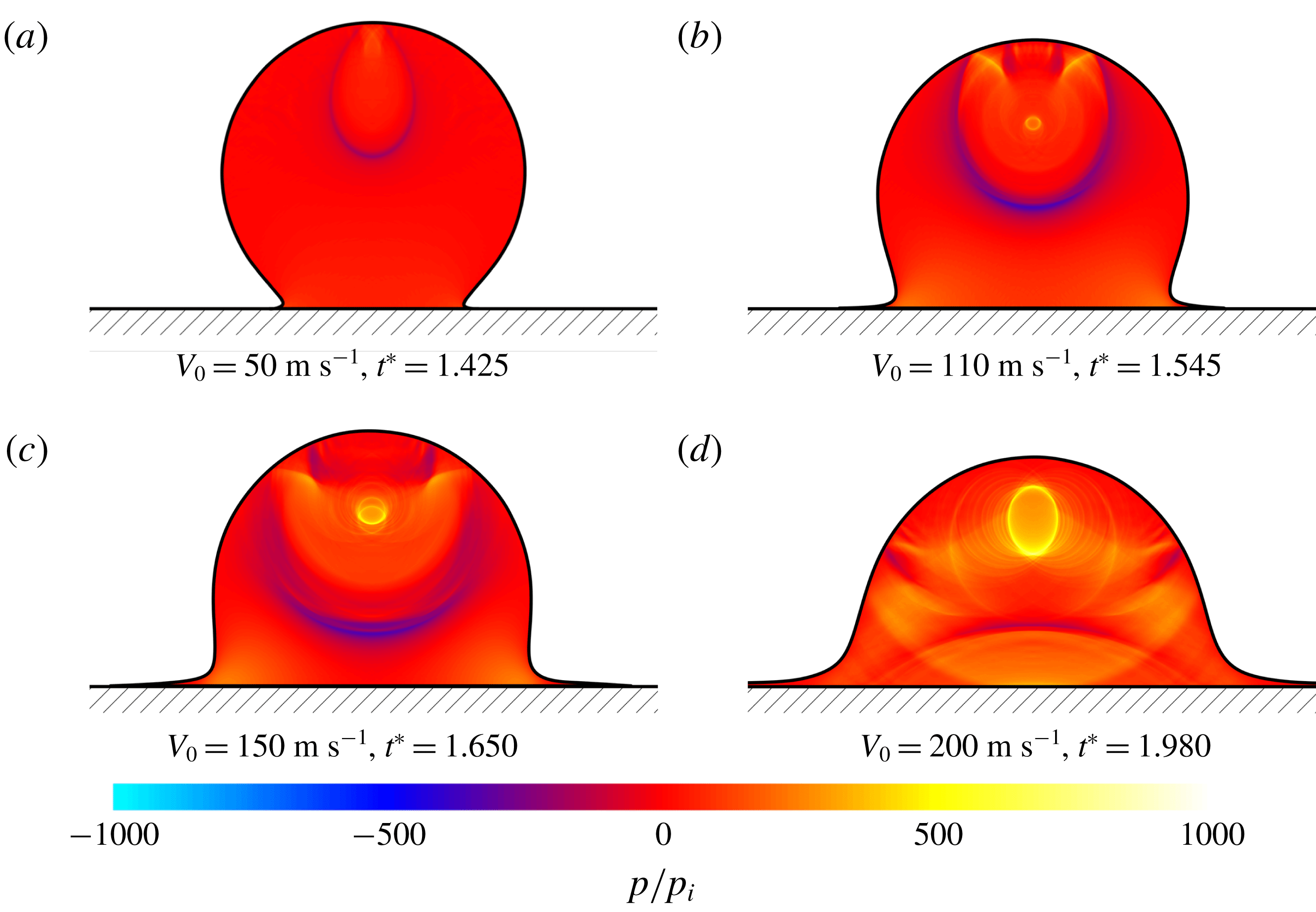
Figure 16. Pressure contours at the time the cavities collapse. The time instant is
 $t^{\ast }=1.425$
, 1.545, 1.650 and 1.980, corresponding to the initial impaction speeds of 50, 110, 150 and
$t^{\ast }=1.425$
, 1.545, 1.650 and 1.980, corresponding to the initial impaction speeds of 50, 110, 150 and
 $200~\text{m}~\text{s}^{-1}$
, respectively. The shock waves emitted from the collapsing bubble are visible for the cases of
$200~\text{m}~\text{s}^{-1}$
, respectively. The shock waves emitted from the collapsing bubble are visible for the cases of
 $V_{0}=110$
, 150 and
$V_{0}=110$
, 150 and
 $200~\text{m}~\text{s}^{-1}$
.
$200~\text{m}~\text{s}^{-1}$
.
6 Conclusion and remarks
This study involved a numerical investigation of high-speed cylindrical droplet impingement on a solid wall, and also contributed to the improvement of the phase-transition model and algorithm for the highly compressible two-phase flows. More specifically, the promoted two-phase multi-component compressible fluid model, coupled with a phase-transition model describing the homogeneous cavitation process, is used to describe the Eulerian flow system. The phase transition is triggered in the simulation when the local fluid pressure is lower than the threshold value. This is justified by the pressure–temperature expression obtained from the linear approximation of the curve for the cavitation pressure. The numerical chemical potential relaxation process is employed to decouple the solution of the source terms with a hyperbolic operator. Thus, the cavitation evolution process inside the droplet can be captured in detail, which has not been presented in previous work. The analyses of the physical mechanism, such as the generation and propagation of complex wave structures, and the inception and collapsing of the cavity, are then conducted based on the simulation results.
The simulation of the impingement of a
 $110~\text{m}~\text{s}^{-1}$
water column on a solid wall reproduced the cavitation inception observed in the experiments and the evolution process of the collapsing of the cavitation zones. A detailed analysis was presented for the above process showing the evolution and interaction of the complicated waves inside the column. The confined shock wave is generated immediately after the impingement of the water column on the wall and it propagates inside the water column. When the contact angle
$110~\text{m}~\text{s}^{-1}$
water column on a solid wall reproduced the cavitation inception observed in the experiments and the evolution process of the collapsing of the cavitation zones. A detailed analysis was presented for the above process showing the evolution and interaction of the complicated waves inside the column. The confined shock wave is generated immediately after the impingement of the water column on the wall and it propagates inside the water column. When the contact angle
 $\unicode[STIX]{x1D703}$
is larger than the critical value, the confined shock wave will detach from the solid wall and continually propagate towards the top surface of the column. Meanwhile, the confined shock wave will be reflected by the surface of the liquid column and generate a series of rarefaction waves. The convergence of the rarefaction waves can induce low-pressure regions. Those regions interact and gradually merge at the vertical axis, the position of which is located at approximately one third of the initial diameter away from the top pole. The local fluid state reaches the thermodynamic threshold condition for triggering of the phase transition and cavitation occurs. The capture of the inception of cavitation by the present numerical simulation is consistent with that observed in the experiments. Furthermore, the evolution process of the cavitation zone, including the development and collapse, is further discussed. Once the cavity collapses, a series of shock waves is emitted, which again increase the pressure of the local fluid.
$\unicode[STIX]{x1D703}$
is larger than the critical value, the confined shock wave will detach from the solid wall and continually propagate towards the top surface of the column. Meanwhile, the confined shock wave will be reflected by the surface of the liquid column and generate a series of rarefaction waves. The convergence of the rarefaction waves can induce low-pressure regions. Those regions interact and gradually merge at the vertical axis, the position of which is located at approximately one third of the initial diameter away from the top pole. The local fluid state reaches the thermodynamic threshold condition for triggering of the phase transition and cavitation occurs. The capture of the inception of cavitation by the present numerical simulation is consistent with that observed in the experiments. Furthermore, the evolution process of the cavitation zone, including the development and collapse, is further discussed. Once the cavity collapses, a series of shock waves is emitted, which again increase the pressure of the local fluid.
The effects of different initial impaction speeds on droplet dynamics and cavitation structures were investigated. The initial impact speed was chosen as 50, 110, 150 and
 $200~\text{m}~\text{s}^{-1}$
respectively. The numerical results showed that the impaction speed has a significant influence on the strength of the confined shock wave, which increases with the impaction speed. For a higher initial speed, the critical contact angle
$200~\text{m}~\text{s}^{-1}$
respectively. The numerical results showed that the impaction speed has a significant influence on the strength of the confined shock wave, which increases with the impaction speed. For a higher initial speed, the critical contact angle
 $\unicode[STIX]{x1D703}_{c}$
is larger, and a larger cavitation zone is induced. Larger cavitation zones and stronger collapsing waves are recognized for higher initial impaction speeds. The geometrical morphology of the droplet is abstracted by analysing the two-phase interface structures.
$\unicode[STIX]{x1D703}_{c}$
is larger, and a larger cavitation zone is induced. Larger cavitation zones and stronger collapsing waves are recognized for higher initial impaction speeds. The geometrical morphology of the droplet is abstracted by analysing the two-phase interface structures.
In this study, a conserved Eulerian system was employed. However, even though the viscosity and surface tension can be both neglected in a high-speed impaction process, their effect on the cavitation and collapse should be taken into account, separately or jointly, in the future. Furthermore, the extension studies should be carried out for droplets of different liquids.
Acknowledgements
The authors would like to acknowledge partial financial support from the Natural Science Foundation of China (nos 51676111, 11628206 and NSAF-U1730104), the State Key Laboratory of Chemical Engineering (no. SKL-ChE-16A02) and the Tsinghua University Initiative Scientific Research Program.