


1. Introduction
The mechanism of boundary layer transition is one of the most active research fields in contemporary fluid dynamics, not only because of its complexity in mathematics and physics, but also for the enormous potential applications in practical engineering. Over the years, linear stability theory (LST) has played an essential role in revealing the mechanisms of flow instability. Moreover, by using LST, some of the fundamental mechanisms are now well understood. Representative examples are Tollmien–Schlichting (TS) waves (Schlichting & Gersten Reference Schlichting and Gersten2017), Mack modes (Mack Reference Mack1975) and cross-flow modes (Saric, Reed & White Reference Saric, Reed and White2003) in two- and three-dimensional boundary layers. More detailed works in this field could be found in reviews by Reed & Saric (Reference Reed and Saric1989), Reed, Saric & Arnal (Reference Reed, Saric and Arnal1996), Fedorov (Reference Fedorov2011) and Zhong & Wang (Reference Zhong and Wang2012). However, owing to the richness of flow physics in high-speed flows, flow instability is still far from fully understood, even in terms of fundamental modal instability.
In particular, the leading edge of a wing plays a very important role in boundary layer transition. One noticeable phenomenon in experiments (Pfenninger Reference Pfenninger1965) is the leading-edge contamination: if the Reynolds number is sufficiently high, initial turbulent flow could persist along the attachment line. In real flight vehicles, owing to significant geometric variation in wing–body junctions, initial laminar flow could easily become turbulent, contaminating the flow state of the attachment line. Such phenomenon motivated the discovery of the mechanism of the attachment-line transition.
The steady laminar flow in the leading-edge region of a swept wing was often studied using the Hiemenz model (Rosenhead Reference Rosenhead1963). Unlike the similarity solution for conventional boundary layer flows, the Hiemenz model provides an exact solution of incompressible Navier–Stokes (NS) equations in the leading edge. The agreement with the experimentally measured basic flow (Gaster Reference Gaster1967) further popularized the Hiemenz model. Poll (Reference Poll1979) performed experiments over a swept cylinder, the preliminary measurements of the velocity profile along the attachment-line was in good agreement with those predicted by the Hiemenz model. In addition, he was the first to establish a distinction between the transition induced by cross-flow and transition initiated by attachment-line instabilities.
The first theoretical stability study of the attachment-line boundary layer was given by Hall, Malik & Poll (Reference Hall, Malik and Poll1984) in the temporal framework. Under the assumption made by Görtler (Reference Görtler1955) and Hämmerlin, Görtler & Tollmien (Reference Hämmerlin, Görtler and Tollmien1955) for Hiemenz flow (the linear instability in the attachment-line acquires the symmetry of the basic flow, in which chordwise velocity is a linear function of the chordwise coordinate), they demonstrated that this flow is linearly unstable to travelling wave disturbances that propagate along the attachment line. Later, Theofilis (Reference Theofilis1995) performed linear stability analysis of incompressible attachment-line flow in the spatial framework and the continuous spectrum was analysed with asymptotic theory. A more comprehensive stability study was later given by Theofilis (Reference Theofilis1998) and, in this paper, all linear approaches (local temporal/spatial linear analyses) utilized to that time are used, together with the nonlinear numerical simulations, to cover the linear and nonlinear features. Subsequently, Lin & Malik (Reference Lin and Malik1996) discarded the Görtler–Hämmerlin (G–H) assumption and directly solved partial differential eigenvalue problems based on the Hiemenz model. They uncovered a series of symmetric and antisymmetric discrete modes and found the symmetric modes always have larger growth rate. They also found a stabilizing effect of the leading-edge curvature (Lin & Malik Reference Lin and Malik1997). An extension of the G–H model for an attachment-line boundary layer is given by Theofilis et al. (Reference Theofilis, Fedorov, Obrist and Dallmann2003): this extension permits recasting the partial differential eigenvalue problem as a sequence of ordinary differential eigenvalue problems which govern the two families of symmetric and antisymmetric instabilities. At the same time, Obrist & Schmid (Reference Obrist and Schmid2003a) provided a complete analysis of the temporal spectrum using Hermite expansions along the chordwise direction. Then, they performed the analysis of non-model effects and receptivity of this problem (Obrist & Schmid Reference Obrist and Schmid2003b). On the aspect of direct numerical simulations (DNS), Spalart (Reference Spalart1988) confirmed that the leading unstable mode satisfied the G–H assumption for Hiemenz flows. Joslin (Reference Joslin1995) also performed DNS and found the stabilizing effect of surface suction on attachment-line modes.
In compressible flows, early stability properties of subsonic leading-edge boundary layer flow were discussed by Theofilis, Fedorov & Collis (Reference Theofilis, Fedorov and Collis2006). In their work, the problem was solved both numerically and theoretically. They demonstrated that the three-dimensional polynomial eigenmodes of an incompressible flow (Theofilis et al. Reference Theofilis, Fedorov, Obrist and Dallmann2003) persisted in the subsonic flow regime. Later, a more accurate analogy analysis based on sparse techniques was performed by Gennaro et al. (Reference Gennaro, Rodríguez, Medeiros and Theofilis2013). Their results perfectly matched those from theoretical analysis over a large parameter range in the subsonic region. They found that when the sweep Mach number decreased, the range of the unstable region and the growth rates became larger, but the critical Reynolds numbers increased.
As the free-stream Mach number further increases from subsonic to supersonic, the compressibility effects become more significant. The investigation of supersonic attachment-line flow was initially focused on the influence of sweep angles and the heat flux along the attachment line (Gallagher & Beckwith Reference Gallagher and Beckwith1959). The transition of the attachment-line flow was also detected by Gallagher & Beckwith (Reference Gallagher and Beckwith1959). In their Mach 4.15 experimental study, the effect of sweep angles was studied in a relatively large range. Later, Creel, Beckwith & Chen (Reference Creel, Beckwith and Chen1986) performed experiments with a free-stream Mach number of 3.5 and several sweep angles. They detected transition along the attachment line and found the transition Reynolds numbers to be around 650 (based on boundary layer length scale at the leading edge). Skuratov & Fedorov (Reference Skuratov and Fedorov1991) performed a similar test to validate the results of Creel et al. (Reference Creel, Beckwith and Chen1986). Murakami, Stanewsky & Krogmann (Reference Murakami, Stanewsky and Krogmann1996) conducted experiments on hypersonic attachment-line flow in a Ludwieg-tube wind tunnel. They found that the critical Reynolds number increased slightly as the sweep Mach number increased. Gaillard, Benard & Alziary de Roquefort (Reference Gaillard, Benard and Alziary de Roquefort1999) presented extensive experimental results for hypersonic attachment-line flow with various sweep Mach numbers. It is interesting to note that the critical Reynolds number decreased as the sweep Mach number was above 5.
Apart from experimental studies, researchers also tried to understand the Mach number effect theoretically. An early theoretical attempt to study the stability of compressible attachment line was made by Malik & Beckwith (Reference Malik and Beckwith1988) with perturbations of TS type. However, this assumption neglected the chordwise dependence of the basic flow. A more proper assumption was made later by Lin & Malik (Reference Lin and Malik1995), where two-dimensional eigenvalue problems were solved directly, allowing two-dimensional dependence of the mean flow in the solution. It was found that the attachment-line flow was subject to three-dimensional instability. In addition, the critical Reynolds number based on the momentum thickness was found to be around 125. Semisynov et al. (Reference Semisynov, Fedorov, Novikov, Semionov and Kosinov2003) performed a combined theoretical and experimental study and found the critical transition Reynolds numbers were higher in supersonic than in subsonic flows. More recently, Mack et al. published a series of studies (Mack, Schmid & Sesterhenn Reference Mack, Schmid and Sesterhenn2008; Mack & Schmid Reference Mack and Schmid2010a, Reference Mack and Schmid2011a,Reference Mack and Schmidb) focusing on hypersonic flows around a yawed parabolic body of infinite span with their innovative Jacobi-free global stability solver (Mack & Schmid Reference Mack and Schmid2010b). The global spectrum that contained both attachment-line and cross-flow instabilities was presented for a sweep Mach number of 1.25. Some modes were found to reflect features of both attachment-line and cross-flow instabilities. They also observed that the unstable acoustic mode could coexist with the unstable boundary mode. The relative critical Reynolds number of the most unstable acoustic mode was smaller than the unstable boundary mode.
In recent years, a series of studies around the Hypersonic International Flight Research Experimentation (HIFiRE) program have been performed over two models to cover a relative complete hypersonic transition behaviour (see Kimmel et al. Reference Kimmel, Adamczak, Borg, Jewell, Juliano, Stanfield and Berger2019 for more details). The HIFiRE-5 model is a 2 : 1 elliptic cone with a rounded nose tip and the cone edge along the major axis constitutes the attachment line. Choudhari et al. (Reference Choudhari, Chang, Jentink, Li, Berger, Candler and Kimmel2009) reported unstable attachment-line instabilities over HIFiRE-5 model and found that their frequencies are in the region of second Mack mode. The findings indicate a similar hierarchy of the attachment-line modes as that in low-speed boundary layers. Furthermore, Paredes et al. (Reference Paredes, Gosse, Theofilis and Kimmel2016) performed spatial linear bi-global model stability analyses over HIFiRE-5 geometry. At the attachment line along the major axis of the cone, both symmetric and antisymmetric instabilities were discovered and identified as boundary layer second Mack modes.
As this review demonstrates, the attachment-line instability is still not clearly understood, most prominently in the hypersonic region where the sweep Mach number is relatively large, as highlighted in the series of experiments from Gaillard et al. (Reference Gaillard, Benard and Alziary de Roquefort1999). In this region, no theoretical explanation is present to explain why the critical Reynolds number decreased when the sweep Mach number was above 5. In addition, the curvature effect, the nature of unstable modes and the variations of the modes to sweep angles are not studied under this condition. This study provides a comprehensive analysis using both local and global stability theory in an attempt to uncover the transition mechanisms related to large sweep Mach numbers.
In § 2, the methodologies for basic flow and stability analysis are introduced. The basic flow is discussed in § 3. In § 4, the local analysis and global analysis are discussed. The paper is concluded in § 5.
2. Methodology and problem formulation
2.1. Description of the problem
The hypersonic flow around a swept cylinder is studied here based on relevant experimental conditions (Gaillard et al. Reference Gaillard, Benard and Alziary de Roquefort1999). As shown in figure 1, a cylinder of radius  $R=33\ \textrm {mm}$ is assumed to be of infinite length in the spanwise direction. The incoming flow impinges onto the surface of the cylinder with a sweep angle
  $\varLambda$. Flow parameters before and after the shock wave, denoted with subscripts
  $\infty$ and
  $2$, respectively, satisfy the Rankine–Hugoniot (R–H) relations. Velocity components
  $U$,
$U$,  $V$ and
  $W$ are defined along the
  $x$,
$x$,  $y$ and spanwise
  $z$ axis of the Cartesian coordinates. The subscripts
  $s$ and
  $n$ are used to represent the surface and wall-normal directions, along which the velocities are denoted with
  $V_t$ and
  $V_n$, respectively.
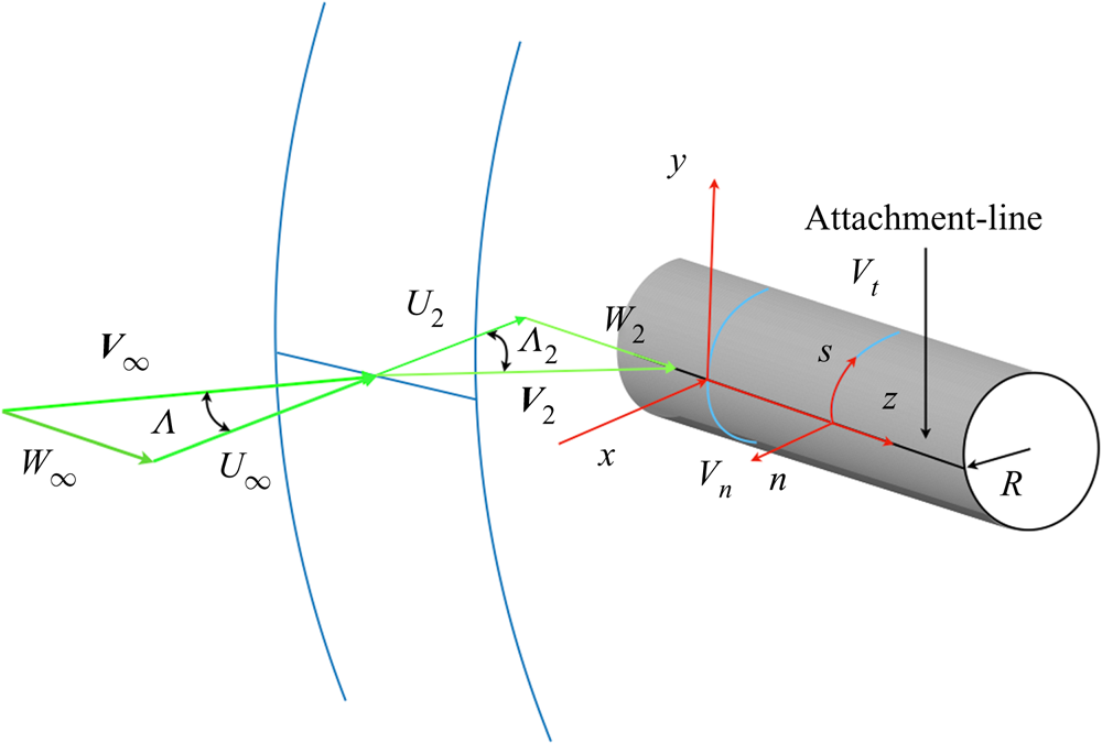
Figure 1. Schematic of hypersonic flow around an inclined cylinder. The velocity vector ahead of the shock is  ${\boldsymbol {V}}_{\infty }=(U_{\infty },V_{\infty },W_{\infty })$ and
  ${\boldsymbol {V}}_2 = (U_{2},V_{2},W_{2})$ is the velocity vector behind the shock,
  $V_t$ and
  $V_n$ represent the velocity along the surface tangential direction
  $s$ and wall-normal direction
  $n$, and
  $\varLambda$ and
  $\varLambda _2$ represent the sweep angles in the free stream and behind the shock.
Following the previous studies by Mack et al. (Reference Mack, Schmid and Sesterhenn2008) and Mack & Schmid (Reference Mack and Schmid2011a), we define a free-stream Reynolds number  $Re_{\infty }$, a sweep Reynolds number
  $Re_s$, a free-stream Mach number
  $M_{\infty }$, a sweep Mach number
  $M_s$ and a recovery temperature
  $T_r$ as,
 \begin{equation} \left.\begin{gathered} Re_{\infty} = \frac{|{\boldsymbol{V}}_{\infty}| \delta}{\nu_{\infty}},\quad Re_s = \frac{W_2 \delta}{\nu_r},\quad M_{\infty} = \frac{|{\boldsymbol{V}}_{\infty}| }{c_{\infty}},\quad M_s = \frac{W_2}{c_2}, \\ T_r = T_{\infty} + \sigma (T_0 - T_{\infty}),\quad \textrm{where}\ \sigma = 1 - (1 - \xi_w) \sin^2\varLambda. \end{gathered}\right\} \end{equation}
In (2.1),  $\xi _w$ is a constant for specific free-stream conditions (
 $M_{\infty }$ and
  $\varLambda$) and determined based on the study of Reshotko & Beckwith (Reference Reshotko and Beckwith1958). The parameter
  $c$ is the speed of sound,
  $\nu _r$ represents the kinematic viscosity at the recovery temperature
  $T_r$. The viscosity lengths scale
  $\delta$ is determined as
 \begin{equation} \delta =\sqrt{\frac{\nu_r R}{2U_2}}. \end{equation}
The free-stream Mach number  $M_\infty =7.14$ and temperature
  $T_{\infty } = 69.84\ \textrm {K}$ are fixed for all cases. A cold wall temperature is specified as
  $T_w = 0.4 T_r$ according to experimental conditions. The Prandtl number
  $Pr=0.72$ and the specific heat ratio
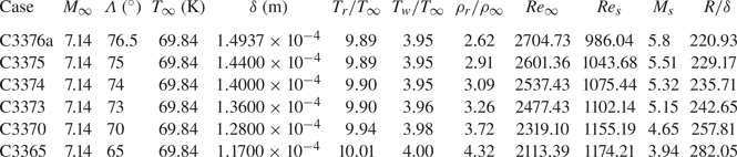
  $\gamma =1.4$ is defined following the ideal gas assumption of air. The defined six cases are listed in table 1. These cases differ in sweep angles, leading to different length scales
  $\delta$ and different sweep Mach numbers
  $M_s$. Other parameters are listed in table 1. As most high-order finite difference methods (Lele Reference Lele1992; Zhong Reference Zhong1998; Mack & Schmid Reference Mack and Schmid2010a) for solving NS/Euler equations need to reduce the scheme order at boundary regions to satisfy the dissipation-error and stability conditions, the full-size model is used to maintain the scheme order around the attachment line, even though the flow is symmetric to the
  $x$–
$x$– $z$ plane at
  $y=0$ at zero angle of attack. Note that there are generally two choices when solving the laminar basic flow. The most appropriate is the DNS which solves the NS equation with high-order shock fitting methods (Moretti Reference Moretti1987; Zhong Reference Zhong1998; Kopriva Reference Kopriva1999), therefore, taking all the information into account. The other is the combination of solving inviscid Euler equation and boundary layer equations (see Theofilis et al. Reference Theofilis, Fedorov and Collis2006 and Wang et al. Reference Wang, Wang, Wang, Xu and Fu2018 for more details), which is much cheaper but overlooks the influence of the inviscid flow outside the boundary layer. Both methods (DNS and boundary layer assumption) are used and compared in the present study.
Table 1. Parameters of the flow cases in the current study. The names of cases are the same as in the experiment of Gaillard et al. (Reference Gaillard, Benard and Alziary de Roquefort1999). The ‘C’ represents the cylinder. The first two number represent the radius and the last two numbers stand for the sweep angle. Here  $\rho _r$ is the density of the fluid at the recovery temperature
  $T_r$ and
  $\rho _{\infty }$ represents the density of the free stream.
2.2. Mathematical formulation
2.2.1. Flow governing equations
The problem solution starts from the unsteady three-dimensional NS equations:
 \begin{gather} \frac{\partial Q}{\partial t}+\frac{\partial F_j}{\partial x_j} + \frac{\partial F_{vj}}{\partial x_j}=0, \end{gather}
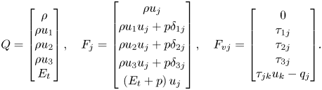 \begin{gather}Q = \begin{bmatrix} \rho \\ {\rho {u_1}} \\ {\rho {u_2}} \\ {\rho {u_3}} \\ {{E_t}}\end{bmatrix},\quad {F_j} = \begin{bmatrix} {\rho {u_j}} \\ {\rho {u_1}{u_j} + p{\delta _{1j}}} \\ {\rho {u_2}{u_j} + p{\delta _{2j}}} \\ {\rho {u_3}{u_j} + p{\delta _{3j}}} \\ {\left( {{E_t} + p} \right){u_j}}\end{bmatrix},\quad{F_{vj}} = {\begin{bmatrix} 0 \\ {{\tau _{1j}}} \\ {{\tau _{2j}}} \\ {{\tau _{3j}}} \\ {{\tau _{jk}}{u_k} - {q_j}} \end{bmatrix}}. \end{gather}
The total energy  $E_t$ and the viscous stress
  $\tau _{ij}$ are given as, respectively,
 \begin{equation} E_{t}=\rho\left(\frac{T}{\gamma(\gamma-1) M^{2}_{\infty}}+\frac{u_{k} u_{k}}{2}\right), \quad \tau_{i j}=\frac{\mu}{Re_{\infty}}\left(\frac{\partial u_{i}}{\partial x_{j}}+\frac{\partial u_{j}}{\partial x_{i}}-\frac{2}{3} \delta_{i j} \frac{\partial u_{k}}{\partial x_{k}}\right). \end{equation}
The pressure  $p$ and heat flux
  $q_i$ are obtained from
 \begin{equation} p=\frac{\rho T}{\gamma M_{\infty}^{2}}, \quad q_{i}={-}\frac{\mu}{(\gamma-1) M_{\infty}^{2} Re Pr} \frac{\partial T}{\partial x_{i}}. \end{equation}
The viscosity is calculated using the Sutherland law
 \begin{equation} \mu = T^{3/2}\frac{T_{\infty} + C}{T T_{\infty} + C}, \end{equation}
with  $C = 110.4\ \textrm {K}$. The fifth-order upwind scheme (for inviscid flux
  $F_{j}$) of Zhong (Reference Zhong1998) together with the sixth-order centre scheme (for viscous flux
  $F_{vj}$) is used to compute the flow field. Here, the non-conservative characteristic relation is adapted at the shock surface for more convenient stability analysis, because we perform the stability analysis based on primitive variables. A fourth-order Runge–Kutta method is applied for the time integration. By treating the shock wave as a sharp interface, high accuracy can be achieved in the whole flow field, which is an essential prerequisite for the stability analysis. The Euler equation is solved by the same method by ignoring the viscous flux
  $F_{vj}$.
Once the basic flow is obtained, the linear Navier–Stokes (LNS) equation of the perturbations are solved. The LNS equations are derived from the NS equations by introducing small perturbations, subtracting the basic flow equations and ignoring the nonlinear terms. A frequently employed form is commonly written as
 \begin{align} &{\boldsymbol{\varGamma}}\frac{\partial \boldsymbol{\varPhi}}{\partial t} +\boldsymbol{A} \frac{\partial \boldsymbol{\varPhi}}{\partial x}+\boldsymbol{B}\frac{\partial \boldsymbol{\varPhi}}{\partial y} +\boldsymbol{C}\frac{\partial \boldsymbol{\varPhi}}{\partial z}+ \boldsymbol{D}\boldsymbol{\varPhi}\nonumber\\ &\quad = \boldsymbol{H}_{xx}\frac{\partial^2 \boldsymbol{\varPhi}}{\partial x^2}+\boldsymbol{H}_{xy}\frac{\partial^2 \boldsymbol{\varPhi}}{\partial x\partial y} +\boldsymbol{H}_{xz}\frac{\partial^2 \boldsymbol{\varPhi}}{\partial x\partial z}+\boldsymbol{H}_{yy}\frac{\partial^2 \boldsymbol{\varPhi}}{\partial y^2} +\boldsymbol{H}_{yz}\frac{\partial^2 \boldsymbol{\varPhi}}{\partial y\partial z}+\boldsymbol{H}_{zz}\frac{\partial^2 \boldsymbol{\varPhi}}{\partial z^2}, \end{align}
where the coefficient matrix  ${\boldsymbol {\varGamma }},{\boldsymbol {A}},{\boldsymbol {B}}, {\boldsymbol {C}},{\boldsymbol {D}},{\boldsymbol {H}}_{xx}, {\boldsymbol {H}}_{xy},{\boldsymbol {H}}_{xz},{\boldsymbol {H}}_{yy}, {\boldsymbol {H}}_{yz},{\boldsymbol {H}}_{zz}$ can be found in (Ren & Fu Reference Ren and Fu2014, Reference Ren and Fu2015; Wang, Wang & Fu Reference Wang, Wang and Fu2017).
2.2.2. Linear local stability approach
For local analysis, the perturbations along the attachment-line can be written in a wave-like form as
 \begin{equation} \boldsymbol{\varPhi}(x,y,z,t) = \boldsymbol{\phi}(x)\exp\left(\textrm{i}\alpha y + \textrm{i}\beta z - \textrm{i}\omega t\right) + \textrm{c.c.}, \end{equation}
where  $\boldsymbol {\phi } = (\rho ',u',v',w',T')$ is the shape function,
  $\alpha$ and
  $\beta$ are the wave numbers along
  $y$ and
  $z$ directions,
  $\omega$ is the frequency and c.c. represents the complex conjugate. As
  $\alpha$ is not known a priori for local calculations, a two-dimensional perturbation wave assumption is used here as
  $\alpha = 0$. Substituting (2.9) into (2.8), the LNS reduces to a generalized eigenvalue problem as
 \begin{equation} \mathfrak{L}_l\boldsymbol{\phi} = \omega\mathfrak{R}_l\boldsymbol{\phi}, \end{equation}
where  $\mathfrak {L}_l$ and
  $\mathfrak {R}_l$ are matrix operators:
 \begin{gather} \mathfrak{L}_l=(\boldsymbol{D} + \textrm{i}\beta \boldsymbol{C} + \beta^2\boldsymbol{H}_{zz}) +\left(\boldsymbol{A}-\textrm{i}\beta \boldsymbol{H}_{xz}\right)\frac{\partial}{\partial x} - \boldsymbol{H}_{xx}\frac{\partial^2}{\partial x^2}, \end{gather}
 \begin{gather}\mathfrak{R}_l =\textrm{i}{\boldsymbol{\varGamma}}. \end{gather}
A temporal stability analysis is performed considering the homogeneous nature in the spanwise direction. In the wall-normal direction, grids cluster near the wall surface in the following manner
 \begin{equation} y=a\frac{1+\eta}{b-\eta},\quad\text{with}\ a=\frac{y_iy_{max}}{y_{max}-2y_{i}},\quad b=1+\frac{2a}{y_{max}},\quad \eta\in\left[{-}1,1\right], \end{equation}
where  $y_{max}$ represents the far-field and
  $y_i$ is the control point. This grid distribution allows for clustering of half of the grid points in the region
  $\left [0,y_i\right ]$, as first used by Malik (Reference Malik1990). The spectral method is used for approximation of the derivatives and a standard QZ solver (Golub & Van Loan Reference Golub and Van Loan2013) is used for solving the eigenvalue problems.
2.2.3. Global stability approach
From the global point of view, perturbations can be written in a more general form:
 \begin{equation} \boldsymbol{\varPhi}(x,y,z,t) = \boldsymbol{\phi}(x,y)\exp\left(\textrm{i}\beta z - \textrm{i}\omega t\right) + \textrm{c.c.} \end{equation}
Substituting (2.14) into (2.8), one again arrives at a generalized eigenvalue problem,
 \begin{equation} \mathfrak{L}\boldsymbol{\phi} = \omega\mathfrak{R}\boldsymbol{\phi}, \end{equation}
where  $\mathfrak {L}$ and
  $\mathfrak {R}$ are matrix operators:
 \begin{gather} \mathfrak{L}=\left(\boldsymbol{D}+\textrm{i}\beta \boldsymbol{C} + \beta^2\boldsymbol{H}_{zz}\right)+ \left(\boldsymbol{A}-\textrm{i}\beta \boldsymbol{H}_{xz}\right)\frac{\partial}{\partial x}+ \left(\boldsymbol{B}-\textrm{i}\beta \boldsymbol{H}_{yz}\right)\frac{\partial}{\partial y} \nonumber\\ \hspace{-7pc} -\boldsymbol{H}_{yy}\frac{\partial^2}{\partial y^2}-\boldsymbol{H}_{xy} \frac{\partial^2}{\partial x\partial y} - \boldsymbol{H}_{xx}\frac{\partial^2}{\partial x^2}, \end{gather}
 \begin{gather} \mathfrak{R}=\textrm{i}{\boldsymbol{\varGamma}}. \end{gather}
Considering the length scale of instability of the previous study (Mack et al. Reference Mack, Schmid and Sesterhenn2008; Mack & Schmid Reference Mack and Schmid2010a, Reference Mack and Schmid2011a,Reference Mack and Schmidb), the basic non-dimensional spanwise wave number  $\beta$ is chosen to be
  $0.3$. Because the matrices discretizing the global stability problem have leading dimensions of
  $O(10^5\text {--}10^6)$, instead of classical QZ method, a Krylov–Shur method (Stewart Reference Stewart2002a,Reference Stewartb), based on PETSc (http://www.mcs.anl.gov/petsc) and SLEPc (http://slepc.upv.es) with various spectral transformation techniques have been used to recover a window (100–400) of the eigenvalues of interest. The Krylov–Shur method, which is another kind of implicitly restarted Arnoldi algorithm, can achieve very high precision for specific part of the spectrum with proper spectral transformations. Sparse linear algebra packages, MUMPS (http://mumps.enseeiht.fr) and SuperLU (https://portal.nersc.gov/project/sparse/superlu/) are used to undertake the inverse of a matrix during the spectral transformations. In both directions, special mesh distribution (FD-q grids) based on Hermanns & Hernandez (Reference Hermanns and Hernandez2008) is implemented according to the order of the scheme as first discussed by Paredes et al. (Reference Paredes, Hermanns, Le Clainche and Theofilis2013). Again, FD-q grids cluster near the wall surface using (2.12) and an eighth-order FD-q scheme is used.
2.2.4. Boundary conditions
In the basic flow, a no-slip boundary condition together with the isothermal wall on the cylinder surface are employed. At the end of chordwise or surface tangential direction for the computational domain, characteristic non-reflect boundary conditions are imposed. In the calculation of perturbations, no-slip and Dirichlet conditions for temperature are specified at the wall ( $(u',v',w',T')= 0$). At the far field (on the shock surface) all perturbations except density are forced to zeros. Along the
  $s$ direction, at the exit, a high-order extrapolation is performed from interior for all perturbation quantities.
3. Basic flow
The present analysis covers sweep Mach number  $M_s$ roughly from 4 to 6 as listed in table 1. Owing to the discrepancy in shock shapes, computation domains are therefore different among cases. For all cases, a mesh is generated with: 641 grid points in the surface direction (clustered around the leading edge), 221 grid points in the wall-normal direction (at least 35 points clustered inside the boundary layer) and 8 grid points in the spanwise direction due to the homogeneous nature in this flow. Compared with previous DNS study (Speer et al. Reference Speer, Zhong, Gong and Quinn2004; Mack et al. Reference Mack, Schmid and Sesterhenn2008), the basic flow can be adequately resolved under this grid resolution.
The evolution of the maximum density residual as a function of the number of time steps is shown in figure 2. The small initial residual level is due to the well-converged initial field from the preliminary calculation using first-order upwind scheme. After several millions of steps, when the residual reaches the machine accuracy, this ‘steady state’ is considered as converged. From figure 2, one can find that cases with higher Reynolds number  $Re_{\infty }$ converge slower. More time steps are consequently needed by the flow to adjust to the much thicker boundary layers where viscous effects are stronger.
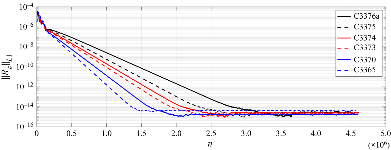
Figure 2. Converging history of the basic flow calculations with high-order shock-fitting method. The vertical axis represents the maximum residual  $||R_{\rho }||_{L_1}$ in density
  $\rho$.
The flow field of C3365 case is visualized in figure 3 to illustrate key features of the flow cases. As can be observed, the curved streamlines in the  $x$–
$x$– $y$ cross-plane around the cylinder together with the large spanwise velocity, represent a typical three-dimensional flow, especially at the leading edge. The density distributions of the basic flow for all cases are shown in figure 4. At the leading edge, as the sweep angle becomes large, the shock is moving away from the wall surface and the shock standoff distance, the distance between the shock surface and attachment line, increases from around
  $0.7R$ to
  $2.2R$. The profiles of the main physical components of the attachment-line boundary layer are shown in figure 5. Two major features should be noticed. First, as sweep Mach numbers increase, the thickness of the boundary layer increases. Second, interestingly, in the profiles of the
  $U$-velocity component, a distinct contortion is observed near the outer edge of the boundary layer. Also there, the temperature
  $T$ and density
  $\rho$ profiles exhibit variations that were not found in the solution of the boundary layer equations (see Appendix C). The basic flow obtained with traditional boundary layer assumptions is given in Appendix C. It will be seen there that the differences in the basic flows are significant giving rise to the findings of the attachment-line modes. The profile of
  ${\partial }/{\partial h}(\rho ({\partial W}/{\partial h}))$ at attachment line from C3376a case is shown in figure 6. By comparing profiles from the boundary layer approximations and the full NS solution, the major differences between these two solutions can be easily found and two generalized inflection points, where
  ${\partial }/{\partial h}(\rho ({\partial W}/{\partial h}))=0$, are seen in figure 6 in the NS solution.
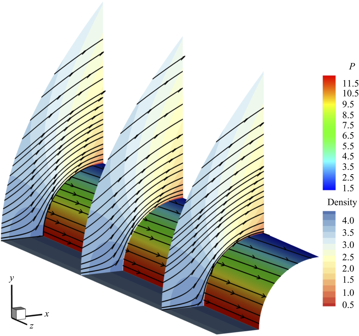
Figure 3. Contours of basic flow density at three spanwise locations together with pressure contour over cylinder wall surface. Streamlines are also plotted on these contours.
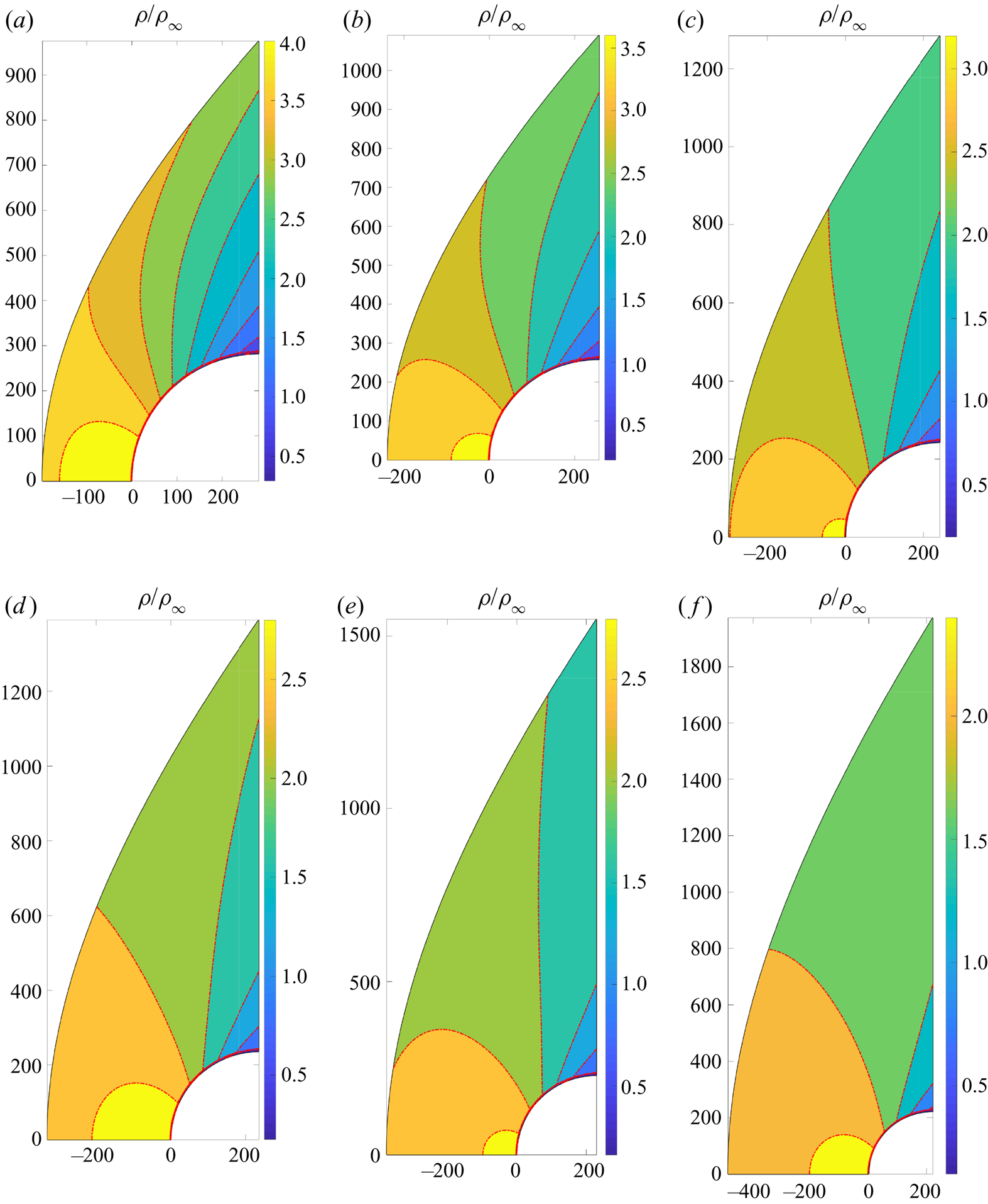
Figure 4. Density contours over  $x$–
$x$– $y$ plane for all cases: (a–f) represent the cases from C3365 with sweep Mach number
  $M_s= 3.94$ to C3376a of
  $M_s=5.8$. Only the upper half plane is shown because of symmetry.
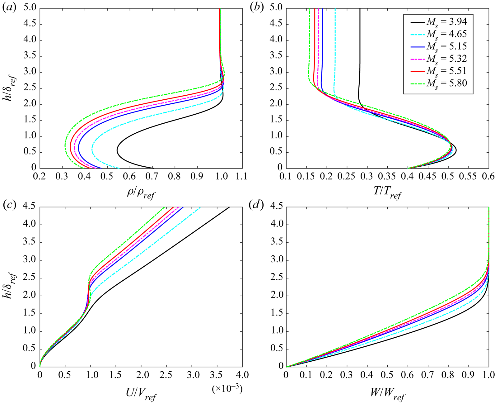
Figure 5. Variation of the basic flow profiles with different sweep Mach numbers: (a–d) represent the  $\rho ,T$,
  $U$ and
  $W$ profiles, respectively. All reference values are defined at the edge of stagnation boundary layer except for temperature. The reference temperature takes the recovery temperature. Here
  $\delta _{ref} = \delta$ and
  $h$ represents the distance away from the attachment line.
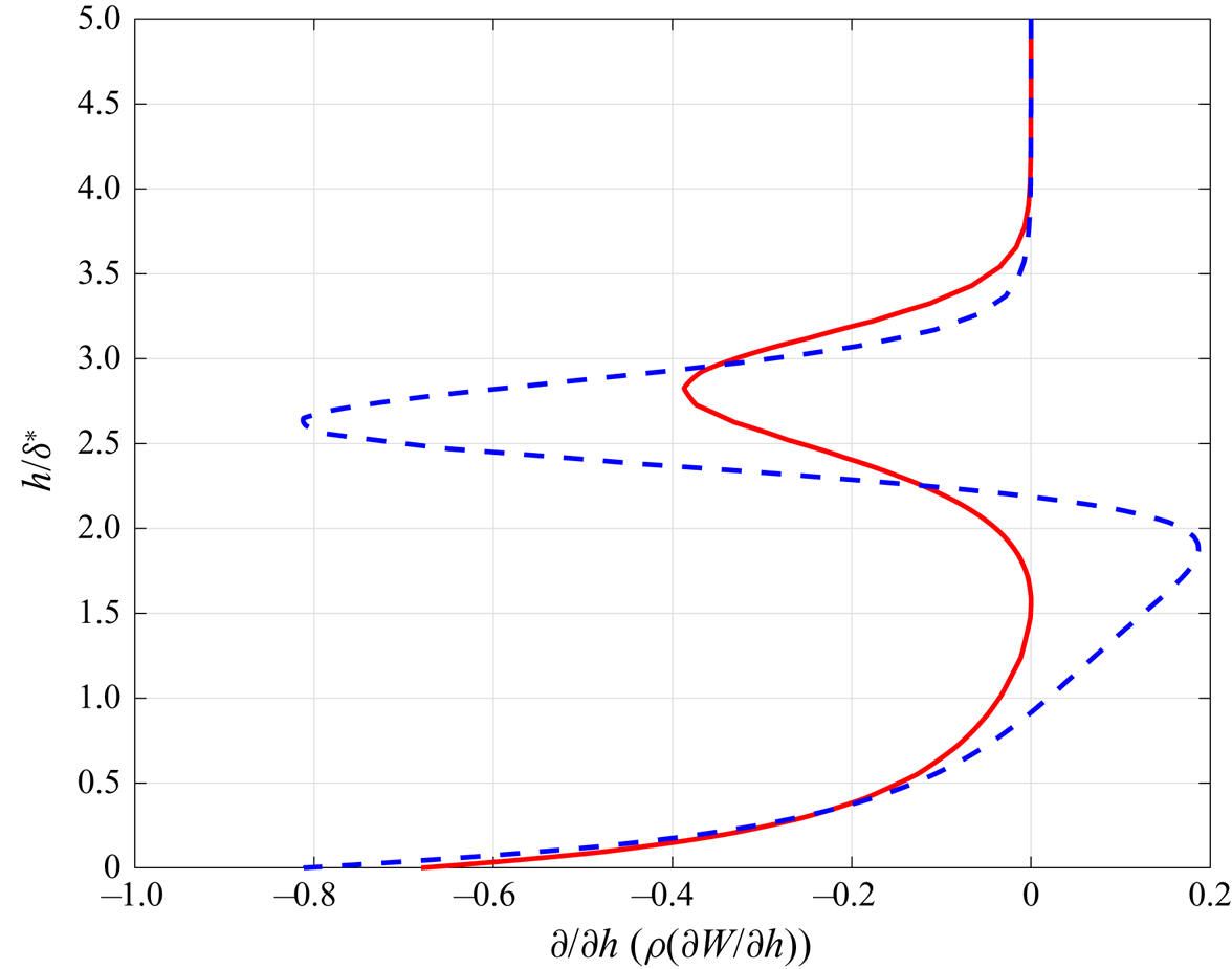
Figure 6. The profiles of  ${\partial }/{\partial h}( \rho ({\partial W}/{\partial h}))$ along wall-normal distance
  $h/\delta ^*$ from the attachment line for C3376a case with
  $M_s=5.8$. The solid red line represents the result from the boundary layer approximation and the dashed blue line the result from the full NS equation.
Along the surface far from the attachment line, velocity profiles and pressure gradient at five different locations are shown in figure 7. An inflection point appears along with the presence of tangential velocity overshoot in figure 7(a), which is a typical phenomenon of a boundary layer subject to pressure gradient and surface heat transfer (Cohen & Reshotko Reference Cohen and Reshotko1956). Along the surface, together with the development of the boundary layer, the spanwise profile becomes thicker (figure 7c), and the wall-normal velocity profile turns from negative to positive (figure 7b). The surface pressure gradient is also shown in figure 7(d) and over the whole surface the fluid is accelerated continuously.
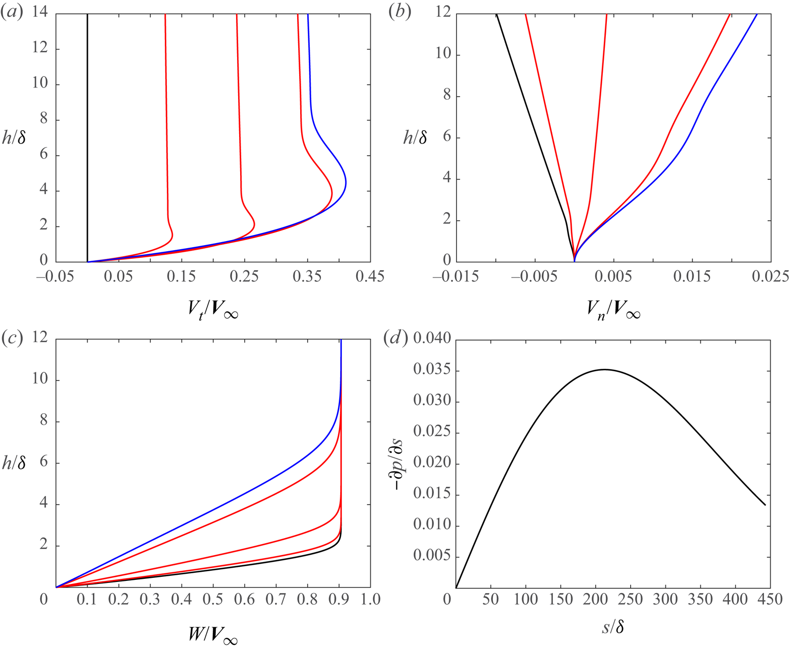
Figure 7. Profiles of velocity components and pressure gradient in the surface direction for case C3365: (a–c) show the tangential velocity  $V_t$, the normal velocity
  $V_n$ and the sweep velocity
  $W$ profiles along the surface from the attachment line (black lines,
  $s=0$) to the exit (blue lines,
  $s= 443.04$), respectively. Red lines, between the black and the blue, represent the velocity profiles at three increasing locations
  $s = 138.93$, 277.86 and 416.79, respectively. The pressure gradient along the surface is shown in (d). Here
  $h$ represents the distance away from surface.
4. Stability analysis
In the present stability analysis, the behaviours of the perturbations at the attachment line are obtained both locally and globally. First, the local analysis is performed along the attachment line based on the profiles from the previous full NS calculation. Two sets of grids (401 and 801 points in the wall-normal direction,  $n$), together with the spectral methods, had been employed to achieve the mesh-independent solution and to reveal the structure of the spectrum. Figure 8 shows the typical eigenspectrum of case C3376a, for illustration, based on the profiles from DNS calculation and the solution based on boundary layer approximation is also shown for comparison. Other cases have similar features. Two discrete modes are identified and marked in this figure and no unstable discrete mode is found when the basic flow is calculated with boundary layer equations. The unstable discrete mode is located around the continuous branch of the slow acoustic wave (the left red line). The stable discrete mode is found at around the fast acoustic wave (the right red line). The distribution of the spectrum is similar to that obtained from the boundary layer approximation (green points in figure 8). Based on the previous study of hypersonic flat boundary layers over a cold wall (Fedorov & Tumin Reference Fedorov and Tumin2003, Reference Fedorov and Tumin2011), the spectra of perturbations are made of continuous spectra, which are smooth branch cuts over the complex plane, and of discrete spectra which are poles locating around these branches. However, in the present cases, because of the variations of basic flow outside the boundary layer, the shape of the continuous spectrum changes significantly when more grids are used.
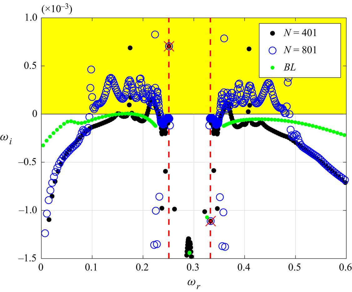
Figure 8. Spectral distribution based on local analysis for C3376a case ( $M_s=5.8$). The unstable region is marked in yellow. Two different grids had been used to cross-validate the results, and the discrete eigenvalues are marked by red crosses. Two red dashed lines represent the locations of slow acoustic branch (left) and fast acoustic branch (right). The spectrum from the boundary layer solution is shown by green points.
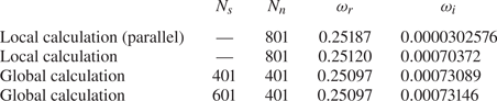
The eigenfunctions of this case are shown in figure 9 and the relative eigenvalue of unstable mode is listed in table 2. Comparing the eigenvalues with local parallel approximation, we can find that the small velocity component  $U$, in the
  $x$–
$x$– $y$ plane is vital for this instability, as the growth rate predicted by parallel approximation theory is one order smaller than others. All perturbations are normalized with their maximum norm. The perturbations are mainly distributed inside the boundary layer and become significant near the boundary layer edge. The perturbations of temperature and density have their peak near the location
  $h/\delta = 2.1$. Outside of the boundary layer, perturbations decay as usual. For unstable modes, indicated as blue dashed lines and black lines, the results from the local calculation and the global calculation agree well. The shape of the unstable eigenfunctions from the global calculation are similar to those from the local calculation inside the boundary layer, but decay much faster outside of the boundary layer, which can be seen in figure 9(b). Following the study of Mack (Reference Mack1984), we further define the locations of the critical layer (
 $c_r^{a} = \bar {U}$) and the sonic line (
 $c_r^{a} = \bar {U} + a$) at the attachment line, where
 \begin{equation} c_r^{a} = \frac{\omega}{\beta},\quad \bar{U} = W,\quad a = \frac{\sqrt{T}}{M_{\infty}}. \end{equation}
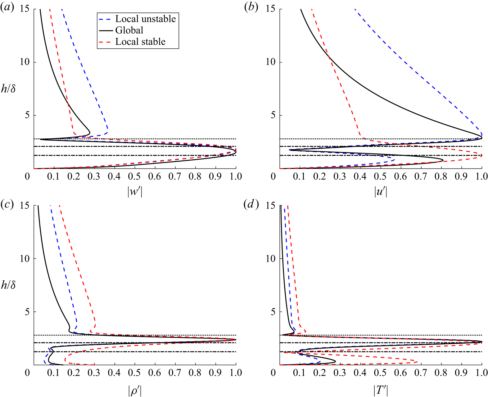
Figure 9. Comparisons of normalized perturbation profiles from the attachment line with the solid black line from global stability analysis and dashed blue/red lines from local stability analysis for the C3376a case ( $M_s=5.8$). The dashed blue and red lines represent the eigenfunctions of unstable and stable discrete modes, respectively. All the eigenfunctions are normalized by the maximum norm with (a) spanwise velocity perturbation
  $|w'|$, (b) wall-normal velocity perturbation
  $|u'|$ and (c,d) density and temperature perturbations. The horizontal black dotted lines, located around
  $h/\delta = 2.80$, represent the edge of the boundary layer. The two horizontal black dash-dotted lines represent the location of critical layer (located around
  $h/\delta =2.1$, top) and sonic line (located around
  $h/\delta =1.25$, bottom).
Table 2. Comparison of the local stability with the global results for the case C3376a ( $M_s=5.8$). Here
  $N_s$ and
  $N_n$ represent the grid points along the surface and wall-normal direction, respectively.
The existence of a relative supersonic region (below the sonic lines) shown in figure 9 and the generalized inflection points of basic flow shown in figure 6 indicate that the present mode can be seen as a combination of inviscid instability owing to a generalized inflection point and supersonic relative basic flow.
In reality, physical perturbations consist of waves with various wave numbers. It is thus meaningful to investigate the reliance of local growth rates to spanwise wave numbers. To also compare results among different cases, a dimensional spanwise wave number  $\beta ^* = \beta / \delta$ is used. As shown in figure 10, when the sweep Mach number increases from 3.94 in C3365 to 5.8 in C3376a, the unstable region is broadened and the local growth becomes larger. This finding is totally different from low-speed situation. For subsonic flow, as reported by Gennaro et al. (Reference Gennaro, Rodríguez, Medeiros and Theofilis2013), when the sweep Mach number decreases the growth rate increases. Moreover, for the cases with low spanwise Mach numbers, 3.94 in C3365 and 4.65 in C3370, the leading discrete modes are absorbed into continuous branches at small
  $\beta ^*$ and cannot be tracked as shown by the blue lines in figure 10.
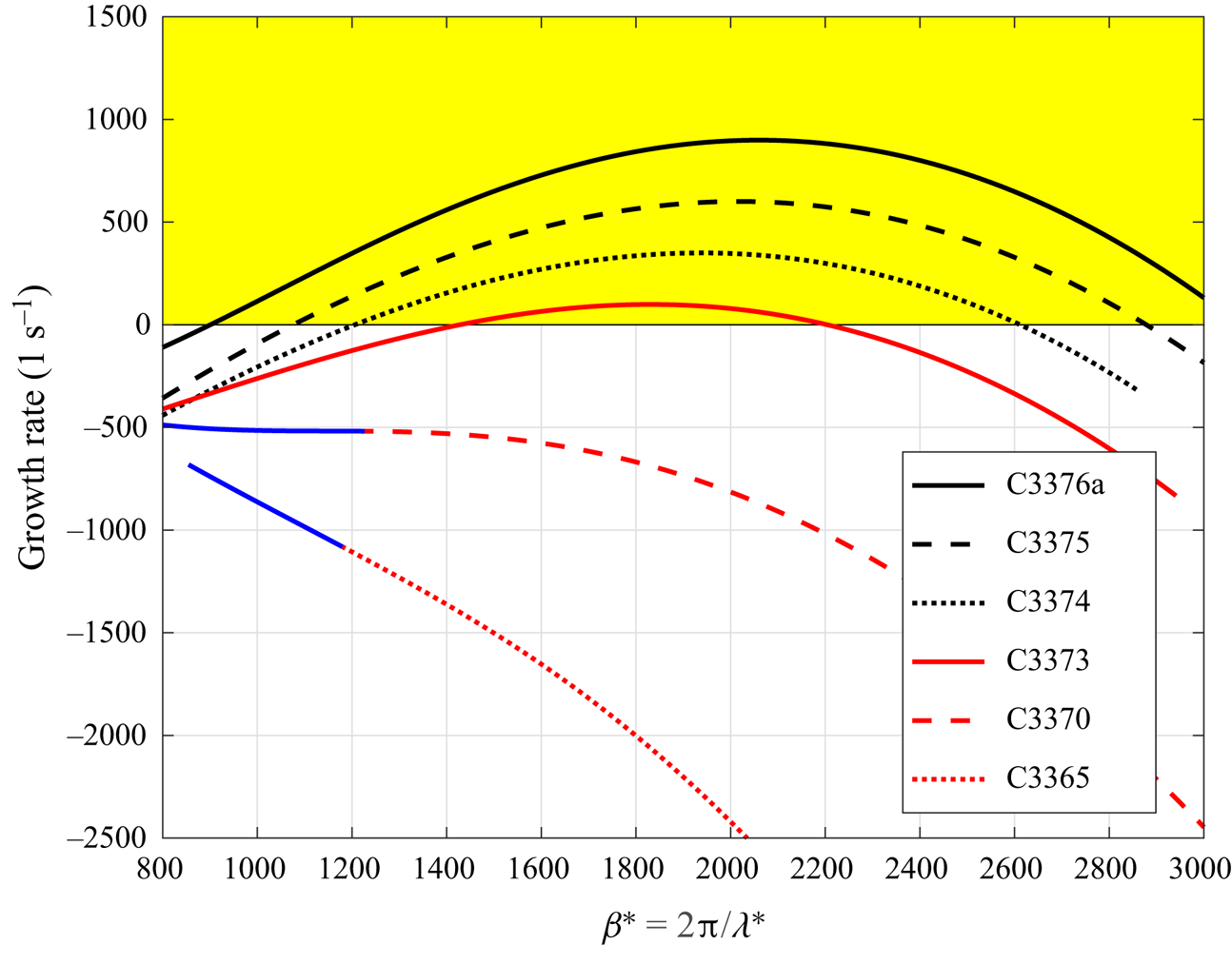
Figure 10. Variations of growth rate of leading boundary modes with spanwise wave numbers for all cases. The blue lines represent regions where the discrete modes are absorbed into continuous branches. Here  $\lambda ^*$ represent the dimensional wavelength of the perturbations along
  $z$ direction.
Further comparison of the maximum growth rates of various sweep Mach numbers with the transition detections from experiments is shown in figure 11. As reported in the experiment (Gaillard et al. Reference Gaillard, Benard and Alziary de Roquefort1999), when the sweep Mach number increases from around 3.5 to 6, the transition Reynolds number defined by Poll (Reference Poll1979) decreases continuously. The theoretical growth rate increases continuously under similar conditions. Because the flow is homogeneous in spanwise direction  $z$, the unstable perturbation will eventually degenerate into transition. Considering the differences between experiments and theoretical predictions, the tendency of the flow instability to the sweep Mach number is the same for both experimental and theoretical works. This explains why the critical transition Reynolds number decreases when the sweep Mach number is above 5. Together with the analysis of basic flow (see figure 6), this attachment-line mode is different from incompressible cases (Theofilis Reference Theofilis1995, Reference Theofilis1998; Lin & Malik Reference Lin and Malik1996, Reference Lin and Malik1997; Obrist & Schmid Reference Obrist and Schmid2003a,Reference Obrist and Schmidb; Theofilis et al. Reference Theofilis, Fedorov, Obrist and Dallmann2003). Traditional attachment-line modes for low-speed compressible flow can be treated as a kind of three-dimensional TS waves that belong to viscous instability (Lin & Malik Reference Lin and Malik1995). Based on the velocity profiles at attachment line (figure 5), the major basic flow components along the line are the density, temperature and spanwise velocity. The velocity components in the
  $x$–
$x$– $y$ plane are a few orders of magnitude smaller than the spanwise velocity and can be ignored from the leading term analysis (see Appendix D). Thus, the boundary layer along the attachment line can be seen as a parallel flow and is similar to the boundary layer along a flat plate. As a result of the classical inviscid theory (Lees & Lin Reference Lees and Lin1946; Mack Reference Mack1984), the attachment-line mode found in this study belongs to the inviscid instability.
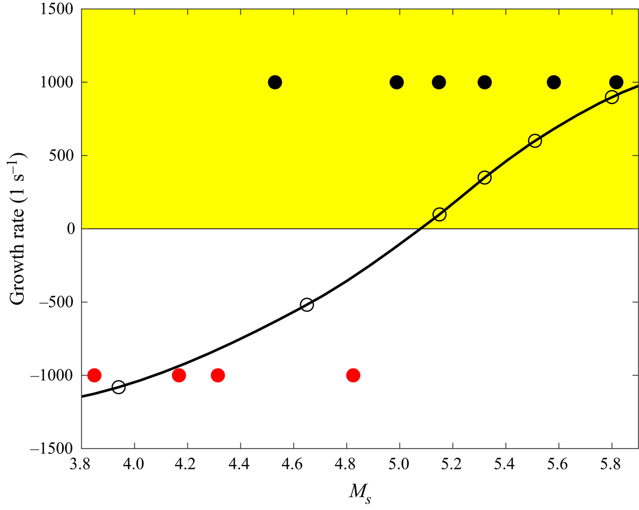
Figure 11. Variation of the leading boundary modes with sweep Mach number. The solid black dots represent the cases where transition was detected at the attachment line in the experiments (Gaillard et al. Reference Gaillard, Benard and Alziary de Roquefort1999) whereas the solid red dots indicate no transition. The black line with the circles is the result from the local analysis.
The major limitation in local stability theory is the neglection of the multi-dimensional effect which can be easily identified in the basic flow (figure 3). In particular, in the vicinity of the attachment line, flow impingement rather than shear is the dominant feature. In contrast, non-negligible variations of basic flow with respect to the  $y$ direction, the curvature effects around the attachment line and the features of further downstream region can all be taken into account properly by the global stability analysis.
The global instabilities are performed on a very fine FD-q grids with 601 grid points along the surface tangential direction  $s$ and
  $401$ grid points on the wall-normal direction
  $n$ over the
  $x$–
$x$– $y$ cross-section plane. Compared with the results from coarser grids (as listed in table 2), this resolution (
 $601\times 401$) can well capture the main feature of the global instabilities. The calculated eigenspectrum are shown in figure 12 for the four most dangerous cases at sweep Mach number greater than 5.
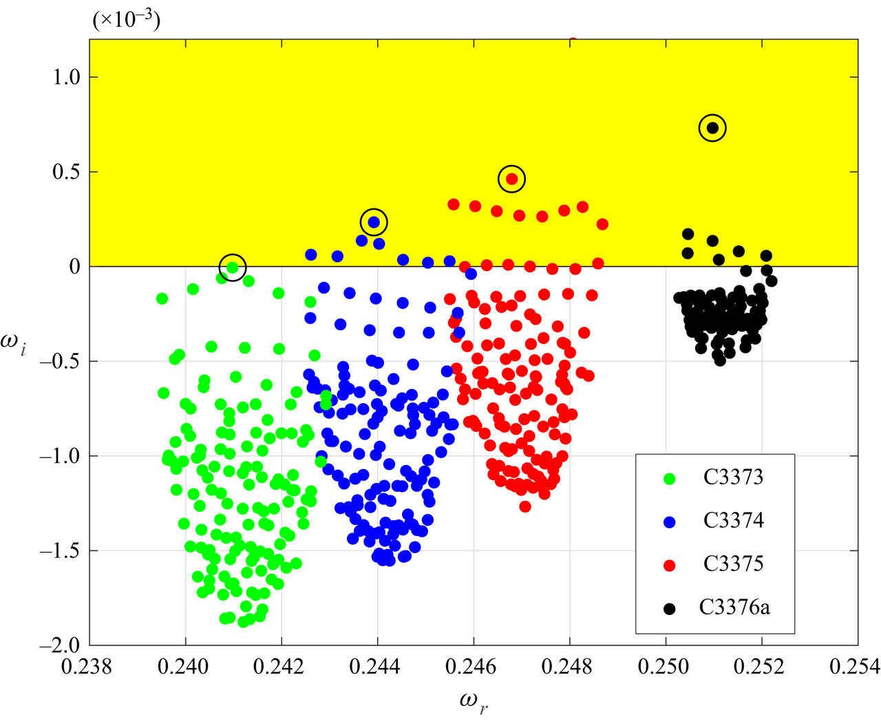
Figure 12. The calculated spectra around the leading attachment-line modes for sweep Mach numbers 5.8 (C3376a), 5.51 (C3375), 5.32 (C3374) and 5.15 (C3373). The leading eigenvalues are marked by black circles.
The dependence of  $\omega _i$ on the spanwise wave number
  $\beta$ is shown in figure 13 for both local and global calculations. It is seen here that the results from these two analyses agree reasonably well at wave number roughly greater than 0.2085. Below this value, the global growth rate drops much faster than local calculations. In fact, the global calculation indicates that the mode is unstable in the region
  $0.178 <\beta < 0.461$. The maximum global growth rate is slightly larger than the local analysis. The major difference of local and global analysis for this case is the leading-edge effect of the stability equation, flow impingement and curvature effects of the basic flow are included in the solution of NS equations. Thus, for small spanwise wave number
  $\beta$ the leading-edge curvature has a stabilizing effect but a destabilizing effect when the wave number is larger in the unstable region. This finding is different from the results for incompressible flows, where the leading-edge curvature exhibits a stabilizing effect on the attachment-line boundary layer (Lin & Malik Reference Lin and Malik1997).
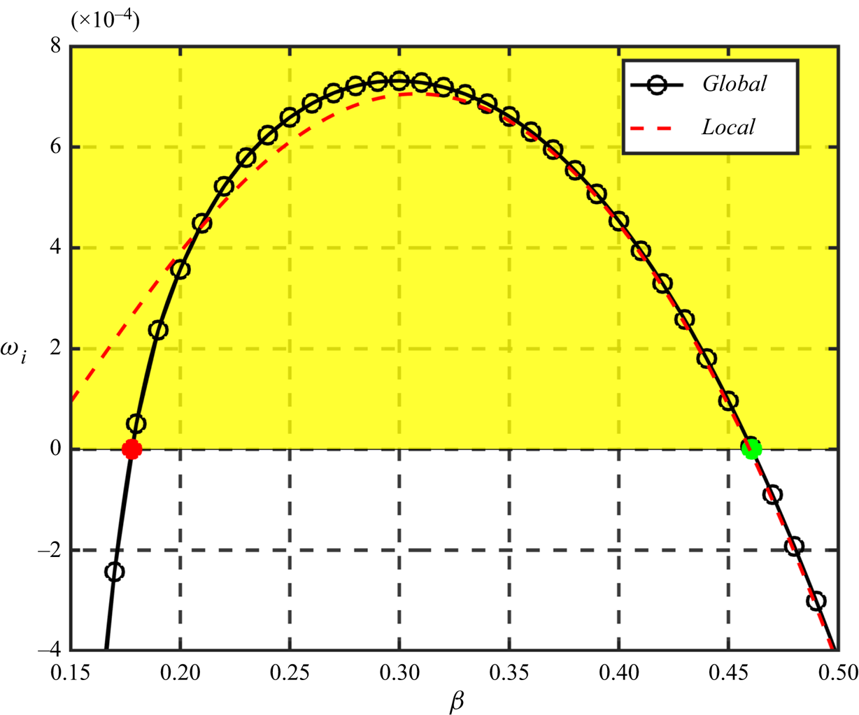
Figure 13. Dependences of  $\omega _i$ on the spanwise wave number
  $\beta$ for C3376a case with
  $M_s=5.8$. The black line with black circles represents the results from global calculations and the red dashed line represents the results from local calculation. The red and green dots represent two critical values.
In global analysis, the temporal behaviour is reflected in the eigenvalues  $\omega = \omega _r + i\omega _i$ whose imaginary part shows whether the perturbation grows or decays with time. The spatial behaviour is represented by the eigenfunctions. Perturbation profiles at different
  $s$-surface locations are shown in figure 14. Among all the perturbations, the temperature and density have the maximum amplitudes. The velocity perturbations, though having much smaller amplitudes, are critical for the transport of low- and high-momentum fluid. Together with the development of the boundary layer, perturbations move away from the wall. From the attachment-line region to further downstream location, both the amplitude and the affected area of velocity perturbations grow (figure 14).
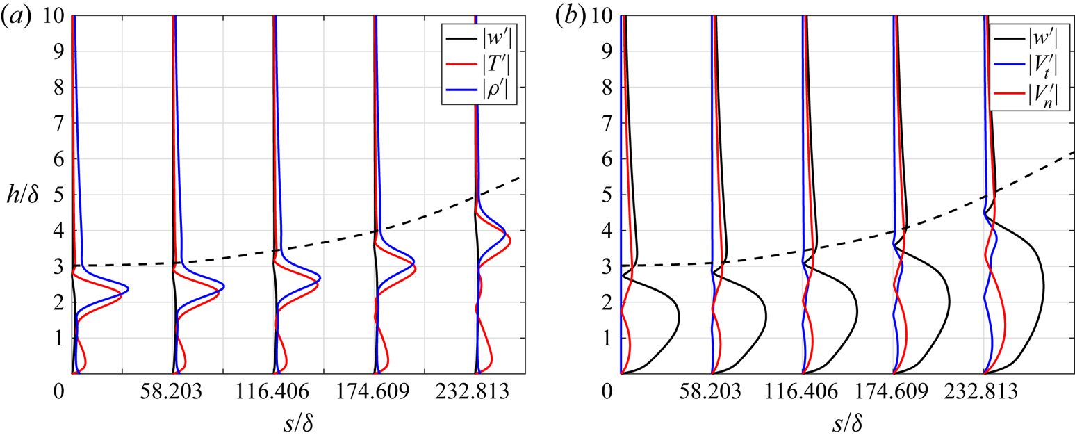
Figure 14. Perturbation profiles along the surface  $s$ direction at (from left to right)
  $s=0,58.203,116.406,174.609,232.813$ for C3376a case. (a) The perturbation profiles of spanwise velocity
  $|w'|$, temperature
  $|T'|$ and density
  $|\rho '|$. (b) The perturbation profiles of spanwise velocity
  $|w^{\prime }|$ surface tangential velocity
  $|V^{\prime }_t|$ and wall-normal velocity
  $|V^{\prime }_n|$. The dashed black lines represent the thickness of boundary layer
  $\delta ^{*}_{0.99}/\delta$.
To further analyse the spatial behaviour of perturbations, an energy norm  $E^{\prime }$ at specific
  $s$ is defined for the analysis of the leading boundary layer mode. The energy norm is defined as
 \begin{equation} E^{\prime} = \int_{h}(\boldsymbol{\phi}^{{\dagger}}\boldsymbol{M}\boldsymbol{\phi}) \, \textrm{d}h, \end{equation}
where  ${\boldsymbol {M}}$ is the energy weight matrix, the superscript
  ${\dagger}$ represents the conjugate transpose and
  $h$ the wall-normal distance. The weight matrix
  ${\boldsymbol {M}}$ was originally proposed by Mack (Reference Mack1984) and later independently derived by Hanifi, Schmid & Henningson (Reference Hanifi, Schmid and Henningson1996). It is defined as
 \begin{equation} \boldsymbol{M} = \text{diag}\left[\frac{T}{\gamma \rho M^2_{\infty}},\rho,\rho,\rho,\frac{\rho}{\gamma (\gamma - 1) T M^2_{\infty}} \right]. \end{equation}
According to the norm definition, both kinetic energy and the thermodynamic energy of the perturbations are taken into account. The energy norms for the four most dangerous cases are shown in figure 15. Ignoring the influence of the outflow region, this figure shows that the development of perturbations along the surface can be divided into three regions. For the leading-edge region  $s/R\in \left [0,0.12 \right ]$, as seen more clearly in the subfigure, the perturbations show, approximately, an exponential decay except for the case C3376a with
  $M_s=5.8$ which gives a typically algebraic growth at the region
  $s/R\in [0,0.06]$. Downstream at
  $s/R \in \left [0.12,1.3\right ]$ is a transition region before the third region
  $s/R \in \left [ 1.3, 1.57 \right ]$ where the perturbations grow exponentially.
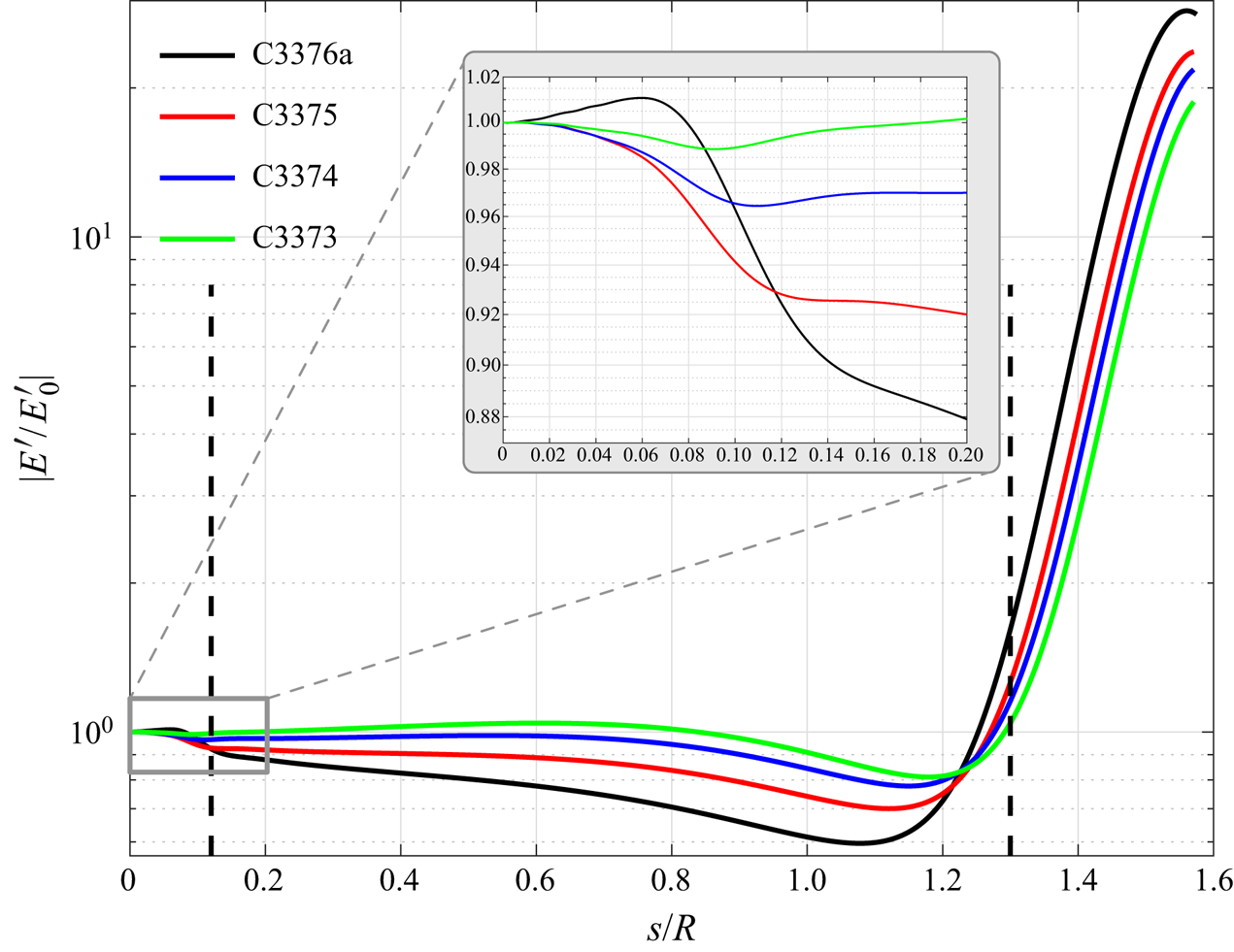
Figure 15. Variations of the energy norm  $|E^{\prime }|$ with respect to chordwise location
  $s/R$ for four cases. The energy norm is normalized with the energy
  $|E^{\prime }_0|$ at the attachment line (
 $s/R = 0$). The leading-edge region is enlarged for clarity.
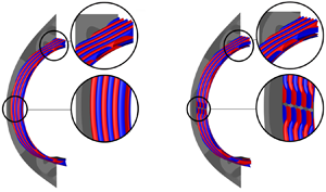
A three-dimensional visualization of the perturbation  $\boldsymbol {\phi }$ from the leading global eigenfunctions for C3376a case is illustrated in
  $\boldsymbol {\phi }_{3D}$ as
 \begin{equation} \boldsymbol{\phi}_{3D}(x,y,z) = \textrm{Re} [\boldsymbol{\phi}(x,y)(\cos(\beta z) + \textrm{i}\sin(\beta z))], \end{equation}
where  $\textrm {Re}(\lambda )$ represents the real part of a complex variable
  $\lambda$. The three-dimensional eigenfunctions
  $\boldsymbol {\phi }_{3D}$ are shown in figure 16(a,b). The typical symmetric and antisymmetric structures for spanwise and chordwise velocity perturbations (
 $W^{\prime }$ and
  $V_t^{\prime }$) can be observed by iso-surfaces and contours, as shown in figures 16(a), 16(b) and 16(d). From the figures, one can identified that from the leading edge (
 $s/R = 0$ in figure 16d) to further downstream (
 $|s/R| > 1.2$ in figure 16d) the leading global mode shows a transformation of locally two-dimensional instability to locally three-dimensional instability. At the leading edge around
  $y=0$, the eigenfunction has a spatial structure similar to the local attachment-line mode of sweep Hiemenz flow as first described by Lin & Malik (Reference Lin and Malik1996). Unlike incompressible cases, the counter-rotating vortices are somewhat further away from the surface as shown in figure 16(c). The vortices generate chordwise velocity streaks and similar features are identified by Mack et al. (Reference Mack, Schmid and Sesterhenn2008) for parabolic leading-edge flow at relatively low sweep Mach numbers over an adiabatic surface. Further downstream, the three-dimensional instability is reflected by the obvious distortions of the iso-surface as enlarged in figure 16(a,b). The contours of
  $n$–
$n$– $z$ planes for the spanwise velocity and density are also shown in figure 17 and the second Mack-mode-like features of this global mode is found to become more prominent further downstream.
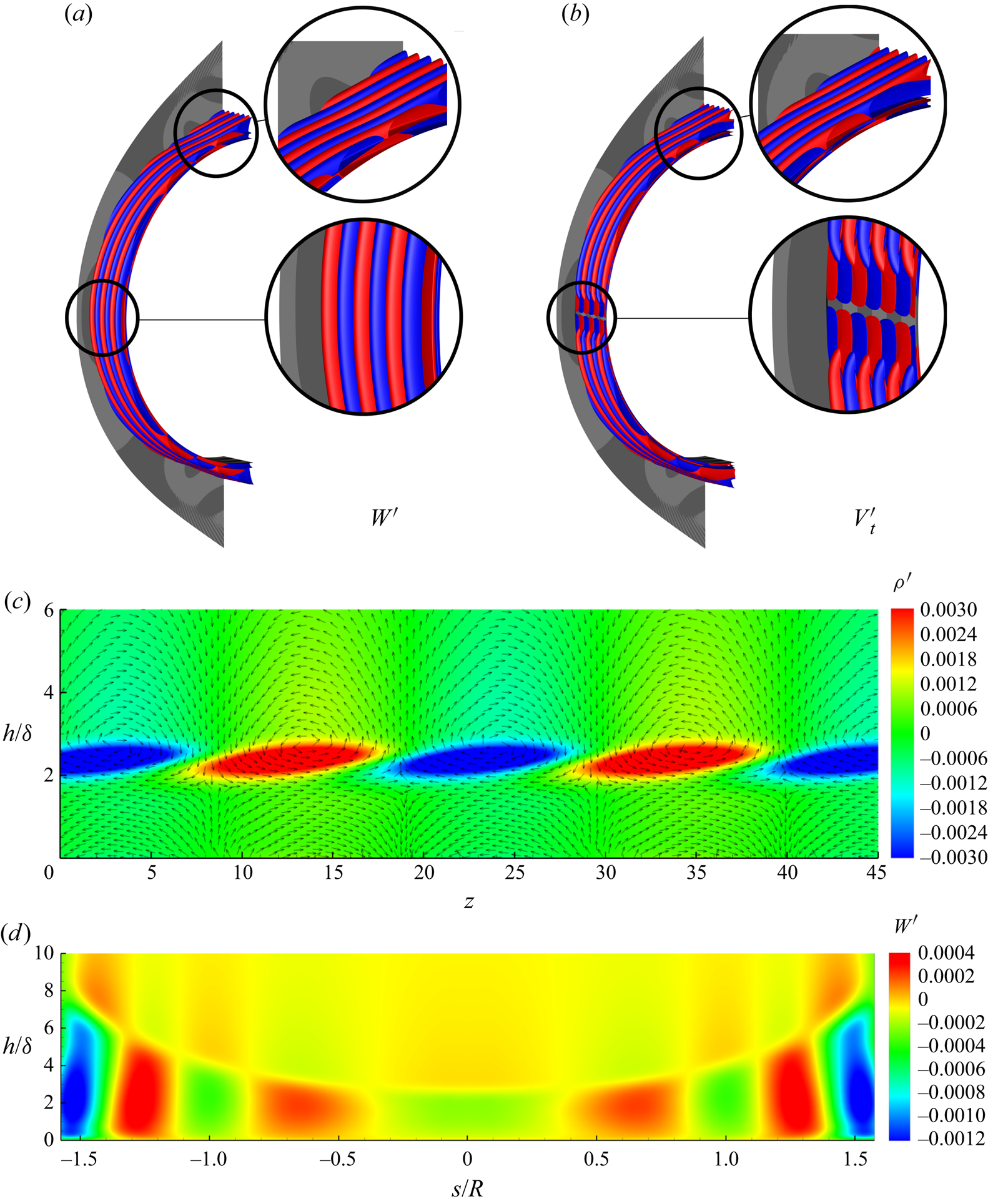
Figure 16. The leading global modes of the eigenvalue  $\omega = (0.25097, 0.00073146)$ visualized by iso-surfaces (positive value in red, negative value in blue) of (a) the spanwise velocity perturbation
  $W^{\prime }(x,y,z) = \textrm {Re}({w^{\prime }(x,y)(\cos \beta z + \text {i}\sin \beta z )})$ at contour level of
  $\pm 10^{-5}$ and (b) the surface tangential velocity perturbations at contour level of
  $\pm 10^{-6}$, contours of the relative density perturbation are also shown at the background. (c) Contour of the
  $x$–
$x$– $z$ plane cross-cut at
  $y=0$ for density perturbation
  $\rho ^{\prime }(x,y,z)$ together with the velocity vector (unit vector) on this plane. (d) Contour of the spanwise velocity perturbation
  $W^{\prime }$ on the
  $s$–
$s$– $n$ plane at
  $z=0$.
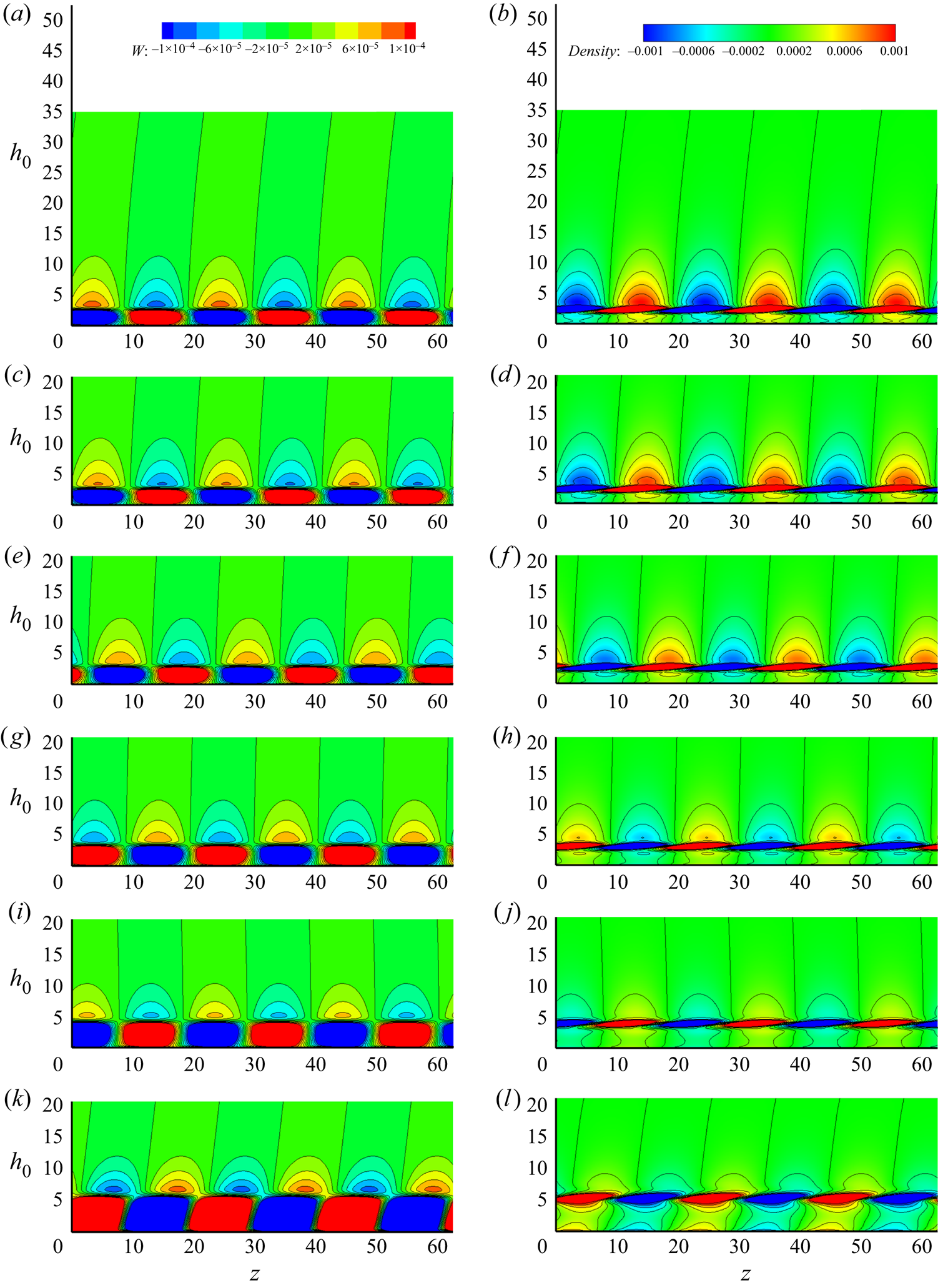
Figure 17. Contours of spanwise perturbation  $w'$, left-hand side column, and density perturbation
  $\rho '$, right-hand side column, of
  $n$–
$n$– $z$ plane along surface
  $s$ direction at (from the top down)
  $s=0,58.2,116.4,174.6,232.8$ and
  $291.0$. Here
  $h_0$ represents the distance away from surface.
To have a better understanding of the mechanism behind the mode and the obvious energy growth as presented in figure 15, we perform the following analyses for the C3376a case. Following the study of Malik, Li & Chang (Reference Malik, Li and Chang1994), we define the cross-flow velocity  $U_c$ related to the inviscid flow direction outside of the boundary layer. The cross-flow Reynolds number
  $Re_{cf}$ is defined as
 \begin{equation} Re_{cf} = \frac{U_c^{max} \delta}{\nu_r}. \end{equation}
Here  $U_c^{max}$ is the maximum cross-flow velocity inside the boundary layer. Figure 18 shows the cross-flow velocity profiles along the surface from the attachment line to the exit of the computational domain. As the boundary develops under the pressure gradient (as shown in figure 7), the components of cross-flow increase gradually and the relative cross-flow Reynolds number increases from
  $0$ (at attachment line plane) to
  $204.13$ (at exit plane). At the same frequency (
 $\omega = 0.25097$) of the global calculation (in figure 12), we perform spatial local linear stability analyses over the cylinder surface based on the NS solution. In contrast to the previous linear stability analyses, we perform locally quasi-parallel analysis, based on another normal mode ansatz,
 \begin{equation} \boldsymbol{\varPhi}(s,n,z,t) = \boldsymbol{\phi}(n)\exp \left(\textrm{i}\alpha_s s + \textrm{i}\beta z - \textrm{i}\omega t\right) + \textrm{c.c.}, \end{equation}
in which  $\beta$ and
  $\omega$ are the same as previous definitions. We solve the eigenvalue
  $\alpha _s$, the wave number and growth rate along the chordwise direction. The stability diagram of the given frequency is shown in figure 19(a). The small region around the leading edge (
 $s/R\in \left [0,0.2\right ]$) from this local calculation is non-physical because of non-ignorable variations of mean flow at
  $s$ direction. The horizontal dashed line represents the same spanwise wave numbers as in global calculation, and the growth rate (
 $-\alpha _{si}$) along this line is shown in figure 19(b). Moreover, the behaviour of the mode calculated from local calculation agrees well with those from the global calculation as compared with figure 15. The rapid energy increase started at around
  $s/R = 1.2$ in figure 15 is reflected directly as the unstable downstream region shown in figure 19(b). In addition, figure 19(a) shows that the unstable region is made up of three parts. To identify the features in those regions, three eigenfunctions corresponding to circles marked in figure 19(a) are shown in figures 19(c), 19(d) and 19(e). Good agreement of the eigenfunctions, marked in region III, from the local spatial calculation and global temporal analysis can be observed in figure 19(e). The physical frequency of the perturbation
 \begin{equation} f = {\omega |{\boldsymbol{V}}_{\infty}|}/{2{\rm \pi} \delta}, \end{equation}
predicted by previous global analyses is  $311\ \text {kHz}$ and is located in the region of the second Mack mode. The locations of the critical layer (
 $c_r = \bar {U}$) and the sonic lines (
 $c_r = \bar {U} + a$), where
 \begin{equation} c_r = \frac{\omega}{\sqrt{\alpha_s^2 + \beta^2}},\quad \bar{U} = \frac{\alpha_s U + \beta W}{ \sqrt{\alpha_s^2 + \beta^2}},\quad a = \frac{\sqrt{T}}{M_{\infty}}, \end{equation}
are shown in figures 19(c), 19(d) and 19(e). From figure 19(e), we can find that the majority of the perturbations lies below the sonic line with only the temperature and density peak near the critical layer, which is the typical feature of the second mode (Hader & Fasel Reference Hader and Fasel2019; Paredes, Choudhari & Li Reference Paredes, Choudhari and Li2020). All these indicate that the instability at region III and the rapid energy increase started at around  $s/R = 1.2$ in figure 15 is due to the second Mack mode.

Figure 18. The cross-flow velocity profiles along the surface  $s$ of the cylinder at (from left to right)
  $s=43.53$, 87.06, 130.59, 174.12, 217.65, 261.18, 304.71 and
  $347.04$ for the C3376a case.
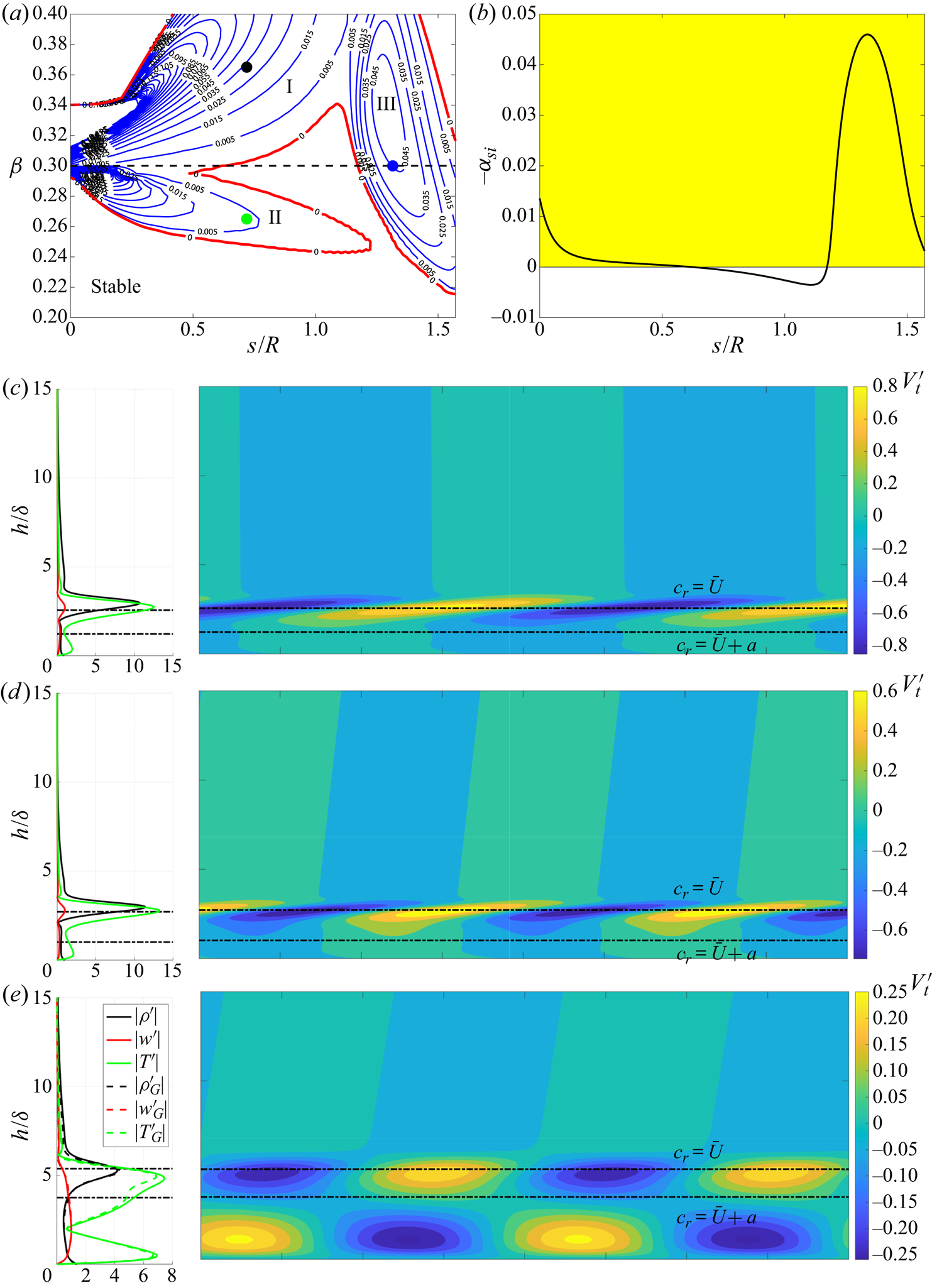
Figure 19. (a) The stability diagram of the C3376a case based on local stability analysis. The frequency is such chosen that matches the leading unstable global mode. The horizontal dashed line represents the spanwise wave number  $\beta = 0.3$ as in the global calculation. The growth rate
  $-\alpha _{si}$ along the dashed line is shown in (b). The points marked by black, green and blue, in three regions I, II and III, are shown with eigenfunctions in (c), (d) and (e), respectively. Left parts of these panels show the perturbation profiles for density
  $|\rho ^{\prime }|$, spanwise velocity
  $|w^{\prime }|$ and temperature
  $|T^{\prime }|$, all normalized with maximum spanwise velocity perturbation. The global eigenfunction
  $(|\rho ^{\prime }_{G}|, |w^{\prime }_{G}|,|T^{\prime }_{G}|)$ is also shown in (e) for comparison. Right parts of (c), (d) and (e) show the corresponding chordwise velocity
  $|V^{\prime }_t|$. The locations of the critical layer
  $c_r = \bar {U}$ and the sonic lines
  $c_r = \bar {U} + a$ are indicated by horizontal dash-dotted lines.
Regions I and II, on the other hand, support similar perturbation profiles as presented in figures 19(c) and 19(d). To recognize the feature of these two parts and the instability nature, we further show the stability diagram at lower frequencies in figure 20. For stationary case ( $f = 0\ \textrm {kHz}$), shown in figure 20(a), the typical neutral curves for stationary cross-flow instability is shown. When the frequency goes higher (
 $f = 24.78\ \textrm {kHz}, 49.567\ \textrm {kHz}$), the unstable region moves up covering higher spanwise wave numbers, as shown in figure 20(b,c). Owing to the continuous change of the stability diagram, the instability there is identified as travelling cross-flow instability. As the frequency further increases, not only does the cross-flow region go to a higher spanwise wave number region, but another unstable region appears in the lower spanwise wave numbers, as presented in figures 20(d), 20(e) and 20(f). We term instabilities in this region as mode II in this study. At higher frequencies, the region of the second mode appears (figure 20g,h) and forms the final neutral curve shown in figure 19(a), in which the frequency reaches the value predicted by global calculation. Therefore, based on the stability features along the dashed line in figure 19 and global analyses, the dominating perturbations display the features of attachment-line modes at the leading edge, a combination of the mode II instability and travelling cross-flow instability just downstream and the features of the second mode instability further downstream.
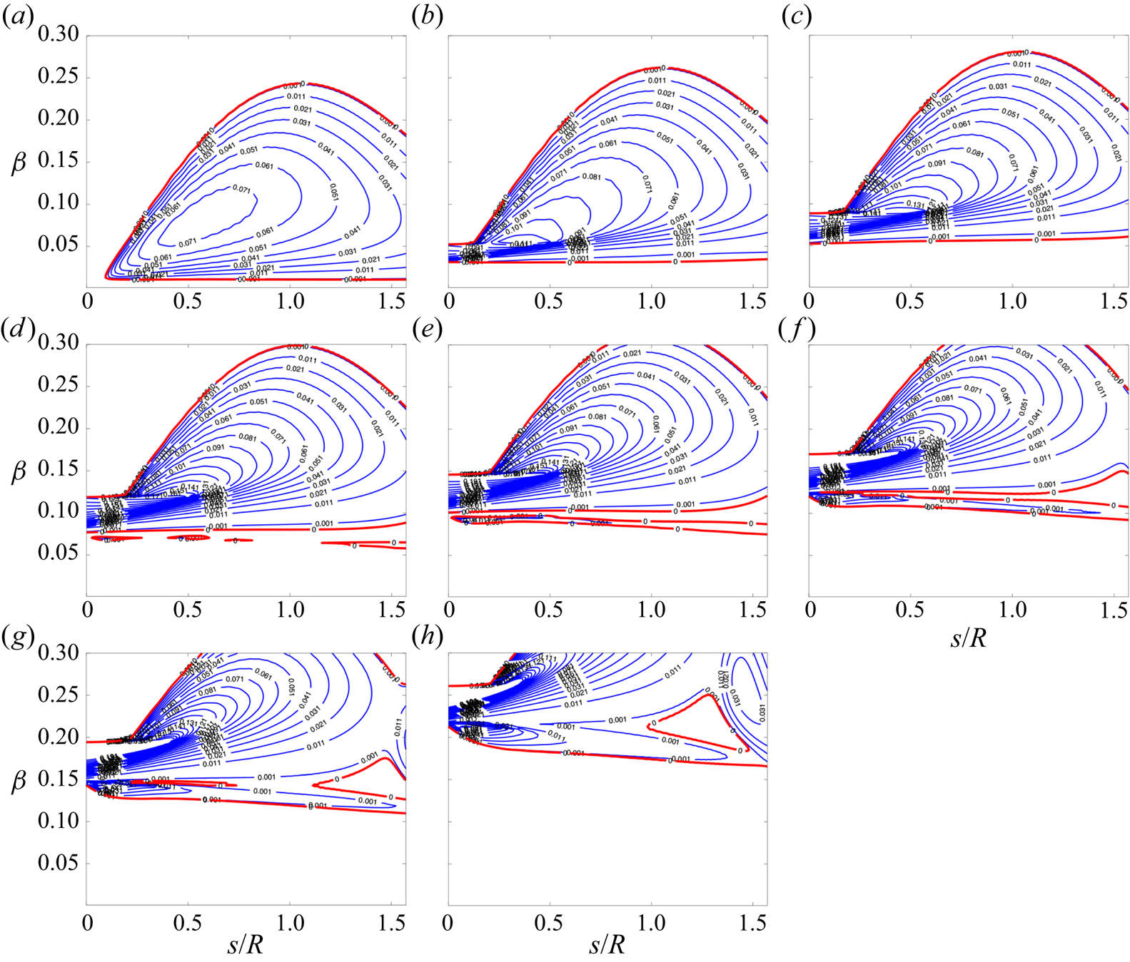
Figure 20. Stability diagrams of the C3376a case at different frequencies (a) 0.00 kHz, (b)  $24.784\ \text {kHz}$, (c)
  $49.567\ \text {kHz}$, (d)
  $74.351\ \text {kHz}$, (e)
  $99.135\ \text {kHz}$, (f)
  $123.92\ \text {kHz}$,
  $(g)$
$(g)$  $148.70\ \text {kHz}$ and (h)
  $223.05\ \text {kHz}$.
4.1. Lower sweep Mach number cases
Additional cases are calculated to capture the instability features varying with sweep Mach numbers over a larger range. In this study, we still alter the sweep angle as we did previously to cover the regions of relatively lower sweep Mach numbers. The additional cases are listed in table 3. All the parameters are the same as previous except for the sweep angle  $\varLambda$ and surface temperature
  $T_w$. As there is no experimental data for these configurations, an adiabatic surface temperature
  $T_w = T_r$ will be analysed for these cases. In fact, the cold surface cases
  $T_w < T_r$ are also calculated for these cases, not only did not we find the unstable modes, but the leading attachment-line mode is absorbed into the continuous spectrum and can hardly be identified. For these reasons, the cold wall cases are not shown here. For this model, as the sweep angle
  $\varLambda$ increases from
  $25$ to
  $55^{\circ }$,
  $Re_s$ rises from around 500 to 1000, exhibiting a different tendency as compared with high sweep angle cases as presented in table 1. After solving the basic flow with high-order shock fitting methods, we perform the global stability analyses focusing on the attachment-line instability.
Table 3. Parameters for additional cases.
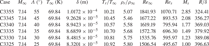
The basic flow and attachment-line perturbations for C3335 case are shown in figure 21. The typical feature of an adiabatic boundary layer is presented in figure 21(a). Two generalized inflection points are also found close to the wall surface. The eigenfunctions at the attachment line calculated by global stability solver are shown in figure 21(b) and exhibit characteristics of TS instability, comparing with previous studies (Lin & Malik Reference Lin and Malik1995; Gennaro et al. Reference Gennaro, Rodríguez, Medeiros and Theofilis2013).
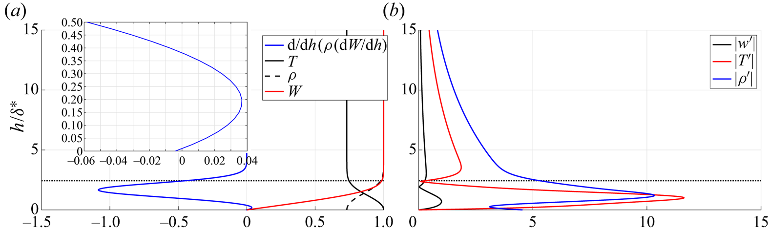
Figure 21. (a) The basic flow profiles at the attachment line. The density  $\rho$ and spanwise velocity
  $w$ are normalized by the reference value at the edge of stagnation boundary layer. The temperature is normalized by the recovery temperature
  $T_r$. The small region of
  ${\textrm {d}}/{\textrm {d}h}(\rho ({\textrm {d}W}/{\textrm {d}h}))$ near the surface is enlarged and presented on the top left. (b) The perturbations of the leading attachment-line mode. All the perturbations are normalized with the maximum spanwise velocity. The horizontal dotted lines represent the edge of the boundary layer.
The calculated spectrum for spanwise wave number  $\beta = 0.19$ is shown in figure 22(a). The branch of attachment line instability is marked by black, filled dots. Similar to the incompressible cases (Lin & Malik Reference Lin and Malik1996, Reference Lin and Malik1997), symmetric (
 $S1,S2,\ldots$) and antisymmetric (
 $A1,\ldots$) eigenvalues alternate from the least stable to the most stable. Typical features are shown in details through the iso-surfaces of spanwise velocity perturbations for
  $S1$ and
  $A1$ modes, as presented in figure 22(c,d). Dependences of eigenvalues
  $\omega _i$ on
  $\beta$ for the least stable symmetric
  $S1$ and antisymmetric
  $A1$ modes is shown in figure 22(b). In this region, it is found that all these modes are stable among which the symmetric mode
  $S1$ always has the highest growth rate.
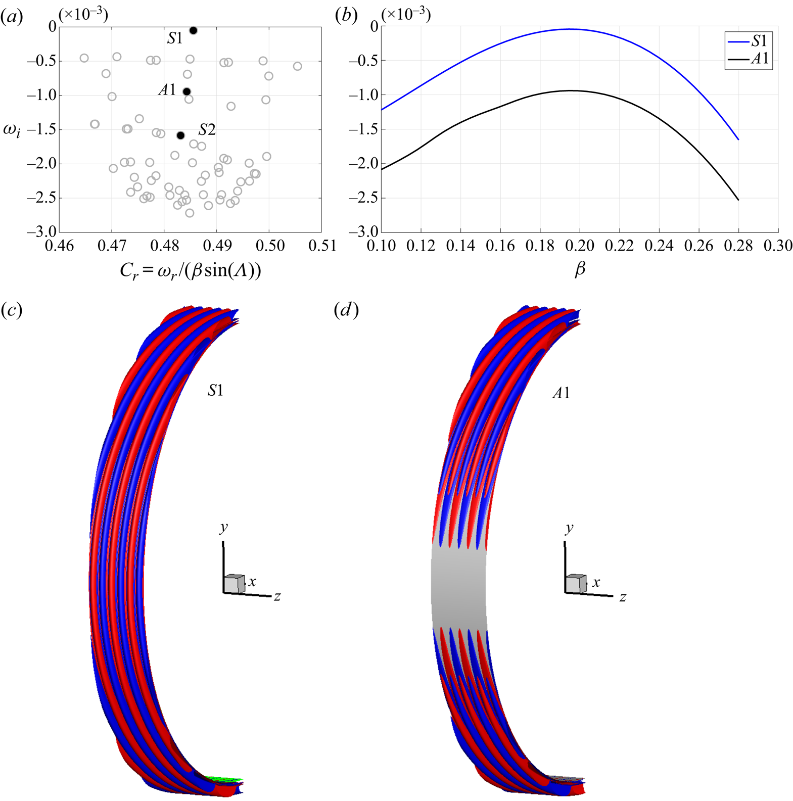
Figure 22. (a) Eigenvalues of the C3335 cases for spanwise wave number  $\beta = 0.19$. The branch of attachment-line modes is marked by black, filled dots. Symmetric (
 $S1,S2,\ldots$) and antisymmetric (
 $A1,\ldots$) eigenvalues alternate from the least stable to the most stable. Here
  $S1$ and
  $A1$ modes are visualized by iso-surface of the spanwise velocity perturbation at contour level of
  $\pm 10 ^{-5}$ in (c,d), respectively. (b) Dependences of
  $\omega _i$ on
  $\beta$ for
  $S1$ and
  $A1$ modes for C3335 case.
The dependences of growth rates to the spanwise wavelength of the perturbations for additional cases are shown in figure 23, except for C3355 case because some of the attachment-line modes in that cases are so close to the continuous branches and cannot be identified in global calculations. Obviously, all the attachment-line mode is stable. As the sweep angle increases from  $25$ to
  $45^{\circ }$, the maximum growth rates show a trend from rising to decline, reaching the highest points between
  $35$ and
  $40^{\circ }$.
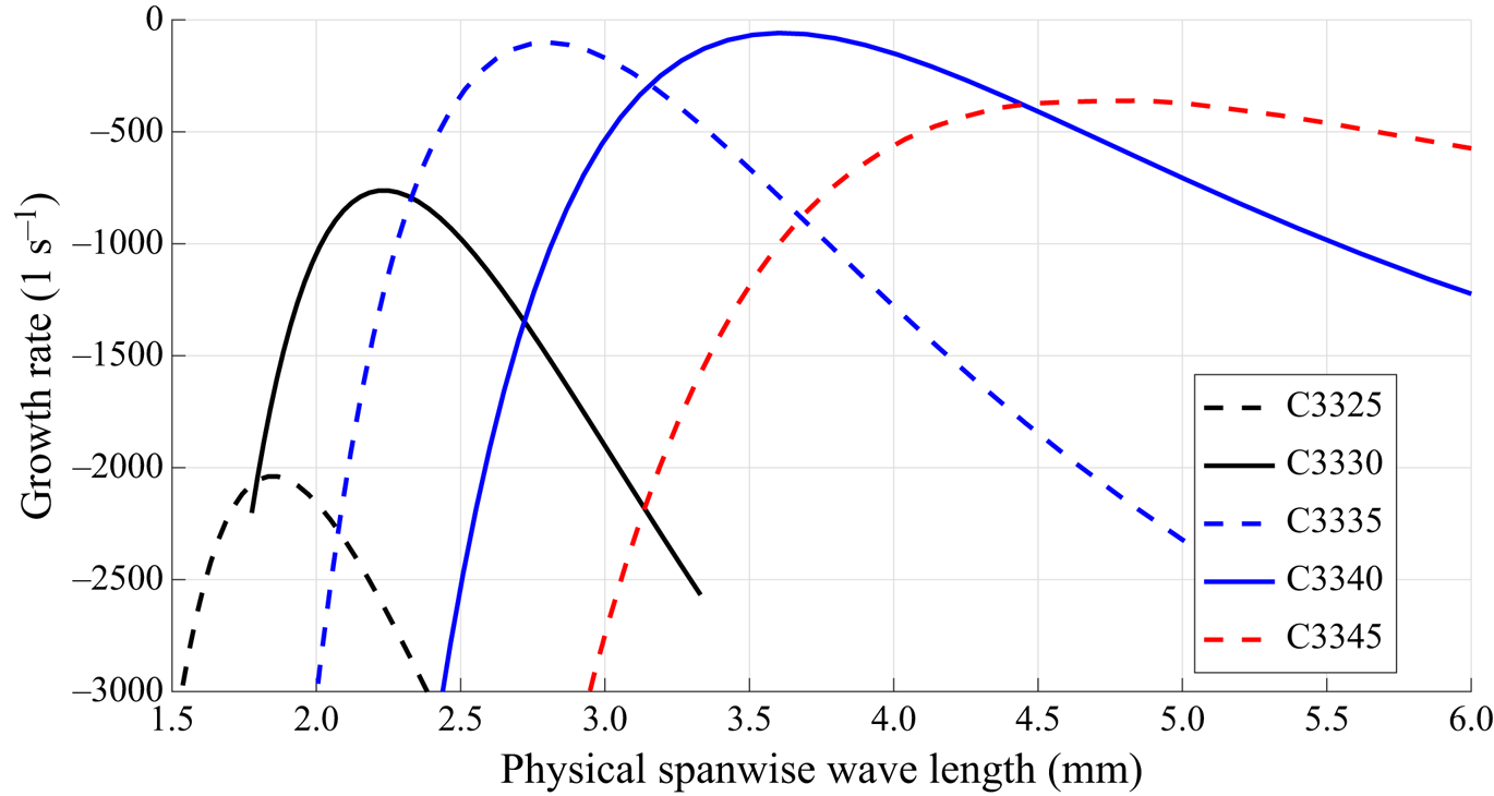
Figure 23. Dependences of physical growth rates on the physical spanwise wavelengths of perturbations in the small sweep angle regime.
5. Concluding remarks
The present work attempts to explain, theoretically, the instabilities of attachment line at high sweep Mach numbers in accordance with relevant experimental conditions (Gaillard et al. Reference Gaillard, Benard and Alziary de Roquefort1999). The analysis is performed with high-fidelity realistic basic flows which are obtained with a high-order shock fitting method to fully resolve the basic flow and all the geometry information. Local and global stability analyses are employed to elucidate the physics of the attachment-line instability. The theoretical results agree qualitatively with the experiment. This type of attachment-line mode is found belonging to the inviscid instability and locate in the frequency range of the second Mack mode, in contrast to the low-speed cases which belong to the viscous instability. From the global stability analysis, the leading attachment-line mode is found to be connected with the second Mack modes further away from the attachment line.
An exploration into the lower sweep Mach number regime connects the present findings to those reported in the smaller  $M_s$ regime. When the sweep angle increases from 0, the attachment-line mode gets promoted until 35–
 $40^{\circ }$. This is followed by a suppression until the large
  $M_s$ regime (with sweep angle from 65 to
  $76.5^{\circ }$) where the instability become substantially enhanced, as shown in figure 24.
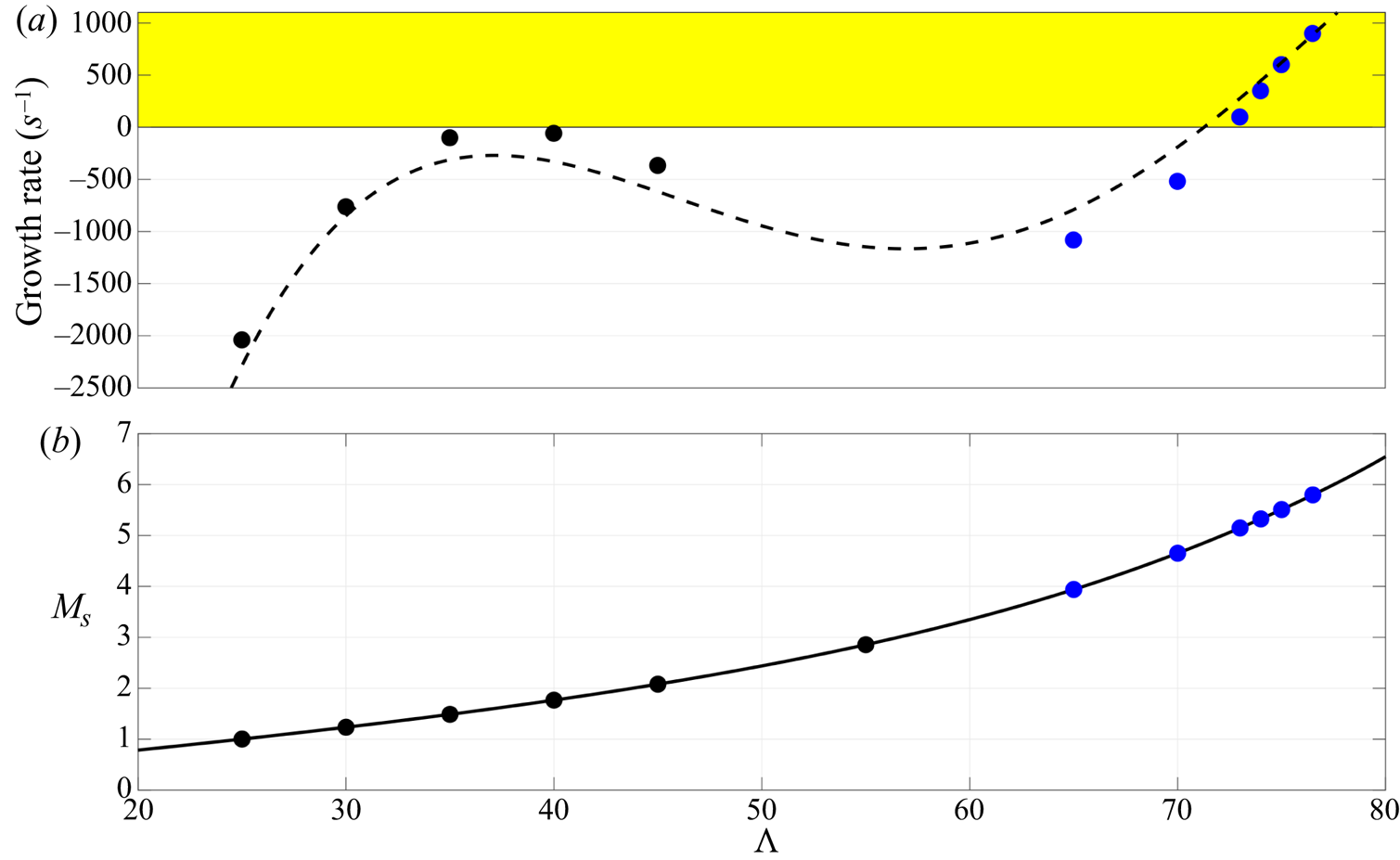
Figure 24. The anticipated behaviour of the leading attachment-line mode for a hypersonic blunt sweep body on different sweep angles  $\varLambda$ and sweep Mach numbers
  $M_s$. The dashed line represents the predicted growth rate for a typical configuration of hypersonic sweep body. The black and blue filled dots represent the maximum growth rate for the cases calculated in the present analyses.
It is also found that the more realistic basic flow is the key to understanding some unexplained phenomenon. The traditional boundary layer model fails to take the influence of inviscid flow into consideration, and this influence sometimes may change the physics of flow instability significantly as in this case. Based on the inviscid nature of attachment-line mode found in this study, a mode competition/transformation between inviscid and viscous attachment-line modes may occur at specific parameter region, especially for lower sweep Mach number over a cold wall. In addition, the inner relationship between attachment-line modes and unsteady cross-flow modes in the high-Mach-number region is still unclear. In some study (Mack et al. Reference Mack, Schmid and Sesterhenn2008), the attachment-line instabilities in the leading-edge region connect with cross-flow modes further away from the leading edge. In contrast, these connections may disappear in some other cases as pointed out by Paredes et al. (Reference Paredes, Gosse, Theofilis and Kimmel2016). The study on these aspects may be important extensions of the present research.
Acknowledgements
Useful discussions with Dr Z. Wang, Professor Q. Li of Tsinghua University and Dr J. Liu of Tianjin University are gratefully acknowledged. We appreciate Professors R. Paciorri, A. Bonfiglioli and X. Zhong for useful discussion on shock-fitting method. Conversations with Dr P. Paredes and Professor V. Theofilis on the global stability method are also helpful.
Funding
This work received partial support from the National Key Project GJXM92579, NSFC Grants 11602127 and 11572176 and National Science and Technology Major Project (2017-II-0004-0016).
Declaration of interests
The authors report no conflict of interest.
Appendix A. Verification and validation of the shock-fitting and boundary layer solver
Three cases were used to check our code. Two cases (the hypersonic flow over a cylinder and a parabola) calculated by Zhong (Reference Zhong1998) are used for validation and verification of the present solver. Excellent agreements are achieved as shown in figures 25 and 26 for pressure coefficient and vorticities. The last one comes from DNS study of Balakumar & King (Reference Balakumar and King2012) (a supersonic flow over a sweep cylinder), we had used an inviscid shock-fitting Euler solution together with a boundary layer equation to solve the problem. Again, in figure 27 the density profiles at several stations match perfectly.
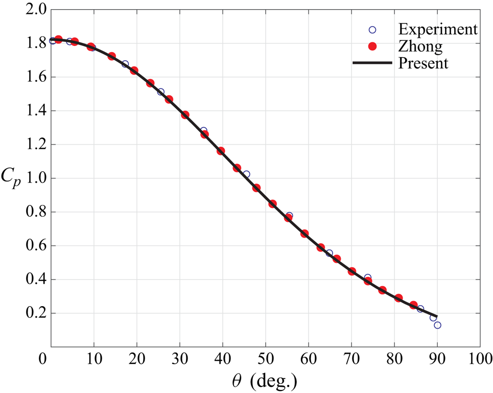
Figure 25. Dependence of  $C_p$ on
  $\theta$ for a flow around cylinder at Mach
  $5.73$. The line represents the solution calculated with the authors’ code. The circles represent results from Zhong (Reference Zhong1998) and experiment (Tewfik & Giedt Reference Tewfik and Giedt1960).
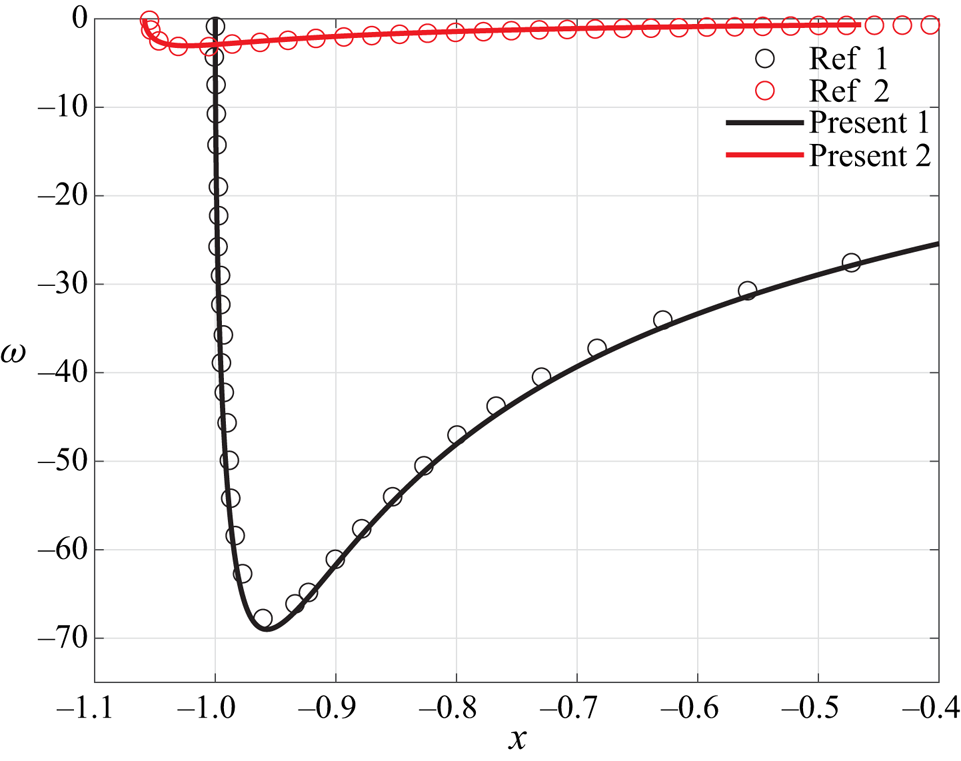
Figure 26. Dependence of vorticity  $\omega$ behind the shock surface and over the wall surface over a hypersonic blunt parabola at Mach
  $15$. The lines are from the solution calculated with the authors’ code. The circles marked as Ref 1 and Ref 2 represent results from Zhong (Reference Zhong1998).
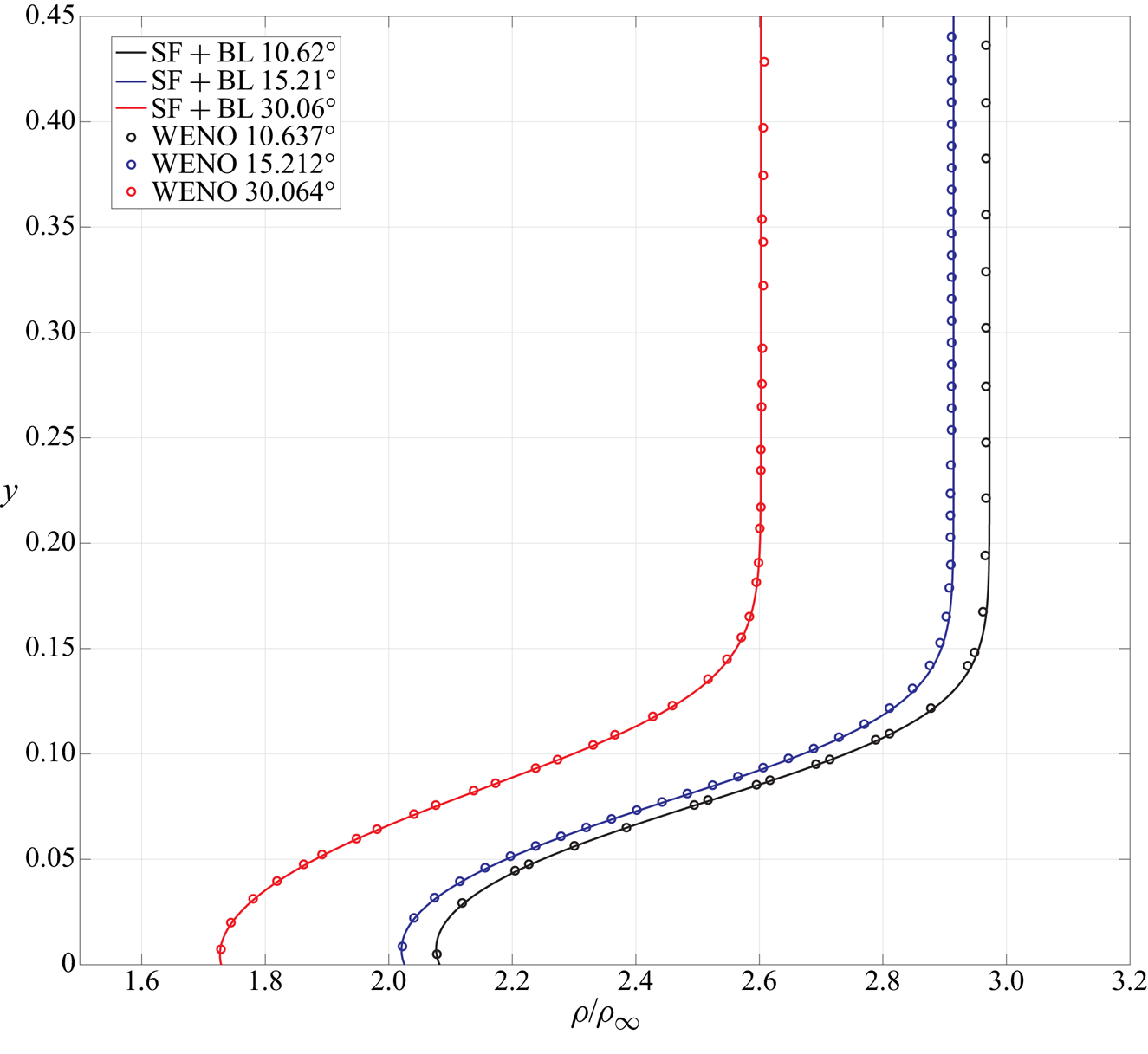
Figure 27. Comparison of the density profile at several station over a sweep cylinder at Mach 3. The lines represent the solution calculated with the authors’ code. The circles represent the solution calculated by the weighted essentially non-oscillatory (WENO) scheme from Balakumar & King (Reference Balakumar and King2012).
Appendix B. Verification and validation of the global stability solver
Two types of cases have been used to validate the global stability solver developed in this work. First, the linear stability of the incompressible and subsonic sweep attachment-line flow is addressed here to check the reliability and accuracy of the solver with the results from the literature (Theofilis et al. Reference Theofilis, Fedorov and Collis2006; Gennaro et al. Reference Gennaro, Rodríguez, Medeiros and Theofilis2013). The dependence of the scaled eigenvalues  $C = \omega /\beta$ on
  $\beta$ is shown in figure 28 and these eigenvalues represents the G–H mode of the boundary layer. The boundary conditions in the present simulation remain the same as in the literature.
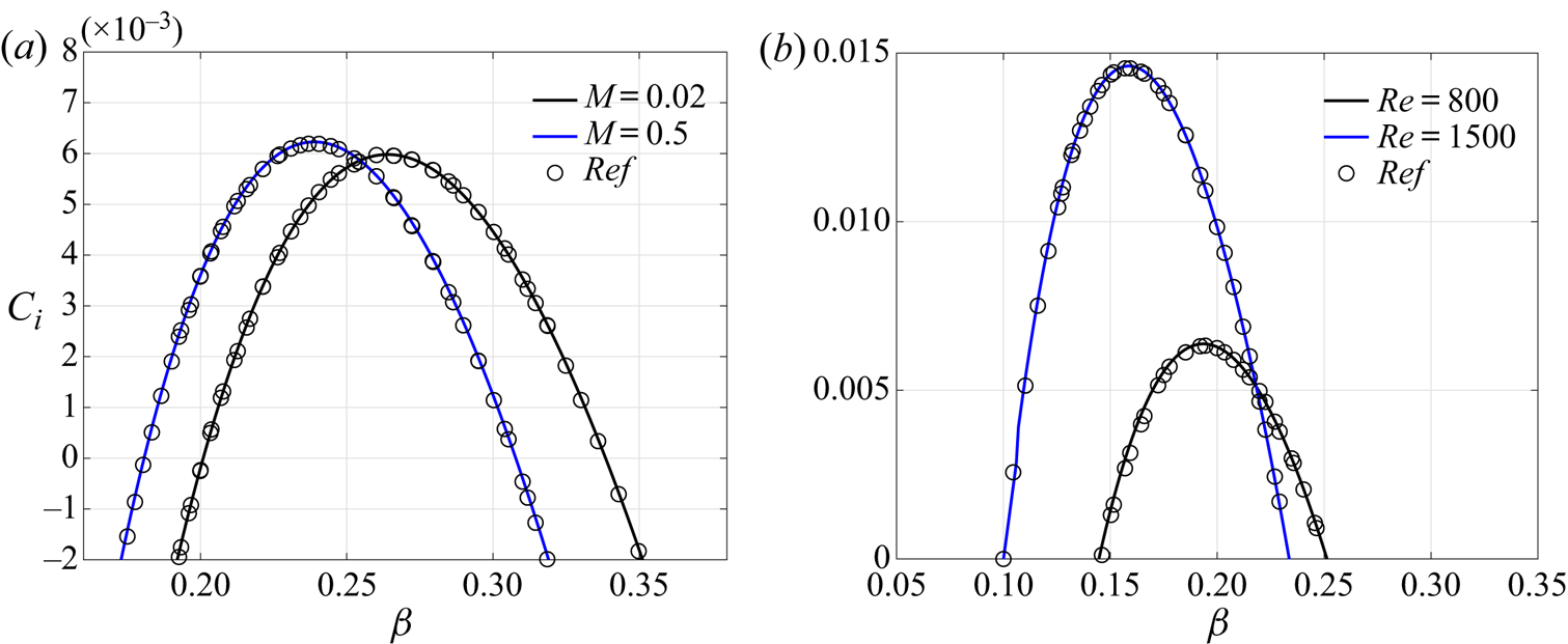
Figure 28. (a) Dependence of  $C_i$ on
  $\beta$ for G–H mode at
  $Re=800$. (b) Dependence of
  $C_i$ on
  $\beta$ for G–H mode at
  $M=0.9$. The data obtained by asymptotic analysis (circle) and results of the present study (solid line). In this test case, we use
  $121\times 121$ grid points and the problem is discretized with eighth-order finite difference method.
Then the solver is also compared with the local stability solver on high-speed two-dimensional boundary layer cases. The spatial version of this solver is used and compared with previous studies. Balakumar & Malik (Reference Balakumar and Malik1992) reported an eigenvalue  $\alpha =0.220-0.003091{i}$ for a high-speed boundary layer and the present bi-global solver obtains
  $\alpha =0.220199-0.003098{i}$. In addition, for a high-speed boundary layer, Tumin (Reference Tumin2007) reported an eigenvalue
  $\alpha =0.2534420-0.0027738{i}$, and the present solver achieved
  $\alpha =0.253442-0.002780{i}$. These cases are listed and compared in table 4. The matches, listed in table 4 and shown in figure 28, demonstrate the reliability and numerical accuracy of the newly developed solver.
Table 4. High-speed boundary layer validation cases. For case 1, the parameters are as follows: the free-stream Mach number  $M=4.5$, the total temperature
  $T_0=311\ \textrm {K}$, the Prandtl number
  $Pr=0.72$, the Reynolds number
  $Re=1000$ and the frequency
  $\omega =0.2$. For case 2, the parameters are as follows. The free-stream Mach number
  $M=4.5$, the total temperature
  $T_0=611.11\ \textrm {K}$, the Prandtl number
  $Pr=0.70$, the Reynolds number
  $Re=1500$ and the frequency
  $\omega =0.23$. In both cases,
  $121\times 120$ grid points are used with an eighth-order finite difference method.
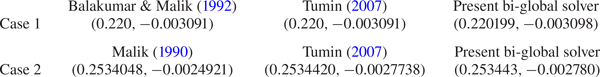
Appendix C. Basic flow solution based on boundary layer approximation
First, an Euler system is solved with the shock fitting method to provide the boundary information for boundary layer equations. Detailed information on boundary conditions for Euler equations can be found in Brooks & Powers (Reference Brooks and Powers2004). Then the boundary layer equations are solved along the surface as in Wang et al. (Reference Wang, Wang, Wang, Xu and Fu2018). We take the C3376a case as a typical example and other cases have similar features. At the attachment line, the profiles for variables are shown in figure 29 together with the solution from full NS calculation. Further downstream the profiles are also shown and compared in figure 30.
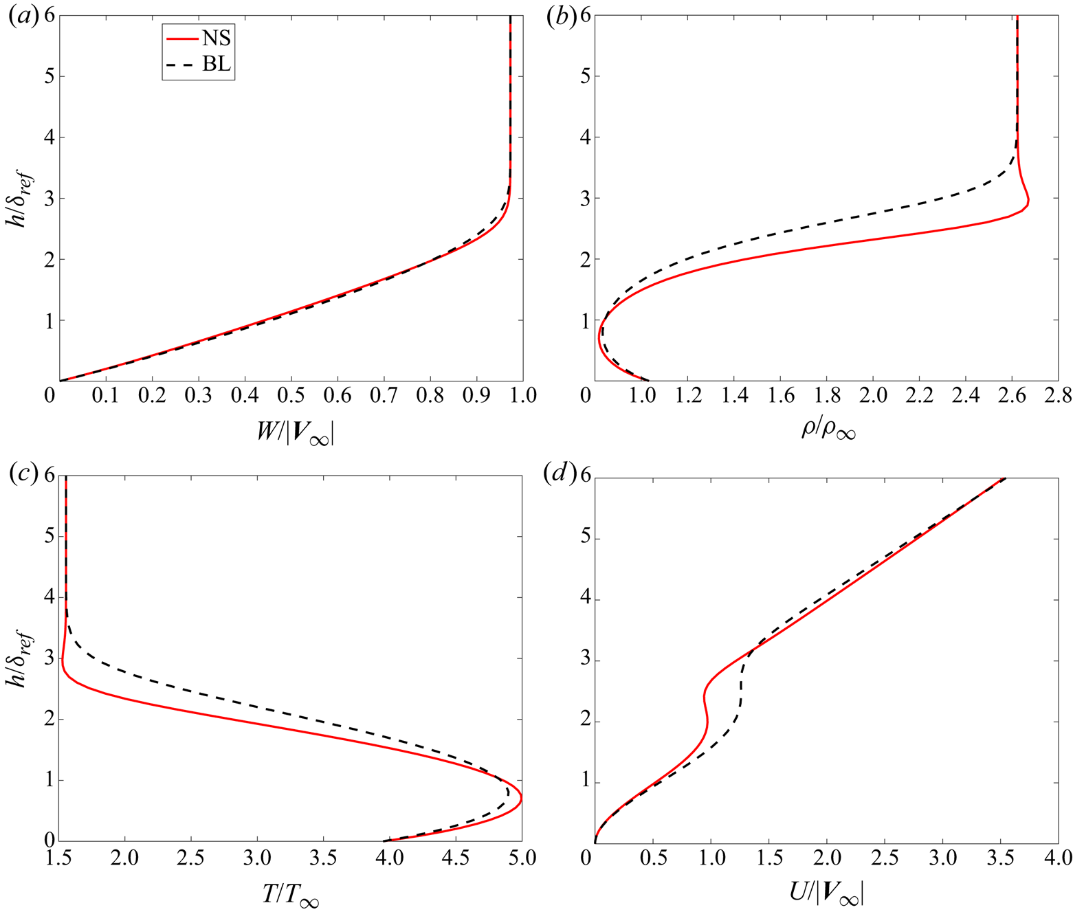
Figure 29. The variable profiles at the attachment line. All the variables are normalized with the free-stream values. Velocity is normalized with the free-stream velocity  $|{\boldsymbol {V}}_{\infty }|$. The red line represents the solution from full NS calculation and the dashed black line is from boundary layer approximation.
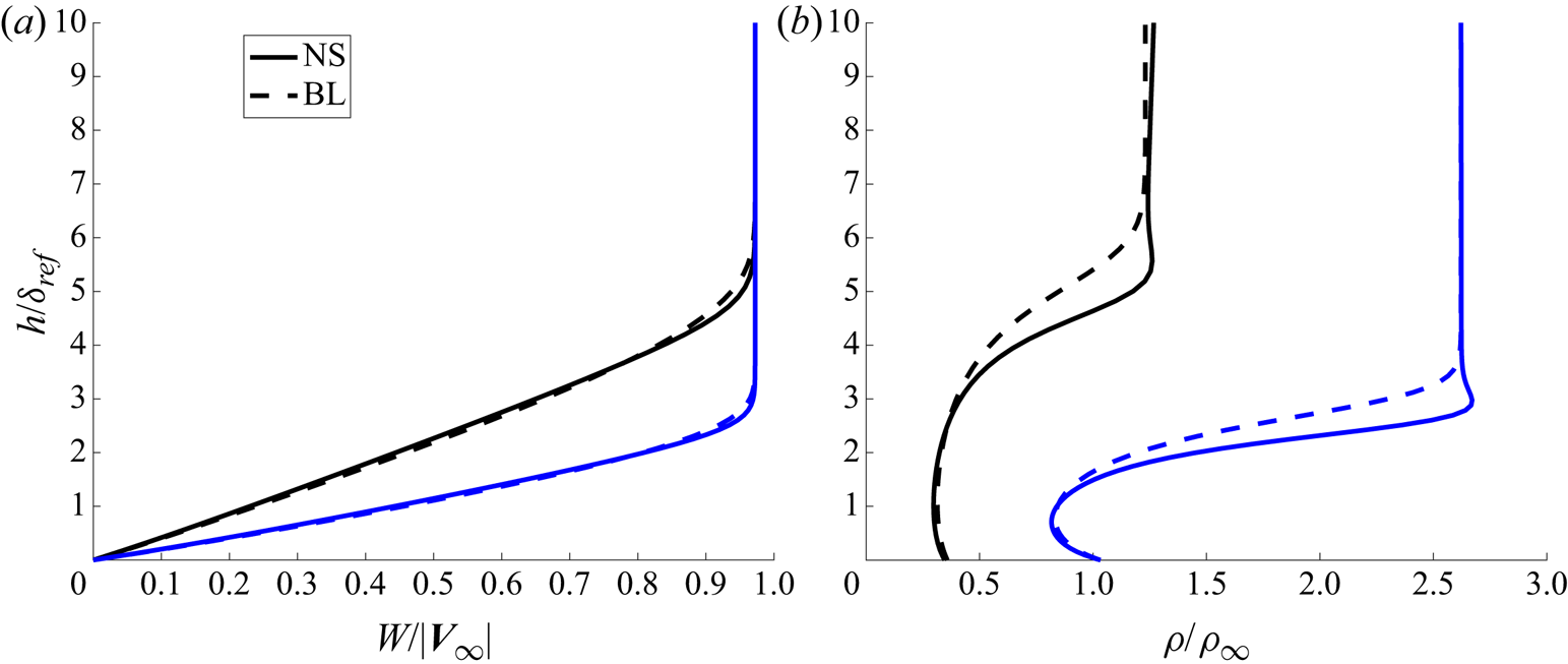
Figure 30. The variable profiles at two different surface locations: (a) the spanwise velocity and (b) the density. The lines represent the solution from full NS calculation and the dashed lines are from boundary layer approximation. The blue line is located at  $s = 0$ and the black line is located at
  $s = 1.18R$.
Appendix D.  $O(1)$ equation along the attachment line

A small parameter  $\epsilon = 1/Re$ and slow variables
  $y_1 = \epsilon y, t_1 = \epsilon t$ are introduced. In the framework of multiple-scale approach, the perturbation is expressed as
 \begin{equation} \varPhi(x,y,z,t) =\varphi_n\exp\left[\textrm{i}\beta z - \textrm{i}\omega t\right], \end{equation}
where
 \begin{equation} \varphi_n=\phi_0(x,y_1,t_1) + \epsilon \phi_1(x,y_1,t_1) + \epsilon^2 \phi_2(x,y_1,t_1) + O(\epsilon^3) + \cdots. \end{equation}
Substituting (D1) into the LNS equations, the equations for  $O(1)$ can be expressed as
 \begin{equation} {-}\textrm{i} \omega {\boldsymbol{\varGamma}} \phi_0 + \boldsymbol{A}\frac{\partial \phi_0}{\partial x} + \textrm{i}\beta \boldsymbol{C} \phi_0 + \boldsymbol{D}\phi_0 - \boldsymbol{H}_{xx}\frac{\partial^2 \phi_0}{\partial x^2} - \textrm{i} \beta \boldsymbol{H}_{xz}\frac{\partial \phi_0}{\partial x} + \beta^2 \boldsymbol{H}_{zz}\phi_0 = 0, \end{equation}
and  $O(\epsilon )$ as
 \begin{align} &-\textrm{i} \omega \boldsymbol{{\varGamma}} \phi_1 + \boldsymbol{A}\frac{\partial \phi_1}{\partial x} + \textrm{i}\beta \boldsymbol{C} \phi_1 + \boldsymbol{D}\phi_1 -\boldsymbol{H}_{xx}\frac{\partial^2 \phi_1}{\partial x^2} - \textrm{i}\beta \boldsymbol{H}_{xz}\frac{\partial \phi_1}{\partial x} + \beta^2 \boldsymbol{H}_{zz}\phi_1\nonumber\\ &\quad ={-} \varGamma\frac{\partial \phi_0}{\partial t_1} + \textrm{i} \beta \boldsymbol{H}_{yz} \frac{\partial \phi_0}{\partial y_1} - \boldsymbol{B}\frac{\partial \phi_0}{\partial y_1} + \boldsymbol{H}_{xy}\frac{\partial^2 \phi_0}{\partial x \partial y_1}. \end{align}
Looking at equation (D3), one can find that this form is the same as the form of local stability equations along a flat plate ( $z$ is the main streamwise direction,
  $x$ is the wall-normal direction). By using the order analysis, one can find that the basic behaviour along the attachment line is governed by local theory.


