


1 Introduction
Mesoscale eddies play a key role in the transport of momentum, heat and nutrients in the oceans. It is currently estimated that about half of the overall transport in the oceans may be attributed to mesoscale vortices (see Zhang, Wang & Qiu Reference Zhang, Wang and Qiu2014). The ubiquity of vortices in the oceans is well documented in the literature (see e.g. Chelton et al. Reference Chelton, Schlax, Samelson and de Szoeke2007). A typical survey of the vortex population in the surface layer of the North Atlantic alone proposed by Ebbesmeyer et al. (Reference Ebbesmeyer, Taft, McWilliams, Shen, Riser, Rossby, Biscaye and Östlund1986) estimates that between 1000 and 10 000 structures may be found at any time. Although this estimate is an extrapolation from sample measurement in a small region of the Atlantic, a plethora of satellite measurements and imagery confirms the ubiquity of the coherent structures (Chelton, Schlax & Samelson Reference Chelton, Schlax and Samelson2011). An isolated vortex does not induce an overall advection on itself, but rather spins. Vortices, however, advect as a result of their interactions. Vortices may interact with coastal boundaries, jets and currents as well as with bottom topography. More importantly, vortices interact with one another. Vortex interaction has been extensively studied in the literature, in many different contexts, over very large parameter spaces – see Carton (Reference Carton2001) for a review.
Within the context of ocean dynamics, flows are strongly affected by the stable stratification of the waters, and by the Earth’s rotation. The simplest dynamical model to study fluid flows in this situation is the quasi-geostrophic model. In this paper, we will focus on the three-dimensional incompressible quasi-geostrophic model. In this context, vortices are best defined as compact volumes of anomalous potential vorticity. Previous studies include vortex merger (see von Hardenberg et al. Reference von Hardenberg, McWilliams, Provenzale, Shchpetkin and Weiss2000; Dritschel Reference Dritschel2002; Reinaud & Dritschel Reference Reinaud and Dritschel2002; and subsequent studies) as well as destructive interactions for dipoles (see Reinaud & Dritschel Reference Reinaud and Dritschel2009). This has been done solving the full quasi-geostrophic equations or using simplified models, such as the ellipsoidal model (see Reinaud & Dritschel Reference Reinaud and Dritschel2005).
Hetons are another kind of vortex structure which are observed in the oceans. Hetons consist of two opposite-signed vortices lying at different depths. Several formation mechanisms are possible, such as the presence of local surface cooling (ice) and brine (see Chao & Shaw Reference Chao and Shaw1999), or the baroclinic instability of coastal jets (Chérubin et al.
Reference Chérubin, Serpette, Carton, Paillet, Connan, Rousselet, Le Cann, Le Corre and Labasque1997) and the destabilisation of deep jets (see Flierl, Carton & Messager Reference Flierl, Carton and Messager1999); see also Sokolovskiy & Verron (Reference Sokolovskiy and Verron2014) for a discussion. Such structures were originally described for point vortices or charges by Gryanik (Reference Gryanik1983a
,Reference Gryanik
b
) in a two-layer model and continuous stratification, respectively. Independently, Kizner (Reference Kizner1984) introduced Rossby solitons, which are essentially hetons as well. The term ‘heton’ was however introduced in the seminal paper by Hogg & Stommel (Reference Hogg and Stommel1985). Again, the authors first focused on singular vortices. It should be noted that similar problems were also investigated by Young (Reference Young1985). Finite-core hetons and their stability have been addressed in a series of papers, both in layered models and in continuous stratification. Kozlov, Makarov & Sokolovskiy (Reference Kozlov, Makarov and Sokolovskiy1986), Helfrich & Send (Reference Helfrich and Send1988) and Flierl (Reference Flierl1988) studied the stability of two-layer hetons whose vortices are aligned in the vertical direction, while Sokolovskiy (Reference Sokolovskiy1997), for example, studied hetons in a three-layer model. An extensive overview and detailed bibliography for the problem in a two-layer model may be found in Sokolovskiy & Verron (Reference Sokolovskiy and Verron2014). The existence of singular (explosive) modes for the two-layer problem was addressed by Carton et al. (Reference Carton, Flierl, Perrot, Meunier and Sokolovskiy2010a
), while the parametric instability for the same problem is addressed in Carton et al. (Reference Carton, Meunier, Flierl, Prrot and Sokolovskiy2010b
). Kizner, Berson & Khvoles (Reference Kizner, Berson and Khvoles2002, Reference Kizner, Berson and Khvoles2003) also studied smooth hetons (referred to as baroclinic modons) on the
 ${\it\beta}$
-plane. Their solutions can be adapted to the
${\it\beta}$
-plane. Their solutions can be adapted to the
 $f$
-plane. For continuous stratification, the problem is discussed in Reinaud & Carton (Reference Reinaud and Carton2009) in the case where the vortices are aligned in the vertical direction and where the vortices may be separated by a vertical gap. Misaligned vortices, referred to as ‘tilted’ hetons in the literature, are addressed in Reinaud (Reference Reinaud2015).
$f$
-plane. For continuous stratification, the problem is discussed in Reinaud & Carton (Reference Reinaud and Carton2009) in the case where the vortices are aligned in the vertical direction and where the vortices may be separated by a vertical gap. Misaligned vortices, referred to as ‘tilted’ hetons in the literature, are addressed in Reinaud (Reference Reinaud2015).
The overall upshot of all these studies is that hetons may be sensitive to baroclinic instability. The instability depends on the aspect ratio of the vortices constituting the hetons. Wider vortices are sensitive to higher azimuthal wavenumber modes of perturbation. The instability may be suppressed if the vortices are compact and/or well separated either or both in the vertical direction and in the horizontal direction. This means that compact-core, well-separated hetons are robust (stable) and may be efficient candidates to transport flow properties over long time, and subsequently long distances.
Because hetons move in the flow (provided their vortices are horizontally offset), they may enter the vicinity of other vortices and in particular other hetons. Indeed, the interaction between hetons has been observed in the oceans, for example in L’Hegaret et al. (Reference L’Hegaret, Carton, Ambar, Menesguen, Hua, Chérubin, Aguiar, Le Cann, Daniault and Serra2014). The motion and the interactions between hetons has been studied in the literature, mostly within the context of two-layer models. The interaction between the hetons may redistribute potential vorticity by, for example, breaking and/or merging vortices. Studies in the two-layer context include Valcke & Verron (Reference Valcke and Verron1993), Sokolovskiy & Verron (Reference Sokolovskiy and Verron2000), Gryanik, Sokolovskiy & Verron (Reference Gryanik, Sokolovskiy and Verron2006) and Kizner (Reference Kizner2006), and references therein, to give a non-exhaustive list.
The interaction between two continuously stratified hetons, with possibly a vertical gap between the vortices, is addressed in Reinaud & Carton (Reference Reinaud and Carton2015a ) for the case where the two colliding hetons are initially translating along the same axis, in opposite directions. It is shown that the interaction between the hetons may compete with the intrinsic stability of the hetons to baroclinic modes. These interactions may produce further multipolar structures and small-scale debris and filaments. Moreover, at leading order, even for stable hetons, the interaction may result in significant changes in the hetons’ trajectories. The hetons may recombine and escape at an angle nearly perpendicular to the initial trajectories. Alternatively, the hetons may reverse their trajectory and further separate at long time. These interactions depend on the region of the parameter space identified in Reinaud & Carton (Reference Reinaud and Carton2015a ), and in particular on the set-up of the hetons. Indeed, for two hetons to translate towards one another, two different set-ups are possible. In the one case, the vortices lying at the same depth (one vortex from each incoming heton) have the same polarity. This case is referred to as the symmetric case. The second case corresponds to the case where the vortices lying at the same depth have different polarities, referred to as the antisymmetric case. When the two hetons are additionally offset in the horizontal but still initially translate along parallel axes, a symmetric pair of hetons may recombine to form a tripolar structure. Such structures are investigated in Reinaud & Carton (Reference Reinaud and Carton2015b ).
The present study addresses the interaction between two antisymmetric hetons when the hetons are initially horizontally offset from one another. This gives rise to potential different behaviours from the aligned case studied in Reinaud & Carton (Reference Reinaud and Carton2015a
), as the hetons no longer collide ‘head-on’. In particular, the behaviour depends on how much the hetons are offset (as a function of the other parameters of the flow). We show that the behaviour of the interacting antisymmetric hetons may fall into one of the three generic classes. For small horizontal offsets, the interaction is qualitatively similar to the one of aligned hetons. In such scenarios, the vortices of the hetons recombine as same-depth dipoles and escape at an angle. For large horizontal offsets, the hetons are too distant from one another to strongly interact together, and the overall result of the weaker interaction results in a deflection of the initial trajectories. The intermediate regime for moderate horizontal offsets is dynamically richer. There is a metastable solution (originated by the existence of a true equilibrium) where the vortices form a quadrupole, which rotates about the centre of the system. These structures are referred to as
 $Z$
-vortices, due to the shape the vortices exhibit (Sokolovskiy & Carton Reference Sokolovskiy and Carton2010). This, as a consequence, drastically alters the transport, as the vortices remain confined in a localised area. Moreover, in our case, the overall strength of the quadrupoles is zero, as there is as much negative potential vorticity as positive. This means that the velocity field induced outside the quadrupole decays very rapidly away from it. As a consequence, the quadrupole rotates within an overall quiet environment.
$Z$
-vortices, due to the shape the vortices exhibit (Sokolovskiy & Carton Reference Sokolovskiy and Carton2010). This, as a consequence, drastically alters the transport, as the vortices remain confined in a localised area. Moreover, in our case, the overall strength of the quadrupoles is zero, as there is as much negative potential vorticity as positive. This means that the velocity field induced outside the quadrupole decays very rapidly away from it. As a consequence, the quadrupole rotates within an overall quiet environment.
The complete problem depends on a large number of parameters covering a huge parameter space. For finite-core vortices, even when imposing equal volume and general shape (aspect ratio) and equal potential vorticity (in absolute value) for the four vortices, the problem still depends on four parameters: the aspect ratio of the vortices, the vertical offset between the vortices, and two horizontal offsets, one between the vortices within each heton and one between the two hetons. A comprehensive study solving the full quasi-geostrophic equations is out of reach. It is however possible to draw the main, generic, dynamical features of the interaction. To do this, we propose a methodology for studying the problem using a hierarchy of models. We shall start by general considerations based on arguments on the velocities of singularities at an instant frozen in time, as well as the existence of a configuration in equilibrium. Then, the explicit time integration of the motion of singularities reveals the possible evolutions for the pair of hetons colliding from a distance. It is shown however that the practical formation of a
 $Z$
-vortex necessitates the ability for the vortices to deform and adapt. At leading order, the influence of the shape of the vortices may be studied using an asymptotic model: the ellipsoidal model (see Dritschel, Reinaud & McKiver Reference Dritschel, Reinaud and McKiver2004). Finally, the full dynamics of the interaction has been studied on a large number of cases to illustrate the outcome.
$Z$
-vortex necessitates the ability for the vortices to deform and adapt. At leading order, the influence of the shape of the vortices may be studied using an asymptotic model: the ellipsoidal model (see Dritschel, Reinaud & McKiver Reference Dritschel, Reinaud and McKiver2004). Finally, the full dynamics of the interaction has been studied on a large number of cases to illustrate the outcome.
The paper is organised as follows. Section 2 describes the equations used and the general set-up of the problem. Section 3 discusses the possible trajectories for the hetons using singularities and indicates the existence of equilibrium solutions in this context. Section 4 discusses the intermediate regime where
 $Z$
-vortices can be obtained. This section includes discussions on the finite-core effects using the ellipsoidal model. It also addresses the full dynamics, and in particular the formation of small scales and debris. Section 5 revisits the non-destructive interaction using the full dynamics, where the hetons recombine or are deflected. Conclusions are drawn in § 6. The paper is completed by three appendices addressing technical details, and a summary of the outcome of a large number of nonlinear simulations from the large parameter space of the problem.
$Z$
-vortices can be obtained. This section includes discussions on the finite-core effects using the ellipsoidal model. It also addresses the full dynamics, and in particular the formation of small scales and debris. Section 5 revisits the non-destructive interaction using the full dynamics, where the hetons recombine or are deflected. Conclusions are drawn in § 6. The paper is completed by three appendices addressing technical details, and a summary of the outcome of a large number of nonlinear simulations from the large parameter space of the problem.

Figure 1. Geometry of the antisymmetric horizontally offset hetons. The vortices are labelled as 1 (top left), 2 (bottom left), 3 (bottom right) and 4 (top right). Vortices 1 and 2 constitute the first heton while vortices 3 and 4 form the second one. Vortices 1 and 3 have positive sign (
 $+q$
) while vortices 2 and 4 are negative (
$+q$
) while vortices 2 and 4 are negative (
 $-q$
). The vertical and horizontal offsets within each heton are indicated by
$-q$
). The vertical and horizontal offsets within each heton are indicated by
 $\text{d}z$
and
$\text{d}z$
and
 $\text{d}y$
; and the horizontal offset between the two hetons is indicated by
$\text{d}y$
; and the horizontal offset between the two hetons is indicated by
 $\text{d}s$
. The bold arrows indicate the initial direction of translation velocity.
$\text{d}s$
. The bold arrows indicate the initial direction of translation velocity.
2 Equations of motion and problem set-up
We investigate the evolution of vortices under the quasi-geostrophic approximation. This approximation derives from a Rossby-number expansion of the primitive equations and is strictly valid for
 $Fr^{2}\ll Ro\ll 1$
. Here, the Froude number
$Fr^{2}\ll Ro\ll 1$
. Here, the Froude number
 $Fr=U/(NH)$
is the ratio of a scale of horizontal vorticity
$Fr=U/(NH)$
is the ratio of a scale of horizontal vorticity
 $U/H$
(where
$U/H$
(where
 $U$
is a typical horizontal velocity scale and
$U$
is a typical horizontal velocity scale and
 $H$
a vertical length) to the buoyancy frequency
$H$
a vertical length) to the buoyancy frequency
 $N$
in the stably stratified fluid. The Rossby number
$N$
in the stably stratified fluid. The Rossby number
 $Ro=U/(fL)$
is the ratio of
$Ro=U/(fL)$
is the ratio of
 $U/L$
, which scales as the vertical component of the relative vorticity (
$U/L$
, which scales as the vertical component of the relative vorticity (
 $L$
is a typical horizontal scale), to
$L$
is a typical horizontal scale), to
 $f$
, which is the Coriolis frequency. We assume in the study that both
$f$
, which is the Coriolis frequency. We assume in the study that both
 $N$
and
$N$
and
 $f$
are constant for the sake of simplicity. Stretching the physical vertical coordinate
$f$
are constant for the sake of simplicity. Stretching the physical vertical coordinate
 $z^{\ast }$
by the constant ratio
$z^{\ast }$
by the constant ratio
 $N/f$
, the governing equations read
$N/f$
, the governing equations read
 $$\begin{eqnarray}{\rm\Delta}{\it\psi}=q,\end{eqnarray}$$
 $$\begin{eqnarray}u=-\frac{\partial {\it\psi}}{\partial y}\quad \text{and}\quad v=\frac{\partial {\it\psi}}{\partial x},\end{eqnarray}$$
 $$\begin{eqnarray}\frac{\text{D}q}{\text{D}t}=0,\end{eqnarray}$$
where
 $\text{D}/\text{D}t=\partial /\partial t+\boldsymbol{u}\boldsymbol{\cdot }\boldsymbol{{\rm\nabla}}=\partial /\partial t+\text{J}({\it\psi},\cdot )$
is the material derivative,
$\text{D}/\text{D}t=\partial /\partial t+\boldsymbol{u}\boldsymbol{\cdot }\boldsymbol{{\rm\nabla}}=\partial /\partial t+\text{J}({\it\psi},\cdot )$
is the material derivative,
 $q$
is the potential vorticity anomaly, hereinafter referred to as PV, and
$q$
is the potential vorticity anomaly, hereinafter referred to as PV, and
 ${\it\psi}$
is the streamfunction. In the first equation, the operator
${\it\psi}$
is the streamfunction. In the first equation, the operator
 ${\rm\Delta}$
is the three-dimensional Laplacian, where the vertical coordinate
${\rm\Delta}$
is the three-dimensional Laplacian, where the vertical coordinate
 $z=z^{\ast }N/f$
, and
$z=z^{\ast }N/f$
, and
 ${\rm\Delta}=\partial ^{2}/\partial x^{2}+\partial ^{2}/\partial y^{2}+\partial ^{2}/\partial z^{2}$
. The advection velocity field
${\rm\Delta}=\partial ^{2}/\partial x^{2}+\partial ^{2}/\partial y^{2}+\partial ^{2}/\partial z^{2}$
. The advection velocity field
 $\boldsymbol{u}=(u,v)$
is the geostrophic velocity field, and although the vertical velocity
$\boldsymbol{u}=(u,v)$
is the geostrophic velocity field, and although the vertical velocity
 $w$
is not zero in quasi-geostrophy, it is small enough not to contribute to the advection of the potential vorticity
$w$
is not zero in quasi-geostrophy, it is small enough not to contribute to the advection of the potential vorticity
 $q$
. Details on quasi-geostrophic equations originated by Charney (Reference Charney1947) and their derivation may be found in Vallis (Reference Vallis2006), for example.
$q$
. Details on quasi-geostrophic equations originated by Charney (Reference Charney1947) and their derivation may be found in Vallis (Reference Vallis2006), for example.
The general geometry of the configuration is described in figure 1. Each heton consists of a pair of vortices of equal size and equal and opposite PV lying at different depths. For the sake of simplicity, the two hetons are similar. The vortices within each heton are initially aligned along the
 $x$
-direction and offset in the horizontal in the
$x$
-direction and offset in the horizontal in the
 $y$
-direction such that each heton (individually) translates along the
$y$
-direction such that each heton (individually) translates along the
 $x$
-axis. The horizontal offset, in combination with the polarity of the vortices, is chosen such that the hetons initially move towards one another. This set-up is the same as the one used in Reinaud & Carton (Reference Reinaud and Carton2015a
) except the two hetons initially do not travel along the same axis but along parallel axes (the axes are horizontally offset). In this paper, we focus on the interaction between ‘antisymmetric hetons’, following the nomenclature in Reinaud & Carton (Reference Reinaud and Carton2015a
). This means that the two vortices lying at the same depth (each belonging to one of the hetons) have opposite polarity. The horizontal offset puts the two positive vortices (which lie at different depths) closer horizontally while placing the two negative ones further away from one another. Because the volume and the absolute value of PV are set to be the same for each of the four vortices, the first parameters that can be varied are
$x$
-axis. The horizontal offset, in combination with the polarity of the vortices, is chosen such that the hetons initially move towards one another. This set-up is the same as the one used in Reinaud & Carton (Reference Reinaud and Carton2015a
) except the two hetons initially do not travel along the same axis but along parallel axes (the axes are horizontally offset). In this paper, we focus on the interaction between ‘antisymmetric hetons’, following the nomenclature in Reinaud & Carton (Reference Reinaud and Carton2015a
). This means that the two vortices lying at the same depth (each belonging to one of the hetons) have opposite polarity. The horizontal offset puts the two positive vortices (which lie at different depths) closer horizontally while placing the two negative ones further away from one another. Because the volume and the absolute value of PV are set to be the same for each of the four vortices, the first parameters that can be varied are
 $\text{d}y$
, the horizontal offset between the vortices within each heton, and
$\text{d}y$
, the horizontal offset between the vortices within each heton, and
 $\text{d}z$
, their vertical offset. Then,
$\text{d}z$
, their vertical offset. Then,
 $\text{d}s$
denotes the horizontal offset between the two hetons. Finally, we can choose the aspect ratio of the vortices
$\text{d}s$
denotes the horizontal offset between the two hetons. Finally, we can choose the aspect ratio of the vortices
 ${\it\rho}=r/h$
, where
${\it\rho}=r/h$
, where
 $r$
is the mean horizontal radius of the vortices, and
$r$
is the mean horizontal radius of the vortices, and
 $h$
is the total height of the vortices. For the full dynamics, the vortices are initially set to be cylinders.
$h$
is the total height of the vortices. For the full dynamics, the vortices are initially set to be cylinders.
3 Point vortices and possible trajectories
3.1 Interactions between two distant incoming hetons
We first discuss the possible trajectories for the interacting antisymmetric hetons. We illustrate their behaviour modelling the vortices by singularities. This approach allows us to investigate very rapidly large parameter spaces, as the computational cost is minimal. Doing so, however, we lose the shape of the vortices and the aspect ratio
 ${\it\rho}$
of the vortices is no longer a parameter. The three parameters remaining are the three offsets
${\it\rho}$
of the vortices is no longer a parameter. The three parameters remaining are the three offsets
 $\text{d}y$
,
$\text{d}y$
,
 $\text{d}z$
and
$\text{d}z$
and
 $\text{d}s$
. Without loss of generality, only two non-dimensional length ratios are independent, for example
$\text{d}s$
. Without loss of generality, only two non-dimensional length ratios are independent, for example
 $\text{d}z/\text{d}y$
and
$\text{d}z/\text{d}y$
and
 $\text{d}s/\text{d}y$
.
$\text{d}s/\text{d}y$
.
In the case
 $\text{d}s=0$
, when the two hetons are facing each other, the location of the four vortices may be determined from the location of one of the vortices only, using symmetry for the other three, as discussed in Reinaud & Carton (Reference Reinaud and Carton2015a
). This allows us to determine the possible trajectories of the vortices without solving the time-dependent dynamical equations of motion for the singularities, but using instead the spatial structure of the Hamiltonian function alone (see the discussion in Reinaud & Carton (Reference Reinaud and Carton2015a
)). This is no longer possible in the present case, as we break the symmetry, which allows us to determine the positions of the three other point vortices at all times from the knowledge of the position of one alone. The time-dependent dynamical equations have to be solved for each case (i.e. for each
$\text{d}s=0$
, when the two hetons are facing each other, the location of the four vortices may be determined from the location of one of the vortices only, using symmetry for the other three, as discussed in Reinaud & Carton (Reference Reinaud and Carton2015a
). This allows us to determine the possible trajectories of the vortices without solving the time-dependent dynamical equations of motion for the singularities, but using instead the spatial structure of the Hamiltonian function alone (see the discussion in Reinaud & Carton (Reference Reinaud and Carton2015a
)). This is no longer possible in the present case, as we break the symmetry, which allows us to determine the positions of the three other point vortices at all times from the knowledge of the position of one alone. The time-dependent dynamical equations have to be solved for each case (i.e. for each
 $\text{d}z/\text{d}y$
and each
$\text{d}z/\text{d}y$
and each
 $\text{d}s/\text{d}y$
). This also allows for more, non-trivial trajectories. In particular, there are small regions of the parameter space where the advection of the singularities is highly sensitive to the initial conditions.
$\text{d}s/\text{d}y$
). This also allows for more, non-trivial trajectories. In particular, there are small regions of the parameter space where the advection of the singularities is highly sensitive to the initial conditions.
Despite these complex behaviours, we may distinguish three general regimes, depending on the ratio
 $\text{d}s/\text{d}y$
. As seen in Reinaud & Carton (Reference Reinaud and Carton2015a
), in the case
$\text{d}s/\text{d}y$
. As seen in Reinaud & Carton (Reference Reinaud and Carton2015a
), in the case
 $\text{d}s=0$
, the only generic behaviour observed for singularities is the recombination of the vortices of the hetons into dipoles formed by the opposite-signed vortices lying at the same depth. When
$\text{d}s=0$
, the only generic behaviour observed for singularities is the recombination of the vortices of the hetons into dipoles formed by the opposite-signed vortices lying at the same depth. When
 $\text{d}s=0$
, the dipoles escape nearly at a right angle from the original trajectories of the incoming hetons. This behaviour does not qualitatively depend on the aspect ratio
$\text{d}s=0$
, the dipoles escape nearly at a right angle from the original trajectories of the incoming hetons. This behaviour does not qualitatively depend on the aspect ratio
 $\text{d}z/\text{d}y$
characterising the incoming hetons. For
$\text{d}z/\text{d}y$
characterising the incoming hetons. For
 $\text{d}s=0$
, the incoming hetons always get close enough to one another such that the same-depth vortices, which initially belong to different hetons, recombine as dipoles. It is expected that for small values of the ratio
$\text{d}s=0$
, the incoming hetons always get close enough to one another such that the same-depth vortices, which initially belong to different hetons, recombine as dipoles. It is expected that for small values of the ratio
 $\text{d}s/\text{d}y$
, i.e. small horizontal offsets between the two hetons, the behaviour will be similar, and the vortices will recombine as dipoles escaping at an angle depending on the initial conditions. In other words, the first regime we may expect is the recombination of hetons into dipoles for small
$\text{d}s/\text{d}y$
, i.e. small horizontal offsets between the two hetons, the behaviour will be similar, and the vortices will recombine as dipoles escaping at an angle depending on the initial conditions. In other words, the first regime we may expect is the recombination of hetons into dipoles for small
 $\text{d}s/\text{d}y$
.
$\text{d}s/\text{d}y$
.
For large relative horizontal offsets
 $\text{d}s/\text{d}y$
, the two hetons are well separated in the horizontal. Keeping in mind that the overall strength associated with each heton is zero (the positive vortex compensates the negative one), the influence of a heton on the other one decreases rapidly with their separation distance. As a consequence, the vortices of one heton will not strongly interact with the vortices of the other heton. The weak influence of one heton onto the other one will merely result in the deflection of the trajectories. We may say that the second regime is the deviation or deflection of the hetons for large
$\text{d}s/\text{d}y$
, the two hetons are well separated in the horizontal. Keeping in mind that the overall strength associated with each heton is zero (the positive vortex compensates the negative one), the influence of a heton on the other one decreases rapidly with their separation distance. As a consequence, the vortices of one heton will not strongly interact with the vortices of the other heton. The weak influence of one heton onto the other one will merely result in the deflection of the trajectories. We may say that the second regime is the deviation or deflection of the hetons for large
 $\text{d}s/\text{d}y$
.
$\text{d}s/\text{d}y$
.
The complex regime is the intermediate one, i.e. for
 $\text{d}s/\text{d}y\simeq O(1)$
. In this case, the respective influences of all singularities are likely to compete with each other. As mentioned before, the actual trajectory of the singularities can only be obtained by the explicit time integration of the evolution equations. However, a rapid point vortex calculation of the velocities at a frozen instant of time allows us to better understand the competition between the various effects. For this purpose, we consider the velocity
$\text{d}s/\text{d}y\simeq O(1)$
. In this case, the respective influences of all singularities are likely to compete with each other. As mentioned before, the actual trajectory of the singularities can only be obtained by the explicit time integration of the evolution equations. However, a rapid point vortex calculation of the velocities at a frozen instant of time allows us to better understand the competition between the various effects. For this purpose, we consider the velocity
 $v_{1}$
in the
$v_{1}$
in the
 $y$
-direction of the inner, upper vortices labelled 1 in figure 1. This corresponds to one of the vortices being put closer in the horizontal direction to its counterpart in the other heton. Following the geometry of the configuration, for
$y$
-direction of the inner, upper vortices labelled 1 in figure 1. This corresponds to one of the vortices being put closer in the horizontal direction to its counterpart in the other heton. Following the geometry of the configuration, for
 $v_{1}<0$
vortex 1 goes towards the vortex of opposite sign lying at the same depth of the second heton (labelled vortex 4 in figure 1). This indicates the likeliness of the formation of a same-depth dipole. For
$v_{1}<0$
vortex 1 goes towards the vortex of opposite sign lying at the same depth of the second heton (labelled vortex 4 in figure 1). This indicates the likeliness of the formation of a same-depth dipole. For
 $v_{1}>0$
, vortex 1 goes away from vortex 4, indicating the likeliness of the deflection of the heton away from the second heton. The details of the calculation of
$v_{1}>0$
, vortex 1 goes away from vortex 4, indicating the likeliness of the deflection of the heton away from the second heton. The details of the calculation of
 $v_{1}$
for given
$v_{1}$
for given
 $\text{d}y$
,
$\text{d}y$
,
 $\text{d}z$
and
$\text{d}z$
and
 $\text{d}s$
are outlined in § A.1, and the result reads
$\text{d}s$
are outlined in § A.1, and the result reads
 $$\begin{eqnarray}v_{1}>0,\quad \text{iff }\frac{\text{d}s}{\text{d}y}>{\it\lambda}_{c}\equiv \frac{1+(\text{d}z/\text{d}y)^{2}}{2},\end{eqnarray}$$
and
 $v_{1}\leqslant 0$
otherwise. In fact, this corresponds to the competition of the influence of vortices 3 and 4 over vortex 1. The former case corresponds to the case where vortex 4 is closer to vortex 1 than vortex 3 is. Since vortices 3 and 4 have equal and opposite strengths, in that case vortex 4 dominates the interaction. The latter case corresponds to the case where vortex 3 is closer to vortex 1.
$v_{1}\leqslant 0$
otherwise. In fact, this corresponds to the competition of the influence of vortices 3 and 4 over vortex 1. The former case corresponds to the case where vortex 4 is closer to vortex 1 than vortex 3 is. Since vortices 3 and 4 have equal and opposite strengths, in that case vortex 4 dominates the interaction. The latter case corresponds to the case where vortex 3 is closer to vortex 1.
It should be noted that this calculation does not fully represent what happens during the actual time-dependent nonlinear evolution, as the calculation assumes that the singularities are located following a pattern similar to the initial conditions. This arrangement is no longer exactly valid at
 $t>0$
, as the relative position of the vortices may change. In particular, the vortices of each heton are no longer aligned along the
$t>0$
, as the relative position of the vortices may change. In particular, the vortices of each heton are no longer aligned along the
 $y$
-direction because their velocities
$y$
-direction because their velocities
 $u$
are not equal. However, the model illustrates the dynamics at the leading order. For
$u$
are not equal. However, the model illustrates the dynamics at the leading order. For
 $2\,\text{d}s/\text{d}y\ll 1+(\text{d}z/\text{d}y)^{2}$
, one expects the hetons to recombine as dipoles; while for
$2\,\text{d}s/\text{d}y\ll 1+(\text{d}z/\text{d}y)^{2}$
, one expects the hetons to recombine as dipoles; while for
 $2\,\text{d}s/\text{d}y\gg 1+(\text{d}z/\text{d}y)^{2}$
, the hetons are expected to remain hetons that deviate from their initial trajectory. Finally, for
$2\,\text{d}s/\text{d}y\gg 1+(\text{d}z/\text{d}y)^{2}$
, the hetons are expected to remain hetons that deviate from their initial trajectory. Finally, for
 $2\,\text{d}s/\text{d}y\sim 1+(\text{d}z/\text{d}y)^{2}$
, vortices 3 and 4 have influences of similar relative importance. In this case another kind of interaction may occur. The vortices may stop translation and start rotating in a quasi-periodic way, at least temporarily. This specific regime is detailed in the following sections.
$2\,\text{d}s/\text{d}y\sim 1+(\text{d}z/\text{d}y)^{2}$
, vortices 3 and 4 have influences of similar relative importance. In this case another kind of interaction may occur. The vortices may stop translation and start rotating in a quasi-periodic way, at least temporarily. This specific regime is detailed in the following sections.
We now illustrate the trajectories over three examples in figure 2. We take
 $\text{d}z=1$
and
$\text{d}z=1$
and
 $\text{d}y=1$
such that
$\text{d}y=1$
such that
 ${\it\lambda}_{c}=1$
. In each case, we start the stimulation with point vortices distant by
${\it\lambda}_{c}=1$
. In each case, we start the stimulation with point vortices distant by
 $\text{d}x=10$
in the
$\text{d}x=10$
in the
 $x$
-direction. The equation of motions of the singularities are marched in time with a fourth-order Runge–Kutta algorithm with
$x$
-direction. The equation of motions of the singularities are marched in time with a fourth-order Runge–Kutta algorithm with
 $\text{d}t=0.01$
. For reference, the strengths of the singularities are set to
$\text{d}t=0.01$
. For reference, the strengths of the singularities are set to
 $\pm 4{\rm\pi}$
. The same numerical set-up is used for all point vortex numerical time integrations. Figure 2(a) shows the trajectories for
$\pm 4{\rm\pi}$
. The same numerical set-up is used for all point vortex numerical time integrations. Figure 2(a) shows the trajectories for
 $\text{d}s/\text{d}y=0.5<{\it\lambda}_{c}$
for which we see that vortex 1 (inner vortex for the vortex on the left) escapes and recombines with vortex 4 as a dipole. In figure 2(c) we have
$\text{d}s/\text{d}y=0.5<{\it\lambda}_{c}$
for which we see that vortex 1 (inner vortex for the vortex on the left) escapes and recombines with vortex 4 as a dipole. In figure 2(c) we have
 $\text{d}s/\text{d}y=2>{\it\lambda}_{c}$
and initially
$\text{d}s/\text{d}y=2>{\it\lambda}_{c}$
and initially
 $v_{1}<0$
, and vortex 1 starts to deviate to negative
$v_{1}<0$
, and vortex 1 starts to deviate to negative
 $y$
and rotates around vortex 3. However, having passed vortex 3, the vortex continues its rotation and
$y$
and rotates around vortex 3. However, having passed vortex 3, the vortex continues its rotation and
 $v_{1}$
becomes positive again (one can see from the formula in § A.1 that the sign of the dominant term for
$v_{1}$
becomes positive again (one can see from the formula in § A.1 that the sign of the dominant term for
 $v_{1}$
due to vortex 3 depends on the sign of
$v_{1}$
due to vortex 3 depends on the sign of
 $x_{1}-x_{3}$
). Eventually the distance between the hetons increases again and the baroclinic structures resume a nearly linear trajectory.
$x_{1}-x_{3}$
). Eventually the distance between the hetons increases again and the baroclinic structures resume a nearly linear trajectory.

Figure 2. Top view of the trajectories of two incoming point vortex hetons for
 $\text{d}z=1$
,
$\text{d}z=1$
,
 $\text{d}y=1$
and
$\text{d}y=1$
and
 $\text{d}s=0.5$
(a),
$\text{d}s=0.5$
(a),
 $\text{d}s=1$
(b) and
$\text{d}s=1$
(b) and
 $\text{d}s=2$
(c). At
$\text{d}s=2$
(c). At
 $t=0$
, the singularities are located at
$t=0$
, the singularities are located at
 $x=\pm 5$
.
$x=\pm 5$
.
Finally, we consider a case at the threshold
 $\text{d}s/\text{d}y=1={\it\lambda}_{c}$
. This case is presented in figure 2(b). The outcome of the interaction is still the recombination of the two hetons into a pair of same-depth dipoles, as for
$\text{d}s/\text{d}y=1={\it\lambda}_{c}$
. This case is presented in figure 2(b). The outcome of the interaction is still the recombination of the two hetons into a pair of same-depth dipoles, as for
 $\text{d}s<{\it\lambda}_{c}$
. This is due to the non-trivial relative displacement of the singularities. Indeed, the vortices within each heton do not retain their initial alignment in the
$\text{d}s<{\it\lambda}_{c}$
. This is due to the non-trivial relative displacement of the singularities. Indeed, the vortices within each heton do not retain their initial alignment in the
 $y$
-direction due to the different relative distances between the vortices. As a consequence, the full trajectory cannot be simply guessed from a situation frozen in time. We will go back to the intermediate regime between recombination as dipoles and deflections of the hetons in a subsequent section. Before doing this, we address the question of the existence of an intermediate solution where the influences of the different vortices balance in such a way that the couple of hetons rotate rather than escaping away, either as dipoles (small
$y$
-direction due to the different relative distances between the vortices. As a consequence, the full trajectory cannot be simply guessed from a situation frozen in time. We will go back to the intermediate regime between recombination as dipoles and deflections of the hetons in a subsequent section. Before doing this, we address the question of the existence of an intermediate solution where the influences of the different vortices balance in such a way that the couple of hetons rotate rather than escaping away, either as dipoles (small
 $\text{d}s$
) or hetons (large
$\text{d}s$
) or hetons (large
 $\text{d}s$
) in the next section.
$\text{d}s$
) in the next section.
3.2 Existence of steadily rotating interacting hetons
Sokolovskiy & Carton (Reference Sokolovskiy and Carton2010) obtained the condition on the location of the vortices of the hetons for the hetons to steadily rotate within the context of a two-layer model. This would correspond to the situation where the two-layer configuration consists of a steady state in a uniformly rotating reference frame. We reproduce a similar calculation but in the three-dimensional continuously stratified model. As in Sokolovskiy & Carton (Reference Sokolovskiy and Carton2010), we look for the equilibrium of collinear vortices, meaning that the four vortices are aligned along a line (say the
 $x$
-axis). One can write the equations of motion for the four singularities in a rotating reference frame with angular velocity
$x$
-axis). One can write the equations of motion for the four singularities in a rotating reference frame with angular velocity
 ${\it\Omega}$
. Then, we derive a compatibility condition on
${\it\Omega}$
. Then, we derive a compatibility condition on
 $\text{d}s/\text{d}z$
and
$\text{d}s/\text{d}z$
and
 $\text{d}y/\text{d}z$
such that there exists
$\text{d}y/\text{d}z$
such that there exists
 ${\it\Omega}$
for which the singularities are steady (in the rotating frame). Details of the calculation are presented in § A.2, and the compatibility condition reads
${\it\Omega}$
for which the singularities are steady (in the rotating frame). Details of the calculation are presented in § A.2, and the compatibility condition reads
 $$\begin{eqnarray}\displaystyle & & \displaystyle \left(\left(\frac{\text{d}s}{\text{d}z}\right)^{2}-\left(\frac{\text{d}y}{\text{d}z}\right)^{2}\right)\left(\frac{1}{\left(1+\left(\displaystyle \frac{\text{d}y-\text{d}s}{\text{d}z}\right)^{2}\right)^{3/2}}+\frac{1}{\left(1+\left(\displaystyle \frac{\text{d}y+\text{d}s}{\text{d}z}\right)^{2}\right)^{3/2}}\right)\nonumber\\ \displaystyle & & \displaystyle \quad \qquad =2\left(\frac{1}{(\text{d}s/\text{d}z)}-\frac{(\text{d}y/\text{d}z)^{2}}{(1+(\text{d}y/\text{d}z)^{2})^{3/2}}\right).\end{eqnarray}$$

Figure 3. (a) Compatibility condition for the existence of a collinear heton pair expressed as the relative horizontal offset between the two hetons
 $\text{d}s/\text{d}z$
as a function of the relative horizontal offset between the vortices within each heton
$\text{d}s/\text{d}z$
as a function of the relative horizontal offset between the vortices within each heton
 $\text{d}y/\text{d}z$
. (b) The same condition as in (a) but expressed in terms of
$\text{d}y/\text{d}z$
. (b) The same condition as in (a) but expressed in terms of
 $a=(\text{d}s-\text{d}y)/(2\,\text{d}z)$
versus
$a=(\text{d}s-\text{d}y)/(2\,\text{d}z)$
versus
 $b=(\text{d}s+\text{d}y)/(2\,\text{d}z)$
, which are the parameters used in Sokolovskiy & Carton (Reference Sokolovskiy and Carton2010). The lower branch corresponds to
$b=(\text{d}s+\text{d}y)/(2\,\text{d}z)$
, which are the parameters used in Sokolovskiy & Carton (Reference Sokolovskiy and Carton2010). The lower branch corresponds to
 $a>b$
, i.e.
$a>b$
, i.e.
 $\text{d}s<0$
. (c) The rotation rate
$\text{d}s<0$
. (c) The rotation rate
 ${\it\Omega}$
of the equilibria versus
${\it\Omega}$
of the equilibria versus
 $\text{d}y$
.
$\text{d}y$
.

Figure 4. Top view of the trajectories for a collinear, steady rotating pair of hetons for
 $\text{d}z=1$
,
$\text{d}z=1$
,
 $\text{d}y=1$
and
$\text{d}y=1$
and
 $\text{d}s=1.361933905$
. At
$\text{d}s=1.361933905$
. At
 $t=0$
, the singularities are located at
$t=0$
, the singularities are located at
 $x=\pm 0$
.
$x=\pm 0$
.
This implicit relation
 $\text{d}s/\text{d}z$
versus
$\text{d}s/\text{d}z$
versus
 $\text{d}y/\text{d}z$
is plotted in figure 3(a). An alternative representation of the same relation but using
$\text{d}y/\text{d}z$
is plotted in figure 3(a). An alternative representation of the same relation but using
 $a\equiv (\text{d}s-\text{d}y)/(2\,\text{d}z)$
and
$a\equiv (\text{d}s-\text{d}y)/(2\,\text{d}z)$
and
 $b\equiv (\text{d}y+\text{d}s)/(2\,\text{d}z)$
as parameters is proposed in figure 3(b). The latter are the parameters equivalent to those used in Sokolovskiy & Carton (Reference Sokolovskiy and Carton2010) for the two-layer problem. This double representation allows us to clearly see two complementary asymptotic behaviours. From figure 3(a) representing
$b\equiv (\text{d}y+\text{d}s)/(2\,\text{d}z)$
as parameters is proposed in figure 3(b). The latter are the parameters equivalent to those used in Sokolovskiy & Carton (Reference Sokolovskiy and Carton2010) for the two-layer problem. This double representation allows us to clearly see two complementary asymptotic behaviours. From figure 3(a) representing
 $\text{d}s/\text{d}z$
versus
$\text{d}s/\text{d}z$
versus
 $\text{d}y/\text{d}z$
, we see that
$\text{d}y/\text{d}z$
, we see that
 $\text{d}s/\text{d}z\sim \text{d}y/\text{d}z$
for large
$\text{d}s/\text{d}z\sim \text{d}y/\text{d}z$
for large
 $\text{d}s/\text{d}z$
(and
$\text{d}s/\text{d}z$
(and
 $\text{d}y/\text{d}z$
) at equilibrium. This corresponds to
$\text{d}y/\text{d}z$
) at equilibrium. This corresponds to
 $a=(\text{d}s-\text{d}y)/(2\,\text{d}z)$
small, i.e. the nearly vertical branch in figure 3(b). In this case the two inner vortices are nearly aligned in the vertical while the outer vortices lie on each side. The second asymptotic behaviour is better seen in figure 3(b), where we see
$a=(\text{d}s-\text{d}y)/(2\,\text{d}z)$
small, i.e. the nearly vertical branch in figure 3(b). In this case the two inner vortices are nearly aligned in the vertical while the outer vortices lie on each side. The second asymptotic behaviour is better seen in figure 3(b), where we see
 $b\sim a$
for large values of
$b\sim a$
for large values of
 $a$
and
$a$
and
 $b$
at equilibrium. Since
$b$
at equilibrium. Since
 $b-a=\text{d}y/\text{d}z$
,
$b-a=\text{d}y/\text{d}z$
,
 $a\sim b$
corresponds to the nearly vertical branch seen on the left-hand side of the figure, for small
$a\sim b$
corresponds to the nearly vertical branch seen on the left-hand side of the figure, for small
 $\text{d}y$
. In this configuration, each heton consists of two vortices nearly aligned in the vertical.
$\text{d}y$
. In this configuration, each heton consists of two vortices nearly aligned in the vertical.
In our case, for
 $\text{d}y=1$
and
$\text{d}y=1$
and
 $\text{d}z=1$
, the compatibility condition for the existence of the equilibrium of collinear vortices gives
$\text{d}z=1$
, the compatibility condition for the existence of the equilibrium of collinear vortices gives
 $\text{d}s=1.361933905$
. The trajectories of the vortices for this case are again computed by explicit time integration of the equations of motion, and are presented in figure 4. We indeed recover a uniform rotation for the vortices. It is important to note that this configuration cannot be obtained from the initial conditions used for the interacting hetons incoming from further away. A simple argument is that the point vortices would have to lie on the circular trajectories at
$\text{d}s=1.361933905$
. The trajectories of the vortices for this case are again computed by explicit time integration of the equations of motion, and are presented in figure 4. We indeed recover a uniform rotation for the vortices. It is important to note that this configuration cannot be obtained from the initial conditions used for the interacting hetons incoming from further away. A simple argument is that the point vortices would have to lie on the circular trajectories at
 $t=0$
. This is not consistent with the time evolution of two distant hetons travelling along parallel axes. However, the existence of a steadily rotating solution indicates the possibility of quasi-periodic rotation for the hetons provided they are attracted towards this configuration. This may be the case in the intermediate regime with
$t=0$
. This is not consistent with the time evolution of two distant hetons travelling along parallel axes. However, the existence of a steadily rotating solution indicates the possibility of quasi-periodic rotation for the hetons provided they are attracted towards this configuration. This may be the case in the intermediate regime with
 $\text{d}s/\text{d}y\sim (1+(\text{d}z/\text{d}y)^{2})/2$
. In that case, the hetons may reconfigure as a four-vortex compound structure, already observed in Sokolovskiy & Carton (Reference Sokolovskiy and Carton2010) and named ‘
$\text{d}s/\text{d}y\sim (1+(\text{d}z/\text{d}y)^{2})/2$
. In that case, the hetons may reconfigure as a four-vortex compound structure, already observed in Sokolovskiy & Carton (Reference Sokolovskiy and Carton2010) and named ‘
 $Z$
-vortex’ due to its apparent shape. This is the topic of the next section. In the case presented above, the quadrupole of point vortices is in a linearly stable equilibrium. The results of the linear stability analysis for a wide range of values of
$Z$
-vortex’ due to its apparent shape. This is the topic of the next section. In the case presented above, the quadrupole of point vortices is in a linearly stable equilibrium. The results of the linear stability analysis for a wide range of values of
 $\text{d}y$
is presented in § A.2. It shows that there is in fact a region for small
$\text{d}y$
is presented in § A.2. It shows that there is in fact a region for small
 $\text{d}y<0.895$
where the equilibrium is unstable.
$\text{d}y<0.895$
where the equilibrium is unstable.
4 Formation of
 $Z$
-vortices
$Z$
-vortices

4.1 Existence and effect of deformation
In this section we investigate the possibility of forming a ‘
 $Z$
-vortex’ from the interaction of two distant incoming hetons. We will first analyse in detail an example that is generic of most cases of formation of a ‘
$Z$
-vortex’ from the interaction of two distant incoming hetons. We will first analyse in detail an example that is generic of most cases of formation of a ‘
 $Z$
-vortex’, before considering the process of formation over a larger parameter space. Again, we start the investigation with the crudest, yet the fastest, model for the hetons using point vortices to represent the vortices. This allows us to rapidly investigate the conditions under which the configuration starts to behave as a ‘
$Z$
-vortex’, before considering the process of formation over a larger parameter space. Again, we start the investigation with the crudest, yet the fastest, model for the hetons using point vortices to represent the vortices. This allows us to rapidly investigate the conditions under which the configuration starts to behave as a ‘
 $Z$
-vortex’. This is the case when the vortices start to exhibit circular trajectories rather than being merely deflected. As mentioned previously, although the exact circular trajectories exist (and are discussed in the previous section), they are inconsistent with the configuration of hetons incoming from a distance. However, we expect quasi-periodic motion to exist (at least temporarily) in this case. To investigate this possible behaviour, we set values for the vertical and horizontal offsets
$Z$
-vortex’. This is the case when the vortices start to exhibit circular trajectories rather than being merely deflected. As mentioned previously, although the exact circular trajectories exist (and are discussed in the previous section), they are inconsistent with the configuration of hetons incoming from a distance. However, we expect quasi-periodic motion to exist (at least temporarily) in this case. To investigate this possible behaviour, we set values for the vertical and horizontal offsets
 $\text{d}z$
and
$\text{d}z$
and
 $\text{d}y$
within each heton and vary the parameter
$\text{d}y$
within each heton and vary the parameter
 $\text{d}s$
. We are searching for trajectories which exhibit the initiation of a global rotation. As mentioned before, this regime should be an intermediate regime between the recombination of the vortices as dipoles (for small
$\text{d}s$
. We are searching for trajectories which exhibit the initiation of a global rotation. As mentioned before, this regime should be an intermediate regime between the recombination of the vortices as dipoles (for small
 $\text{d}s$
) and the deflection of the hetons (large
$\text{d}s$
) and the deflection of the hetons (large
 $\text{d}s$
). In other words, one expects to obtain such a configuration for
$\text{d}s$
). In other words, one expects to obtain such a configuration for
 $\text{d}s/\text{d}y=O(1)$
(see both figure 3 for the actual ‘
$\text{d}s/\text{d}y=O(1)$
(see both figure 3 for the actual ‘
 $Z$
-state’, and the argument using the simple threshold
$Z$
-state’, and the argument using the simple threshold
 $\text{d}s/\text{d}y\sim (1+(\text{d}z/\text{d}y)^{2})/2$
). The two aforementioned criteria are not mathematically equivalent. Firstly,
$\text{d}s/\text{d}y\sim (1+(\text{d}z/\text{d}y)^{2})/2$
). The two aforementioned criteria are not mathematically equivalent. Firstly,
 $\text{d}s/\text{d}y=(1+(\text{d}z/\text{d}y)^{2})/2$
does not satisfy the compatibility criterion (3.2). The two criteria analyse two distinct phases in the process of formation of a
$\text{d}s/\text{d}y=(1+(\text{d}z/\text{d}y)^{2})/2$
does not satisfy the compatibility criterion (3.2). The two criteria analyse two distinct phases in the process of formation of a
 $Z$
-vortex. The criterion defined in (3.1) concerns the phase when the two hetons are moving closer together in the
$Z$
-vortex. The criterion defined in (3.1) concerns the phase when the two hetons are moving closer together in the
 $x$
-direction. On the other hand, the second criterion defined in (3.2) analyses the condition for uniform rotation when the vortices are collinear, i.e. when they have ‘aligned’ in the direction
$x$
-direction. On the other hand, the second criterion defined in (3.2) analyses the condition for uniform rotation when the vortices are collinear, i.e. when they have ‘aligned’ in the direction
 $y$
(constant
$y$
(constant
 $x$
). Arguably, the first criterion allows us to distinguish between two asymptotic behaviours,
$x$
). Arguably, the first criterion allows us to distinguish between two asymptotic behaviours,
 $\text{d}s\ll \text{d}y$
and
$\text{d}s\ll \text{d}y$
and
 $\text{d}s\gg \text{d}y$
, but is inconclusive for
$\text{d}s\gg \text{d}y$
, but is inconclusive for
 $\text{d}s\sim \text{d}y$
. The second criterion provides some information is this last situation.
$\text{d}s\sim \text{d}y$
. The second criterion provides some information is this last situation.
We illustrate the trajectories of point vortex hetons in the case
 $\text{d}y/\text{d}z=2$
and some values of
$\text{d}y/\text{d}z=2$
and some values of
 $\text{d}s/\text{d}z$
. In each case, the hetons lie at a distance in the
$\text{d}s/\text{d}z$
. In each case, the hetons lie at a distance in the
 $x$
-direction of
$x$
-direction of
 $\text{d}x=5$
at
$\text{d}x=5$
at
 $t=0$
. Other examples have been investigated and may be found in § A.3. A single example is sufficient for the purpose of the discussion. The ‘corresponding’ equilibrium collinear configuration is obtained for
$t=0$
. Other examples have been investigated and may be found in § A.3. A single example is sufficient for the purpose of the discussion. The ‘corresponding’ equilibrium collinear configuration is obtained for
 $\text{d}s/\text{d}z=2.284083347$
. As mentioned before, when starting with two distant incoming hetons whose vortices are initially aligned in the
$\text{d}s/\text{d}z=2.284083347$
. As mentioned before, when starting with two distant incoming hetons whose vortices are initially aligned in the
 $y$
-direction (translating in the
$y$
-direction (translating in the
 $x$
-direction), we should not expect the value of
$x$
-direction), we should not expect the value of
 $\text{d}s/\text{d}z=2.284083347$
to correspond to a uniform rotation. This indicates nevertheless that we should test values of the ratio
$\text{d}s/\text{d}z=2.284083347$
to correspond to a uniform rotation. This indicates nevertheless that we should test values of the ratio
 $\text{d}s/\text{d}z$
around 2. The numerical experiment indicates indeed that a temporary global rotation is achieved for
$\text{d}s/\text{d}z$
around 2. The numerical experiment indicates indeed that a temporary global rotation is achieved for
 $\text{d}s/\text{d}z$
near 2. This is illustrated in figure 5. For the value
$\text{d}s/\text{d}z$
near 2. This is illustrated in figure 5. For the value
 $\text{d}s/\text{d}y=2.0023$
, the point vortices have achieved one full loop, before escaping at an angle as hetons. However, by comparing the trajectories with the neighbouring case with
$\text{d}s/\text{d}y=2.0023$
, the point vortices have achieved one full loop, before escaping at an angle as hetons. However, by comparing the trajectories with the neighbouring case with
 $\text{d}s/\text{d}z=2$
and
$\text{d}s/\text{d}z=2$
and
 $\text{d}s/\text{d}z=2.01$
, we can see that
$\text{d}s/\text{d}z=2.01$
, we can see that
-
(i) only one loop is achieved for
$\text{d}s/\text{d}z=2.0023$
, and -
(ii) any very small change in
$\text{d}s/\text{d}z$
has a significant effect on the topology of the trajectories.


Figure 5. Top views of the trajectories of interacting point vortex hetons with
 ${\rm\Delta}z=1$
,
${\rm\Delta}z=1$
,
 ${\rm\Delta}y=2$
and
${\rm\Delta}y=2$
and
 ${\rm\Delta}s=1.9901$
(a),
${\rm\Delta}s=1.9901$
(a),
 ${\rm\Delta}s=2.0$
(b),
${\rm\Delta}s=2.0$
(b),
 ${\rm\Delta}s=2.0023$
(c) and
${\rm\Delta}s=2.0023$
(c) and
 ${\rm\Delta}s=2.01$
(d). At
${\rm\Delta}s=2.01$
(d). At
 $t=0$
,
$t=0$
,
 $\text{d}x=5$
.
$\text{d}x=5$
.
Arguably, finer tuning of
 $\text{d}s/\text{d}z$
may lead to several loops before the vortices escape. But that would still mean that any perturbation, even at infinitesimal level, is likely to modify the trajectories. To further study the formation of
$\text{d}s/\text{d}z$
may lead to several loops before the vortices escape. But that would still mean that any perturbation, even at infinitesimal level, is likely to modify the trajectories. To further study the formation of
 $Z$
-vortices, we next study the nonlinear evolution of finite-core vortices. Before focusing on the evolution of finite-core hetons using the full quasi-geostrophic dynamics, we use a model which may be seen as intermediate between the point vortex approach and the full dynamics: the ellipsoidal model developed by Dritschel et al. (Reference Dritschel, Reinaud and McKiver2004). In this model, the vortices are modelled by deformable ellipsoids of uniform PV. This is the first refinement from a singularity located at the centre of vorticity to model a finite-core vortex. The ellipsoids may deform as a consequence of the shear and strain induced by the other vortices. These deformations are the dominant ones and all non-ellipsoidal deformations are filtered out by construction. This approach has proven to be extremely accurate (see Dritschel et al.
Reference Dritschel, Reinaud and McKiver2004) and has been used, for example, to determine the critical merger distance between two co-rotating vortices (Reinaud & Dritschel Reference Reinaud and Dritschel2005). One caveat of the model is its inability to model the filamentation and/or the breaking up of vortices. In the ellipsoidal model, vortices remain ellipsoids of constant volume at all time.
$Z$
-vortices, we next study the nonlinear evolution of finite-core vortices. Before focusing on the evolution of finite-core hetons using the full quasi-geostrophic dynamics, we use a model which may be seen as intermediate between the point vortex approach and the full dynamics: the ellipsoidal model developed by Dritschel et al. (Reference Dritschel, Reinaud and McKiver2004). In this model, the vortices are modelled by deformable ellipsoids of uniform PV. This is the first refinement from a singularity located at the centre of vorticity to model a finite-core vortex. The ellipsoids may deform as a consequence of the shear and strain induced by the other vortices. These deformations are the dominant ones and all non-ellipsoidal deformations are filtered out by construction. This approach has proven to be extremely accurate (see Dritschel et al.
Reference Dritschel, Reinaud and McKiver2004) and has been used, for example, to determine the critical merger distance between two co-rotating vortices (Reinaud & Dritschel Reference Reinaud and Dritschel2005). One caveat of the model is its inability to model the filamentation and/or the breaking up of vortices. In the ellipsoidal model, vortices remain ellipsoids of constant volume at all time.

Figure 6. Top view of the trajectories of interacting ellipsoidal hetons with
 $\text{d}y/\text{d}z=2$
and
$\text{d}y/\text{d}z=2$
and
 $\text{d}z/h=1$
. (a) The initial vortices are spherical (
$\text{d}z/h=1$
. (a) The initial vortices are spherical (
 $r/h=0.5$
). Here,
$r/h=0.5$
). Here,
 $\text{d}s/\text{d}z=2$
and
$\text{d}s/\text{d}z=2$
and
 $\text{d}x/\text{d}z=6$
at
$\text{d}x/\text{d}z=6$
at
 $t=0$
. (b) The initial vortices are spheroids of the same height (keeping
$t=0$
. (b) The initial vortices are spheroids of the same height (keeping
 $\text{d}z/h=1$
) but twice the horizontal radius (
$\text{d}z/h=1$
) but twice the horizontal radius (
 $r/h=1$
), while
$r/h=1$
), while
 $\text{d}s/\text{d}y$
is reduced to 1.7.
$\text{d}s/\text{d}y$
is reduced to 1.7.
We reproduce the previous example replacing the singularities at
 $t=0$
by finite-volume spheres of aspect ratio
$t=0$
by finite-volume spheres of aspect ratio
 $r/h=r/\text{d}z=0.5$
. Here,
$r/h=r/\text{d}z=0.5$
. Here,
 $h$
represents the full height of the vortices and
$h$
represents the full height of the vortices and
 $r$
their horizontal radius. This means that the vortices are adjacent in the vertical (in a layered model, the vortices would be in adjacent layers
$r$
their horizontal radius. This means that the vortices are adjacent in the vertical (in a layered model, the vortices would be in adjacent layers
 $i$
and
$i$
and
 $i+1$
). Recall that a sphere of PV produces mathematically exactly the same external velocity field as a singularity of the same strength located at its centre. The trajectories are presented for
$i+1$
). Recall that a sphere of PV produces mathematically exactly the same external velocity field as a singularity of the same strength located at its centre. The trajectories are presented for
 $\text{d}s/\text{d}z=2$
in figure 6(a). We see a significant difference from the point vortex calculation in which the vortices were escaping as dipoles (see figure 5
b). The vortices have quasi-periodic, quasi-circular trajectories. This motion persists in time (and continues by the time of the end of the calculation). The wobbling of the shape of the nearly spherical vortices stabilises the rotation. This may be due to the fact that the deformation of the vortices induces a small displacement to their respective centroids, correcting their trajectories. The important outcome is that the translation of the hetons (or dipoles) associated with transport over long distances in the oceans is stopped, and the advection remains local, confined within a small area. Because the overall strength of the quartet is zero, the distant environment is quiet. The point vortex calculation provides an indication on the location of the vortex centres to achieve a metastable
$\text{d}s/\text{d}z=2$
in figure 6(a). We see a significant difference from the point vortex calculation in which the vortices were escaping as dipoles (see figure 5
b). The vortices have quasi-periodic, quasi-circular trajectories. This motion persists in time (and continues by the time of the end of the calculation). The wobbling of the shape of the nearly spherical vortices stabilises the rotation. This may be due to the fact that the deformation of the vortices induces a small displacement to their respective centroids, correcting their trajectories. The important outcome is that the translation of the hetons (or dipoles) associated with transport over long distances in the oceans is stopped, and the advection remains local, confined within a small area. Because the overall strength of the quartet is zero, the distant environment is quiet. The point vortex calculation provides an indication on the location of the vortex centres to achieve a metastable
 $Z$
-vortex. Vortices of various size and shape but located at the same relative distances from one another may lead to the same behaviour. In practice, this is true within small variations. These variations are the consequence of slightly different dynamical behaviour prior to the hetons encounter. Arguably, in the case of very flat vortices (
$Z$
-vortex. Vortices of various size and shape but located at the same relative distances from one another may lead to the same behaviour. In practice, this is true within small variations. These variations are the consequence of slightly different dynamical behaviour prior to the hetons encounter. Arguably, in the case of very flat vortices (
 $r/h\gg 1$
), the hetons may be sensitive to baroclinic instability. The stability of hetons in continuous stratified fluids is addressed in Reinaud (Reference Reinaud2015). Stable hetons may be obtained for moderate aspect ratios and when the vortices are well separated in the vertical and the horizontal. Recall that the point vortex model only provides information about the relative separation distances, since the overall problem can be rescaled in time by
$r/h\gg 1$
), the hetons may be sensitive to baroclinic instability. The stability of hetons in continuous stratified fluids is addressed in Reinaud (Reference Reinaud2015). Stable hetons may be obtained for moderate aspect ratios and when the vortices are well separated in the vertical and the horizontal. Recall that the point vortex model only provides information about the relative separation distances, since the overall problem can be rescaled in time by
 ${\it\kappa}/d^{3}$
, where
${\it\kappa}/d^{3}$
, where
 ${\it\kappa}$
is the strength of the singularities and
${\it\kappa}$
is the strength of the singularities and
 $d$
a separation distance. For large separation for the finite-core vortices, the vortices would resemble singularities. And the point vortex calculation has shown that
$d$
a separation distance. For large separation for the finite-core vortices, the vortices would resemble singularities. And the point vortex calculation has shown that
 $Z$
-vortices are extremely difficult to achieve in practice, as the tuning of the parameters would become close to the machine precision. Hence, one can deduce that obtaining stable
$Z$
-vortices are extremely difficult to achieve in practice, as the tuning of the parameters would become close to the machine precision. Hence, one can deduce that obtaining stable
 $Z$
-vortices is easier when the ratio of the size of vortices to their typical separation distance is not too small. We experiment on this by replacing the spherical vortices of the previous case by vortices of the same height but twice the radius (
$Z$
-vortices is easier when the ratio of the size of vortices to their typical separation distance is not too small. We experiment on this by replacing the spherical vortices of the previous case by vortices of the same height but twice the radius (
 $r/h=1$
). The result is presented in figure 6(b). In this case we obtained a metastable
$r/h=1$
). The result is presented in figure 6(b). In this case we obtained a metastable
 $Z$
-vortex for
$Z$
-vortex for
 $\text{d}s/\text{d}z=1.7$
. This is less than in the previous case. The reason for this is a different trajectory during the phase in which the hetons collide. To understand the trend, it should be noted that (1) the corresponding collinear state has
$\text{d}s/\text{d}z=1.7$
. This is less than in the previous case. The reason for this is a different trajectory during the phase in which the hetons collide. To understand the trend, it should be noted that (1) the corresponding collinear state has
 $\text{d}s/\text{d}z\sim 2.28$
as seen previously, and (2)
$\text{d}s/\text{d}z\sim 2.28$
as seen previously, and (2)
 $\text{d}s/\text{d}y>{\it\lambda}_{c}=0.625$
. The latter point means that the hetons are initially deflected such that
$\text{d}s/\text{d}y>{\it\lambda}_{c}=0.625$
. The latter point means that the hetons are initially deflected such that
 $\text{d}s/\text{d}y$
increases. This means that, for the hetons to reach the collinear critical separation distance, they need to be located such that
$\text{d}s/\text{d}y$
increases. This means that, for the hetons to reach the collinear critical separation distance, they need to be located such that
 $\text{d}s/\text{d}y<2.28$
, which is the case in the two tests presented. In the case where
$\text{d}s/\text{d}y<2.28$
, which is the case in the two tests presented. In the case where
 $r/h=1$
, the deflection of the vortices is larger. This is due to the fact that the vortices are more spread in the horizontal than in the former case with
$r/h=1$
, the deflection of the vortices is larger. This is due to the fact that the vortices are more spread in the horizontal than in the former case with
 $r/h=0.5$
and are deflected to avoid colliding into each other. In other words, the hetons induce onto one another a stronger deflection.
$r/h=0.5$
and are deflected to avoid colliding into each other. In other words, the hetons induce onto one another a stronger deflection.
It should be noted that this experiment can be repeated over very large sections of the parameter space. Given
 $\text{d}y/\text{d}z$
, one can first use the two aforementioned criteria to estimate the conditions of formation of the
$\text{d}y/\text{d}z$
, one can first use the two aforementioned criteria to estimate the conditions of formation of the
 $Z$
-vortex, i.e. a possible range for
$Z$
-vortex, i.e. a possible range for
 $\text{d}s/\text{d}y$
. This explicit time integration of the trajectory of point vortices then allows us to estimate the deflection of the hetons prior to collision and provides a better estimate for the initial separation
$\text{d}s/\text{d}y$
. This explicit time integration of the trajectory of point vortices then allows us to estimate the deflection of the hetons prior to collision and provides a better estimate for the initial separation
 $\text{d}s/\text{d}y$
. This value of
$\text{d}s/\text{d}y$
. This value of
 $\text{d}s/\text{d}y$
has only a weak dependence on the (arbitrary) choice of the initial horizontal separation
$\text{d}s/\text{d}y$
has only a weak dependence on the (arbitrary) choice of the initial horizontal separation
 $\text{d}x$
between the hetons, as long as
$\text{d}x$
between the hetons, as long as
 $\text{d}x$
is not too small. Indeed, at large
$\text{d}x$
is not too small. Indeed, at large
 $\text{d}x$
, the hetons (which have overall zero strength) merely interact, and their trajectory is similar to that of isolated hetons. Only when the hetons are becoming close to one another does their deflection take place. Recall that in practice this deflection is likely to be an increase in their separation
$\text{d}x$
, the hetons (which have overall zero strength) merely interact, and their trajectory is similar to that of isolated hetons. Only when the hetons are becoming close to one another does their deflection take place. Recall that in practice this deflection is likely to be an increase in their separation
 $\text{d}s/\text{d}y$
in the range of parameters considered. Finally, the calculation using the ellipsoidal model allows us to obtain metastable states. More examples of metastable states are available in § A.3. Each calculation is very rapid, and the limitation resides, in fact, in the storage of the amount of data which can be produced at very low cost.
$\text{d}s/\text{d}y$
in the range of parameters considered. Finally, the calculation using the ellipsoidal model allows us to obtain metastable states. More examples of metastable states are available in § A.3. Each calculation is very rapid, and the limitation resides, in fact, in the storage of the amount of data which can be produced at very low cost.
It is also interesting to further illustrate the interactions on generic examples solving the full quasi-geostrophic equation. These will allow for deformation of the vortices beyond the ones consistent with ellipsoidal modes. In particular, it allows for destructive interaction during which the vortices may break into smaller vortices and/or shed debris and filaments. These additional dynamical events may be important for generation of small scales (such as sub-mesoscale vortices), and may also affect the overall dynamics. This is the focus of the next section.
4.2 Full quasi-geostrophic dynamics
We next focus on the nonlinear evolution of the hetons solving the full quasi-geostrophic dynamics. In all calculations, the potential vorticity is set to
 $q=\pm 2{\rm\pi}$
. For reference, it should be noted that a sphere of potential vorticity
$q=\pm 2{\rm\pi}$
. For reference, it should be noted that a sphere of potential vorticity
 $q$
has a self-rotation period of
$q$
has a self-rotation period of
 $T=6{\rm\pi}/q$
, while it is
$T=6{\rm\pi}/q$
, while it is
 $T=4{\rm\pi}/q$
for an infinite column. The nonlinear simulations are performed using contour dynamics (see Dritschel & Saranavan Reference Dritschel and Saranavan1994). The code derives from contour surgery by Dritschel (Reference Dritschel1989) in two dimensions. The domain is discretised by 100 layers ranging from the bottom of the lower vortices to the top of the upper vortices. Because the method is purely Lagrangian, there is no fixed computational box attached to the problem, and the boundary conditions are imposed at infinity (namely,
$T=4{\rm\pi}/q$
for an infinite column. The nonlinear simulations are performed using contour dynamics (see Dritschel & Saranavan Reference Dritschel and Saranavan1994). The code derives from contour surgery by Dritschel (Reference Dritschel1989) in two dimensions. The domain is discretised by 100 layers ranging from the bottom of the lower vortices to the top of the upper vortices. Because the method is purely Lagrangian, there is no fixed computational box attached to the problem, and the boundary conditions are imposed at infinity (namely,
 ${\it\psi}$
and
${\it\psi}$
and
 $\boldsymbol{u}\rightarrow 0$
). This means that the pair of hetons behave as an isolated system without suffering from the interaction of, for example, periodic images. In practice this means that all the resolution effort is on the vortices solely, as the vortices do not need to be confined in a small domain to avoid boundary effects. This argument is also valid for the point vortex calculations as well as for the ellipsoidal model calculations.
$\boldsymbol{u}\rightarrow 0$
). This means that the pair of hetons behave as an isolated system without suffering from the interaction of, for example, periodic images. In practice this means that all the resolution effort is on the vortices solely, as the vortices do not need to be confined in a small domain to avoid boundary effects. This argument is also valid for the point vortex calculations as well as for the ellipsoidal model calculations.

Figure 7. PV for the nonlinear evolution for two interacting hetons with
 ${\it\rho}=0.5$
,
${\it\rho}=0.5$
,
 $\ell _{z}=0$
,
$\ell _{z}=0$
,
 $d_{y}=4$
and
$d_{y}=4$
and
 $d_{s}=1$
such that the point equivalent is
$d_{s}=1$
such that the point equivalent is
 $\text{d}z=1$
,
$\text{d}z=1$
,
 $\text{d}y=2$
and
$\text{d}y=2$
and
 $\text{d}s=2$
. Times displayed are
$\text{d}s=2$
. Times displayed are
 $t=25$
(a), 37.5 (b), 60 (c) and 92.5 (d). The hetons are viewed orthographically at an angle of
$t=25$
(a), 37.5 (b), 60 (c) and 92.5 (d). The hetons are viewed orthographically at an angle of
 $60^{\circ }$
from the vertical.
$60^{\circ }$
from the vertical.
A large number of cases have been investigated, and a summary of the description of the outcome is provided in § A.3. Here we shall limit the detailed description of the interaction to a selection of generic cases. For consistency, we first illustrate the evolution of the hetons using similar initial conditions as the cases previously studied. Each heton consists of two identical cylindrical vortices of opposite polarity. The vortices have uniform PV. Each vortex has a height
 $h$
and a radius
$h$
and a radius
 $r$
. Note that the choice of cylindrical vortices instead of ellipsoidal ones is somewhat arbitrary. This choice is motivated by previous studies in two-layer models. The two-layer model is constrained to this geometry by construction. Similar results can be obtained using ellipsoidal vortices for the initial conditions instead. We do not expect fundamental dynamical differences from experience (see e.g. Reinaud & Carton Reference Reinaud and Carton2009).
$r$
. Note that the choice of cylindrical vortices instead of ellipsoidal ones is somewhat arbitrary. This choice is motivated by previous studies in two-layer models. The two-layer model is constrained to this geometry by construction. Similar results can be obtained using ellipsoidal vortices for the initial conditions instead. We do not expect fundamental dynamical differences from experience (see e.g. Reinaud & Carton Reference Reinaud and Carton2009).
We start by simulating the interaction between two hetons with
 $\text{d}y/\text{d}z=2$
and
$\text{d}y/\text{d}z=2$
and
 $\text{d}s/\text{d}z=2$
. For the first case, we use again
$\text{d}s/\text{d}z=2$
. For the first case, we use again
 $r/h=0.5$
with
$r/h=0.5$
with
 $\text{d}z/h=1$
. Using the parametrisation defined in Reinaud & Carton (Reference Reinaud and Carton2015a
,Reference Reinaud and Carton
b
), this corresponds to
$\text{d}z/h=1$
. Using the parametrisation defined in Reinaud & Carton (Reference Reinaud and Carton2015a
,Reference Reinaud and Carton
b
), this corresponds to
 $d_{y}=\text{d}y/r=(\text{d}y/\text{d}z)(\text{d}z/h)(r/h)^{-1}=4$
and
$d_{y}=\text{d}y/r=(\text{d}y/\text{d}z)(\text{d}z/h)(r/h)^{-1}=4$
and
 $d_{s}\equiv \text{d}s/\text{d}y=1$
. The parameter
$d_{s}\equiv \text{d}s/\text{d}y=1$
. The parameter
 $\ell _{z}$
in Reinaud & Carton (Reference Reinaud and Carton2015a
,Reference Reinaud and Carton
b
) is the non-dimensional vertical gap between the two vortices, i.e. a measurement of the thickness of the layer of fluid with no potential vorticity between the two vortices,
$\ell _{z}$
in Reinaud & Carton (Reference Reinaud and Carton2015a
,Reference Reinaud and Carton
b
) is the non-dimensional vertical gap between the two vortices, i.e. a measurement of the thickness of the layer of fluid with no potential vorticity between the two vortices,
 $\ell _{z}\equiv (\text{d}z-h)/h$
. In this case, since
$\ell _{z}\equiv (\text{d}z-h)/h$
. In this case, since
 $\text{d}z/h=1$
,
$\text{d}z/h=1$
,
 $\ell _{z}=0$
. Results are shown in figure 7. Again, similarly to what is obtained using the ellipsoidal model, the vortices form a metastable quadrupole which rotates locally. In fact, numerical experiments suggest that quadrupoles are more often obtained when solving the full dynamics. An additional nonlinear effect can be captured when solving the full equations, as non-ellipsoidal deformations are then also allowed to occur. Small debris and filaments may be shed from the main structures. This has potentially a strong influence on the development of the flow, as shedding filaments away from the main structures allows for more deformation and motion while preserving some of the flow invariants such as the energy, the linear and angular impulses.
$\ell _{z}=0$
. Results are shown in figure 7. Again, similarly to what is obtained using the ellipsoidal model, the vortices form a metastable quadrupole which rotates locally. In fact, numerical experiments suggest that quadrupoles are more often obtained when solving the full dynamics. An additional nonlinear effect can be captured when solving the full equations, as non-ellipsoidal deformations are then also allowed to occur. Small debris and filaments may be shed from the main structures. This has potentially a strong influence on the development of the flow, as shedding filaments away from the main structures allows for more deformation and motion while preserving some of the flow invariants such as the energy, the linear and angular impulses.
We next illustrate two effects which can be captured within the context of the continuous stratification. Similar results would be obtainable using a many-layer model, but not the classical two-layer model previously used in the literature. We use the fact that we have many degrees of freedom in the vertical direction available to focus on some general aspect of the vertical structure of the flow. The first diagnostic measured is the tilt angle from the vertical of the main structure. Indeed, because of the nature of the Green’s function, the advecting velocity field is not uniform with height within the structure, but varies three-dimensionally, despite being constrained to horizontal components. Hence, the bottom of a vortex does not necessarily move like the top, and the structure may tilt. It is indeed clear from the PV snapshots displayed in figure 7 that the vortices are not rigid, up-standing columns. They tilt and deform in the vertical direction with time. The time evolution of the angle is presented in figure 8. It exhibits oscillation of nearly
 $\pm 0.8~\text{rad}$
, so nearly
$\pm 0.8~\text{rad}$
, so nearly
 $\pm 45^{\circ }$
.
$\pm 45^{\circ }$
.

Figure 8. Time evolution of the angle from the vertical (tilt)
 ${\it\theta}_{tilt}$
of the largest structure for
${\it\theta}_{tilt}$
of the largest structure for
 ${\it\rho}=0.5$
,
${\it\rho}=0.5$
,
 $\ell _{z}=0$
,
$\ell _{z}=0$
,
 $d_{y}=4$
and
$d_{y}=4$
and
 $d_{s}=1$
.
$d_{s}=1$
.

Figure 9. Fraction of the volume
 $V_{d}/V_{t}$
of debris emitted in the lower third (a), middle third (b) and upper third (c) of the bottom vortices versus time for
$V_{d}/V_{t}$
of debris emitted in the lower third (a), middle third (b) and upper third (c) of the bottom vortices versus time for
 ${\it\rho}=0.5$
,
${\it\rho}=0.5$
,
 $\ell _{z}=0$
,
$\ell _{z}=0$
,
 $d_{y}=4$
and
$d_{y}=4$
and
 $d_{s}=1$
.
$d_{s}=1$
.
We next illustrate the formation of debris and filaments. The formation of debris and filaments is important as it plays a key role in the energy transfers in physical space, with natural implications on the energy cascade in spectral space. We call debris and filaments any contiguous volume of potential vorticity whose size is less than half the initial volume of the original vortices. This choice avoids including the vortices themselves in the analysis, while allowing the inclusion of smaller fractions of the vortices such as satellites when they are formed by partial breaking of the vortices. Again, we see from the flow pictures in figure 7 that the shedding of filaments, debris and satellites is not uniform in height. Some horizontal levels are more likely to break and shed debris than others. The picture suggests that most of the debris is in fact shed near the bottom of the quadrupole and/or (by symmetry) near the top. To quantify this trend, we decompose the vertical direction into six regions where filaments may be found. Recall that the lack of vertical advection means that filaments can only be found at horizontal levels initially occupied by the vortices. We therefore decompose the vertical direction by splitting the two regions occupied by the lower and upper vortices into three regions corresponding to the lower third, middle third and upper third of the vortex. The results are shown in figure 9(a–c) for the three regions occupied by the lower vortices. By symmetry with respect to the middle horizontal plane
 $z=0$
, the distribution of debris is similar for the upper vortices, with the top part of the upper vortex being similar to the bottom part of the lower vortex. For each instant of time, we calculate the volume of debris
$z=0$
, the distribution of debris is similar for the upper vortices, with the top part of the upper vortex being similar to the bottom part of the lower vortex. For each instant of time, we calculate the volume of debris
 $V_{d}$
found in each region. The total volume of the four vortices is denoted
$V_{d}$
found in each region. The total volume of the four vortices is denoted
 $V_{t}$
. Although it appears that the first debris identified is near the top of the lower vortices (respectively, the bottom of the upper vortices), it is confirmed that most of the debris is in fact emitted near the bottom (respectively, top) of the flow. The volume decreases with time mostly because they consist of filaments which are continuously stretched by the quadrupole. Eventually the filaments become thinner than the surgery scale and are ‘diffused’ (removed). At this stage, they are dynamically negligible.
$V_{t}$
. Although it appears that the first debris identified is near the top of the lower vortices (respectively, the bottom of the upper vortices), it is confirmed that most of the debris is in fact emitted near the bottom (respectively, top) of the flow. The volume decreases with time mostly because they consist of filaments which are continuously stretched by the quadrupole. Eventually the filaments become thinner than the surgery scale and are ‘diffused’ (removed). At this stage, they are dynamically negligible.
Finally, we illustrate a similar case using the same configuration but replacing the vortices by vortices twice as wide with
 ${\it\rho}=1$
. Results are presented in figure 10. Here, we take again
${\it\rho}=1$
. Results are presented in figure 10. Here, we take again
 $d_{s}=1$
. The compound structure is formed again in this case from
$d_{s}=1$
. The compound structure is formed again in this case from
 $t=17$
, and persists until the end of the simulation
$t=17$
, and persists until the end of the simulation
 $t=400$
, with no indication of breaking apart. Here, and because
$t=400$
, with no indication of breaking apart. Here, and because
 $\ell _{z}=0$
, i.e. there is no vertical gap between the bottom of the upper vortices and the top of the lower vortices, the two inner poles lie directly on the top of one another, and can be seen as a single, contiguous volume of PV. This means that the main structure can be, in fact, seen as a tripole in this case. But this is just a direct consequence of
$\ell _{z}=0$
, i.e. there is no vertical gap between the bottom of the upper vortices and the top of the lower vortices, the two inner poles lie directly on the top of one another, and can be seen as a single, contiguous volume of PV. This means that the main structure can be, in fact, seen as a tripole in this case. But this is just a direct consequence of
 $\ell _{z}=0$
.
$\ell _{z}=0$
.

Figure 10. PV for the nonlinear evolution for two interacting hetons with
 ${\it\rho}=1$
,
${\it\rho}=1$
,
 $\ell _{z}=0$
,
$\ell _{z}=0$
,
 $d_{y}=2$
and
$d_{y}=2$
and
 $d_{s}=1$
such that the point equivalent is
$d_{s}=1$
such that the point equivalent is
 $\text{d}z=1$
,
$\text{d}z=1$
,
 $\text{d}y=2$
and
$\text{d}y=2$
and
 $\text{d}s=2$
. Times displayed are
$\text{d}s=2$
. Times displayed are
 $t=15$
(a), 25 (b), 35 (c) and 50 (d). The hetons are viewed orthographically at an angle of
$t=15$
(a), 25 (b), 35 (c) and 50 (d). The hetons are viewed orthographically at an angle of
 $60^{\circ }$
from the vertical.
$60^{\circ }$
from the vertical.
Finally, we summarise the influence of both the aspect ratio of the vortices and the vertical gap
 $\ell _{z}$
between the vortices. The results are summarised in figure 11, where the outcome of the interaction is indicated by a symbol for two values of the aspect ratio (
$\ell _{z}$
between the vortices. The results are summarised in figure 11, where the outcome of the interaction is indicated by a symbol for two values of the aspect ratio (
 ${\it\rho}=0.5$
and 1) and three values of the vertical gap (
${\it\rho}=0.5$
and 1) and three values of the vertical gap (
 $\ell _{z}=0$
, 0.5 and 1), while keeping the relative centroid separation
$\ell _{z}=0$
, 0.5 and 1), while keeping the relative centroid separation
 $\text{d}y/\text{d}z$
the same (in all cases
$\text{d}y/\text{d}z$
the same (in all cases
 $\text{d}y/\text{d}z=2$
). We then vary
$\text{d}y/\text{d}z=2$
). We then vary
 $\text{d}s/\text{d}y$
in the region where the
$\text{d}s/\text{d}y$
in the region where the
 $Z$
-vortex is expected to form (from the results shown above). The most drastic effect of increasing the vertical gap is to reduce the range where the formation of a
$Z$
-vortex is expected to form (from the results shown above). The most drastic effect of increasing the vertical gap is to reduce the range where the formation of a
 $Z$
-vortex is likely. Note that
$Z$
-vortex is likely. Note that
 $\ell _{z}\neq 0$
does not prevent completely the formation of
$\ell _{z}\neq 0$
does not prevent completely the formation of
 $Z$
-vortices. The formation of
$Z$
-vortices. The formation of
 $Z$
-vortices is still possible (see for example for
$Z$
-vortices is still possible (see for example for
 ${\it\rho}=0.5$
,
${\it\rho}=0.5$
,
 $\ell _{z}=1$
and
$\ell _{z}=1$
and
 $\text{d}s/\text{d}y=0.9$
, and further examples for wider vortices in § A.3). However, the regime becomes unlikely for small values of
$\text{d}s/\text{d}y=0.9$
, and further examples for wider vortices in § A.3). However, the regime becomes unlikely for small values of
 ${\it\rho}$
(i.e. it needs a very fine tuning of the parameter
${\it\rho}$
(i.e. it needs a very fine tuning of the parameter
 $\text{d}s$
; in other words, it only exists for a very small range of
$\text{d}s$
; in other words, it only exists for a very small range of
 $\text{d}s$
). This can be seen as a stronger decoupling in the vertical. One may observe that, by increasing the gap
$\text{d}s$
). This can be seen as a stronger decoupling in the vertical. One may observe that, by increasing the gap
 $\ell _{z}$
, the vortices may resemble more a point vortex (in their interaction in the vertical), and we know that the
$\ell _{z}$
, the vortices may resemble more a point vortex (in their interaction in the vertical), and we know that the
 $Z$
-vortex is not exactly reachable from the interaction of incoming hetons in the point vortex theory, but is the result of a unique combination of
$Z$
-vortex is not exactly reachable from the interaction of incoming hetons in the point vortex theory, but is the result of a unique combination of
 $\text{d}s/\text{d}y$
for a given
$\text{d}s/\text{d}y$
for a given
 $\text{d}z/\text{d}y$
. On the other hand, increasing the radius of the vortices while keeping the centroid relative position the same enhances the possibility of the formation of the
$\text{d}z/\text{d}y$
. On the other hand, increasing the radius of the vortices while keeping the centroid relative position the same enhances the possibility of the formation of the
 $Z$
-vortex. This is a direct consequence of the fact that PV is not more spread in the horizontal and there is a better horizontal overlap (or horizontal proximity) of the PV at different depths: the coupling between the various vortices is stronger.
$Z$
-vortex. This is a direct consequence of the fact that PV is not more spread in the horizontal and there is a better horizontal overlap (or horizontal proximity) of the PV at different depths: the coupling between the various vortices is stronger.
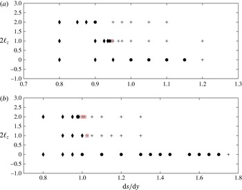
Figure 11. Outcome of the nonlinear interactions between two hetons in the plane
 $(\text{d}s/\text{d}y,\ell _{z})$
, for
$(\text{d}s/\text{d}y,\ell _{z})$
, for
 $\text{d}y/\text{d}z=2$
, and (a)
$\text{d}y/\text{d}z=2$
, and (a)
 ${\it\rho}=0.5$
and (b)
${\it\rho}=0.5$
and (b)
 ${\it\rho}=1$
. Symbols: ♦, recombination as dipoles; ●, formation of a
${\it\rho}=1$
. Symbols: ♦, recombination as dipoles; ●, formation of a
 $Z$
-vortex; and
$Z$
-vortex; and
 $+$
, deviation of the hetons. A red box indicates that a
$+$
, deviation of the hetons. A red box indicates that a
 $Z$
-vortex tends to form but breaks rapidly – indicating the possible presence of metastable
$Z$
-vortex tends to form but breaks rapidly – indicating the possible presence of metastable
 $Z$
-vortex configuration in the vicinity in the parameter space (not reached in practice).
$Z$
-vortex configuration in the vicinity in the parameter space (not reached in practice).
More illustrations of the formation of
 $Z$
-vortices are presented in § A.3. However, they follow the same pattern. The
$Z$
-vortices are presented in § A.3. However, they follow the same pattern. The
 $Z$
-vortex is formed when the horizontal offset between the two incoming hetons
$Z$
-vortex is formed when the horizontal offset between the two incoming hetons
 $\text{d}s$
is slightly less than the corresponding critical separation distance for the existence of the collinear equilibrium. This is required since during the initial phase of the approach this distance tends to increase, which can be justified by the criterion (3.1). Eventually, when in the vicinity of one another, the vortices may combine to form the quadrupole. This formation and the persistence of the quadrupole are related both to the deformation and ability to adapt of the vortices, and to their finite size which distributed the potential vorticity. Note, however, that even spheres, which are nearly equivalent to point vortices, can still form a
$\text{d}s$
is slightly less than the corresponding critical separation distance for the existence of the collinear equilibrium. This is required since during the initial phase of the approach this distance tends to increase, which can be justified by the criterion (3.1). Eventually, when in the vicinity of one another, the vortices may combine to form the quadrupole. This formation and the persistence of the quadrupole are related both to the deformation and ability to adapt of the vortices, and to their finite size which distributed the potential vorticity. Note, however, that even spheres, which are nearly equivalent to point vortices, can still form a
 $Z$
quadrupole due to their ability to deform.
$Z$
quadrupole due to their ability to deform.
5 Finite-core hetons: recombination and deviation
For the sake of completeness, we propose an illustration of the full dynamics for the two generic regimes where the hetons do not form a quadrupole. In the first one, we illustrate the interaction between hetons which recombine as same-depth dipoles. In the second one, the hetons just deviate from their trajectories. Again, these illustrations are generic of all cases in their respective regimes, at least when the initial hetons are stable, and do not break baroclinically before interacting. In the case of breaking hetons, a fraction of the initial hetons may still interact in a similar way, or the resulting secondary vortices may reconfigure in such a way that there are no longer pairs of hetons moving towards one another. Illustrations of unstable interacting hetons were considered in Reinaud & Carton (Reference Reinaud and Carton2015a
) for
 $\text{d}s=0$
and are not further illustrated for small
$\text{d}s=0$
and are not further illustrated for small
 $\text{d}s$
in the present paper. For very large
$\text{d}s$
in the present paper. For very large
 $\text{d}s$
, hetons behave in a similar way to isolated hetons (albeit a small deflection) and their dynamics would be similar to those of isolated hetons, whose stability properties are known (see Reinaud Reference Reinaud2015).
$\text{d}s$
, hetons behave in a similar way to isolated hetons (albeit a small deflection) and their dynamics would be similar to those of isolated hetons, whose stability properties are known (see Reinaud Reference Reinaud2015).
The first case illustrates the recombination of the vortices as same-depth dipoles. Again, we set
 $\text{d}y/\text{d}z=2$
and
$\text{d}y/\text{d}z=2$
and
 $\ell _{z}=0$
, with
$\ell _{z}=0$
, with
 ${\it\rho}=0.5$
. This corresponds again to
${\it\rho}=0.5$
. This corresponds again to
 $d_{y}=\text{d}y/r=4$
. We know that the recombination occurs for small
$d_{y}=\text{d}y/r=4$
. We know that the recombination occurs for small
 $\text{d}s$
, hence we take
$\text{d}s$
, hence we take
 $\text{d}s/\text{d}y=0.5$
. Results are presented in figure 12. This is qualitatively similar to cases with
$\text{d}s/\text{d}y=0.5$
. Results are presented in figure 12. This is qualitatively similar to cases with
 $\text{d}s=0$
, apart from the angle at which the dipoles escape. Such cases are detailed in Reinaud & Carton (Reference Reinaud and Carton2015a
). Again, it should be noted that these cases are generic of small
$\text{d}s=0$
, apart from the angle at which the dipoles escape. Such cases are detailed in Reinaud & Carton (Reference Reinaud and Carton2015a
). Again, it should be noted that these cases are generic of small
 $\text{d}s$
but for cases where the hetons are unstable prior to the interaction.
$\text{d}s$
but for cases where the hetons are unstable prior to the interaction.

Figure 12. PV for the nonlinear evolution for two interacting hetons with
 ${\it\rho}=0.5$
,
${\it\rho}=0.5$
,
 $\ell _{z}=0$
,
$\ell _{z}=0$
,
 $d_{y}=4$
and
$d_{y}=4$
and
 $d_{s}=0.5$
such that the point equivalent is
$d_{s}=0.5$
such that the point equivalent is
 $\text{d}z=1$
,
$\text{d}z=1$
,
 $\text{d}y=2$
and
$\text{d}y=2$
and
 $\text{d}s=2$
. Times displayed are
$\text{d}s=2$
. Times displayed are
 $t=0$
(a), 25 (b), 50 (c) and 75 (d). The hetons are viewed orthographically at an angle of
$t=0$
(a), 25 (b), 50 (c) and 75 (d). The hetons are viewed orthographically at an angle of
 $60^{\circ }$
from the vertical.
$60^{\circ }$
from the vertical.
The next case illustrates the final regime where the hetons are horizontally offset not enough to strongly interact but enough to deflect their trajectory as a consequence of the close encounter. This is typically true for offsets large enough compared with the distance between point vortices in the corresponding equilibrium. Results are presented in figure 13 for one case, but they are generic of all such cases for large horizontal offsets.

Figure 13. PV for the nonlinear evolution for two interacting hetons with
 ${\it\rho}=0.5$
,
${\it\rho}=0.5$
,
 $\ell _{z}=0$
,
$\ell _{z}=0$
,
 $d_{y}=4$
and
$d_{y}=4$
and
 $d_{s}=2$
such that the point equivalent is
$d_{s}=2$
such that the point equivalent is
 $\text{d}z=1$
,
$\text{d}z=1$
,
 $\text{d}y=2$
and
$\text{d}y=2$
and
 $\text{d}s=2$
. Times displayed are
$\text{d}s=2$
. Times displayed are
 $t=0$
(a), 25 (b), 50 (c) and 57 (d). The hetons are viewed orthographically at an angle of
$t=0$
(a), 25 (b), 50 (c) and 57 (d). The hetons are viewed orthographically at an angle of
 $60^{\circ }$
from the vertical.
$60^{\circ }$
from the vertical.
6 Conclusion
This paper has addressed the complex interaction between two hetons which are offset horizontally. We have considered the particular situation when the vortices of the hetons lying at the same depth have opposite polarity, a situation referred to as ‘antisymmetric’ hetons in Reinaud & Carton (Reference Reinaud and Carton2015a
). In this context, we have seen that there are, in general, three main regimes of interaction. The kind of interaction crucially depends on the horizontal offset between the axis along which the individual hetons initially translate. The critical values for which we have the transition from one regime to another are given by a very complex function of all the parameters of the flow, such as the aspect ratio for the hetons’ vortices
 ${\it\rho}=rh$
, the vertical gap between the upper and lower vortices within the hetons
${\it\rho}=rh$
, the vertical gap between the upper and lower vortices within the hetons
 $\ell _{z}$
, and the horizontal offset between the vortices of the hetons
$\ell _{z}$
, and the horizontal offset between the vortices of the hetons
 $d_{y}$
. There are, however, simple ways to estimate a range for the values of the critical offsets separating the different regimes. These ranges can be determined in fact from a simple point vortex calculation. The rationale behind this is as follows. We know that, for antisymmetric hetons, the two incoming baroclinic structures recombine as same-depth dipoles which escape at a right angle when the offset between the two hetons is zero (head-on collision); see for example Reinaud & Carton (Reference Reinaud and Carton2015a
). As a consequence, hetons which are only slightly offset will exhibit a similar behaviour and will separate, recombining as dipoles which escape at an angle depending on the offset.
$d_{y}$
. There are, however, simple ways to estimate a range for the values of the critical offsets separating the different regimes. These ranges can be determined in fact from a simple point vortex calculation. The rationale behind this is as follows. We know that, for antisymmetric hetons, the two incoming baroclinic structures recombine as same-depth dipoles which escape at a right angle when the offset between the two hetons is zero (head-on collision); see for example Reinaud & Carton (Reference Reinaud and Carton2015a
). As a consequence, hetons which are only slightly offset will exhibit a similar behaviour and will separate, recombining as dipoles which escape at an angle depending on the offset.
For large offsets, the interaction between the hetons becomes weak. Indeed, in all our cases, the net strength of each heton is zero, hence their distant influence is very weak indeed. As a consequence, the hetons will only deviate in their trajectory. The deviation becomes smaller as the offset is increased.
These two different behaviours compete in an intermediate range for the horizontal offsets between the incoming hetons. There, the incoming hetons may start to rotate around one another, creating a compound quadrupolar structure. Owing to its apparent shape, the structure is referred to as a
 $Z$
-vortex. The formation of such a structure is triggered by the existence of an exact equilibrium for a set of four point vortices. In these equilibria, the four point vortices are aligned horizontally (albeit they do not all lie at the same depth) and they rotate uniformly with respect to a vertical axis (which coincides with an axis of horizontal symmetry for the configuration). The exact relative position of the vortices can be obtained, and provides an indication of the conditions of formation of the
$Z$
-vortex. The formation of such a structure is triggered by the existence of an exact equilibrium for a set of four point vortices. In these equilibria, the four point vortices are aligned horizontally (albeit they do not all lie at the same depth) and they rotate uniformly with respect to a vertical axis (which coincides with an axis of horizontal symmetry for the configuration). The exact relative position of the vortices can be obtained, and provides an indication of the conditions of formation of the
 $Z$
-vortex. For point vortices, the configuration cannot be reached from two incoming singular hetons from afar. This is naturally due to the fact that the point vortices need to lie on the circular trajectories at all times to be in equilibrium (they cannot reach an equilibrium configuration from a non-equilibrium situation without external action). However, it has been shown that finite-volume vortices are capable of forming
$Z$
-vortex. For point vortices, the configuration cannot be reached from two incoming singular hetons from afar. This is naturally due to the fact that the point vortices need to lie on the circular trajectories at all times to be in equilibrium (they cannot reach an equilibrium configuration from a non-equilibrium situation without external action). However, it has been shown that finite-volume vortices are capable of forming
 $Z$
-vortices due to their ability to deform and adapt to the then time-dependent straining field the vortices induce on one another. It has been shown that flatter vortices are more capable of adapting, arguably due to the larger horizontal overlap for vortices offset in the vertical. The vertical separation between the vortices of the hetons acts as a deterrent for the formation of the
$Z$
-vortices due to their ability to deform and adapt to the then time-dependent straining field the vortices induce on one another. It has been shown that flatter vortices are more capable of adapting, arguably due to the larger horizontal overlap for vortices offset in the vertical. The vertical separation between the vortices of the hetons acts as a deterrent for the formation of the
 $Z$
-vortex while not preventing it (examples of
$Z$
-vortex while not preventing it (examples of
 $Z$
-vortices for offset vortices may be found). The present paper has focused on a limited selection of cases, due to the very large size of the overall parameter space (whose comprehensive investigation is out of reach). The cases presented are in fact generic of the interaction over a large range of parameters. To complement this, the summary outcome of a larger number of cases run over the course of this study is available in § A.3. Further illustrations of the interactions are also available in § A.3.
$Z$
-vortices for offset vortices may be found). The present paper has focused on a limited selection of cases, due to the very large size of the overall parameter space (whose comprehensive investigation is out of reach). The cases presented are in fact generic of the interaction over a large range of parameters. To complement this, the summary outcome of a larger number of cases run over the course of this study is available in § A.3. Further illustrations of the interactions are also available in § A.3.
This paper has addressed a complex problem over a wide parameter space, even after having restricted our interest to some idealised situations in which the hetons are similar (all the vortices have same volume and the same potential vorticity in absolute value).
There is a natural extension of the problem to more practical issues in the oceans. One may be interested in studying the interaction between hetons associated with higher Rossby numbers, which may be relevant to smaller-scale (sub-mesoscale) structures. This could be done using the closely related numerical method known as the non-hydrostatic contour semi-Lagrangian method, developed by Dritschel & Vìudez (see Vìudez & Dritschel Reference Vìudez and Dritschel2002; Dritschel & Vìudez Reference Dritschel and Vìudez2003).
Appendix A
A.1 Velocities in a regular quadrupole
This is a crude approach in an attempt to separate the two regimes (deflect as hetons or recombine as dipoles). The intermediate regime, when effects compete, is when
 $Z$
-vortices can form. The idea is to focus on the velocity
$Z$
-vortices can form. The idea is to focus on the velocity
 $v$
of one vortex in the inside corner (here vortex 1) and try to see if it will go towards or away from the outside corner, the same depth of the second heton (here vortex 4). Of course, this does not consider relative displacement at this stage, nor the fact that all distances are time-dependent. For the sake of simplicity, the strength of the point vortices is implicitly scaled by
$v$
of one vortex in the inside corner (here vortex 1) and try to see if it will go towards or away from the outside corner, the same depth of the second heton (here vortex 4). Of course, this does not consider relative displacement at this stage, nor the fact that all distances are time-dependent. For the sake of simplicity, the strength of the point vortices is implicitly scaled by
 $4{\rm\pi}$
to avoid rewriting the factor
$4{\rm\pi}$
to avoid rewriting the factor
 $1/4{\rm\pi}$
arising from the Green’s function.
$1/4{\rm\pi}$
arising from the Green’s function.
A.1.1 Velocity
$v$
of point 1

This is given by
 $$\begin{eqnarray}v_{1}={\it\kappa}_{3}\frac{(-\text{d}x)}{(r_{1,3})^{3}}+{\it\kappa}_{4}\frac{(-\text{d}x)}{(r_{1,4})^{3}},\end{eqnarray}$$
where
 $r_{i,j}$
is the distance between vortices
$r_{i,j}$
is the distance between vortices
 $i$
and
$i$
and
 $j$
; thus
$j$
; thus
 $$\begin{eqnarray}v_{1}=-\text{d}x\left(\frac{1}{(\text{d}x^{2}+(\text{d}s-\text{d}y)^{2}+\text{d}z^{2})^{3/2}}-\frac{1}{(\text{d}x^{2}+\text{d}s^{2})^{3/2}}\right).\end{eqnarray}$$
The sign of
 $v_{1}$
is that of
$v_{1}$
is that of
 $$\begin{eqnarray}-\!(\text{d}x^{2}+\text{d}s^{2})^{3/2}+(\text{d}x^{2}+(\text{d}s-\text{d}y)^{2}+\text{d}z^{2})^{3/2},\end{eqnarray}$$
which depends only on (to be positive)
 $$\begin{eqnarray}\text{d}x^{2}+\text{d}s^{2}<\text{d}x^{2}+(\text{d}s-\text{d}y)^{2}+\text{d}z^{2},\end{eqnarray}$$
that is
 $$\begin{eqnarray}\displaystyle & \text{d}s^{2}<\text{d}s^{2}-2\,\text{d}s\,\text{d}y+\text{d}y^{2}+\text{d}z^{2}, & \displaystyle\end{eqnarray}$$
 $$\begin{eqnarray}\displaystyle & 2\,\text{d}s\,\text{d}y<\text{d}y^{2}+\text{d}z^{2}. & \displaystyle\end{eqnarray}$$
Thus
 $$\begin{eqnarray}\frac{\text{d}s}{\text{d}y}<\frac{1+(\text{d}z/\text{d}y)^{2}}{2}.\end{eqnarray}$$
For
 $\text{d}s/\text{d}y\ll (1+(\text{d}z/\text{d}y)^{2})/2$
,
$\text{d}s/\text{d}y\ll (1+(\text{d}z/\text{d}y)^{2})/2$
,
 $v_{1}>0$
, and one expects an escape as dipoles, as vortex 1 tends to move towards vortex 4 (which will be the second vortex in the pair). Recall that, for
$v_{1}>0$
, and one expects an escape as dipoles, as vortex 1 tends to move towards vortex 4 (which will be the second vortex in the pair). Recall that, for
 $\text{d}s=0$
,
$\text{d}s=0$
,
 $v_{1}$
is always negative. For
$v_{1}$
is always negative. For
 $\text{d}s/\text{d}y\gg (1+(\text{d}z/\text{d}y)^{2})/2$
,
$\text{d}s/\text{d}y\gg (1+(\text{d}z/\text{d}y)^{2})/2$
,
 $v_{1}<0$
, the heton is deflected to the right. For
$v_{1}<0$
, the heton is deflected to the right. For
 $\text{d}s/\text{d}y\sim (1+(\text{d}z/\text{d}y)^{2})/2$
, effects compete in a complex time-dependent way.
$\text{d}s/\text{d}y\sim (1+(\text{d}z/\text{d}y)^{2})/2$
, effects compete in a complex time-dependent way.
A.1.2 Velocity
$u$
of point 1

This is given by
 $$\begin{eqnarray}\displaystyle & \displaystyle u_{1}\propto -{\it\kappa}_{2}\frac{\text{d}y}{(r_{1,2})^{3}}-{\it\kappa}_{3}\frac{\text{d}y-\text{d}s}{(r_{1,3})^{3}}-{\it\kappa}_{4}\frac{(-\text{d}s)}{(r_{1,4})^{3}}, & \displaystyle\end{eqnarray}$$
 $$\begin{eqnarray}\displaystyle & \displaystyle u_{1}\propto \frac{\text{d}y}{(\text{d}y^{2}+\text{d}z^{2})^{3/2}}-\frac{\text{d}y-\text{d}s}{(\text{d}x^{2}+(\text{d}y-\text{d}s)^{2}+\text{d}z^{2})^{3/2}}+\frac{-\text{d}s}{(\text{d}x^{2}+\text{d}s^{2})^{3/2}}, & \displaystyle\end{eqnarray}$$
 $$\begin{eqnarray}\displaystyle u_{1} & \propto & \displaystyle \text{d}y\left[\frac{1}{(\text{d}y^{2}+\text{d}z^{2})^{3/2}}-\frac{1}{(\text{d}x^{2}+(\text{d}y-\text{d}s)^{2}+\text{d}z^{2})^{3/2}}\right]\nonumber\\ \displaystyle & & \displaystyle +\,\text{d}s\left[\frac{1}{(\text{d}x^{2}+(\text{d}s-\text{d}y)^{2}+\text{d}z^{2})^{3/2}}-\frac{1}{(\text{d}x^{2}+\text{d}s^{2})^{3/2}}\right].\end{eqnarray}$$
We have the following three limiting cases.
-
(i)
$\text{d}s=0$
(known), for which (A 11)This is always positive (the hetons go towards each other). The velocity goes to
$$\begin{eqnarray}u_{1}\propto \text{d}y\left[\frac{1}{(\text{d}y^{2}+\text{d}z^{2})^{3/2}}-\frac{1}{(\text{d}x^{2}+(\text{d}y-\text{d}s)^{2}+\text{d}z^{2})^{3/2}}\right].\end{eqnarray}$$
$0$
as
${\rm\Delta}x$
goes to 0, i.e. as the hetons get closer.
-
(ii)
$\text{d}y$
very small, for which (A 12)Again, this is 0 when
$$\begin{eqnarray}u_{1}\sim \text{d}s\left[\frac{1}{(\text{d}x^{2}+\text{d}s^{2}+\text{d}z^{2})^{3/2}}-\frac{1}{(\text{d}x^{2}+\text{d}s^{2})^{3/2}}\right].\end{eqnarray}$$
$\text{d}x\rightarrow 0$
. Otherwise this would be negative and would be the dominant term corresponding to the negative (clockwise) rotation of vortices 1 and 4. This regime is not of interest in this study.
-
(iii)
$\text{d}s=\text{d}y$
, for which (A 13)Initially, for large
$$\begin{eqnarray}u_{1}\propto \text{d}y\left[\frac{1}{(\text{d}y^{2}+\text{d}z^{2})^{3/2}}-\frac{1}{(\text{d}y^{2}+\text{d}x^{2})^{3/2}}\right].\end{eqnarray}$$
$\text{d}x$
,
$u_{1}$
is positive and decreases as
$\text{d}x$
decreases to
$\text{d}z$
.


A.2
$Z$
-vortex equilibria for point vortices

Consider two collinear hetons, as shown in the geometry in figure 14. The four singularities are aligned in the
 $y{-}z$
plane. We write down the velocity
$y{-}z$
plane. We write down the velocity
 $u$
, perpendicular to this plane, for the singularity, assuming that we are placed in a uniform rotation
$u$
, perpendicular to this plane, for the singularity, assuming that we are placed in a uniform rotation
 ${\it\Omega}$
about the
${\it\Omega}$
about the
 $z$
-axis. We are looking for solutions where we can find
$z$
-axis. We are looking for solutions where we can find
 $u=0$
for all singularities, i.e. the flow is steady. By construction
$u=0$
for all singularities, i.e. the flow is steady. By construction
 $v=0$
. By symmetry, it is easy to show that
$v=0$
. By symmetry, it is easy to show that
 $u_{3}=-u_{1}$
and
$u_{3}=-u_{1}$
and
 $u_{2}=-u_{4}$
. Therefore we only need to focus on
$u_{2}=-u_{4}$
. Therefore we only need to focus on
 $u_{1}=0$
and
$u_{1}=0$
and
 $u_{2}=0$
. Each of these equations will give a condition on
$u_{2}=0$
. Each of these equations will give a condition on
 ${\it\Omega}$
which will depend on both parameters
${\it\Omega}$
which will depend on both parameters
 $\text{d}y/\text{d}z$
and
$\text{d}y/\text{d}z$
and
 $\text{d}s/\text{d}z$
. For the equilibrium to exist, the condition needs to be unique, hence imposing a constraint
$\text{d}s/\text{d}z$
. For the equilibrium to exist, the condition needs to be unique, hence imposing a constraint
 $f(\text{d}y/\text{d}z,\text{d}s\cdot \text{d}z)=0$
. The geometry and the parameters are defined in figure 14.
$f(\text{d}y/\text{d}z,\text{d}s\cdot \text{d}z)=0$
. The geometry and the parameters are defined in figure 14.

Figure 14. Description of the geometry for the collinear
 $Z$
-vortex. The black discs indicate the two positive vortices.
$Z$
-vortex. The black discs indicate the two positive vortices.
The equations read
 $$\begin{eqnarray}\displaystyle & \displaystyle u_{1}=-{\it\kappa}_{2}\frac{(y_{1}-y_{2})}{(r_{1,2})^{3}}-{\it\kappa}_{3}\frac{(y_{1}-y_{3})}{(r_{1,3})^{3}}-{\it\kappa}_{4}\frac{(y_{1}-y_{4})}{(r_{1,4})^{3}}+{\it\Omega}y_{1}, & \displaystyle\end{eqnarray}$$
 $$\begin{eqnarray}\displaystyle & \displaystyle u_{2}=-{\it\kappa}_{1}\frac{(y_{2}-y_{1})}{(r_{1,2})^{3}}-{\it\kappa}_{3}\frac{(y_{2}-y_{3})}{(r_{2,3})^{3}}-{\it\kappa}_{4}\frac{(y_{2}-y_{4})}{(r_{2,4})^{3}}+{\it\Omega}y_{2}, & \displaystyle\end{eqnarray}$$
 $$\begin{eqnarray}\displaystyle & \displaystyle u_{1}=-\frac{\text{d}y}{(\text{d}y^{2}+\text{d}z^{2})^{3/2}}-\frac{(\text{d}s-\text{d}y)}{((\text{d}s-\text{d}y)^{2}+\text{d}z^{2})^{3/2}}+\frac{1}{\text{d}s^{2}}+{\it\Omega}\frac{\text{d}s-\text{d}y}{2}, & \displaystyle\end{eqnarray}$$
 $$\begin{eqnarray}\displaystyle & \displaystyle u_{2}=-\frac{(\text{d}y)}{(\text{d}y^{2}+\text{d}z^{2})^{3/2}}-\frac{1}{\text{d}s^{2}}+\frac{(\text{d}s+\text{d}y)}{((\text{d}s+\text{d}y)^{2}+\text{d}z^{2})^{3/2}}+{\it\Omega}\frac{\text{d}s+\text{d}y}{2}=0. & \displaystyle\end{eqnarray}$$
Adding the two equations and subtracting them gives
 $$\begin{eqnarray}\displaystyle & \displaystyle {\it\Omega}\text{d}s-2\frac{\text{d}y}{(\text{d}y^{2}+\text{d}z^{2})^{3/2}}-\frac{(\text{d}s-\text{d}y)}{((\text{d}s-\text{d}y)^{2}+\text{d}z^{2})^{3/2}}+\frac{(\text{d}s+\text{d}y)}{((\text{d}s+\text{d}y)^{2}+\text{d}z^{2})^{3/2}}=0,\qquad & \displaystyle\end{eqnarray}$$
 $$\begin{eqnarray}\displaystyle & \displaystyle {\it\Omega}\text{d}y+\frac{(\text{d}s+\text{d}y)}{((\text{d}s+\text{d}y)^{2}+\text{d}z^{2})^{3/2}}+\frac{(\text{d}s-\text{d}y)}{((\text{d}s-\text{d}y)^{2}+\text{d}z^{2})^{3/2}}-\frac{2}{\text{d}s^{2}}=0. & \displaystyle\end{eqnarray}$$
Multiplying the former equation by
 $\text{d}y$
and subtracting the latter multiplied by
$\text{d}y$
and subtracting the latter multiplied by
 $\text{d}s$
allows us to eliminate
$\text{d}s$
allows us to eliminate
 ${\it\Omega}$
and we finally obtain
${\it\Omega}$
and we finally obtain
 $$\begin{eqnarray}\displaystyle & & \displaystyle \left(\left(\frac{\text{d}s}{\text{d}z}\right)^{2}-\left(\frac{\text{d}y}{\text{d}z}\right)^{2}\right)\left(\frac{1}{\left(1+\left(\displaystyle \frac{\text{d}y-\text{d}s}{\text{d}z}\right)^{2}\right)^{3/2}}+\frac{1}{\left(1+\left(\displaystyle \frac{\text{d}y+\text{d}s}{\text{d}z}\right)^{2}\right)^{3/2}}\right)\nonumber\\ \displaystyle & & \displaystyle \quad \qquad =2\left(\frac{1}{(\text{d}s/\text{d}z)}-\frac{(\text{d}y/\text{d}z)^{2}}{(1+(\text{d}y/\text{d}z)^{2})^{3/2}}\right)\end{eqnarray}$$
after term cancellations.

Figure 15. Growth rate
 ${\it\sigma}_{r}$
of the most unstable mode (red) versus
${\it\sigma}_{r}$
of the most unstable mode (red) versus
 $\text{d}y$
at equilibrium for
$\text{d}y$
at equilibrium for
 $\text{d}z=1$
(the corresponding value of
$\text{d}z=1$
(the corresponding value of
 $\text{d}s$
can be obtained from figure 3), and frequencies
$\text{d}s$
can be obtained from figure 3), and frequencies
 ${\it\sigma}_{i}$
(black) of neutrally stable modes.
${\it\sigma}_{i}$
(black) of neutrally stable modes.
Linearising the full equations of motion of the four singularities about the equilibrium (in the reference frame rotating with the equilibrium), we study the linear stability of infinitesimal perturbations
 $(x_{i}^{\prime },y_{i}^{\prime })$
,
$(x_{i}^{\prime },y_{i}^{\prime })$
,
 $i=1,2,3,4$
. This provides eight eigenmodes
$i=1,2,3,4$
. This provides eight eigenmodes
 ${\it\sigma}={\it\sigma}_{r}+\text{i}{\it\sigma}_{r}$
(one for each perturbed variable) where the time dependence of the perturbation is proportional to
${\it\sigma}={\it\sigma}_{r}+\text{i}{\it\sigma}_{r}$
(one for each perturbed variable) where the time dependence of the perturbation is proportional to
 $\text{e}^{{\it\sigma}t}$
. The real part
$\text{e}^{{\it\sigma}t}$
. The real part
 ${\it\sigma}_{r}$
of
${\it\sigma}_{r}$
of
 ${\it\sigma}$
is the growth rate of the perturbation, while its imaginary part is a frequency. Results are shown in figure 15.
${\it\sigma}$
is the growth rate of the perturbation, while its imaginary part is a frequency. Results are shown in figure 15.

Figure 16. Trajectories of the unstable point vortex quadrupole equilibria for
 $\text{d}y=0.7$
.
$\text{d}y=0.7$
.
It is shown that there is an unstable mode vanishing at
 $\text{d}y\sim 0$
, and at
$\text{d}y\sim 0$
, and at
 $\text{d}y\simeq 0.895$
. At
$\text{d}y\simeq 0.895$
. At
 $\text{d}y\simeq 0.895$
, we find a classical pattern of exchange of instability where a mode
$\text{d}y\simeq 0.895$
, we find a classical pattern of exchange of instability where a mode
 ${\it\sigma}=\text{i}{\it\sigma}_{i}$
with a non-zero frequency decreases rapidly as
${\it\sigma}=\text{i}{\it\sigma}_{i}$
with a non-zero frequency decreases rapidly as
 $\text{d}y$
is decreased. It eventually collapses to zero and the mode becomes unstable. It should be noted that in fact all modes go in pairs. That is, if
$\text{d}y$
is decreased. It eventually collapses to zero and the mode becomes unstable. It should be noted that in fact all modes go in pairs. That is, if
 ${\it\sigma}$
is an eigenvalue, so is
${\it\sigma}$
is an eigenvalue, so is
 $-{\it\sigma}$
. This means that to all unstable modes
$-{\it\sigma}$
. This means that to all unstable modes
 ${\it\sigma}_{r}>0$
, there is an associated stable mode
${\it\sigma}_{r}>0$
, there is an associated stable mode
 ${\it\sigma}_{r}<0$
. The negative values of the modes are not represented in figure 15. The example for
${\it\sigma}_{r}<0$
. The negative values of the modes are not represented in figure 15. The example for
 $\text{d}y=1$
presented in figure 16 is indeed linearly stable. An example of the trajectories for an unstable case with
$\text{d}y=1$
presented in figure 16 is indeed linearly stable. An example of the trajectories for an unstable case with
 $\text{d}y=0.7$
is illustrated below. For clarity, the trajectories are given in the reference frame rotating at the rotation rate of the equilibrium (if the state was stable, the trajectories would just be four motionless points).
$\text{d}y=0.7$
is illustrated below. For clarity, the trajectories are given in the reference frame rotating at the rotation rate of the equilibrium (if the state was stable, the trajectories would just be four motionless points).
A.3 Outcome of the full nonlinear simulations
Here we propose tables summarising the outcome of a large series of numerical experiments realised during this research.
We next provide some complementary material to the results presented in the main part of the paper.
Table 1. Summary of the behaviour of a pair of interacting antisymmetric hetons.

A.4 First case, wide vortices:
${\it\rho}=3.5$
,
$\ell _{z}=1.5$
,
$d_{y}=2$
and
$d_{s}=1$


Table 1 in § A.3 indicates that the case with
 ${\it\rho}=3.5$
,
${\it\rho}=3.5$
,
 $\ell _{z}=1.5$
,
$\ell _{z}=1.5$
,
 $d_{y}=2$
and
$d_{y}=2$
and
 $d_{s}=1$
exhibits the formation of a
$d_{s}=1$
exhibits the formation of a
 $Z$
-vortex in the full quasi-geostrophic numerical simulation using contour surgery. This case has parameters rather different from the ones illustrated in the main paper and therefore are worth showing. Indeed, here the vortices are much flatter than in the illustrative case shown in the paper (
$Z$
-vortex in the full quasi-geostrophic numerical simulation using contour surgery. This case has parameters rather different from the ones illustrated in the main paper and therefore are worth showing. Indeed, here the vortices are much flatter than in the illustrative case shown in the paper (
 ${\it\rho}=3.5$
instead of 0.5 or 2). This allowed us to find a
${\it\rho}=3.5$
instead of 0.5 or 2). This allowed us to find a
 $Z$
-vortex for a moderate vertical offset. This illustrates further that the formation of a
$Z$
-vortex for a moderate vertical offset. This illustrates further that the formation of a
 $Z$
-vortex, albeit being made more difficult for increasing vertical separation, is not prohibited by it.
$Z$
-vortex, albeit being made more difficult for increasing vertical separation, is not prohibited by it.

Figure 17. Trajectories of the centres of the vortices (four largest vortices in the contour surgery case) for
 ${\it\rho}=3.5$
,
${\it\rho}=3.5$
,
 $\ell _{z}=1.5$
,
$\ell _{z}=1.5$
,
 $d_{y}=2$
and
$d_{y}=2$
and
 $d_{s}=1$
. Point vortices (a), ellipsoidal model (b), and contour surgery (c).
$d_{s}=1$
. Point vortices (a), ellipsoidal model (b), and contour surgery (c).

Figure 18. Case 1 (
 ${\it\rho}=3.5,\ell _{z}=1.5$
,
${\it\rho}=3.5,\ell _{z}=1.5$
,
 $d_{y}=2$
and
$d_{y}=2$
and
 $d_{s}=1$
): snapshots of the evolution of the hetons from the full quasi-geostrophic dynamics with contour dynamics at time
$d_{s}=1$
): snapshots of the evolution of the hetons from the full quasi-geostrophic dynamics with contour dynamics at time
 $t=0$
(a), 50 (b), 60 (c) and 172 (d).
$t=0$
(a), 50 (b), 60 (c) and 172 (d).

Figure 19. Case 1 (
 ${\it\rho}=3.5,\ell _{z}=1.5$
,
${\it\rho}=3.5,\ell _{z}=1.5$
,
 $d_{y}=2$
and
$d_{y}=2$
and
 $d_{s}=1$
): ellipsoidal model equivalent.
$d_{s}=1$
): ellipsoidal model equivalent.

Figure 20. Case 1: point vortex. Examination of trajectories near the formation of the
 $Z$
-vortex case 1,
$Z$
-vortex case 1,
 $\text{d}y/\text{d}z=2.8$
,
$\text{d}y/\text{d}z=2.8$
,
 $\text{d}s/\text{d}y=12.9/14$
(a),
$\text{d}s/\text{d}y=12.9/14$
(a),
 $12.94/14$
(b),
$12.94/14$
(b),
 $12.95/14$
(c),
$12.95/14$
(c),
 $12.96/14$
(d),
$12.96/14$
(d),
 $13/14$
(e), and
$13/14$
(e), and
 $13.4/14$
(f).
$13.4/14$
(f).
The set-up means that the centre separation of the vortices is as follows:
 $\text{d}y/\text{d}z=2.8$
. The equivalent point vortex collinear equilibria would correspond to
$\text{d}y/\text{d}z=2.8$
. The equivalent point vortex collinear equilibria would correspond to
 $\text{d}s/\text{d}z=2.82$
(i.e.
$\text{d}s/\text{d}z=2.82$
(i.e.
 $\text{d}s/\text{d}y=0.993\simeq 1$
).
$\text{d}s/\text{d}y=0.993\simeq 1$
).
We first illustrate the trajectory of the vortex centres, comparing again the three models available to us, namely point vortex dynamics, the ellipsoidal vortex model and the full quasi-geostrophic dynamics (with contour dynamics). Results are presented in figure 17.
The full quasi-geostrophic evolution is illustrated for this case in figure 18. Its equivalent using the simplified ellipsoidal model is given in figure 19. Both show the formation of the
 $Z$
quadrupole.
$Z$
quadrupole.
Again, this shows that the deformation of the vortices stabilised the quasi-periodic trajectory. In figure 20, we examine in more detail the trajectory of singular vortices, to illustrate the extreme sensitivity of the singularities’ trajectories to the set-up.
Going back to the finite-core vortices, and for such a configuration with wide poles, the
 $Z$
-quadrupolar configuration can even be achieved for larger
$Z$
-quadrupolar configuration can even be achieved for larger
 $d_{s}=\text{d}s/\text{d}y$
, as shown in figure 21 with
$d_{s}=\text{d}s/\text{d}y$
, as shown in figure 21 with
 $d_{s}=2$
(instead of 1).
$d_{s}=2$
(instead of 1).
A.5 Second case: large horizontal offset
$d_{y}$
, with
${\it\rho}=0.5$
,
$\ell _{z}=0$
,
$d_{y}=5$
and
$d_{s}=1$


In the second case, we go back to the case of hetons with vortices
 ${\it\rho}=0.5$
illustrated in the main text of the paper (figure 7) but with a slightly higher offset between the poles within the hetons. It is shown that the evolution is qualitatively similar, indicating that the case shown in figure 7 is indeed generic. The results are shown in figure 22.
${\it\rho}=0.5$
illustrated in the main text of the paper (figure 7) but with a slightly higher offset between the poles within the hetons. It is shown that the evolution is qualitatively similar, indicating that the case shown in figure 7 is indeed generic. The results are shown in figure 22.
A.6 Dipole/heton
We next illustrate the case where the
 $Z$
-vortex initially forms, but where the strain induced by the vortices onto one another is large enough to destabilise two of the vortices. These vortices break into two pieces, which recombine to produce two structures with an L shape. Each structure consists of three vortices, and is the combination of a heton (two vortices of opposite sign at different depth) and a dipole (two vortices of opposite sign at the same depth). This may happen when the vortices are wide enough to break baroclinically. Such a situation is illustrated in figure 23. This example shows that the flow evolution also depends on the stability properties of the structures that form as a result of the interactions. The fate of interacting, wide, hetons in the case
$Z$
-vortex initially forms, but where the strain induced by the vortices onto one another is large enough to destabilise two of the vortices. These vortices break into two pieces, which recombine to produce two structures with an L shape. Each structure consists of three vortices, and is the combination of a heton (two vortices of opposite sign at different depth) and a dipole (two vortices of opposite sign at the same depth). This may happen when the vortices are wide enough to break baroclinically. Such a situation is illustrated in figure 23. This example shows that the flow evolution also depends on the stability properties of the structures that form as a result of the interactions. The fate of interacting, wide, hetons in the case
 $d_{s}=0$
(head-on collision) is detailed in Reinaud & Carton (Reference Reinaud and Carton2015a
). This indicates that more complex dynamics may be observed if the structures themselves are sensitive to shear- or strain-induced instabilities. The systematic and detailed investigation of these behaviours (done for
$d_{s}=0$
(head-on collision) is detailed in Reinaud & Carton (Reference Reinaud and Carton2015a
). This indicates that more complex dynamics may be observed if the structures themselves are sensitive to shear- or strain-induced instabilities. The systematic and detailed investigation of these behaviours (done for
 $d_{s}=0$
in Reinaud & Carton (Reference Reinaud and Carton2015a
)) is beyond the scope of the present contribution due to the size of the parameter space with the added degree of freedom
$d_{s}=0$
in Reinaud & Carton (Reference Reinaud and Carton2015a
)) is beyond the scope of the present contribution due to the size of the parameter space with the added degree of freedom
 $d_{s}$
.
$d_{s}$
.

Figure 21. Case similar to case 1 but for a larger horizontal offset
 $d_{s}$
. Here
$d_{s}$
. Here
 ${\it\rho}=3.5$
,
${\it\rho}=3.5$
,
 $\ell _{z}=1.5$
,
$\ell _{z}=1.5$
,
 $d_{y}=2$
and
$d_{y}=2$
and
 $d_{s}=2$
. Snapshots displayed at
$d_{s}=2$
. Snapshots displayed at
 $t=7$
(a), 32 (b), 52 (c) and 63 (d).
$t=7$
(a), 32 (b), 52 (c) and 63 (d).

Figure 22. Case 2: contour surgery with
 ${\it\rho}=0.5$
,
${\it\rho}=0.5$
,
 $\ell _{z}=0$
,
$\ell _{z}=0$
,
 $d_{y}=5$
and
$d_{y}=5$
and
 $d_{s}=1$
.
$d_{s}=1$
.

Figure 23. Dipole/heton:
 ${\it\rho}=0.5$
,
${\it\rho}=0.5$
,
 $\ell _{z}=1.5$
,
$\ell _{z}=1.5$
,
 $d_{y}=1.5$
and
$d_{y}=1.5$
and
 $d_{s}=1$
. Times displayed are
$d_{s}=1$
. Times displayed are
 $t=25$
(a), 40 (b), 55 (c) and 65 (d).
$t=25$
(a), 40 (b), 55 (c) and 65 (d).


