


1. Introduction
Studying the transport of bedload sediment particles ranging from coarse sands to gravels can be a challenge due to complex fluid–particle and particle–particle interactions (Gonzalez et al. Reference Gonzalez, Richter, Bolster, Bateman, Calantoni and Escauriaza2017). Depending on the temporal–spatial scale focused on, the underlying mechanisms dominating the bedload transport process can be very different. The pioneering work of Einstein (Reference Einstein1937) considered the transport of bedload particles at a relatively large scale, which involves many entrainment and deposition events experienced by each single particle. He conceptualized this complex transport process as composed of fundamental elements of rests for static particles and hops (or steps) for moving particles. During rests, a particle can stay either on top of the riverbed or buried under the surface. The term ‘hop’ can be formally defined as the successive motions of a particle from the start to the end of its motion, or motions between a pair of adjacent entrainment and deposition events by the same particle. The random variable of hop distance (or step length) with its probability density function (p.d.f.) has since been extensively studied for probabilistic formulations of bedload sediment transport (Paintal Reference Paintal1971; Hassan, Church & Schick Reference Hassan, Church and Schick1991; Parker, Paola & Leclair Reference Parker, Paola and Leclair2000; Ancey et al. Reference Ancey, Davison, Bohm, Jodeau and Frey2008; Ancey Reference Ancey2010; Bradley & Tucker Reference Bradley and Tucker2012; Hassan et al. Reference Hassan, Voepel, Schumer, Parker and Fraccarollo2013; Yager, Kenworthy & Monsalve Reference Yager, Kenworthy and Monsalve2015; Wilson Reference Wilson2018). For example, focusing on the exchange of bedload particles between those in motion and those staying in the riverbed, the streamwise transport of tracer particles has been intensively explored recently, with the aim of understanding the problem of anomalous diffusion. This progress has mostly involved the assumption of a thin-tailed p.d.f. of hop-distances during the implementation of theoretical (Ganti et al. Reference Ganti, Meerschaert, Foufoula-Georgiou, Viparelli and Parker2010; Lajeunesse, Devauchelle & James Reference Lajeunesse, Devauchelle and James2018; Wu et al. Reference Wu, Foufoula-Georgiou, Parker, Singh, Fu and Wang2019a,Reference Wu, Singh, Fu and Wangb), numerical (Fan et al. Reference Fan, Zhong, Wu, Foufoula-Georgiou and Guala2014, Reference Fan, Singh, Guala, Foufoula-Georgiou and Wu2016; Pelosi et al. Reference Pelosi, Schumer, Parker and Ferguson2016) and experimental (Martin, Jerolmack & Schumer Reference Martin, Jerolmack and Schumer2012; Bradley Reference Bradley2017; Liu, Pelosi & Guala Reference Liu, Pelosi and Guala2019) approaches.
At the relatively small scale of bedload particle transport, especially focusing on particle hops, the motions of the entrained particles are complicated and can include rolling, sliding and saltating on top of the riverbed (Charru, Mouilleron & Eiff Reference Charru, Mouilleron and Eiff2004; Lajeunesse, Malverti & Charru Reference Lajeunesse, Malverti and Charru2010; Roseberry, Schmeeckle & Furbish Reference Roseberry, Schmeeckle and Furbish2012; Seizilles et al. Reference Seizilles, Lajeunesse, Devauchelle and Bak2014; Fathel, Furbish & Schmeeckle Reference Fathel, Furbish and Schmeeckle2015; Ballio et al. Reference Ballio, Radice, Fathel and Furbish2019; Hosseini-Sadabadi, Radice & Ballio Reference Hosseini-Sadabadi, Radice and Ballio2019). To better characterize the hop distance as well as other kinematic quantities, detailed information regarding the motions of sediment particles during transport is required, which has led to several high-resolution bedload particle-tracking experiments in the past decade, capturing the trajectories of every moving particle (Charru et al. Reference Charru, Mouilleron and Eiff2004; Lajeunesse et al. Reference Lajeunesse, Malverti and Charru2010; Martin et al. Reference Martin, Jerolmack and Schumer2012; Roseberry et al. Reference Roseberry, Schmeeckle and Furbish2012; Ancey & Heyman Reference Ancey and Heyman2014; Seizilles et al. Reference Seizilles, Lajeunesse, Devauchelle and Bak2014; Campagnol et al. Reference Campagnol, Radice, Ballio and Nikora2015; Liu et al. Reference Liu, Pelosi and Guala2019). The probability distributions for various kinematic quantities were then obtained empirically, including those of velocities, accelerations, hop distances, and travel times (time spent during a hop, denoted as  $\tau$ in this paper). These results are key for understanding the underlying physics of hop processes, as well as assisting in theoretical formulations and numerical simulation, and serving as additional means of validation for the modelling of bedload sediment transport (Ancey & Heyman Reference Ancey and Heyman2014; Fan et al. Reference Fan, Zhong, Wu, Foufoula-Georgiou and Guala2014).
Based on numerical simulations and experimental measurements, Wu, Furbish & Foufoula-Georgiou (Reference Wu, Furbish and Foufoula-Georgiou2020) identified two distinct transport regimes for short and long hops, the mean hop distances ( $L_h$) of which scale with their travel times (
 $\tau$) quadratically (
 $L_h \sim \tau ^2$) and linearly (
 $L_h \sim \tau$), respectively. This observation was critical to unify disparate views on particle velocity statistics (exponential versus Gaussian) reported in the literature, demonstrating that long hops alone contribute to the Gaussian type of particle velocity p.d.f., while a mixture of both short and long hops leads to the exponential distribution, commonly observed at low transport rates. Under the well-accepted assumption of an exponential travel-time distribution (Lajeunesse et al. Reference Lajeunesse, Malverti and Charru2010; Martin et al. Reference Martin, Jerolmack and Schumer2012; Fathel et al. Reference Fathel, Furbish and Schmeeckle2015; Liu et al. Reference Liu, Pelosi and Guala2019), the linear scaling relation for long hops was linked to the empirical evidence of thin-tailed hop-distance distribution. However, since the governing equation can only be solved numerically, no analytical arguments were made to provide a theoretical basis for such scaling regimes in the mean hop distance–travel time relation (
 $L_h$–
 $\tau$) (Wu et al. Reference Wu, Furbish and Foufoula-Georgiou2020). Consequently, a previous formulation of a mean-reverting process (Ancey & Heyman Reference Ancey and Heyman2014) was resorted to in order to understand the motion of the long-hop particles (Wu et al. Reference Wu, Furbish and Foufoula-Georgiou2020). For short hops, however, which may cover over 80 % of the overall hops, there is still the lack of a theory that explains the hop distance–travel time scaling, leading to ambiguity in the scaling exponent reported in the literature (Roseberry et al. Reference Roseberry, Schmeeckle and Furbish2012; Fathel et al. Reference Fathel, Furbish and Schmeeckle2015; Wu et al. Reference Wu, Furbish and Foufoula-Georgiou2020). Given the statistical persistence of short hops, such information is deemed critical for correctly estimating sediment transport rate.
Regarding the governing equation for bedload particle motions adopted by Wu et al. (Reference Wu, Furbish and Foufoula-Georgiou2020), some unknown functions must first be determined before numerical simulations can be performed for particle hops. This is, however, not trivial, and requires high-precision measurements of particle motions enabling the correct estimate of Lagrangian or total acceleration. For example, acceleration estimates from the second derivative of particle positions require an order-of-magnitude higher frequency (250 frames per second) in video capturing (Roseberry et al. Reference Roseberry, Schmeeckle and Furbish2012; Liu et al. Reference Liu, Pelosi and Guala2019), as compared to that in similar studies focusing on particle hop distances and waiting times (Martin et al. Reference Martin, Jerolmack and Schumer2012). Data acquisition on particles’ travel times and hop distances is thus less experimentally demanding: those data are easier to obtain (require much lower sampling frequency), more accurate and more likely to be statistically converged given that measurement duration is typically inversely related to the acquisition frame rate. We expect that a theoretical model that can be parametrized with such data would be more reliable and feasible to apply.
In this paper we mainly aim at theoretically analysing the relation between mean hop distances and travel times ( $L_h$–
 $\tau$ relationship) during bedload particle hops, which provides insights into the shift of scaling regimes as observed by the numerical and experimental investigation of Wu et al. (Reference Wu, Furbish and Foufoula-Georgiou2020). To achieve such a goal, we will characterize the velocity variations during bedload particle hops, embedding the information of accelerations into the derived governing equation. However, we emphasize that we do not attempt a physical interpretation of the velocity variations. The main novelties of the paper are the following. First, we propose a nonlinear transformation of the particle velocity resulting in a velocity difference
  ${\rm \Delta} \zeta$ that can be approximated by a Gaussian random walk process and leads to the governing equation for particle hops (§ 2). Second, we show that the deduced governing equation is intrinsically identical to that describing a Taylor dispersion process for solute transport in shear flows (Taylor Reference Taylor1953; Wu & Chen Reference Wu and Chen2014). Borrowing the analytical technique of concentration moments (Aris Reference Aris1956) employed to study Taylor dispersion, we derive analytical solutions of the p.d.f.s of particles’ travel times and hop distances, and a relation between the mean hop distances and the travel times valid across the whole range of scales involved, both excellently supported by experimental data (Fathel et al. Reference Fathel, Furbish and Schmeeckle2015). We then show that the estimation of the required parameters (e.g. the diffusion coefficient) in the particle motion governing equation can be made based on measurements of hop distances and travel times, with no need for the acceleration data. As a further validation, we confirm that the acceleration distribution obtained from numerical simulations of the proposed particle motion governing equation is consistent with that obtained from experimental measurements (§ 3). Finally, concluding remarks are provided in § 4.
2. Formulation
In this paper we analyse the one-dimensional (streamwise) transport of bedload sediment particles, which are of uniform size and in equilibrium transport conditions. This idealized theoretical set-up is in accordance with recent studies (Lajeunesse et al. Reference Lajeunesse, Malverti and Charru2010; Roseberry et al. Reference Roseberry, Schmeeckle and Furbish2012; Fathel et al. Reference Fathel, Furbish and Schmeeckle2015) on the statistics of particle motions, specifically focusing on events of particle hops. Hops are defined as the successive motions of a sediment particle measured from its start (entrainment) to stop (deposition). The corresponding times spent during the hops are termed as travel times ( $\tau$). For comparison, and validation of our analytical solutions in this study, we used the experimental data presented in Fathel et al. (Reference Fathel, Furbish and Schmeeckle2015), which rely on the experimental measurements of Roseberry et al. (Reference Roseberry, Schmeeckle and Furbish2012). We note that, based on this specific experimental dataset, our approach is relevant for bedload transport under conditions of low transport rates. However, the theoretical findings of this work may have broader implications, e.g. on the scaling relations for particle motions (see also Wu et al. Reference Wu, Furbish and Foufoula-Georgiou2020), which requires further evaluation with different experimental datasets in the future.
2.1. Random walk for particles’ velocity variation  ${\rm \Delta} u$

We are interested in understanding how a bedload particle's velocity can change with time during a hop. In figure 1 we display an example of the velocity trajectory during the hop of a single bedload particle, which is randomly selected from the high-resolution experimental measurements of Fathel et al. (Reference Fathel, Furbish and Schmeeckle2015). At first glance, it is reasonable to speculate that the particle's velocity could be described by a random walk process during the hop:
 \begin{equation} {\rm \Delta} u = u ( {t + {\rm \Delta} t} ) - u (t) = R\sqrt {2{D^*}{\rm \Delta} t}, \end{equation}
where  $u$ is the particle's velocity (m s
 $^{-1}$ ),
  $t$ is time (s),
  ${\rm \Delta} u$ is the change in velocity over an observed time step
  ${\rm \Delta} t$ (in this case an experimental sampling time step as seen in figure 1),
  $D^*$ is a constant diffusion coefficient (m
 $^2$ s
 $^{-3}$ ) and
  $R$ is a random variable with zero mean and unit variance. Note that the requirement of unit variance for
  $R$ here is in accordance with that of a finite second-order moment for the distribution of
  ${\rm \Delta} u$, which guarantees that the random walk process (2.1) will asymptotically approach a diffusion process.

Figure 1. An example of velocity trajectory during the hop of a single bedload particle, which is randomly selected from the high-resolution experimental measurements (Fathel et al. Reference Fathel, Furbish and Schmeeckle2015).
It is easy to check, by putting together all the records of velocity variations  ${\rm \Delta} u$ obtained by taking the difference between successive particle velocities for the observed trajectories, that these fluctuations have zero mean. In addition, the p.d.f.s of
  ${\rm \Delta} u$ based on different sample sizes can be approximated by a stationary distribution, which ensures the unit variance for
  $R$ and a constant diffusion coefficient
  $D^*$ (not shown here).
In the case when the random variable  $R$ follows a Gaussian distribution (on top of zero mean and unit variance as stated above), (2.1) would describe a Gaussian random walk process. This would be particularly interesting because one could immediately infer the form of the governing equation for the particle's velocity variations, since the Gaussian random walk is equivalent to a diffusion equation (e.g. see Li et al. Reference Li, Aubeneau, Bolster, Tank and Packman2017). Accordingly, (2.1) leads to
 \begin{equation} \frac{{\partial {P_N} ( {u,t} )}}{{\partial t}} = {D^*}\frac{{{\partial ^2}{P_N}}}{{\partial {u^2}}}, \end{equation}
where  $P_N$ is the p.d.f. of the particle's velocity under the above assumptions. Note that the form of the distribution for the random variable
  $R$ can be obtained from the acceleration data, which is calculated from
  ${\rm \Delta} u/{\rm \Delta} t$ (which gives the left-hand side of (2.1) and thus specifies the distribution of
  $R$ on the right-hand side of (2.1)).
However, experimental results have already rejected the hypothesis of a Gaussian p.d.f. for  $R$, by showing that the acceleration p.d.f. of particle motions is Laplace-like or double-exponential-like (Fathel et al. Reference Fathel, Furbish and Schmeeckle2015; Liu et al. Reference Liu, Pelosi and Guala2019). In figure 2, we provide the calculated statistics of particle velocity variations for the experimentally measured hops. It is obvious from figure 2(a) that the p.d.f. of the velocity variations can be well approximated by a Laplace distribution. Figure 2(b) presents a quantile–quantile (QQ) plot to quantify how the distribution of
  ${\rm \Delta} u$ deviates from a normal distribution. Notice that in figure 2 we have scaled the velocity variation
  ${\rm \Delta} u$ by a characteristic maximum velocity
  $u_0 = U_{max}$. We now infer that the velocity variations of bedload particle hops measured along the
  $u$-axis may possibly follow a random walk, but not a Gaussian random walk process.

Figure 2. Bedload particle velocity variation statistics for the experimentally measured hops (Fathel et al. Reference Fathel, Furbish and Schmeeckle2015). (a) The p.d.f. of the experimentally measured velocity variations. Notice that we have scaled the velocity variation  ${\rm \Delta} u$ by a characteristic maximum velocity
  $u_0 = U_{max}$. (b) QQ plot illustrates the deviation of the measured p.d.f. of velocity variation
  ${\rm \Delta} u$ from a normal distribution, suggesting a non-Gaussian distribution for the random variable
  $R$ in (2.1).
2.2. Gaussian random walk for the transformed velocity variation ${\rm \Delta} \zeta$

Since the p.d.f. of measured velocity variations does not support a diffusion process describing the variation of particle velocity  $u$ as shown in (2.2), we hypothesize and rigorously test that a nonlinear transformation exists for mapping the velocity
  $u$ into a different, scaled velocity
  $\zeta \in [0,1]$,
 \begin{equation} u \rightarrow \zeta, \end{equation}
with respect to which the variation of velocity can be governed by a diffusion process:
 \begin{equation} \frac{{\partial {P_N} ( {\zeta ,t} )}}{{\partial t}} = D\frac{{{\partial ^2}{P_N}}}{{\partial {\zeta ^2}}}, \end{equation}
where  $D$ is the corresponding diffusion coefficient (s
 $^{-1}$) and the transformed velocity
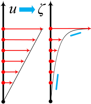
  $\zeta$ is dimensionless. Qualitatively, as sketched by figure 3, this envisioned transformation nonlinearly maps the velocity
  $u$-axis into a
  $\zeta$-axis in such a way that, for example, the part of the axis close to
  $u = 0$ is stretched and the part close to
  $u = U_{max}$ is compressed. Hence, the velocity
  $u$ in the resulting
  $\zeta$-axis increases nonlinearly (as
  $\zeta$ increases from 0 to 1), slower in the vicinity of
  $\zeta = 0$ but faster when it gets close to
  $\zeta =1$.

Figure 3. Schematic representation of the nonlinear transformation that maps the velocity  $u$ to a scaled velocity
  $\zeta$. (a) The velocity increases linearly as
  $u$ increases from 0 to
  $U_{max}$ in the
  $u$-axis. (b) After the transformation, the velocity increases in a nonlinear manner as
  $\zeta$ increase from 0 to 1: slower when
  $\zeta$ is closer to 0 while faster when
  $\zeta$ is closer to 1.
We can then transform (2.4) back with respect to the  $u$-axis:
 \begin{equation} \frac{{\partial {P_N}( {u,t} )}}{{\partial t}} = D{A^2}\frac{{{\partial ^2}{P_N}}}{{\partial {u^2}}} + DA\frac{{\partial A}}{{\partial u}}\frac{{\partial {P_N}}}{{\partial u}}, \end{equation}
where
 \begin{equation} A = \frac{{\partial u}}{{\partial \zeta }} \end{equation}
is the mathematical definition of the transformation (2.3), which is a centrepiece of our approach giving the mapping rule for velocity from  $u$ to
  $\zeta$:
 \begin{equation} \zeta ( u ) = \int_0^u \frac{1}{A} \, \textrm{d}u. \end{equation}
 Note that the specific form of the proposed nonlinear transformation, which is not known a priori, is represented by an explicit expression of the key function  $A$, or the mapping rule
  $\zeta (u)$. In order to find out the key function
  $A$ in (2.6) and (2.7), we compare (2.5) to the Fokker–Planck equation, which has recently been shown to be able to describe statistically the transport process of an ensemble of bedload particles (Furbish, Roseberry & Schmeeckle Reference Furbish, Roseberry and Schmeeckle2012b):
 \begin{equation} \frac{{\partial {P_N} ( {u,t} )}}{{\partial t}} ={-}\frac{\partial }{{\partial u}} [ {\mu ( u ){P_N}} ] + \frac{{{\partial ^2}}}{{\partial {u^2}}} [{k ( u ){P_N}} ]. \end{equation}
 In the above equation  $\mu$ (m s
 $^{-2}$) and
  $k$ (m
 $^2$ s
 $^{-3}$) are, respectively, known as the ‘drift velocity’ and the ‘diffusivity’ with respect to the velocity
  $u$. We expand and rewrite (2.8) in the following form:
 \begin{align} \frac{{\partial {P_N}( {u,t} )}}{{\partial t}} &= k \frac{{{\partial ^2}{P_N}}}{{\partial {u^2}}} + {c_1}\mu\frac{{\partial {P_N}}}{{\partial u}} - \left[ {\frac{{\partial \mu }}{{\partial u}}{P_N} + ( {1 + {c_1}} )\mu \frac{{\partial {P_N}}}{{\partial u}}} \right] \nonumber\\ &\quad +\left({\frac{{{\partial ^2}k}}{{\partial {u^2}}}{P_N} + 2\frac{{\partial k}}{{\partial u}}\frac{{\partial {P_N}}}{{\partial u}}}\right), \end{align}
where  $c_1$ is a constant.
For the equilibrium transport condition, the velocity p.d.f. does not change with time, under which circumstance (2.5) and (2.9) become
 \begin{equation} 0 = D{A^2}\frac{{{\partial ^2}{f_p}}}{{\partial {u^2}}} + DA\frac{{\partial A}}{{\partial u}}\frac{{\partial {f_p}}}{{\partial u}}, \end{equation}
 \begin{equation}0 = k\frac{{{\partial ^2}{f_p}}}{{\partial {u^2}}} + {c_1}\mu \frac{{\partial {f_p}}}{{\partial u}} - \left[{\frac{{\partial \mu }}{{\partial u}}{f_p} + ( {1 + {c_1}} )\mu \frac{{\partial {f_p}}}{{\partial u}}} \right] + \left({\frac{{{\partial ^2}k}}{{\partial {u^2}}}{f_p} + 2\frac{{\partial k}}{{\partial u}} \frac{{\partial {f_p}}}{{\partial u}}} \right), \end{equation}
where  $f_p$ is the temporally stationary p.d.f. of the particle velocity (i.e. the p.d.f.
  $f_p(u)$ does not change with time).
One possible set of relations for both equations in (2.10) describing the same process can be written as follows:
 \begin{equation} k = D{A^2}, \end{equation}
 \begin{equation}{c_1}\mu = DA\frac{{\partial A}}{{\partial u}}, \end{equation}
 \begin{equation}\frac{{\partial \mu }}{{\partial u}}{f_p} + ( {1 + {c_1}} )\mu \frac{{\partial {f_p}}}{{\partial u}} = 0, \end{equation}
 \begin{equation}\frac{{{\partial ^2}k}}{{\partial {u^2}}}{f_p} + 2\frac{{\partial k}}{{\partial u}}\frac{{\partial {f_p}}}{{\partial u}} = 0. \end{equation}
This set of equations can be solved to give
 \begin{equation} {c_1} = 1, \quad k = \int \frac{{{c_2}}}{{{f_p}^2}}\,\textrm{d}u, \quad \mu = \frac{{{c_2}}}{{2{f_p}^2}}, \end{equation}
and the important result
 \begin{equation} {A^2} = \frac{{{c_2}}}{D}\int f_p^{ - 2}\,\textrm{d}u, \end{equation}
relating the key function  $A$ to the temporally stationary particle velocity p.d.f.
  $f_p$, which is in accordance with the equilibrium transport conditions as assumed in previous studies (Fathel et al. Reference Fathel, Furbish and Schmeeckle2015; Liu et al. Reference Liu, Pelosi and Guala2019).
We take advantage of recent experimental measurements (Lajeunesse et al. Reference Lajeunesse, Malverti and Charru2010; Roseberry et al. Reference Roseberry, Schmeeckle and Furbish2012; Fathel et al. Reference Fathel, Furbish and Schmeeckle2015) and theoretical analyses (Furbish & Schmeeckle Reference Furbish and Schmeeckle2013; Fan et al. Reference Fan, Zhong, Wu, Foufoula-Georgiou and Guala2014) that have documented an exponential-like form for the particle velocity p.d.f.  $f_p(u)$. Hence, we assume that the velocity p.d.f. follows an exponential distribution
 \begin{equation} f_p ( u ) = \frac{1}{U}\exp \left( { - \frac{u}{U}} \right), \end{equation}
where  $U$ is the mean velocity. A value
  $U_{max}$ for the velocity maximum can be adopted in accordance with the near-bed flow velocity, representing a physical constraint on the maximum particle velocity. As demonstrated by Wu et al. (Reference Wu, Furbish and Foufoula-Georgiou2020),
  $U_{max}$ can be set as 30 cm s
 $^{-1}$ for the dataset of Fathel et al. (Reference Fathel, Furbish and Schmeeckle2015), and the particle hop processes are not sensitive to this value.
Substituting (2.14) into (2.13), we obtain an explicit expression for the function  $A$:
$A$:
 \begin{equation} A = \sqrt {\frac{{{c_2}}}{D} \int {f_p}^{ - 2}\,\textrm{d}u} = {\textrm{e}^{{u}/{U}}}\sqrt{\frac{{{U^3}{c_2}}}{{2D}}}, \end{equation}
which can be used to determine the rule for mapping the velocity  $u$ into
  $\zeta$ according to (2.7):
 \begin{equation} \zeta ( u ) = \int _0^u \frac{1}{A}\,\textrm{d}u = \sqrt{\frac{{2D}}{{U{c_2}}}} \left( {1 - {\textrm{e}^{ - {u}/{U}}}} \right). \end{equation}
 Recall that we define  $\zeta$ as a scaled quantity in the range of
  $[0,1]$, meaning that
 \begin{equation} {\left. {\zeta ( u )} \right|_{u = 0}} = 0, \quad {\text{and}}\quad {\left. {\zeta ( u )} \right|_{u = \infty }} = 1. \end{equation}
The former part of (2.17a,b) is automatically satisfied according to (2.16), while the latter implies that
 \begin{equation} \sqrt {\frac{{2D}}{{U{c_2}}}} = 1, \end{equation}
further simplifying (2.16) to
 \begin{equation} \zeta ( u ) = 1 - {\textrm{e}^{ - {u}/{U}}}. \end{equation}
 With the above obtained explicit expression for the velocity transformation, we can verify the hypothesis posed at the beginning of this subsection, i.e. a nonlinear transformation exists for the mapped velocity variations governed by a diffusion equation. Specifically, we mapped the experimentally measured particle velocity series into the  $\zeta$-axis system according to (2.19), which were then used to calculate the transformed particle velocity variations
  ${\rm \Delta} \zeta$ by taking the difference between successive velocities in the
  $\zeta$-axis. We illustrate in figure 4 that, as opposed to the results expressed in the
  $u$-axis (figure 2b), the transformed velocity variation
  ${\rm \Delta} \zeta$ can be relatively well approximated by a Gaussian distribution, verifying our hypothesis of modelling the velocity variation with respect to the
  $\zeta$-axis by the diffusion equation (2.4).

Figure 4. QQ plot illustrates how close the p.d.f. of transformed velocity variation  ${\rm \Delta} \zeta$ can be described by a normal distribution. Compared with results in figure 2(b), a normal distribution fits much better to
  ${\rm \Delta} \zeta$ instead of
  ${\rm \Delta} u$. This verifies our hypothesis that a nonlinear transformation exists for modelling the velocity variation with respect to the
  $\zeta$-axis by a diffusion equation, i.e. (2.4).
In figure 5 we display the p.d.f. of the measured velocity variation expressed in the  $\zeta$-axis. The Gaussian distribution reproducing the measurements, with fitted parameters of zero mean and standard deviation
  $\sigma \approx 0.18$, is superimposed in the figure. This allows us to determine the diffusion coefficient in (2.4) by
 \begin{equation} {\sigma ^2} = 2D{\rm \Delta} t, \end{equation}
which gives
 \begin{equation} D = 4\ {\textrm{s}^{ - 1}} \end{equation}
based on the time step of experimental measurements of  ${\rm \Delta} t$ = 1/250 s (the standard deviation is dimensionless, the same as the scaled velocity
  $\zeta$). Note that we determined the parameter
  $D$ using the transformed acceleration data (with respect to
  $\zeta$); however,
  $D$ can be alternatively estimated with measured hop distances and travel times, as we will demonstrate later in § 3.2.

Figure 5. Empirical p.d.f. of transformed velocity variation  ${\rm \Delta} \zeta$ and the fitted normal distribution. The fitted theoretical distribution in the figure has a zero mean and a standard deviation of
  $\sigma \approx 0.18$.
From a Lagrangian perspective, (2.4) describes how the velocity of the particle changes with time (i.e. follows the Gaussian random walk with respect to  $\zeta$), while the streamwise position of the particle is controlled by the corresponding velocity variations, which can simply be expressed by the following stochastic differential equation:
 \begin{equation} \textrm{d}x = u ( \zeta ) \, \textrm{d}t, \end{equation}
where  $x$ (m) is the streamwise position of the particle. To map the transformed velocity
  $\zeta$ back into
  $u$, we only need to solve the inverse function of (2.19):
 \begin{equation} u ( \zeta ) ={-} U \log ( {1 - \zeta} ). \end{equation}
Notice that (2.4) and (2.22) describe a non-stop transport process for the bedload particle (i.e. the particle is travelling with velocity variations and does not stop). This point is straightforward if we write down the discrete forms of (2.4) and (2.22), respectively, as
 \begin{equation} \zeta ( {t + {\rm \Delta} t} ) = \zeta ( t ) + R\sqrt{2D{\rm \Delta} t}, \end{equation}
 \begin{equation}x(t+{\rm \Delta} t) = x(t) - U\log ( {1 - \zeta} ) {\rm \Delta} t, \end{equation}
the form of which is commonly used in numerically simulating motions of a single particle in the Lagrangian perspective (i.e. Monte Carlo simulation). In (2.24) the time step  ${\rm \Delta} t$ needs to be small enough,
  $R$ is a normally distributed random variable with unit variance, and the overall number of runs of the simulation needs to be large enough. Each run of the simulation provides the trajectory of a single particle, and the ensemble of runs provides statistical information on the motions of bedload particles. It is seen that, without specifying a condition for the cessation of the particle motion for (2.24), a simulated particle is always travelling and does not stop, which we refer to as a ‘non-stop transport process’.
The Lagrangian form of (2.24) is more intuitive in describing the physical process of bedload particle transport. However, for convenience in obtaining analytical solutions, we can switch back to the Eulerian description for (2.24), which turns out to be (Dimou Reference Dimou1989; Ancey & Heyman Reference Ancey and Heyman2014; Li et al. Reference Li, Aubeneau, Bolster, Tank and Packman2017)
 \begin{equation} \frac{{\partial {P_N} ( {x,\zeta ,t} )}}{{\partial t}} = U\log ( {1 - \zeta } )\frac{{\partial {P_N}}}{{\partial x}} + D\frac{{{\partial ^2}{P_N}}}{{\partial {\zeta ^2}}}, \end{equation}
where  ${P_N}( {x,\zeta ,t} )$ is now the joint p.d.f. of the streamwise position
  $x$, the velocity (with respect to
  $\zeta$) and the time
  $t$. The subscript
  $N$ further stands for the non-stop process.
Obtaining  $\langle P_N \rangle$ with respect to
  $\zeta$ gives the joint p.d.f. of streamwise position and time, where the angle brackets are defined as
 \begin{equation} \langle\,{\cdot}\,\rangle = \int _0^1 (\,{\cdot}\,) \, \textrm{d}\zeta. \end{equation}
2.3. Description of the bedload particle hops by the obtained governing equation
As noted above, without additional constraints, (2.25) represents a non-stop process (the particle never stops its motion during the transport). However, particles move through a sequence of hops during which they must start and stop their motions with zero velocity. To perform a hop, a particle first starts its motion from a stationary position, which can be used to set the initial condition for (2.25) as
 \begin{equation} P{|_{t = 0}} = \delta ( x ) \delta ( {\zeta - {\zeta _0}} ), \end{equation}
where  $\delta (\,{\cdot }\,)$ is the Dirac delta function. In this section (§ 2.3), we are imposing constraints aimed at connecting the previously discussed non-stop transport process to the particle hop. To distinguish between the two processes, hereafter we use the notation of
  $P(x, \zeta , t)$ for the particle hop that is delimited by two resting periods, compared with that of
  $P_N(x, \zeta , t)$ for the non-stop process.
Equation (2.27) implies that we ignore when and where particles are performing these hops (Wu et al. Reference Wu, Furbish and Foufoula-Georgiou2020), under which circumstance we can virtually move the starting position of all hops to the same place and allow particles to move at the same time. Specifically, (2.27) states that particles start to move at the time  $t = 0$, from the streamwise location
  $x=0$, and with a velocity of
  $u=u(\zeta _0)$; additionally, applying
  $\zeta _0\rightarrow 0$ gives the initial velocity of
  $u=0$, defining the transition between rest and motion regimes, consistent with the phenomenology of particle hops during the entrainment phase.
During travelling, particles’ velocities are confined between the minimum and maximum values:
 \begin{equation} \left.\frac{{\partial P}}{{\partial \zeta }}\right|_{\zeta = 0} = \left.\frac{{\partial P}}{{\partial \zeta }}\right|_{\zeta = 1} = 0. \end{equation}
 A moving particle must stop its motion to complete a hop. Experimental studies have suggested that the time for a bedload particle to remain in motion (i.e. the travel time  $\tau$) follows an exponential distribution (Martin et al. Reference Martin, Jerolmack and Schumer2012; Roseberry et al. Reference Roseberry, Schmeeckle and Furbish2012; Fathel et al. Reference Fathel, Furbish and Schmeeckle2015; Liu et al. Reference Liu, Pelosi and Guala2019), implying a memoryless process for the termination of the particle hop (Martin et al. Reference Martin, Jerolmack and Schumer2012). To incorporate such a memoryless process into the governing equation, we can add a sink term with the particle deposition rate
  $k_a$ (s
 $^{-1}$ ) for the non-stop transport process (2.25):
 \begin{equation} \frac{{\partial P ( {x,\zeta ,t} )}}{{\partial t}} = U\log ( {1 - \zeta } )\frac{{\partial P}}{{\partial x}} + D\frac{{{\partial ^2}P}}{{\partial {\zeta ^2}}} - {k_a}P. \end{equation}
Again, we note that we have dropped the subscript  $N$ and use
  $P(x, \zeta , t)$ for particle hops as first introduced in (2.27). The sink term in (2.29) indicates that the cessation of a particle's motion (thus completing the hop) is an independent, random event, resulting in an exponential distribution for the travel times (Zeng & Chen Reference Zeng and Chen2011).
It is easy to perform numerical simulations to extract particle hops using (2.24), based on the above discussed constraints. However, from an Eulerian perspective, we note that the solution of (2.29),  $P({x,\zeta ,t})$, does not directly correspond to the hop events. We emphasize the fact that
  $P( {x,\zeta ,t} )$ describes the spatial–temporal (and velocity) evolution for the active particles. Such particles have started from zero velocity by considering the initial condition (2.27) but have not yet stopped their motions; because, once they stop, they will no longer be represented by
  $P$. Thus, the deduced mean travel distance
  $L(t)$ based on
  $P( {x,\zeta ,t} )$ does not represent the mean hop distance of particles (denoted as
  $L_h(\tau )$ and conditional on particles that have ceased their motions at the time
  $\tau$), since these particles are still moving and have not stopped at time
  $t$.
$t$.
In order to bridge the gap between the two processes so as to use the solution of (2.29) to obtain the mean hop distance–travel time relation ( $L_h$–
 $\tau$), we consider an in-between time
  $t_0$ during a particle hop (
 $0\leq t_0 \leq \tau$), as sketched in figure 6(a). Consequently, the mean distance travelled by the active particles
  $L( t_0 )$ can be obtained as the solution of (2.29) with respect to
  $t_0$. A further relation between
  $t_0$ and
  $\tau$, and between
  $L( t_0 )$ and
  $L_h( \tau )$, may enable us to ‘translate (or extend)’ the result of
  $L( t_0 )$ to obtain
  $L_h( \tau )$.

Figure 6. (a) Sketch for particle hops with the same travel time  $\tau$. Note that the hop/travel distance is an average for an ensemble of particle hops. (b)Mean hop/travel distances calculated based on travel times of particle hops for 0.04 s increments, up to 0.36 s. It is seen that the assumption of
  $L_h(\tau ) = 2L(t_0)$ is well supported by empirical data for hops under different travel times, which is critical to ‘translate’ the solution of (2.29) to obtain the mean hop distance–travel time relation (
 $L_h$–
 $\tau$).
Motivated by the intuitive understanding of ‘symmetry’ for the trajectory of particle hops in an ensemble average sense (i.e. at the initial stage the particle generally accelerates, and before the cessation of motion it generally decelerates), we expect that, for hops with the same travel time: by the ‘half travel time’  $t_0= \tau /2$, on average they travel half of the mean hop distance,
 \begin{equation} L_h ( \tau ) = 2L ( t_0 )|_{t_0\equiv \tau/2}. \end{equation}
 We used empirical data to verify the assumption of (2.30). Using the time interval of 0.04 s (i.e. 10 ${\rm \Delta} t$) and setting nine successive time intervals of [
 $0.04 (i-1), 0.04 i$] (s), where
  $i= 1, 2, 3,\ldots , 9$, we divided particle hops into different groups according to their travel times
  $\tau$. For every group of particle hops, we calculated the mean hop distance
  $L_h(\tau )$ and the mean travel distance
  $L(t_0)$ (i.e. found the distance travelled during half of the travel time for every hop, and then calculated the mean over the group of hops). Note that only fewer than 5 % of particle hops travel longer than
  $10{\rm \Delta} t = 0.36$ s, too few to guarantee the convergence for the mean hop distances at longer travel-time intervals. Those hops were not included in the analysis. We display the results in figure 6(b), demonstrating an excellent support to the assumption of (2.30) for either short or long hops. In § 3 we will analytically solve (2.29) for the mean travel distance
  $L(t_0)$, and then ‘translate’ the results based on (2.30) to obtain the mean hop distance–travel time relation (
 $L_h$–
 $\tau$).
3. Results and discussion
We note that the advection–diffusion equation, (2.25), is exactly in the form of the governing equation for a Taylor dispersion process (Taylor Reference Taylor1953), which describes the transport of a solute substance in laminar shear flows. We recall that the flow shear, imposing a spatial difference of streamwise velocities, contributes to the streamwise separation (scattering) of solute molecules (Wu & Chen Reference Wu and Chen2014). The original concept of Taylor dispersion describes the solute molecules performing a Gaussian random walk in a real spatial dimension (e.g. vertically, across the water depth) where they experience different streamwise flow velocities. As a comparison, with (2.25) we envision a virtual velocity dimension  $\zeta$ for the bedload particle to perform the Gaussian random walk, during which its streamwise velocity varies by continuously sampling the ‘shear flow profile’ represented by (2.23). Analytical techniques for studying Taylor dispersion can thus be applied to further analyse the bedload transport process.
3.1. Analytical solutions
For the advection–diffusion equation (2.29) with a sink term, it is known that its solution can be expressed as the product of an exponential decay term and the solution of a corresponding non-stop transport process as given by (2.25) (Zeng & Chen Reference Zeng and Chen2011):
 \begin{equation} P ( {x,\zeta ,t_0} ) = {P_N} ({x,\zeta ,t_0} )\exp ( { - {k_a}t_0} ). \end{equation}
From a particle-tracking perspective, (3.1) indicates that, while the motion of the particle is governed by a non-stop process (i.e.  $P_N$), the probability for this particle to continue its motion after each time step is determined by an exponential function
  $\exp (-k_a{\rm \Delta} t_0)$ until the particle stops.
Based on the knowledge of Taylor dispersion, we understand that (2.25) cannot be analytically solved for  $P_N$, but, instead, that statistical information regarding the bedload particle hops can be obtained through solving the corresponding moment equations (Aris Reference Aris1956). In fact, (3.1) allows us to define the
  $p$th-order moment of
  $P(x,\zeta ,t_0)$ as
  $M_p (\zeta ,t_0)$:
 \begin{equation} {M_p} ( {\zeta ,t_0} ) = {m_p} ( {\zeta ,t_0} )\exp( { - {k_a}t_0} ), \end{equation}
where
 \begin{equation} {m_p} ( {\zeta ,t_0} ) = \int _{ - \infty }^{ + \infty } {P_N} ( {x,\zeta ,t_0} ){x^p} \, \textrm{d}x \end{equation}
is the  $p$th-order moment for the non-stop bedload transport (
 $p = 0, 1, 2, \ldots$).
In this work, we consider only the first two statistical moments (i.e.  $p = 0$ and 1), which are sufficient for studying the bedload particle hops. As we are going to demonstrate below, the zeroth-order moment
  $M_0 (\zeta ,t_0)$ is associated with the travel-time distribution of particle hops; and the first-order moment
  $M_1 (\zeta ,t_0)$ specifies the mean hop distance–travel time relation (
 $L_h$–
 $\tau$). Currently, there is only one undetermined parameter (
 $k_a$), i.e. the deposition rate in (2.29), which can be fitted to the measured data of travel-time p.d.f. when we solve for the zeroth-order moment
  $M_0 (\zeta ,t_0)$. Although the diffusion coefficient
  $D$ is already obtained in (2.21) by considering the p.d.f. of the transformed velocity variation
  ${\rm \Delta} \zeta$, we will demonstrate below how it can be determined alternatively by experimental measurements of travel times and mean hop distances, as a further validation of our theoretical framework.
Applying the operation  $\int _{-\infty }^{+\infty }(\,{\cdot }\,){x^p}\,\textrm {{d}}x$ to (2.27)–(2.29), we can obtain the zeroth- and first-order moment equations (i.e.
  $p = 0$ and 1), respectively, as
 \begin{equation} \frac{{\partial {m_0}( {\zeta ,t_0} )}}{{\partial t_0}} = D\frac{{{\partial ^2}{m_0}}}{{\partial {\zeta ^2}}}, \end{equation}
 \begin{equation}\frac{{\partial {m_1}( {\zeta ,t_0} )}}{{\partial t_0}} = D\frac{{{\partial ^2}{m_1}}}{{\partial {\zeta ^2}}} - U\log ( {1 - \zeta } ){m_0} ( {\zeta ,t_0} ), \end{equation}
with their initial conditions
 \begin{equation} {m_p} ( {\zeta ,t_0} ){|_{t_0 = 0}} = \begin{cases} \delta ( {\zeta - {\zeta _0}} ), & {p = 0} ,\\ 0, & {p = 1} , \end{cases} \end{equation}
and corresponding boundary conditions
 \begin{equation} \left.\frac{{\partial {m_p}}}{{\partial \zeta }}\right|_{\zeta = 0} = \left.\frac{{\partial {m_p}}}{{\partial \zeta }}\right|_{\zeta = 1} = 0. \end{equation}
 Considering  $\zeta _0\rightarrow 0$ (bedload particles start their motions with a velocity of
  $u=0$), the zeroth-order moment in (3.4) can be solved as
 \begin{equation} {m_0} ( {\zeta ,t_0} ) = 1 + 2\sum_{n = 1}^\infty \cos ( {{\beta _n}\zeta } ){\textrm{e}^{ - D\beta _n^2t_0}}, \end{equation}
where  $\beta _n=n {\rm \pi},\ n=1, 2, 3, \ldots\,$.
It is obvious that
 \begin{equation} \langle {{m_0} ( {\zeta ,t_0} )} \rangle = 1 \quad \textrm{and}\quad \langle {{M_0} ( {\zeta ,t_0} )} \rangle = {\textrm{e}^{ - {k_a}t_0}}, \end{equation}
indicating that the number of bedload particles in motion remains the same for non-stop bedload transport, but decays exponentially due to deposition which terminates particle hops. Note that  $(1-\langle {{M_0}( {\zeta ,t_0} )} \rangle )$ gives the temporal evolution of the probability that the particle has ceased its motion, which is precisely the definition of the cumulative distribution function (c.d.f.) of the travel time for particle hops. Thus, the corresponding p.d.f. can be analytically determined by differentiating it with respect to the time variable
  $t_0$:
 \begin{equation} {f_T} ( t_0 ) = \frac{\textrm{d}}{{\textrm{d}t_0}} ( {1 - \langle {{M_0} ( {\zeta ,t_0} )} \rangle } ) = {k_a}{\textrm{e}^{ - {k_a}t_0}}. \end{equation}
 Recall that  $t_0$ stands for only half of the travel time (i.e.
  $t_0 = \tau /2$) based on (2.30). When considering the p.d.f. for the entire travel period, (3.9) should be modified as
 \begin{equation} {f_T} ( \tau ) = ({k_a}/2 ){\textrm{e}^{ - {k_a}\tau /2}}, \end{equation}
which is an exponential distribution, agreeing with the form observed in experiments (Martin et al. Reference Martin, Jerolmack and Schumer2012; Fathel et al. Reference Fathel, Furbish and Schmeeckle2015; Liu et al. Reference Liu, Pelosi and Guala2019). The mean travel time of the above p.d.f. is  $2/k_a$, where the parameter
  $k_a$ can be determined based on the experimental measurements. For example, Fathel et al. (Reference Fathel, Furbish and Schmeeckle2015) calculated the mean travel time for the particle-tracking experiment as 0.12 s, giving
  $k_a =16.67$ s
 $^{-1}$. Equation (3.10) will be used later to determine the analytical solution for the hop-distance distribution.
We note that the physical meaning of the normalized first-order moment (by the proportion of moving particles, here  $\langle {{M_0}} \rangle$) is the mean streamwise displacement of bedload particles at a given time, i.e. the mean travel distance of particles with the same half travel time
  $t_0$. Thus,
  $\langle {{M_1}} \rangle / \langle {{M_0}} \rangle$ eventually gives the mean hop distance–travel time relation (
 $L_h$–
 $\tau$) according to (2.30). Applying the average operator defined in (2.26) on both sides of the first-order moment equation, (3.4b), we obtain
 \begin{equation} \frac{{\partial \langle {{m_1}} \rangle }}{{\partial t_0}} ={-} U \langle {\log ( {1 - \zeta } ){m_0} ( {\zeta ,t_0} )} \rangle , \end{equation}
which can be solved based on the solution of  $m_0$ in (3.7), leading to
 \begin{align} L(t_0) &= \langle {{M_1}} \rangle / \langle {{M_0}} \rangle = \langle {{m_1}} \rangle / \langle {{m_0}} \rangle \nonumber\\ &=Ut_0 + 2U\sum _{n = 1}^\infty \frac{{1 - {\textrm{e}^{ - D\beta _n^2t_0}}}}{{D\beta _n^3}}\cos ( {{\beta _n}} )\textrm{Si} ( {{\beta _n}} ), \end{align}
where Si $(\,{\cdot }\,)$ is the sine integral function
 \begin{equation} \textrm{Si} ( {{\beta _n}} ) = \int_0^{{\beta _n}} ({ \sin ( z )}/z ) \, \textrm{d}z. \end{equation}
 Again, we note that  $t_0$ is only half of the travel time (i.e.
  $t_0 = \tau /2$); for the entire particle hop, according to (2.30) we have
 \begin{align} L_h(\tau)&= 2L(t_0)= 2L(\tau/2) \nonumber\\ &=U\tau + 4U\mathop \sum _{n = 1}^\infty \frac{{1 - {\textrm{e}^{ - D\beta _n^2\tau /2}}}}{{D\beta _n^3}}\cos ({{\beta _n}} )\textrm{Si} ( {{\beta _n}} ), \end{align}
which gives the analytical solution for the mean hop distance of an ensemble of particles ( $L_h$) as a function of the travel time (
 $\tau$).
3.2. Mean hop distance–travel time scaling for short and long particle hops
One observation regarding (3.14) is that for long-hop bedload particles ( ${\tau \to \infty }$), the mean hop distance scales linearly with the travel time:
 \begin{equation} L_h ( \tau ){|_{\tau \to \infty }} = U\tau + 4U\mathop \sum _{n = 1}^\infty \frac{{\cos ( {{\beta _n}} )\textrm{Si} ( {{\beta _n}} )}}{{D\beta _n^3}}\sim \tau. \end{equation}
 This asymptotic regime was discovered recently (Wu et al. Reference Wu, Furbish and Foufoula-Georgiou2020) as a correction to previous studies proposing a single regime for the hop-distance scaling (with an exponent of  $\sim 2$ or
  $\sim 5/3$) of bedload particle motions (Roseberry et al. Reference Roseberry, Schmeeckle and Furbish2012; Fathel et al. Reference Fathel, Furbish and Schmeeckle2015). The scaling regime of
  $L_h \sim \tau$ was physically explained by resorting to the earlier formulation by Ancey & Heyman (Reference Ancey and Heyman2014) based on the mean-reverting process, which is valid for the description of long-hop particles (Wu et al. Reference Wu, Furbish and Foufoula-Georgiou2020). Under the present formulation invoking Taylor dispersion theory, this linear scaling regime is simply known as the Taylor dispersion regime, when the particle has sampled many times possible velocities within the ‘shear velocity profile’, (2.23). The quote marks represent that it is only mathematically in the same form of the Taylor dispersion process. This understanding indicates that the mean velocity of particle hops converges to a constant
  $U$ by the time scale
  $1/D$, where the constant 1 is brought by the normalized velocity
  $\zeta$. By merely examining the asymptotic regime of the particle hops, i.e. computing the mean velocity of long hops and estimating the starting time of this asymptotic regime, we can roughly estimate the necessary parameters for the governing equation. This point will be further elaborated in later discussion.
As also noted by Wu et al. (Reference Wu, Furbish and Foufoula-Georgiou2020), so far there exists no theory to explain the scaling regime for the short-hop particles, though intuitively it may be attributed to the large proportion of acceleration and deceleration (entrainment and deposition) periods over the entire travel time (of the hop). Owing to the lack of theoretical guidance, and the complicated patterns of short hops, different exponents for the initial scaling regime have been estimated in the literature, and no consensus has been reached for a possibly unified constant. For example, the exponent of 5/3 first appeared in the analysis of a portion of the experimental data by Roseberry et al. (Reference Roseberry, Schmeeckle and Furbish2012) (figure 13 in their paper), most of which are now seen for short hops. With much larger datasets used in a reanalysis, Fathel et al. (Reference Fathel, Furbish and Schmeeckle2015) proposed a new exponent of 2 based on a first estimate of the hop distance–travel time plot (figure 10 in their paper). And this exponent was followed for short hops in the recent study (Wu et al. Reference Wu, Furbish and Foufoula-Georgiou2020) focusing on scaling regime shifts for particle motions.
While (3.14) does not seem to offer an explicit scaling exponent for the short hops, this analytical solution gives us much more detailed and consistent information compared with numerical simulations (Wu et al. Reference Wu, Furbish and Foufoula-Georgiou2020). In figure 7(a) we present results of (3.14) using three different values of the diffusion coefficient  $D$, respectively, 100, 10 and 1 s
 $^{-1}$. The first observation is that different values of
  $D$ do not affect the long-time asymptotic regime, which agrees with the theoretical expectation of (3.15). However, the time needed for such a transition to the long-time approximation increases as
  $D$ decreases, which is related to the characteristic time scale
  $1/D$ by Taylor dispersion theory. Taking the blue curve as an example (for
  $D = 100$ s
 $^{-1}$), we can see that one more scaling transition occurred for travel times shorter than
  $1/D$, as indicated by the two blue solid reference lines with different slopes, which can be used to estimate the scaling exponents as
  $\sim 1.5$ and
  $\sim 5/3$, respectively. We can argue that the time scale of
  $0.1/D$ sets the upper limit of travel times for the initial regime with the scaling exponent of 1.5. This means that particles have a slow mean velocity when starting the hop, which can increase as
  $\sim \tau ^{0.5}$ if the particle is able to travel longer during a hop. The time scales in between
  $(0.1/D, 1/D)$ suggest a transition regime. Particle hops with duration falling within the initial and transition regimes can all be defined as short hops, since the mean velocity of these hops has not reached a constant. We note that these scaling regimes could not be identified without the help of the analytical solution of (3.14), given fluctuations and uncertainties observed in numerical and experimental results as shown by figure 4(b) in the paper of Wu et al. (Reference Wu, Furbish and Foufoula-Georgiou2020). The effect of
  $U$ is more straightforward, as it sets the mean velocity for the long-hop particles (and can thus be determined by the experimental measurements), according to (3.15).

Figure 7. Scaling regimes for mean hop distances ( $L_h$) and travel times (
 $\tau$) of bedload particle hops. (a) Effects of diffusion coefficient
  $D$, with two characteristic times of
  $0.1/D$ and
  $1/D$ marked for the blue curve of
  $D = 100$ s
 $^{-1}$ indicating three stages, respectively, as an initial, a transition and the Taylor dispersion regime. (b) Comparison between the experimental data (Fathel et al. Reference Fathel, Furbish and Schmeeckle2015) for the mean hop distances, which is the same as that presented in figure 4(b) by Wu et al. (Reference Wu, Furbish and Foufoula-Georgiou2020), and the analytical solution (3.14) with parameters of
  $D = 4$ s
 $^{-1}$ and
  $U = 5.56$ cm s
 $^{-1}$.
The above discussion provides guidelines for estimating the parameters necessary for particle motions in the governing equation (2.29) using measurements of hop distances and travel times. Based on the experimental data (Fathel et al. Reference Fathel, Furbish and Schmeeckle2015) for long hops, we can estimate  $U=5.56$ cm s
 $^{-1}$. It can also be observed from the experimental data that the Taylor dispersion regime for particle hops starts approximately between 0.2 and 0.3 s (Wu et al. Reference Wu, Furbish and Foufoula-Georgiou2020), which gives an estimation of the diffusion coefficient
  $D$ in the range from 3.33 to 5 s
 $^{-1}$. Additionally, fitting (3.14) to measured data of the mean hop distances at different travel times, we can determine the diffusion coefficient
  $D$. Note also that our first estimated value of
  $D = 4$ s
 $^{-1}$ in (2.21) based on the p.d.f. of the transformed velocity variation
  ${\rm \Delta} \zeta$ falls right in the 3.33 to 5 s
 $^{-1}$ range, corresponding to the average of 0.2 and 0.3 s for
  $1/D$. The effect of the diffusion coefficient
  $D$ on the particle motions can be phenomenologically interpreted by considering D as a measure of how fast the particle can change its velocity during the transport. Thus, the faster the particle samples different velocities from the ‘shear velocity profile’ of (2.23) in a Gaussian random walk manner (measured by the standard deviation of the p.d.f. of
  ${\rm \Delta} \zeta$), the shorter time it needs to experience these velocities many times to approach the Taylor dispersion regime for long hops.
In figure 7(b), we show that the calculated red points for mean hop distances with respect to travel times from the experimental data are perfectly captured by the solid line representing the analytical solution of (3.14). Since the transition regime for the experimental data starts around  $0.1/D = 0.025$ s, it can be seen that an exponent larger than 1.5 (here 5/3) explains quite a portion of the scaling behaviour for the measured short hops (mostly in the transition regime), providing a theoretical basis for the estimation of 5/3 made by Roseberry et al. (Reference Roseberry, Schmeeckle and Furbish2012). Note also that the present formulation may explain the estimates of lower exponents (in the range 1.25–1.30) as provided from the experiments by Liu et al. (Reference Liu, Pelosi and Guala2019) in similar transport conditions.
Along with the deposition rate of  $k_a =16.67$ s
 $^{-1}$ as appeared in equation (3.10), all parameters required in the governing equation (2.29) are now determined. We highlight that, based on the diffusion coefficient
  $D = 4$ s
 $^{-1}$ and our demarcation on particles performing short hops (i.e. the travel time
  $\tau < t_s$, with the characteristic time
  $t_s = 1/D$), for the Fathel et al. (Reference Fathel, Furbish and Schmeeckle2015) experimental dataset, the number of short hops covers over 84 % of the entire hop events according to the travel-time distribution described by (3.10).
3.3. Hop-distance distributions
The hop distance has long been regarded as a key random variable in the formulation of bedload sediment transport, and the form of its distribution is thus of both theoretical and practical importance. Conventionally, the calculation of sediment flux is based on the mean hop distance under equilibrium transport conditions (Einstein Reference Einstein1950), while the second-order moment of the hop-distance distribution comes into play for more generalized cases (Furbish et al. Reference Furbish, Haff, Roseberry and Schmeeckle2012a). Regarding formulations on bedload tracer transport, where an ensemble of tracer particles is followed during the course of experimental observation, the mean of the hop-distance distribution is necessary for the advective term of the tracer transport, whereas the variance contributes to the streamwise diffusion of tracers (Ganti et al. Reference Ganti, Meerschaert, Foufoula-Georgiou, Viparelli and Parker2010; Wu et al. Reference Wu, Foufoula-Georgiou, Parker, Singh, Fu and Wang2019a,Reference Wu, Singh, Fu and Wangb).
The analytical solution of  $L_h(\tau )$ for the mean hop distance–travel time relation allows us not only to distinguish between different transport regimes of particle motions depending on how long the particle can travel during a single hop, but also to straightforwardly and theoretically address the specific form of the hop-distance distribution. Based on the work of Fathel et al. (Reference Fathel, Furbish and Schmeeckle2015) (equation (B1) in their paper) and (3.10) for the travel-time distribution
  $f_T$, we have
 \begin{equation} {f_L} ( x ) = \left| {\frac{{\textrm{d}{L^{ - 1}}( x )}}{{\textrm{d}x}}} \right| \, {f_T}\left( {{L^{ - 1}} ( x )} \right) = \left| {\frac{{\textrm{d}{L^{ - 1}}( x )}}{{\textrm{d}x}}} \right| \frac{{{k_a}}}{2}\exp\left( { - \frac{{{k_a}}}{2}{L^{ - 1}} ( x )} \right). \end{equation}
 In the above equation,  $L^{-1} (x)$ is the inverse function of
  $L_h(\tau )$, which cannot be given explicitly, but can be calculated numerically according to (3.14). In figure 8 we compare the theoretical result of the hop-distance distribution (3.16) with the experimental measurements, based on the obtained parameters
  $D$,
$D$,  $U$ and
  $k_a$. The good agreement serves as an excellent validation of the formulation in (2.29) for bedload particle hops. In addition, as also pointed out by Wu et al. (Reference Wu, Furbish and Foufoula-Georgiou2020), the emerging mixed form of the hop-distance distribution, a Weibull-like front and an exponential-like tail, is the result of the different transport regimes for short- and long-hop particles, respectively. That is, the linear scaling of
  $L_h(\tau ) \sim \tau$ for long hops ensures that the tail of the hop-distance p.d.f. is the same as that of the travel times, which is an exponential distribution. And the scaling of
  $L_h(\tau ) \sim \tau ^2$ for short hops implies that a different form than the exponential distribution, specifically the Weibull distribution, will emerge for small hop distances in the p.d.f., as concluded by Fathel et al. (Reference Fathel, Furbish and Schmeeckle2015). We note that the tail characteristics of the hop-distance p.d.f. is important in the sense that the heavy-tailed distribution of hop distances was proposed as a possible reason for the observed anomalous diffusion of bedload particle transport (Schumer, Meerschaert & Baeumer Reference Schumer, Meerschaert and Baeumer2009). Thus the thin-tailed distribution of hop distances should indicate the existence of different mechanisms leading to the anomalous diffusion, which, for example, can be related to the heavy-tailed waiting time distribution caused by tracer particles when they stop moving and/or get buried (Liu et al. Reference Liu, Pelosi and Guala2019; Wu et al. Reference Wu, Foufoula-Georgiou, Parker, Singh, Fu and Wang2019a,Reference Wu, Singh, Fu and Wangb).

Figure 8. The p.d.f. of bedload particle hop distance. (a) Comparison between the experimental data (Fathel et al. Reference Fathel, Furbish and Schmeeckle2015) and the theoretical result of (3.16). The inset shows the same results presented in linear–log plot. (b) Analytical solution for the hop-distance distribution of long hops, in contrast to the Weibull-like front of the distribution for short hops. If there exist only long hops, (3.18) should shift vertically and approach (3.19), which is the exponential p.d.f. for hop-distances conventionally adopted by Einstein (Reference Einstein1950) and others in their research.
In fact, under the current formulation for an exponential distribution of travel times, we can further obtain an explicit expression for the tail of the hop-distance distribution according to the transport regime of the bedload particle performing long hops. Based on the linear relation in (3.15), we have
 \begin{equation} {L^{ - 1}} ( x ){|_{x \to \infty }}= \frac{1}{U}x - 4\sum _{n = 1}^\infty \frac{{\cos ( {{\beta _n}})\textrm{Si} ( {{\beta _n}} )}}{{D\beta _n^3}}, \end{equation}
which results in
 \begin{equation} {f_L} ( x ){|_{x \to \infty }}=\frac{{{k_a}}}{{2U}}\exp \left( { - \frac{{{k_a}}}{{2U}}x + 2{k_a}\sum _{n = 1}^\infty \frac{{\cos ( {{\beta _n}} )\textrm{Si}( {{\beta _n}})}}{{D\beta _n^3}}} \right), \end{equation}
indicating an exponential tail of the distribution, agreeing with our qualitative description. According to (3.16), the linear relation of (3.17) simply tells us that the form of the tail of the hop-distance distribution must be the same as that of the travel-time distribution (consistent with observations by Roseberry et al. Reference Roseberry, Schmeeckle and Furbish2012; Liu et al. Reference Liu, Pelosi and Guala2019).
In figure 8(b) we can see that (3.18) captures well the exponential tail of the hop-distance distribution. The Weibull distribution (blue line) in the figure is adopted from Fathel et al. (Reference Fathel, Furbish and Schmeeckle2015):  ${f_{LW}}( x ) = \sqrt {{x^{ - 1}}/\langle x\rangle /2} \, \exp ({-\sqrt {2/\langle x\rangle } \, {x^{1/2}}} )$, with the measured mean hop distance
  $\langle x\rangle = 0.46$ cm. The small differences for short hops between the Weibull distribution and the results of (3.16) are due to different scaling exponents (e.g. 5/3 or 2 for the transition regime) for the mean hop distance–travel time relation. To account for the sharp decay of the probability density by the Weibull-like front due to the large number of particles performing short hops, the black solid line representing (3.18) has to be shifted downwards in the figure as compared with the following exponential p.d.f.:
 \begin{equation} {f_{Le}} ( x )=\frac{{{k_a}}}{{2U}}\exp \left( { - \frac{{{k_a}}}{{2U}}x} \right). \end{equation}
Note that (3.19) is only for long hops (i.e. hops with a constant mean velocity), and represents the classic form of hop-distance distribution as assumed by Einstein (Reference Einstein1950) and following studies (Paintal Reference Paintal1971; Wu et al. Reference Wu, Foufoula-Georgiou, Parker, Singh, Fu and Wang2019a).
3.4. Validation based on the acceleration distribution
As a further validation of our formulation for the bedload particle hops, we numerically calculated the p.d.f.s of the particle accelerations by particle-tracking simulations based on (2.25). By the algorithm of Gaussian random walk on the  $\zeta$-axis (2.24a), and the inverse rule for mapping velocity from
  $\zeta$-axis to
  $u$-axis (described by (2.23)), we can generate a time series of velocity
  $u$ for a particle in motion with the time step of
  ${\rm \Delta} t = 0.004$ s, which is the same as the interval used for data sampling in experimental measurements. Note that
  $R$ in (2.24a) is a normally distributed random variable with zero mean and unit standard deviation. The initial and boundary conditions for (2.24a) during the simulations are defined by (2.27) and (2.28), respectively. The same parameter of
  $D = 4$ s
 $^{-1}$ is used for the simulation. The accelerations are then obtained by
  ${\rm \Delta} u /{\rm \Delta} t$, and the results of our theoretical framework agree well with the measurements by Fathel et al. (Reference Fathel, Furbish and Schmeeckle2015) (figure 9). We note that simulated particle accelerations have not been constrained during the formulation of bedload particle hops in this paper (i.e. (2.29)). Hence, the emerging Laplace form of the acceleration p.d.f. is an independent validation and it is also consistent with recent measurements by Liu et al. (Reference Liu, Pelosi and Guala2019).

Figure 9. Comparison of acceleration p.d.f.s between the experimental data (Fathel et al. Reference Fathel, Furbish and Schmeeckle2015) and results of numerical simulation based on the proposed theoretical framework. The Laplace distribution in the figure (blue line) is  $f( {{a_x}} ) = ({1}/{{2\lambda }})\exp ( { - {{| {{a_x}} |}}/{\lambda }} )$, where
  $a_x$ is the acceleration (cm s
 $^{-2}$ ) and the parameter
  $\lambda =610$ cm s
 $^{-2}$.
We also note that the Laplace-like p.d.f. for the accelerations in figure 9 is not the result of the exponential-like velocity distribution (as we have assumed in (2.14)). We emphasize that, if the particle velocity is randomly drawn each time from the exponential p.d.f. of (2.14) to construct the velocity trajectory as shown by figure 1, the resulting acceleration p.d.f. is indeed Laplace, but with a different variance compared with the results in figure 9. We have performed such numerical simulations to generate the acceleration p.d.f. as demonstrated in figure 10, which is evidently different from the results in figure 9. This can be attributed to the fact that  ${\rm \Delta} \zeta$ (difference of nonlinearly transformed velocities) in our model is generated by a normally distributed random variable
  $R$ as seen in (2.24a), instead of the difference between two velocities randomly drawn from the exponential p.d.f. of (2.14), respectively.

Figure 10. Demonstration that the acceleration p.d.f. in figure 9 is not the result of the exponential distribution of (2.14). The fitted Laplace distribution (red line) to the simulated accelerations in this figure has a very different variance compared to the Laplace p.d.f. in figure 9 (also reproduced here as the blue line). This is because the numerically simulated accelerations were obtained by differences of two velocities each randomly drawn from the exponential distribution of (2.14), rather than that generated by a normally distributed random variable  $R$ as seen in (2.24a) and presented in figure 9.
4. Conclusions
In this paper, we investigate the experimental data and find that the velocity variations  ${\rm \Delta} u$ during particle hops do not follow a Gaussian random walk process. Instead, by performing a nonlinear transformation and mapping the velocity
  $u$ into an opportunely distorted velocity axis
  $\zeta$, the corresponding velocity variation
  ${\rm \Delta} \zeta$ can be approximated by a Gaussian random walk process, which is equivalent to a governing diffusion equation with respect to the new variable
  $\zeta$. Using an advection term describing streamwise motions of the particle due to the velocity variations, an advection–diffusion equation is finally deduced for the fundamental events of particle hops, which is seen to be identical with that governing Taylor dispersion. Similar to the Taylor dispersion process describing a solute molecule performing a transverse Gaussian random walk to sample different streamwise flow velocities in a shear flow, in this framework bedload particles perform a Gaussian random walk along a properly transformed velocity
  $\zeta$. Particles thus sample different velocities from a virtual velocity profile (i.e. (2.23)), which are then translated into their streamwise motion.
Based on the governing equation and the concentration moment method, we obtain the analytical solution for the mean hop distance–travel time relation, which for the first time provides a theoretical basis for the variability of scaling behaviours observed experimentally for particle hops with various travel times and under different transport conditions. The linear hop distance–travel time scaling for long-hop particle motions can simply be explained by the Taylor dispersion regime, with an explicit characteristic time scale  $t_s$ (
 $=1/D$) for the mean velocity of the hops to reach a constant value. Travel times shorter than
  $t_s$ thus define the short hops covering most of the observed particle hops (over 80 % for Fathel et al. (Reference Fathel, Furbish and Schmeeckle2015)), the scaling behaviour of which has not been theoretically explained in previous studies. The solution of our model suggests a slight increase of the scaling exponent from
  $\sim 1.5$ at extremely short travel times (initial regime) to
  $\sim 5/3$ at the beginning of the transition regime, which is characterized by a time scale of
  $0.1t_s$.
According to Taylor dispersion theory,  $t_s$ is closely related to the diffusion coefficient
  $D$ (
$D$ ( $=1/t_s$), which characterizes how fast a particle can change its streamwise velocity, and should depend on both flow conditions and particle size, hence on the transport intensity. The prediction of such a key time scale from the transformed velocity variation
  ${\rm \Delta} \zeta$ distribution (leading to
  $t_s = 0.25$ s) agrees well with that observed in experiments (
 $0.2\ \textrm {s} <t_s <0.3$ s). As opposed to using acceleration data, which require high-precision measurements of particle positions, in this paper we demonstrate that the diffusion coefficient
  $D$ can also be determined by the measured hop distances and travel times, which are more accurate and less experimentally demanding. Future research may provide an opportunity to interpret the diffusion coefficient
  $D$ using scaling arguments for wall turbulence, for example, as the ratio between the shear velocity and a representative length scale.
Another step forwards is the analytical solution for the p.d.f. of the hop-distance, which is a centrepiece of entrainment formulations for the sediment flux and the Exner equation. Explicit expressions, including that for the tail of the hop-distance distribution, are obtained and used to demonstrate that the conventionally adopted exponential distribution for hop distances, like that proposed by Einstein, is valid solely for long hops (i.e. hops with a constant mean velocity). We simulated the acceleration p.d.f. for particle motions based on the proposed theoretical framework, and compared it with experimental measurements as a further validation of our formulation. The Laplace-like distribution for accelerations is demonstrated not to be the result of the exponential-like velocity distribution of particles.
We acknowledge that the proposed model has been calibrated based on the Fathel et al. (Reference Fathel, Furbish and Schmeeckle2015) dataset. However, we stress that the assumptions of an exponential distribution for streamwise velocity and travel times are robust, as observed in other experimental measurements (Lajeunesse et al. Reference Lajeunesse, Malverti and Charru2010; Liu et al. Reference Liu, Pelosi and Guala2019). More importantly, the different power-law relations for hop distances and travel times, and the Laplace-like distribution of particle accelerations, are true emerging features of our theoretical framework, in agreement with independent experiments (Fathel et al. Reference Fathel, Furbish and Schmeeckle2015; Liu et al. Reference Liu, Pelosi and Guala2019).
Funding
This work is partially supported by the National Science Foundation of China (51525901) and the National Key Research and Development Programme of China (2016YFE0201900). E.F.-G. acknowledges support by the National Science Foundation (NSF) under grants EAR-1811909, ECCS-1839441 and DMS-1839336. A.S. acknowledges partial support from NSF EAR-1854452.
Declaration of interests
The authors report no conflict of interest.


