


1 Introduction
We study the transient dynamics of a viscous liquid contained in the narrow gap between a flat rigid surface and a parallel elastic plate, subjected to an external time-varying pressure field. In such configurations, external energy applied to the system does not immediately dissipate owing to the creation of elastic potential energy, yielding viscous–elastic transient dynamics.
Recent works on external-force-induced fluid-structure dynamics include Duchemin & Vandenberghe (Reference Duchemin and Vandenberghe2014), who examined the response of a thin elastic sheet, floating over a liquid, to impact by a small rigid body. A similar configuration was studied by Vella et al. (Reference Vella, Huang, Menon, Russell and Davidovitch2015), who examined the formation and evolution of wrinkles due to indentation of a thin elastic plate floating over a liquid surface. In addition, various works have focused on embedding shear-thickening fluids within elastic structures in order to modify stiffness and damping properties under dynamic deformations and enhance impact mitigation. These include Fischer et al. (Reference Fischer, Braun, Bourban, Michaud and Plummer2006), who experimentally studied the response of a beam, integrated with a shear-thickening liquid layer, to oscillatory excitations. Fabrics impregnated with shear-thickening fluids and subjected to ballistic impacts were numerically examined by Lee & Kim (Reference Lee and Kim2012) and experimentally by Lee, Wetzel & Wagner (Reference Lee, Wetzel and Wagner2003), who measured the ballistic penetration length. Tan et al. (Reference Tan, Zuo, Li, Liu and Zhai2016) examined the dynamic response of two parallel elastic plates, separated by a layer filled with a shear-thickening fluid, and subjected to external projectiles.
Works involving viscous flow in the gap between an elastic plate and a rigid surface include Chauhan & Radke (Reference Chauhan and Radke2002), who examined a configuration of an elastic shell positioned over a viscous film laying on a rigid surface in the context of contact-lens dynamics during blinking. Corneal air-puff tests, which examine the intraocular pressure via an air jet applied to the eye (Han et al. Reference Han, Tao, Zhou, Sun, Zhou, Ren and Roberts2014), also include a similar configuration of an external pressure applied to an elastic shell laying over a liquid film. The peeling and busting dynamics of a viscous liquid contained between a rigid surface and an elastic sheet were studied by Hosoi & Mahadevan (Reference Hosoi and Mahadevan2004) and Lister, Peng & Neufeld (Reference Lister, Peng and Neufeld2013). Taylor–Saffman instability in elastic Hele-Shaw cell configurations was examined by Pihler-Puzović et al. (Reference Pihler-Puzović, Illien, Heil and Juel2012) and Al-Housseiny, Christov & Stone (Reference Al-Housseiny, Christov and Stone2013), who showed that elasticity delays the onset of the instability. Trinh, Wilson & Stone (Reference Trinh, Wilson and Stone2014) studied an elastic plate, either pinned or free-floating, moving over a thin viscous film layer. The displacement dynamics of a liquid entrained between an elastic sheet and a rigid surface, due to injection of another fluid, was studied experimentally, numerically and analytically by Peng et al. (Reference Peng, Pihler-Puzović, Juel, Heil and Lister2015) and Pihler-Puzović et al. (Reference Pihler-Puzović, Juel, Peng, Lister and Heil2015).
The aim of this work is to relate the externally applied pressure field to the elastic deformation and pressure distribution created within the Hele-Shaw cell, during and after the application of an external pressure field. Specifically, we examine the pressure impulse mitigation properties of such configurations. This work is arranged as follows. In § 2 we present the problem formulation. In § 3 we obtain relevant Green’s functions and self-similar solutions for the governing equations. In § 4 we examine the system dynamics during and after application of external forces and the impulse mitigation properties of such configurations. In § 5 we present experimental data, and we conclude in § 6.
2 Problem formulation
We study transient creeping flow in the narrow gap between a rigid surface and a parallel elastic plate due to time-varying external pressure acting on the elastic plate. The configuration and coordinate system are defined in figure 1. Hereafter, asterisked superscripts denote characteristic values and capital letters denote normalized variables. The subscript
 $\bot$
denotes the vector component perpendicular to the
$\bot$
denotes the vector component perpendicular to the
 $x$
–
$x$
–
 $y$
plane and no subscript denotes the two-dimensional vector components parallel to the
$y$
plane and no subscript denotes the two-dimensional vector components parallel to the
 $x$
–
$x$
–
 $y$
plane.
$y$
plane.

Figure 1. Illustration of the configuration and coordinate system. The plates are parallel to the
 $x$
–
$x$
–
 $y$
plane.
$y$
plane.
 $p_{e}(x,y,t)$
is the external pressure field and
$p_{e}(x,y,t)$
is the external pressure field and
 $h$
is the gap between the rigid surface and the elastic plate.
$h$
is the gap between the rigid surface and the elastic plate.
The liquid pressure is
 $p$
, the liquid velocity is
$p$
, the liquid velocity is
 $\boldsymbol{v}=(\boldsymbol{u},u_{\bot })$
, the gap between the surfaces is
$\boldsymbol{v}=(\boldsymbol{u},u_{\bot })$
, the gap between the surfaces is
 $h$
, the liquid viscosity is
$h$
, the liquid viscosity is
 ${\it\mu}$
, the liquid density is
${\it\mu}$
, the liquid density is
 ${\it\rho}_{l}$
, the deformation of the plate is
${\it\rho}_{l}$
, the deformation of the plate is
 $d$
, the plate bending resistance is
$d$
, the plate bending resistance is
 $s$
, the plate thickness is
$s$
, the plate thickness is
 $b$
, the plate density is
$b$
, the plate density is
 ${\it\rho}_{s}$
, and the external pressure field is
${\it\rho}_{s}$
, and the external pressure field is
 $p_{e}$
. The characteristic length scale in the
$p_{e}$
. The characteristic length scale in the
 $x$
–
$x$
–
 $y$
plane is
$y$
plane is
 $l^{\ast }$
, the characteristic liquid pressure is
$l^{\ast }$
, the characteristic liquid pressure is
 $p^{\ast }$
, the initial liquid film height is
$p^{\ast }$
, the initial liquid film height is
 $h_{0}$
, the characteristic deformation is
$h_{0}$
, the characteristic deformation is
 $d^{\ast }$
, the characteristic speed in the
$d^{\ast }$
, the characteristic speed in the
 $x$
–
$x$
–
 $y$
plane is
$y$
plane is
 $u^{\ast }$
, the characteristic speed in the
$u^{\ast }$
, the characteristic speed in the
 $z$
direction is
$z$
direction is
 $u_{\bot }^{\ast }$
and the characteristic stress resultant acting perpendicular to the
$u_{\bot }^{\ast }$
and the characteristic stress resultant acting perpendicular to the
 $z$
direction is
$z$
direction is
 $n^{\ast }$
.
$n^{\ast }$
.
We define the small parameters
 $$\begin{eqnarray}{\it\varepsilon}_{1}={\displaystyle \frac{h_{0}}{l^{\ast }}}\ll 1,\quad {\it\varepsilon}_{2}={\displaystyle \frac{d^{\ast }}{h_{0}}}\ll 1,\quad {\displaystyle \frac{{\it\rho}_{l}h_{0}^{2}}{{\it\mu}t^{\ast }}}\ll 1,\quad {\displaystyle \frac{{\it\rho}_{s}bl^{\ast 4}}{t^{\ast 2}s}}\ll 1,\quad {\displaystyle \frac{n^{\ast }d^{\ast }}{l^{\ast 2}p^{\ast }}}\ll 1\end{eqnarray}$$
corresponding to assumptions of shallow geometry, small ratio of transverse plate deformations to viscous film height, small Womersley number, negligible solid inertia and negligible membrane effects, respectively. Under the assumptions given in (2.1), the Hele-Shaw cell’s upper elastic plate dynamics are governed by the Kirchhoff–Love equation (Timoshenko & Woinowsky-Krieger Reference Timoshenko and Woinowsky-Krieger1959)
 $$\begin{eqnarray}-s{\rm\nabla}^{4}d+p-p_{e}=0,\end{eqnarray}$$
where order of magnitude analysis yields
 $p^{\ast }=sd^{\ast }/l^{\ast 4}$
. The boundary condition requires that sufficiently far from the location of the external force the deformation vanishes
$p^{\ast }=sd^{\ast }/l^{\ast 4}$
. The boundary condition requires that sufficiently far from the location of the external force the deformation vanishes
 $$\begin{eqnarray}d(|\boldsymbol{x}|\rightarrow \infty )\rightarrow 0.\end{eqnarray}$$
The Newtonian, incompressible fluid located within the elastic cell is governed by the continuity
 $$\begin{eqnarray}(\boldsymbol{{\rm\nabla}},{\rm\nabla}_{\bot })\boldsymbol{\cdot }\boldsymbol{v}=0,\end{eqnarray}$$
and momentum equations
 $$\begin{eqnarray}{\it\rho}_{l}\left({\displaystyle \frac{\partial \boldsymbol{v}}{\partial t}}+\boldsymbol{v}\boldsymbol{\cdot }(\boldsymbol{{\rm\nabla}},{\rm\nabla}_{\bot })\boldsymbol{v}\right)=-(\boldsymbol{{\rm\nabla}},{\rm\nabla}_{\bot })p+{\it\mu}(\boldsymbol{{\rm\nabla}},{\rm\nabla}_{\bot })^{2}\boldsymbol{v},\end{eqnarray}$$
with the boundary condition that pressure is uniform sufficiently far from the location of the external pressure
 $$\begin{eqnarray}\boldsymbol{{\rm\nabla}}p(|\boldsymbol{x}|\rightarrow \infty )\rightarrow 0,\end{eqnarray}$$
as well as no-slip and no-penetration at the solid–liquid interfaces
 $$\begin{eqnarray}(\boldsymbol{u},u_{\bot })\big|_{z=-h}=(\mathbf{0},0),\quad (\boldsymbol{u},u_{\bot })\big|_{z=d}=\left({\displaystyle \frac{\partial d}{\partial t}}+\boldsymbol{u}\boldsymbol{\cdot }\boldsymbol{{\rm\nabla}}d,-{\displaystyle \frac{b}{2}}\boldsymbol{{\rm\nabla}}\left({\displaystyle \frac{\partial d}{\partial t}}\right)\right),\end{eqnarray}$$
where the term
 $(b/2)\boldsymbol{{\rm\nabla}}(\partial d/\partial t)$
represents in-plane velocities due to angular speed.
$(b/2)\boldsymbol{{\rm\nabla}}(\partial d/\partial t)$
represents in-plane velocities due to angular speed.
We define the normalized variables
 $$\begin{eqnarray}P={\displaystyle \frac{p}{p^{\ast }}},\quad (\boldsymbol{X},X_{\bot })=\left({\displaystyle \frac{\boldsymbol{x}}{l^{\ast }}},{\displaystyle \frac{x_{\bot }}{h_{0}}}\right),\quad (\boldsymbol{U},U_{\bot })=\left({\displaystyle \frac{\boldsymbol{u}}{u^{\ast }}},{\displaystyle \frac{u_{\bot }}{u_{\bot }^{\ast }}}\right),\quad D={\displaystyle \frac{d}{d^{\ast }}},\end{eqnarray}$$
corresponding to the normalized pressure
 $P$
, coordinates
$P$
, coordinates
 $(\boldsymbol{X},Z)$
, fluid velocity
$(\boldsymbol{X},Z)$
, fluid velocity
 $(\boldsymbol{U},U_{\bot })$
and solid deformation
$(\boldsymbol{U},U_{\bot })$
and solid deformation
 $D$
. Substituting (2.8) into (2.5) and (2.4) yields, in leading order, the lubrication approximation
$D$
. Substituting (2.8) into (2.5) and (2.4) yields, in leading order, the lubrication approximation
 $$\begin{eqnarray}\boldsymbol{{\rm\nabla}}P={\displaystyle \frac{1}{12}}{\rm\nabla}_{\bot }^{2}\boldsymbol{U}+O\left({\displaystyle \frac{{\it\rho}_{l}h_{0}^{2}}{{\it\mu}t^{\ast }}},{\it\varepsilon}_{1}^{2}\right),\quad \boldsymbol{{\rm\nabla}}_{\bot }P=O\left({\it\varepsilon}_{1}^{2}{\displaystyle \frac{{\it\rho}_{l}h_{0}^{2}}{{\it\mu}t^{\ast }}},{\it\varepsilon}_{1}^{4}\right)\end{eqnarray}$$
and
 $$\begin{eqnarray}{\displaystyle \frac{\partial U_{\bot }}{\partial Z}}+\boldsymbol{{\rm\nabla}}\boldsymbol{\cdot }\boldsymbol{U}=0,\end{eqnarray}$$
where order of magnitude yields
 $p^{\ast }=12{\it\mu}u^{\ast }l^{\ast }/h_{0}^{2}$
and
$p^{\ast }=12{\it\mu}u^{\ast }l^{\ast }/h_{0}^{2}$
and
 $u^{\ast }=u_{\bot }^{\ast }/{\it\varepsilon}_{1}$
. Substituting (2.8) into (2.7) yields the leading-order boundary conditions
$u^{\ast }=u_{\bot }^{\ast }/{\it\varepsilon}_{1}$
. Substituting (2.8) into (2.7) yields the leading-order boundary conditions
 $$\begin{eqnarray}(\boldsymbol{U},U_{\bot })\big|_{Z=-1}=(\mathbf{0},0),\quad (\boldsymbol{U},U_{\bot })\big|_{Z={\it\varepsilon}_{2}D}=\left(O\left({\displaystyle \frac{{\it\varepsilon}_{1}b}{l^{\ast }}}\right),{\displaystyle \frac{\partial D}{\partial T}}+O\left({\displaystyle \frac{{\it\varepsilon}_{1}{\it\varepsilon}_{2}b}{l^{\ast }}}\right)\right),\end{eqnarray}$$
where order of magnitude analysis yields
 $u_{\bot }^{\ast }=d^{\ast }/t^{\ast }$
. Substituting (2.9) into (2.10), integrating with respect to
$u_{\bot }^{\ast }=d^{\ast }/t^{\ast }$
. Substituting (2.9) into (2.10), integrating with respect to
 $Z$
,
$Z$
,
 $$\begin{eqnarray}{\displaystyle \frac{\partial D}{\partial T}}-{\rm\nabla}^{2}P=O\left({\it\varepsilon}_{2}\right).\end{eqnarray}$$
Substituting (2.2) into (2.12) yields the governing equation in terms of deflection
 $D$
$D$
 $$\begin{eqnarray}{\displaystyle \frac{\partial D}{\partial T}}-{\rm\nabla}^{6}D={\rm\nabla}^{2}P_{e},\end{eqnarray}$$
with boundary condition
 $D(\boldsymbol{X}\rightarrow \infty )\rightarrow 0$
. Alternatively, the governing equation can be presented with regard to the pressure
$D(\boldsymbol{X}\rightarrow \infty )\rightarrow 0$
. Alternatively, the governing equation can be presented with regard to the pressure
 $$\begin{eqnarray}{\displaystyle \frac{\partial P}{\partial T}}-{\rm\nabla}^{6}P={\displaystyle \frac{\partial P_{e}}{\partial T}},\end{eqnarray}$$
with boundary condition
 $P(\boldsymbol{X}\rightarrow \infty )\rightarrow 0$
. Equations (2.14) and (2.13) are the linearized, inhomogeneous form of the sixth-order thin-film equation (Flitton & King Reference Flitton and King2004; Al-Housseiny et al.
Reference Al-Housseiny, Christov and Stone2013; Lister et al.
Reference Lister, Peng and Neufeld2013).
$P(\boldsymbol{X}\rightarrow \infty )\rightarrow 0$
. Equations (2.14) and (2.13) are the linearized, inhomogeneous form of the sixth-order thin-film equation (Flitton & King Reference Flitton and King2004; Al-Housseiny et al.
Reference Al-Housseiny, Christov and Stone2013; Lister et al.
Reference Lister, Peng and Neufeld2013).
Combining the results from order of magnitude analysis, the characteristic viscous–elastic time
 $t^{\ast }$
may be obtained as well as alternative expressions of plate deformation
$t^{\ast }$
may be obtained as well as alternative expressions of plate deformation
 $d^{\ast }$
and in-plane fluid velocity
$d^{\ast }$
and in-plane fluid velocity
 $u^{\ast }$
,
$u^{\ast }$
,
 $$\begin{eqnarray}t^{\ast }={\displaystyle \frac{12{\it\mu}l^{\ast 6}}{h_{0}^{3}s}},\quad d^{\ast }={\displaystyle \frac{p^{\ast }h_{0}^{2}t^{\ast 2/3}}{s^{1/3}(12{\it\mu})^{2/3}}},\quad u^{\ast }={\displaystyle \frac{d^{\ast }h_{0}^{2}s}{12{\it\mu}l^{\ast 5}}}.\end{eqnarray}$$
Since we are examining an infinite configuration, there is no inherent length scale
 $l^{\ast }$
to the problem and only a relation between
$l^{\ast }$
to the problem and only a relation between
 $t^{\ast }$
and
$t^{\ast }$
and
 $l^{\ast }$
may be obtained. However,
$l^{\ast }$
may be obtained. However,
 $t^{\ast }$
and
$t^{\ast }$
and
 $l^{\ast }$
may be defined by the external actuation
$l^{\ast }$
may be defined by the external actuation
 $p_{e}$
. For an external pressure field
$p_{e}$
. For an external pressure field
 $p_{e}(\boldsymbol{x},t)$
with characteristic pressure
$p_{e}(\boldsymbol{x},t)$
with characteristic pressure
 $p^{\ast }$
, characteristic length
$p^{\ast }$
, characteristic length
 $l_{e}$
and characteristic time
$l_{e}$
and characteristic time
 $t_{e}$
, we may set either
$t_{e}$
, we may set either
 $l^{\ast }=l_{e}$
or
$l^{\ast }=l_{e}$
or
 $t^{\ast }=t_{e}$
(but not necessarily both). If setting
$t^{\ast }=t_{e}$
(but not necessarily both). If setting
 $l^{\ast }=l_{e}$
yields
$l^{\ast }=l_{e}$
yields
 $t_{e}/t^{\ast }\ll 1$
, viscous–elastic dynamics may be neglected and we obtain
$t_{e}/t^{\ast }\ll 1$
, viscous–elastic dynamics may be neglected and we obtain
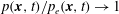 $p(\boldsymbol{x},t)/p_{e}(\boldsymbol{x},t)\rightarrow 1$
,
$p(\boldsymbol{x},t)/p_{e}(\boldsymbol{x},t)\rightarrow 1$
,
 $d(\boldsymbol{x},t)/d^{\ast }\rightarrow 0$
. For the case in which setting
$d(\boldsymbol{x},t)/d^{\ast }\rightarrow 0$
. For the case in which setting
 $l^{\ast }=l_{e}$
yields
$l^{\ast }=l_{e}$
yields
 $t_{e}\sim t^{\ast }$
, the characteristic parameters may be computed from (2.15). However, if setting
$t_{e}\sim t^{\ast }$
, the characteristic parameters may be computed from (2.15). However, if setting
 $l^{\ast }=l_{e}$
yields
$l^{\ast }=l_{e}$
yields
 $t_{e}/t^{\ast }\gg 1$
, the scaling is inconsistent and the viscous–elastic dynamics takes place on a length scale much greater than
$t_{e}/t^{\ast }\gg 1$
, the scaling is inconsistent and the viscous–elastic dynamics takes place on a length scale much greater than
 $l_{e}$
. In this case the characteristic time scale should be defined by the external actuation
$l_{e}$
. In this case the characteristic time scale should be defined by the external actuation
 $t^{\ast }=t_{e}$
instead of its length scale. The characteristic length scale of the viscous–elastic interaction can then be estimated from
$t^{\ast }=t_{e}$
instead of its length scale. The characteristic length scale of the viscous–elastic interaction can then be estimated from
 $l^{\ast }=(t_{e}h_{0}^{3}s/12{\it\mu})^{1/6}\gg l_{e}$
.
$l^{\ast }=(t_{e}h_{0}^{3}s/12{\it\mu})^{1/6}\gg l_{e}$
.
In addition, substituting (2.15) into (2.1) makes it possible to more clearly define the range of validity of the assumptions, yielding an equivalent definition of the Womersley number
 ${\it\varepsilon}_{1}^{5}{\it\rho}_{l}s/12{\it\mu}^{2}l^{\ast }\ll 1$
, and negligible plate inertia requirements
${\it\varepsilon}_{1}^{5}{\it\rho}_{l}s/12{\it\mu}^{2}l^{\ast }\ll 1$
, and negligible plate inertia requirements
 ${\it\varepsilon}_{1}^{6}{\it\rho}_{s}bs/144{\it\mu}^{2}l^{\ast }\ll 1$
. Utilizing order-of-magnitude analysis of the plate’s in-plane force equilibrium
${\it\varepsilon}_{1}^{6}{\it\rho}_{s}bs/144{\it\mu}^{2}l^{\ast }\ll 1$
. Utilizing order-of-magnitude analysis of the plate’s in-plane force equilibrium
 $n^{\ast }={\it\mu}u^{\ast }l^{\ast }/h_{0}$
, we obtain that the requirement for negligible membrane effects simplifies to
$n^{\ast }={\it\mu}u^{\ast }l^{\ast }/h_{0}$
, we obtain that the requirement for negligible membrane effects simplifies to
 ${\it\varepsilon}_{2}{\it\varepsilon}_{1}^{2}\ll 1$
. Therefore, the requirements of shallow geometry
${\it\varepsilon}_{2}{\it\varepsilon}_{1}^{2}\ll 1$
. Therefore, the requirements of shallow geometry
 ${\it\varepsilon}_{1}=h_{0}/l^{\ast }$
and small deformation to viscous film height ratio
${\it\varepsilon}_{1}=h_{0}/l^{\ast }$
and small deformation to viscous film height ratio
 ${\it\varepsilon}_{2}=d^{\ast }/h_{0}$
are sufficient in order to neglect membrane effects.
${\it\varepsilon}_{2}=d^{\ast }/h_{0}$
are sufficient in order to neglect membrane effects.
In the following sections we examine external pressures modelled as the Dirac delta function in time. The Dirac delta function represents an external pressure field that satisfies
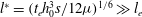
 $l_{e}/l^{\ast }\ll 1$
and
$l_{e}/l^{\ast }\ll 1$
and
 $t_{e}/t^{\ast }\ll 1$
. In this case we may choose arbitrarily
$t_{e}/t^{\ast }\ll 1$
. In this case we may choose arbitrarily
 $t^{\ast }$
or
$t^{\ast }$
or
 $l^{\ast }$
of interest, where we effectively only examine dynamics after the end of the external application of pressure. Due to the self-similar nature of the problem, the demand on order of magnitude smaller length-scale
$l^{\ast }$
of interest, where we effectively only examine dynamics after the end of the external application of pressure. Due to the self-similar nature of the problem, the demand on order of magnitude smaller length-scale
 $l_{e}/l^{\ast }\ll 1$
may be translated into additional demand on the time scale
$l_{e}/l^{\ast }\ll 1$
may be translated into additional demand on the time scale
 $t_{e}/t^{\ast }\ll 1$
. Thus, any external pressure distributed over a length scale of
$t_{e}/t^{\ast }\ll 1$
. Thus, any external pressure distributed over a length scale of
 $l_{e}$
may be modelled as the Dirac delta function for sufficiently large
$l_{e}$
may be modelled as the Dirac delta function for sufficiently large
 $t^{\ast }\gg 12{\it\mu}l_{e}^{6}/h_{0}^{3}~\text{s}$
. The validity of the assumptions (2.1) during the pressure application period should be examined with regard to
$t^{\ast }\gg 12{\it\mu}l_{e}^{6}/h_{0}^{3}~\text{s}$
. The validity of the assumptions (2.1) during the pressure application period should be examined with regard to
 $t_{e}$
and
$t_{e}$
and
 $l_{e}$
, representing dynamics during the pressure application, not the arbitrarily chosen
$l_{e}$
, representing dynamics during the pressure application, not the arbitrarily chosen
 $t^{\ast }$
and
$t^{\ast }$
and
 $l^{\ast }$
time and length scales.
$l^{\ast }$
time and length scales.
3 Green’s functions and self-similarity
The Green’s function of (2.13) and (2.14) is given by Satsanit & Kananthai (Reference Satsanit and Kananthai2009) as
 $$\begin{eqnarray}G={\displaystyle \frac{1}{4{\rm\pi}^{2}}}\int _{\mathbb{R}^{2}}\text{e}^{-(T-\bar{T})|{\bf\lambda}|^{6}+\text{i}{\bf\lambda}\boldsymbol{\cdot }(\boldsymbol{X}-\bar{\boldsymbol{X}})}\,\text{d}{\bf\lambda},\quad T>\bar{T},\end{eqnarray}$$
where
 $\bar{\boldsymbol{X}}$
and
$\bar{\boldsymbol{X}}$
and
 $\bar{T}$
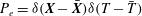
are the location and time of the delta function, respectively. Equation (3.1) represents the solution for the evolution of the pressure for external pressure,
$\bar{T}$
are the location and time of the delta function, respectively. Equation (3.1) represents the solution for the evolution of the pressure for external pressure,
 $\partial P_{e}/\partial T={\it\delta}(T-\bar{T}){\it\delta}(\boldsymbol{X}-\bar{\boldsymbol{X}})$
, and thus
$\partial P_{e}/\partial T={\it\delta}(T-\bar{T}){\it\delta}(\boldsymbol{X}-\bar{\boldsymbol{X}})$
, and thus
 $P_{e}={\it\theta}(T-\bar{T}){\it\delta}(\boldsymbol{X}-\bar{\boldsymbol{X}})+C_{1}(\boldsymbol{X})$
. Similarly, equation (3.1) represents the solution for the evolution equation of the deformation (2.13) for
$P_{e}={\it\theta}(T-\bar{T}){\it\delta}(\boldsymbol{X}-\bar{\boldsymbol{X}})+C_{1}(\boldsymbol{X})$
. Similarly, equation (3.1) represents the solution for the evolution equation of the deformation (2.13) for
 $\partial ^{2}P_{e}/\partial X^{2}={\it\delta}(T-\bar{T}){\it\delta}(\boldsymbol{X}-\bar{\boldsymbol{X}})$
and thus
$\partial ^{2}P_{e}/\partial X^{2}={\it\delta}(T-\bar{T}){\it\delta}(\boldsymbol{X}-\bar{\boldsymbol{X}})$
and thus
 $P_{e}={\it\delta}(T-\bar{T}){\it\theta}(\boldsymbol{X}-\bar{\boldsymbol{X}})\boldsymbol{X}+X\cdot C_{1}(T)+C_{2}(T)$
. We note that external pressures of the form
$P_{e}={\it\delta}(T-\bar{T}){\it\theta}(\boldsymbol{X}-\bar{\boldsymbol{X}})\boldsymbol{X}+X\cdot C_{1}(T)+C_{2}(T)$
. We note that external pressures of the form
 $P_{e}=X\cdot C_{1}(T)+C_{2}(T)$
do not create deformation of the plate.
$P_{e}=X\cdot C_{1}(T)+C_{2}(T)$
do not create deformation of the plate.
Equation (3.1) may be interpreted as the inverse Fourier transform, where the argument of transformation is
 $\text{e}^{-(T-\bar{T})|{\bf\lambda}|^{6}}$
. Furthermore, the radial symmetry of the argument enables representation of (3.1) by the inverse Hankel transform
$\text{e}^{-(T-\bar{T})|{\bf\lambda}|^{6}}$
. Furthermore, the radial symmetry of the argument enables representation of (3.1) by the inverse Hankel transform
 $$\begin{eqnarray}G={\displaystyle \frac{1}{2{\rm\pi}}}\int _{0}^{\infty }\text{e}^{-(T-\bar{T}){\it\rho}^{6}}J_{0}({\it\rho}|\boldsymbol{X}-\bar{\boldsymbol{X}}|){\it\rho}\,\text{d}{\it\rho}.\end{eqnarray}$$
Expressing the Bessel function in a series form, and integrating each element according to
 $$\begin{eqnarray}\int _{0}^{\infty }l^{m}\text{e}^{-{\it\beta}l^{n}}\text{d}l={\displaystyle \frac{{\it\Gamma}({\it\gamma})}{n{\it\beta}^{{\it\gamma}}}},\quad {\it\gamma}={\displaystyle \frac{m+1}{n}},\end{eqnarray}$$
where
 ${\it\Gamma}({\it\gamma})$
is the gamma function, yields a self-similar expression
${\it\Gamma}({\it\gamma})$
is the gamma function, yields a self-similar expression
 $$\begin{eqnarray}G={\displaystyle \frac{{\it\Psi}({\it\eta})}{(T-\bar{T})^{1/3}}},\quad {\it\eta}={\displaystyle \frac{|\boldsymbol{X}-\bar{\boldsymbol{X}}|}{6(T-\bar{T})^{1/6}}},\end{eqnarray}$$
where
 $$\begin{eqnarray}{\it\Psi}({\it\eta})={\displaystyle \frac{1}{12{\rm\pi}}}\mathop{\sum }_{m=0}^{\infty }{\displaystyle \frac{3^{2m}{\it\Gamma}(1+m/3)(-1)^{m}}{{\it\Gamma}(m+1)^{2}}}{\it\eta}^{2m}.\end{eqnarray}$$
We decompose the series into three separate series
 $$\begin{eqnarray}\mathop{\sum }_{k=0}^{\infty }a_{m}{\it\eta}^{k}=\mathop{\sum }_{k=0}^{\infty }a_{3k}{\it\eta}^{3k}+\mathop{\sum }_{k=0}^{\infty }a_{3k+1}{\it\eta}^{3k+1}+\mathop{\sum }_{k=0}^{\infty }a_{km+2}{\it\eta}^{3k+2}\end{eqnarray}$$
thus yielding a closed-form expression in terms of generalized hyper-geometric functions (Slater Reference Slater1966; Bailey Reference Bailey1972)
 $$\begin{eqnarray}\displaystyle {\it\Psi}({\it\eta}) & = & \displaystyle {\displaystyle \frac{1}{12{\rm\pi}}}\bigg[{\it\Gamma}\left({\displaystyle \frac{1}{3}}\right)\,_{0}F_{4}\left(;{\displaystyle \frac{1}{3}},{\displaystyle \frac{2}{3}},{\displaystyle \frac{2}{3}},1;-{\it\eta}^{6}\right)\nonumber\\ \displaystyle & & \displaystyle -9{\it\eta}^{2}{\it\Gamma}\left({\displaystyle \frac{2}{3}}\right)\,_{0}F_{4}\left(;{\displaystyle \frac{2}{3}},1,{\displaystyle \frac{4}{3}},{\displaystyle \frac{4}{3}};-{\it\eta}^{6}\right)+{\displaystyle \frac{81}{4}}{\it\eta}^{4}\,_{0}F_{4}\left(;{\displaystyle \frac{4}{3}},{\displaystyle \frac{4}{3}},{\displaystyle \frac{5}{3}},{\displaystyle \frac{5}{3}};-{\it\eta}^{6}\right)\bigg].\nonumber\\ \displaystyle & & \displaystyle\end{eqnarray}$$
While the function presented in (3.7) can be used by convolution to obtain a general solution, more insight may be obtained from a solution for the case of
 $P_{e}={\it\delta}(\boldsymbol{X}-\bar{\boldsymbol{X}}){\it\delta}(T-\bar{T})$
. This may be achieved without convolution by applying the Laplacian operator in terms of
$P_{e}={\it\delta}(\boldsymbol{X}-\bar{\boldsymbol{X}}){\it\delta}(T-\bar{T})$
. This may be achieved without convolution by applying the Laplacian operator in terms of
 $\bar{\boldsymbol{X}}$
(i.e.
$\bar{\boldsymbol{X}}$
(i.e.
 ${\it\Delta}_{\bar{\boldsymbol{X}}}$
) on the equation defining the Green’s function. Linearity of the equation, and the relation
${\it\Delta}_{\bar{\boldsymbol{X}}}$
) on the equation defining the Green’s function. Linearity of the equation, and the relation
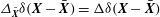 ${\it\Delta}_{\bar{\boldsymbol{X}}}{\it\delta}(\boldsymbol{X}-\bar{\boldsymbol{X}})={\rm\Delta}{\it\delta}(\boldsymbol{X}-\bar{\boldsymbol{X}})$
, yields
${\it\Delta}_{\bar{\boldsymbol{X}}}{\it\delta}(\boldsymbol{X}-\bar{\boldsymbol{X}})={\rm\Delta}{\it\delta}(\boldsymbol{X}-\bar{\boldsymbol{X}})$
, yields
 $$\begin{eqnarray}\left({\displaystyle \frac{\partial }{\partial T}}-{\rm\nabla}^{6}\right){\it\Delta}_{\bar{\boldsymbol{X}}}G={\rm\Delta}{\it\delta}(\boldsymbol{X}-\bar{\boldsymbol{X}}){\it\delta}(T-\bar{T}).\end{eqnarray}$$
Thus, the deformation field due to a unit impulse is
 $$\begin{eqnarray}G_{d}={\it\Delta}_{\bar{\boldsymbol{X}}}G={\displaystyle \frac{{\it\Psi}_{d}({\it\eta})}{(T-\bar{T})^{2/3}}},\end{eqnarray}$$
where
 $$\begin{eqnarray}\displaystyle {\it\Psi}_{d} & = & \displaystyle -{\displaystyle \frac{1}{48{\rm\pi}}}\bigg[4{\it\Gamma}\left({\displaystyle \frac{2}{3}}\right)\,_{0}F_{4}\left(;{\displaystyle \frac{1}{3}},{\displaystyle \frac{1}{3}},{\displaystyle \frac{2}{3}},1;-{\it\eta}^{6}\right)\nonumber\\ \displaystyle & & \displaystyle +\,27{\it\eta}^{4}{\it\Gamma}\left({\displaystyle \frac{1}{3}}\right)\,_{0}F_{4}\left(;1,{\displaystyle \frac{4}{3}},{\displaystyle \frac{5}{3}},{\displaystyle \frac{5}{3}};-{\it\eta}^{6}\right)\nonumber\\ \displaystyle & & \displaystyle -\,36{\it\eta}^{2}\,_{0}F_{4}\left(;{\displaystyle \frac{2}{3}},{\displaystyle \frac{2}{3}},{\displaystyle \frac{4}{3}},{\displaystyle \frac{4}{3}};-{\it\eta}^{6}\right)\bigg].\end{eqnarray}$$
A similar approach may be used to obtain the pressure field due to a unit impulse, yielding
 $$\begin{eqnarray}G_{p}=-{\displaystyle \frac{\partial G}{\partial \bar{T}}}={\displaystyle \frac{{\it\Psi}_{p}({\it\eta})}{(T-\bar{T})^{4/3}}},\end{eqnarray}$$
where
 $$\begin{eqnarray}\displaystyle {\it\Psi}_{p} & = & \displaystyle -{\displaystyle \frac{1}{36{\rm\pi}}}\left[{\it\Gamma}\left({\displaystyle \frac{1}{3}}\right)\,_{1}F_{5}\left({\displaystyle \frac{4}{3}};{\displaystyle \frac{1}{3}},{\displaystyle \frac{1}{3}},{\displaystyle \frac{2}{3}},{\displaystyle \frac{2}{3}},1;-{\it\eta}^{6}\right)\right.\nonumber\\ \displaystyle & & \displaystyle +\,{\displaystyle \frac{243}{4}}{\it\eta}^{4}\,_{1}F_{5}\left(2;1,{\displaystyle \frac{4}{3}},{\displaystyle \frac{4}{3}},{\displaystyle \frac{5}{3}},{\displaystyle \frac{5}{3}};-{\it\eta}^{6}\right)\nonumber\\ \displaystyle & & \displaystyle \left.-\,18{\it\eta}^{2}{\it\Gamma}\left({\displaystyle \frac{2}{3}}\right)\,_{1}F_{5}\left({\displaystyle \frac{5}{3}};{\displaystyle \frac{2}{3}},{\displaystyle \frac{2}{3}},1,{\displaystyle \frac{4}{3}},{\displaystyle \frac{4}{3}};-{\it\eta}^{6}\right)\right].\end{eqnarray}$$
 $G_{p}$
,
$G_{p}$
,
 $G_{d}$
thus give more direct insight regarding the response to external forces and may be used to convolve
$G_{d}$
thus give more direct insight regarding the response to external forces and may be used to convolve
 $P_{e}$
directly for general solutions, similarly to a regular Green’s function. We note that the characteristic liquid pressure
$P_{e}$
directly for general solutions, similarly to a regular Green’s function. We note that the characteristic liquid pressure
 $p^{\ast }=j_{e}/l^{\ast 2}t^{\ast }$
, where
$p^{\ast }=j_{e}/l^{\ast 2}t^{\ast }$
, where
 $j_{e}$
is the magnitude of impulse.
$j_{e}$
is the magnitude of impulse.
Without loss of generality, we hereafter assign
 $\bar{T}=0$
. From
$\bar{T}=0$
. From
 ${\it\eta}$
, the radial speed of the signal propagation is obtained as
${\it\eta}$
, the radial speed of the signal propagation is obtained as
 ${\it\eta}_{ref}T^{-5/6}$
, where
${\it\eta}_{ref}T^{-5/6}$
, where
 ${\it\eta}_{ref}$
is a reference state. Utilizing equations (2.10) and (2.9) together with
${\it\eta}_{ref}$
is a reference state. Utilizing equations (2.10) and (2.9) together with
 $G_{p}=T^{-4/3}{\it\Psi}_{p}({\it\eta})$
we obtain the radial and transverse fluid speed
$G_{p}=T^{-4/3}{\it\Psi}_{p}({\it\eta})$
we obtain the radial and transverse fluid speed
 $G_{u}=T^{-3/2}{\it\Psi}_{u}({\it\eta})$
,
$G_{u}=T^{-3/2}{\it\Psi}_{u}({\it\eta})$
,
 $G_{w}=T^{-5/3}{\it\Psi}_{w}({\it\eta})$
, respectively. Substituting
$G_{w}=T^{-5/3}{\it\Psi}_{w}({\it\eta})$
, respectively. Substituting
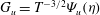
 $G_{d}=T^{-2/3}{\it\Psi}_{d}({\it\eta})$
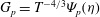
into the plate’s constitutive equations (Timoshenko & Woinowsky-Krieger Reference Timoshenko and Woinowsky-Krieger1959; Reddy Reference Reddy2006) we obtain the bending moment
$G_{d}=T^{-2/3}{\it\Psi}_{d}({\it\eta})$
into the plate’s constitutive equations (Timoshenko & Woinowsky-Krieger Reference Timoshenko and Woinowsky-Krieger1959; Reddy Reference Reddy2006) we obtain the bending moment
 $G_{m}=T^{-1}{\it\Psi}_{m}({\it\eta})$
and shear force
$G_{m}=T^{-1}{\it\Psi}_{m}({\it\eta})$
and shear force
 $G_{q}=T^{-7/6}{\it\Psi}_{q}({\it\eta})$
.
$G_{q}=T^{-7/6}{\it\Psi}_{q}({\it\eta})$
.
 ${\it\Psi}_{p}$
,
${\it\Psi}_{p}$
,
 ${\it\Psi}_{u}$
,
${\it\Psi}_{u}$
,
 ${\it\Psi}_{w}$
are presented in figure 2(a) (solid, dashed and dotted lines, respectively) and
${\it\Psi}_{w}$
are presented in figure 2(a) (solid, dashed and dotted lines, respectively) and
 ${\it\Psi}_{d}$
,
${\it\Psi}_{d}$
,
 ${\it\Psi}_{m}$
,
${\it\Psi}_{m}$
,
 ${\it\Psi}_{q}$
are presented in figure 2(b) (solid, dashed and dotted lines, respectively). All
${\it\Psi}_{q}$
are presented in figure 2(b) (solid, dashed and dotted lines, respectively). All
 ${\it\Psi}_{i}$
, (
${\it\Psi}_{i}$
, (
 $i=p,u,w,d,m,q$
) are similar decaying oscillating functions of
$i=p,u,w,d,m,q$
) are similar decaying oscillating functions of
 ${\it\eta}$
. However, a difference in the decay rate in time exists due to the different powers of
${\it\eta}$
. However, a difference in the decay rate in time exists due to the different powers of
 $T$
multiplying
$T$
multiplying
 ${\it\Psi}_{i}$
, where the slowest time decay is of the deformation, scaling as
${\it\Psi}_{i}$
, where the slowest time decay is of the deformation, scaling as
 $T^{-2/3}$
.
$T^{-2/3}$
.

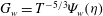
Figure 2. The similarity shape function versus
 ${\it\eta}$
: (a) pressure (solid), radial liquid velocity (dashed), transverse liquid velocity (dotted); (b) deformation (solid), bending moment (dashed) and transverse shear force (dotted).
${\it\eta}$
: (a) pressure (solid), radial liquid velocity (dashed), transverse liquid velocity (dotted); (b) deformation (solid), bending moment (dashed) and transverse shear force (dotted).

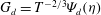
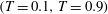
Figure 3. Dynamics during and after application of a temporally uniform external force applied at
 $\boldsymbol{X}=\bar{\boldsymbol{X}}$
: (a,b) show the pressure and deformation during
$\boldsymbol{X}=\bar{\boldsymbol{X}}$
: (a,b) show the pressure and deformation during
 $(T=0.1,T=0.9)$
and after
$(T=0.1,T=0.9)$
and after
 $(T=1.1,T=2)$
application of the external pressure, respectively, where
$(T=1.1,T=2)$
application of the external pressure, respectively, where
 $T_{e}=1$
. The inserts in (a,b) present the time evolution of the pressure and deformation at the impact locus, respectively.
$T_{e}=1$
. The inserts in (a,b) present the time evolution of the pressure and deformation at the impact locus, respectively.
4 Impact mitigation and response dynamics to spatially and temporally distributed external forces
The functions (3.4), (3.9) and (3.11) can now be used to examine the fluid pressure field and plate deformation field created during and after application of spatially and temporally distributed external forces. For a temporally uniform external force applied at
 $\boldsymbol{X}=\bar{\boldsymbol{X}}$
over a finite time interval, defined as
$\boldsymbol{X}=\bar{\boldsymbol{X}}$
over a finite time interval, defined as
 $$\begin{eqnarray}P_{e}={\displaystyle \frac{1}{T_{e}}}{\it\delta}(\boldsymbol{X}-\bar{\boldsymbol{X}},T)[{\it\theta}(T)-{\it\theta}(T-T_{e})],\end{eqnarray}$$
where
 ${\it\theta}$
is the Heaviside function and
${\it\theta}$
is the Heaviside function and
 $T_{e}$
is the instant of release, the pressure field is immediately obtained from (3.4) as
$T_{e}$
is the instant of release, the pressure field is immediately obtained from (3.4) as
 $$\begin{eqnarray}P={\displaystyle \frac{1}{T_{e}}}\left\{\begin{array}{@{}ll@{}}G({\it\eta},T),\quad & T<T_{e}\\ G(T)-G(T-T_{e}),\quad & T>T_{e}.\end{array}\right.\end{eqnarray}$$
Similarly, substituting (4.2) into (2.12) and integrating with respect to
 $T$
, yields the deformation of the elastic plate. Figure 3(a) presents the fluid pressure field at two instants during (
$T$
, yields the deformation of the elastic plate. Figure 3(a) presents the fluid pressure field at two instants during (
 $T=0.1,0.9$
) and after (
$T=0.1,0.9$
) and after (
 $T=1.1,2$
) the application of external force of the form of (4.1), where
$T=1.1,2$
) the application of external force of the form of (4.1), where
 $T_{e}=1$
. During the application (
$T_{e}=1$
. During the application (
 $T<T_{e}$
), the pressure in the impact locus decays with time and acts to resist the temporally constant external force. After the application period (
$T<T_{e}$
), the pressure in the impact locus decays with time and acts to resist the temporally constant external force. After the application period (
 $T>T_{e}$
), the pressure at the locus instantaneously changes sign, now working to resist the plate’s relaxation and increases with time. The insert in figure 3(a) focuses on pressure at the locus of application of the external force, given by
$T>T_{e}$
), the pressure at the locus instantaneously changes sign, now working to resist the plate’s relaxation and increases with time. The insert in figure 3(a) focuses on pressure at the locus of application of the external force, given by
 $$\begin{eqnarray}P(\boldsymbol{X}=\bar{\boldsymbol{X}})={\displaystyle \frac{1}{T_{e}}}\left\{\begin{array}{@{}ll@{}}{\displaystyle \frac{{\it\Gamma}\left({\displaystyle \frac{1}{3}}\right)}{12{\rm\pi}}}{\displaystyle \frac{1}{T^{1/3}}},\quad & T<T_{e}\\ {\displaystyle \frac{{\it\Gamma}\left({\displaystyle \frac{1}{3}}\right)}{12{\rm\pi}}}\left({\displaystyle \frac{1}{T^{1/3}}}-{\displaystyle \frac{1}{(T-T_{e}){\displaystyle \frac{1}{3}}}}\right),\quad & T>T_{e}.\end{array}\right.\end{eqnarray}$$
From (4.3), the rate of decay during application is
 ${\sim}T^{-1/3}$
, and a discontinuity in pressure occurs at the instant of release (
${\sim}T^{-1/3}$
, and a discontinuity in pressure occurs at the instant of release (
 $T=T_{e}$
) of the external force.
$T=T_{e}$
) of the external force.
Figure 3(b) presents the deformation field created in the elastic plate. While the deformation near the impact locus is negative, there is a region of significant positive deformation adjacent to the minima at the locus. An infinite number of maximum points of the deformations are expected from (3.9). However, all other maximum points are small in magnitude compared with the deformation near the locus. The maxima of this primary positive deformation region propagate radially both during and after the application of the external pressure field. The insert in figure 3(b) focuses on deformation at the locus, given by
 $$\begin{eqnarray}D(\boldsymbol{X}=\bar{\boldsymbol{X}})={\displaystyle \frac{1}{T_{e}}}\left\{\begin{array}{@{}ll@{}}{\displaystyle \frac{{\it\Gamma}\left(-{\displaystyle \frac{1}{3}}\right)}{6}}T^{1/3},\quad & T<T_{e}\\ {\displaystyle \frac{{\it\Gamma}\left(-{\displaystyle \frac{1}{3}}\right)}{6}}\left(T^{1/3}-\left(T-T_{e}\right)^{1/3}\right),\quad & T>T_{e}.\end{array}\right.\end{eqnarray}$$
From (4.4), the deformation during force application is shown to increase as a power of
 $T^{1/3}$
, and have a discontinuity in the rate of deformation at the moment of release of the external pressure (
$T^{1/3}$
, and have a discontinuity in the rate of deformation at the moment of release of the external pressure (
 $T=T_{e}$
). This discontinuity may locally give rise to inertial effects which will invalidate assumptions (2.1) for
$T=T_{e}$
). This discontinuity may locally give rise to inertial effects which will invalidate assumptions (2.1) for
 $T\rightarrow T_{e}$
(see discussion at the end of § 2). Specifically, the solution will be valid only for time scales much greater than the inertial plate time scale
$T\rightarrow T_{e}$
(see discussion at the end of § 2). Specifically, the solution will be valid only for time scales much greater than the inertial plate time scale
 $\sqrt{{\it\rho}_{s}bl_{e}^{4}/s}$
, where
$\sqrt{{\it\rho}_{s}bl_{e}^{4}/s}$
, where
 $l_{e}$
is the finite actuation length scale. We note that the characteristic liquid pressure is defined as
$l_{e}$
is the finite actuation length scale. We note that the characteristic liquid pressure is defined as
 $p^{\ast }=f_{e}/l^{\ast 2}$
, where
$p^{\ast }=f_{e}/l^{\ast 2}$
, where
 $f_{e}$
is the magnitude of the external force.
$f_{e}$
is the magnitude of the external force.
We now turn to explore the relation between the externally applied pressure field and the fluidic pressure field in order to examine the impact mitigation properties of such configurations. This necessitates examination of finite external pressures, distributed both spatially and temporally. We initially focus on a suddenly applied external pressure, uniform in both space and time with a time period
 $T_{e,1}$
, a spatial radius
$T_{e,1}$
, a spatial radius
 $L_{e}$
and a constant total impulse of
$L_{e}$
and a constant total impulse of
 $1$
, given by
$1$
, given by
 $$\begin{eqnarray}P_{e,1}={\displaystyle \frac{1}{{\rm\pi}L_{e}^{2}T_{e,1}}}{\it\theta}(L_{e}-|\boldsymbol{X}|)[{\it\theta}(T)-{\it\theta}(T-T_{e,1})].\end{eqnarray}$$
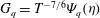
Convolving (3.11) with (4.5), the pressure ratio between the externally applied pressure and the fluidic pressure at the centre
 $\boldsymbol{X}=0$
can be estimated for
$\boldsymbol{X}=0$
can be estimated for
 $T\leqslant T_{e,1}$
as
$T\leqslant T_{e,1}$
as
 $$\begin{eqnarray}\displaystyle {\displaystyle \frac{P(\boldsymbol{X}=0)}{P_{e,1}}} & = & \displaystyle 1-\,_{0}F_{4}\left(;{\displaystyle \frac{1}{3}},{\displaystyle \frac{1}{3}},{\displaystyle \frac{2}{3}},{\displaystyle \frac{2}{3}};-{\it\eta}_{L_{e}}^{6}\right)\nonumber\\ \displaystyle & & \displaystyle -\,{\displaystyle \frac{27}{2}}{\it\eta}_{L_{e}}^{4}{\it\Gamma}\left({\displaystyle \frac{2}{3}}\right)\,_{0}F_{4}\left(;1,{\displaystyle \frac{4}{3}},{\displaystyle \frac{4}{3}},{\displaystyle \frac{5}{3}};-{\it\eta}_{L_{e}}^{6}\right)\nonumber\\ \displaystyle & & \displaystyle +\,3{\it\eta}_{L_{e}}^{2}{\it\Gamma}\left({\displaystyle \frac{1}{3}}\right)\,_{0}F_{4}\left(;{\displaystyle \frac{2}{3}},{\displaystyle \frac{2}{3}},1,{\displaystyle \frac{4}{3}};-{\it\eta}_{L_{e}}^{6}\right),\end{eqnarray}$$
where
 ${\it\eta}_{L_{e}}=L_{e}/6T^{1/6}$
. Equation (4.6) is presented in figure 4 (solid line). Three distinct periods are evident.
${\it\eta}_{L_{e}}=L_{e}/6T^{1/6}$
. Equation (4.6) is presented in figure 4 (solid line). Three distinct periods are evident.
-
(i) An initial period of the impact,
 $2.5\lesssim {\it\eta}_{L_{e}}<\infty$
, where the fluidic pressure closely follows the external pressure.
$2.5\lesssim {\it\eta}_{L_{e}}<\infty$
, where the fluidic pressure closely follows the external pressure. -
(ii) The interval,
$0.5\lesssim {\it\eta}_{L_{e}}\lesssim 2.5$
, shows small oscillations of the pressure ratio going from mitigation to amplification and vice versa. -
(iii) The period
$0\leqslant {\it\eta}_{L_{e}}\lesssim 0.5$
where mitigation occurs and grows with time.


However, since at the application of the suddenly applied external pressure,
 $T=0^{+}$
and thus, as
$T=0^{+}$
and thus, as
 ${\it\eta}_{L_{e}}\rightarrow \infty$
where
${\it\eta}_{L_{e}}\rightarrow \infty$
where
 $P(\boldsymbol{X}=0)\rightarrow P_{e,1}$
, no mitigation can be achieved from external pressures where the rise time is an order of magnitude smaller than the viscous–elastic time scale. Furthermore, in such configurations viscous–elastic interaction may amplify fluidic pressure to
$P(\boldsymbol{X}=0)\rightarrow P_{e,1}$
, no mitigation can be achieved from external pressures where the rise time is an order of magnitude smaller than the viscous–elastic time scale. Furthermore, in such configurations viscous–elastic interaction may amplify fluidic pressure to
 ${\sim}1.3P_{e,1}$
.
${\sim}1.3P_{e,1}$
.

Figure 4. (a) The liquid pressure at
 $\boldsymbol{X}=0$
divided by the external pressure during the application period versus
$\boldsymbol{X}=0$
divided by the external pressure during the application period versus
 ${\it\eta}_{L_{e}}=L_{e}/6T^{1/6}$
. The solid line denotes the ratio of pressures as a result of an external pressure rapidly applied at
${\it\eta}_{L_{e}}=L_{e}/6T^{1/6}$
. The solid line denotes the ratio of pressures as a result of an external pressure rapidly applied at
 $T=0$
and constant throughout the application period. The dashed line denotes the ratio of pressures as a result of an external pressure linearly increasing with time. Both external pressures are distributed evenly on a disk of radius
$T=0$
and constant throughout the application period. The dashed line denotes the ratio of pressures as a result of an external pressure linearly increasing with time. Both external pressures are distributed evenly on a disk of radius
 $L_{e}$
. The insert shows a schematic illustration of the evolution of the external pressures in time for both cases. (b) Ratio of the liquid pressure at the centre of impact to the external pressure,
$L_{e}$
. The insert shows a schematic illustration of the evolution of the external pressures in time for both cases. (b) Ratio of the liquid pressure at the centre of impact to the external pressure,
 $P_{e,2}$
, at the moment of maximal external pressure,
$P_{e,2}$
, at the moment of maximal external pressure,
 $T=T_{e,2}$
. External radii
$T=T_{e,2}$
. External radii
 $L_{e}=0.1$
,
$L_{e}=0.1$
,
 $0.3$
,
$0.3$
,
 $0.6$
,
$0.6$
,
 $1.2$
,
$1.2$
,
 $2.4$
,
$2.4$
,
 $4.8$
correspond to orange, brown, green, blue, purple and red lines, respectively. The insert shows schematically the evolution of the external pressure in time.
$4.8$
correspond to orange, brown, green, blue, purple and red lines, respectively. The insert shows schematically the evolution of the external pressure in time.
Next, we turn to examine time-varying external pressures with a rise time of the order of magnitude of the viscous–elastic time scale. We model an external pressure field, evenly distributed on a disk of radius
 $L_{e}$
, linearly increasing in magnitude with respect to time until
$L_{e}$
, linearly increasing in magnitude with respect to time until
 $T_{e,2}$
and then decreasing linearly until vanishing at
$T_{e,2}$
and then decreasing linearly until vanishing at
 $2T_{e,2}$
(see insert in figure 4
b). The total impulse is
$2T_{e,2}$
(see insert in figure 4
b). The total impulse is
 $1$
, and
$1$
, and
 $P_{e,2}$
is thus given by
$P_{e,2}$
is thus given by
 $$\begin{eqnarray}P_{e,2}={\displaystyle \frac{{\it\theta}(L_{e}-|\boldsymbol{X}|)}{{\rm\pi}L_{e}^{2}T_{e,2}^{2}}}[T{\it\theta}(T)-2(T-T_{e,2}){\it\theta}(T-T_{e,2})+(T-2T_{e,2}){\it\theta}(T-2T_{e,2})].\end{eqnarray}$$
Convolving (3.11) with (4.7), denoting
 ${\it\eta}_{L_{e}}=L_{e}/6T^{1/6}$
and dividing by
${\it\eta}_{L_{e}}=L_{e}/6T^{1/6}$
and dividing by
 $P_{e,2}$
yields the ratio of pressures at the centre for
$P_{e,2}$
yields the ratio of pressures at the centre for
 $T\leqslant T_{e,2}$
 $$\begin{eqnarray}{\displaystyle \frac{P(\boldsymbol{X}=0,T)}{P_{e,2}(T)}}={\it\eta}_{L_{e}}^{6}G_{2,7}^{4,1}\left({\it\eta}_{L_{e}}^{6}|\begin{array}{@{}c@{}}0,1\\ -{\displaystyle \frac{2}{3}},-{\displaystyle \frac{1}{3}},0,0,-1,-{\displaystyle \frac{2}{3}},-{\displaystyle \frac{1}{3}}\\ \end{array}\right),\end{eqnarray}$$
where
 $G_{2,7}^{4,1}$
is the Meijer
$G_{2,7}^{4,1}$
is the Meijer
 $G$
-function (Bateman & Erdelyi Reference Bateman and Erdelyi1953; Luke Reference Luke1969). The result is shown in figure 4(a) with respect to similarity variable
$G$
-function (Bateman & Erdelyi Reference Bateman and Erdelyi1953; Luke Reference Luke1969). The result is shown in figure 4(a) with respect to similarity variable
 ${\it\eta}_{L_{e}}$
(dashed line) and with respect to the time when maximal external pressure is reached (i.e.
${\it\eta}_{L_{e}}$
(dashed line) and with respect to the time when maximal external pressure is reached (i.e.
 $T_{e,2}$
) in figure 4(b). From figure 4, it is evident that for any width of external pressure
$T_{e,2}$
) in figure 4(b). From figure 4, it is evident that for any width of external pressure
 $L_{e}$
, mitigation may be achieved if the application time is sufficiently long
$L_{e}$
, mitigation may be achieved if the application time is sufficiently long
 $$\begin{eqnarray}{\it\eta}_{L_{e}}(T=T_{e,2})={\displaystyle \frac{L_{e}}{6T_{e,2}^{6}}}\lesssim {\displaystyle \frac{1}{2}}.\end{eqnarray}$$
Specifically, for the case of
 $L_{e}=0.1$
, mitigation of more than
$L_{e}=0.1$
, mitigation of more than
 $90\,\%$
is achieved for external pressures applied over the period of
$90\,\%$
is achieved for external pressures applied over the period of
 $T_{e,2}=10^{-3}$
or longer.
$T_{e,2}=10^{-3}$
or longer.

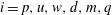
Figure 5. (a) Schematic illustration of the experimental set-up consisting of a thin elastic plate floating over a liquid film. At the centre of the plate a linear actuator deforms the plate and the force applied is measured by a load cell connected to the actuator. The deformation profile is sampled by a laser profilometer. (b) Experimental and theoretical deformation
 $d$
versus
$d$
versus
 $r$
during the application of the external force
$r$
during the application of the external force
 $f_{e}$
. Theoretical deformation profiles are obtained by convolution of
$f_{e}$
. Theoretical deformation profiles are obtained by convolution of
 $g_{d}$
with
$g_{d}$
with
 $f_{e}$
and are presented by smooth lines (red, blue and yellow, corresponding to
$f_{e}$
and are presented by smooth lines (red, blue and yellow, corresponding to
 $t=0.4~\text{s}$
,
$t=0.4~\text{s}$
,
 $t=0.6~\text{s}$
and
$t=0.6~\text{s}$
and
 $t=0.8~\text{s}$
, respectively). Circular markers (red, blue and yellow corresponding to
$t=0.8~\text{s}$
, respectively). Circular markers (red, blue and yellow corresponding to
 $t=0.4~\text{s}$
,
$t=0.4~\text{s}$
,
 $t=0.6~\text{s}$
and
$t=0.6~\text{s}$
and
 $t=0.8~\text{s}$
, respectively) present the mean value of the experimental data acquired by the laser profilometer. The insert shows the mean value of load cell measurements
$t=0.8~\text{s}$
, respectively) present the mean value of the experimental data acquired by the laser profilometer. The insert shows the mean value of load cell measurements
 $f_{e}$
versus time
$f_{e}$
versus time
 $t$
. Error bars depict one standard deviation.
$t$
. Error bars depict one standard deviation.
5 Experimental verification
Experiments were conducted to illustrate and verify some of the theoretical results of § 3. The experimental set-up (see figure 5
a) consists of a polyurethane rubber plate (Econ®-60 urethane rubber) floating over a thin silicon-oil film (Xiameter® PMX-200 silicone fluid). The centre of the plate is deformed at a constant velocity of
 $10~\text{mm}~\text{s}^{-1}$
due to application of a spherical indenter with radius of 5 mm. The indenter is connected to a linear actuator (Thorlabs™ DRV013) and a load cell measuring the force applied on the elastic plate. The radial deformation profile created during force application is sampled by a laser profilometer (MicroEpsilon™ ScanControl 2650-100).
$10~\text{mm}~\text{s}^{-1}$
due to application of a spherical indenter with radius of 5 mm. The indenter is connected to a linear actuator (Thorlabs™ DRV013) and a load cell measuring the force applied on the elastic plate. The radial deformation profile created during force application is sampled by a laser profilometer (MicroEpsilon™ ScanControl 2650-100).
Relevant physical properties of the configuration are the elastic plate thickness
 $b=5.5~\text{mm}$
, elastic plate diameter
$b=5.5~\text{mm}$
, elastic plate diameter
 $238~\text{mm}$
, plate bending resistance
$238~\text{mm}$
, plate bending resistance
 $s=0.01~\text{Pa}~\text{m}^{3}$
, plate material density
$s=0.01~\text{Pa}~\text{m}^{3}$
, plate material density
 ${\it\rho}_{s}=954~\text{Kg}~\text{m}^{-3}$
, liquid viscosity
${\it\rho}_{s}=954~\text{Kg}~\text{m}^{-3}$
, liquid viscosity
 ${\it\mu}=60~\text{Pa}~\text{s}$
, liquid density
${\it\mu}=60~\text{Pa}~\text{s}$
, liquid density
 ${\it\rho}_{l}=987~\text{Kg}~\text{m}^{-3}$
and initial gap
${\it\rho}_{l}=987~\text{Kg}~\text{m}^{-3}$
and initial gap
 $h_{0}=6~\text{mm}$
. Figure 5(b) shows the mean value of four experimental measurements (red, blue and yellow circles, corresponding to
$h_{0}=6~\text{mm}$
. Figure 5(b) shows the mean value of four experimental measurements (red, blue and yellow circles, corresponding to
 $t=0.4~\text{s}$
,
$t=0.4~\text{s}$
,
 $t=0.6~\text{s}$
and
$t=0.6~\text{s}$
and
 $t=0.8~\text{s}$
, respectively) and theoretical predictions (red, blue and yellow lines, corresponding to
$t=0.8~\text{s}$
, respectively) and theoretical predictions (red, blue and yellow lines, corresponding to
 $t=0.4~\text{s}$
,
$t=0.4~\text{s}$
,
 $t=0.6~\text{s}$
and
$t=0.6~\text{s}$
and
 $t=0.8~\text{s}$
, respectively) versus the radial coordinate
$t=0.8~\text{s}$
, respectively) versus the radial coordinate
 $r$
. The insert in figure 5(b) shows the mean value of force measurements
$r$
. The insert in figure 5(b) shows the mean value of force measurements
 $f_{e}(N)$
, applied by the actuator on the centre of the plate versus time
$f_{e}(N)$
, applied by the actuator on the centre of the plate versus time
 $t(s)$
. Error bars indicate one standard deviation. The theoretical deformation is obtained by convolution of the external force measurements with (3.9) (see equation (A 9)). The radial location of the minimal radius measured by the laser profilometer was estimated by correlation to the analytic solution as
$t(s)$
. Error bars indicate one standard deviation. The theoretical deformation is obtained by convolution of the external force measurements with (3.9) (see equation (A 9)). The radial location of the minimal radius measured by the laser profilometer was estimated by correlation to the analytic solution as
 $r=20~\text{mm}$
. No other fitting parameters are used and good agreement between the analytical results and experimental data is evident.
$r=20~\text{mm}$
. No other fitting parameters are used and good agreement between the analytical results and experimental data is evident.
6 Concluding remarks
In this work we examine the dynamics of a liquid film enclosed between a rigid surface and an elastic plate, under the effect of time-varying external forces acting on the plate. The presence of a thin viscous film between the upper plate and the lower surface is shown to distribute localized external forces, where the characteristic speed of fluid pressure propagation is
 $O(h_{0}^{3}s/12{\it\mu}l_{e}^{5})$
(for viscous–elastic time scales). Our results indicate that significant impact mitigation may be obtained for gradual external loading at the viscous–elastic time scale.
$O(h_{0}^{3}s/12{\it\mu}l_{e}^{5})$
(for viscous–elastic time scales). Our results indicate that significant impact mitigation may be obtained for gradual external loading at the viscous–elastic time scale.
The obtained results may be applied to examine impact mitigation and pressure propagation in physical configurations complying with the assumptions used in this analysis. For a configuration consisting of a rubber plate with thickness
 $b=5~\text{mm}$
and bending rigidity
$b=5~\text{mm}$
and bending rigidity
 $s=0.18~\text{Pa}~\text{m}^{3}$
, gap
$s=0.18~\text{Pa}~\text{m}^{3}$
, gap
 $h_{0}=1~\text{mm}$
and liquid viscosity
$h_{0}=1~\text{mm}$
and liquid viscosity
 ${\it\mu}=1~\text{Pa}~\text{s}$
(glycerin), external force of
${\it\mu}=1~\text{Pa}~\text{s}$
(glycerin), external force of
 $100~\text{N}$
applied uniformly on a disk of radius
$100~\text{N}$
applied uniformly on a disk of radius
 $l_{e}=1~\text{cm}$
and gradually increasing over
$l_{e}=1~\text{cm}$
and gradually increasing over
 $t_{e,2}=1~\text{s}$
(see insert in figure 4
b) will create a liquid pressure propagation speed of
$t_{e,2}=1~\text{s}$
(see insert in figure 4
b) will create a liquid pressure propagation speed of
 $0.1~\text{m}~\text{s}^{-1}$
and impact mitigation of
$0.1~\text{m}~\text{s}^{-1}$
and impact mitigation of
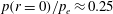 $p(r=0)/p_{e}\approx 0.25$
. For an aluminium plate with a thickness
$p(r=0)/p_{e}\approx 0.25$
. For an aluminium plate with a thickness
 $b=4~\text{cm}$
, bending rigidity
$b=4~\text{cm}$
, bending rigidity
 $s=10^{7}~\text{Pa}~\text{m}^{3}$
, gap
$s=10^{7}~\text{Pa}~\text{m}^{3}$
, gap
 $h_{0}=1~\text{mm}$
and liquid viscosity
$h_{0}=1~\text{mm}$
and liquid viscosity
 ${\it\mu}=60~\text{Pa}~\text{s}$
(silicon oil), external force of
${\it\mu}=60~\text{Pa}~\text{s}$
(silicon oil), external force of
 $10^{5}~\text{N}$
applied uniformly on a disk of radius
$10^{5}~\text{N}$
applied uniformly on a disk of radius
 $l_{e}=1~\text{cm}$
and gradually increasing over
$l_{e}=1~\text{cm}$
and gradually increasing over
 $t_{e,2}=10^{-4}~\text{s}$
yields signal propagation velocity of
$t_{e,2}=10^{-4}~\text{s}$
yields signal propagation velocity of
 ${\approx}300~\text{m}~\text{s}^{-1}$
and impact mitigation of
${\approx}300~\text{m}~\text{s}^{-1}$
and impact mitigation of
 $p(r=0)/p_{e}\approx 0.03$
.
$p(r=0)/p_{e}\approx 0.03$
.
Acknowledgement
This research was supported by the Israel Science Foundation (grant no. 818/13). We thank Mr A. Tahar for constructing and conducting the experiments, as well as taking part in their design.
Appendix A. Results in dimensional form
Presented here are some of the equations and results in dimensional form. These include the Green’s equation
 $$\begin{eqnarray}{\displaystyle \frac{\partial g}{\partial t}}-{\displaystyle \frac{h_{0}^{3}s}{12{\it\mu}}}{\rm\nabla}^{6}g={\it\delta}(x){\it\delta}(y){\it\delta}(t),\end{eqnarray}$$
the governing equation for deformation (2.13)
 $$\begin{eqnarray}{\displaystyle \frac{\partial d}{\partial t}}-{\displaystyle \frac{h_{0}^{3}s}{12{\it\mu}}}{\rm\nabla}^{6}d={\displaystyle \frac{h_{0}^{3}}{12{\it\mu}}}{\rm\nabla}^{2}p_{e},\end{eqnarray}$$
the governing equation for pressure (2.14)
 $$\begin{eqnarray}{\displaystyle \frac{\partial p}{\partial t}}-{\displaystyle \frac{h_{0}^{3}s}{12{\it\mu}}}{\rm\nabla}^{6}p={\displaystyle \frac{\partial p_{e}}{\partial t}},\end{eqnarray}$$
the Green’s function for (A 1)
 $$\begin{eqnarray}g({\it\eta},t)=\left({\displaystyle \frac{h_{0}^{3}s}{12{\it\mu}}}\right)^{-1/3}{\displaystyle \frac{{\it\Psi}({\it\eta})}{t^{1/3}}},\end{eqnarray}$$
the Green’s function for deformation (A 2)
 $$\begin{eqnarray}g_{d}({\it\eta},t)=\left({\displaystyle \frac{h_{0}^{3}s}{12{\it\mu}}}\right)^{-2/3}{\displaystyle \frac{{\it\Psi}_{d}({\it\eta})}{t^{2/3}}}\end{eqnarray}$$
the Green’s function for pressure (A 3)
 $$\begin{eqnarray}g_{p}({\it\eta},t)=\left({\displaystyle \frac{h_{0}^{3}s}{12{\it\mu}}}\right)^{-1/3}{\displaystyle \frac{{\it\Psi}_{p}({\it\eta})}{t^{4/3}}},\end{eqnarray}$$
where
 ${\it\eta}$
for (A 2–A 6) is
${\it\eta}$
for (A 2–A 6) is
 $$\begin{eqnarray}{\it\eta}=\left({\displaystyle \frac{h_{0}^{3}s}{12{\it\mu}}}\right)^{-1/6}{\displaystyle \frac{|\boldsymbol{x}|}{6t^{1/6}}}.\end{eqnarray}$$
The deformation and pressure distribution as a result of a specific external pressure,
 $p_{e}=p_{e}(x,y,t)$
, are obtained by the convolutions
$p_{e}=p_{e}(x,y,t)$
, are obtained by the convolutions
 $$\begin{eqnarray}d={\displaystyle \frac{h_{0}^{3}}{12{\it\mu}}}\int _{0}^{t}\int _{-\infty }^{\infty }\int _{-\infty }^{\infty }g_{d}(x-\bar{x},y-\bar{y},t-\bar{t})p_{e}(\bar{x},\bar{y},\bar{t})\,\text{d}\bar{x}\,\text{d}\bar{y}\,\text{d}\bar{t}\end{eqnarray}$$
and
 $$\begin{eqnarray}p=\int _{0}^{t}\int _{-\infty }^{\infty }\int _{-\infty }^{\infty }g_{p}(x-\bar{x},y-\bar{y},t-\bar{t})p_{e}(\bar{x},\bar{y},\bar{t})\,\text{d}\bar{x}\,\text{d}\bar{y}\,\text{d}\bar{t}.\end{eqnarray}$$


