


1. Introduction
Liquid cylinders, jets or annular liquid films coating rods often deform or fragment into a series of droplets of unequal sizes via the ubiquitous Rayleigh–Plateau (RP) capillary mechanism (Plateau Reference Plateau1873b; Rayleigh Reference Rayleigh1892b). This may easily be seen, for example, in a jet issuing out of a faucet (Rutland & Jameson Reference Rutland and Jameson1971), in a capillary liquid bridge held between two disks (Plateau Reference Plateau1873b) or in a film coating a rod (Goren Reference Goren1962), to mention but a few situations. Depending on the application, droplet formation may be desirable or it might even be necessary to suppress it. When breakup is intended (e.g. in microfluidic devices cf. Stone, Stroock & Ajdari (Reference Stone, Stroock and Ajdari2004) or drop-on-demand inkjet printing cf. Driessen Reference Driessen2013), strategies are sought such that the size distribution of the resultant droplets and their spacing are controllable, e.g. Driessen et al. (Reference Driessen, Sleutel, Dijksman, Jeurissen and Lohse2014). Conversely, when breakup is undesirable, stabilisation strategies are necessary and a number of techniques have been proposed towards this. Table 1 provides a broad summary of known techniques of RP stabilisation and it is apparent that this continues to be an active area of research.
Table 1. Literature on RP mode stabilisation.

The purpose of the present study is to demonstrate dynamic stabilisation of unstable RP modes on a liquid cylinder by subjecting the cylinder to a radial, sinusoidal-in-time body force. It is demonstrated analytically that this is possible and that viscosity plays a crucial role in this stabilisation. The viscous analysis presented here significantly builds upon the inviscid analysis presented earlier in Patankar, Farsoiya & Dasgupta (Reference Patankar, Farsoiya and Dasgupta2018) where dynamic (quasi-stabilisation) of RP modes was also predicted but the quasi-stabilisation was found to be extremely short-lived in inviscid simulations. In contrast to our earlier inviscid study (Patankar et al. Reference Patankar, Farsoiya and Dasgupta2018), we demonstrate here that, for a viscous liquid, by carefully tuning the strength and frequency of (radial) forcing, RP modes accessible to the system may be rendered stable, thus stabilising the cylinder. The theoretically predicted stabilisation is verified using numerical simulations of the Navier–Stokes equations demonstrating excellent agreement (up to the simulation time of several hundred forcing cycles).
The study is organised as follows. In § 1.1 a brief literature survey discussing the gamut of stabilisation strategies for finite and infinitely long liquid cylinders along with a brief background of parametric instabilities and dynamic stabilisation strategies is presented. In § 2 linear stability analysis of an infinite cylinder of viscous liquid subject to a radial, oscillatory body force is reported via Floquet analysis. Section 3 reports the derivation of a novel integro-differential equation governing the linearised amplitude of surface modes. The theoretically predicted stabilisation in § 4 is verified using numerical simulations of the incompressible Navier–Stokes equations (DNS) in § 5. The integro-differential equation is physical interpreted and the significance of the memory term is discussed at the end of § 5. Conclusions are discussed in § 6.
1.1. Literature review
Stabilisation of RP modes for liquid cylinders are typically investigated either in the context of bridges of finite length or in the infinitely long cylinder approximation. We recall that a cylindrical liquid bridge of length  $L$ and diameter
  $d$ in neutrally buoyant surroundings is stable for slenderness ratio
  $L/d \leq {\rm \pi}$, also known as the Plateau limit; see Plateau (Reference Plateau1873a). An electric field has long been used to both generate stable cylindrical jets (Taylor Reference Taylor1969) and to stabilise liquid bridges composed of dielectric fluids (Raco Reference Raco1968; Sankaran & Saville Reference Sankaran and Saville1993; Thiessen, Marr-Lyon & Marston Reference Thiessen, Marr-Lyon and Marston2002). Alternatively, application of axial magnetic fields (Nicolás Reference Nicolás1992) or flow induced stabilisation techniques (Lowry & Steen Reference Lowry and Steen1994, Reference Lowry and Steen1995, Reference Lowry and Steen1997) have been utilised for surmounting the Plateau limit, obtaining stabilisation up to
  $L/R=8.99$ for a pinned liquid bridge. Another class of techniques comprise acoustic forcing, which has been used to demonstrate stabilisation of liquid bridges beyond the Plateau limit (Marr-Lyon, Thiessen & Marston Reference Marr-Lyon, Thiessen and Marston1997, Reference Marr-Lyon, Thiessen and Marston2001). The nonlinear dynamics of liquid bridges and their stability subject to axial, oscillatory forcing of the point of support have in fact been studied quite extensively (Chen & Tsamopoulos Reference Chen and Tsamopoulos1993; Mollot et al. Reference Mollot, Tsamopoulos, Chen and Ashgriz1993; Benilov Reference Benilov2016; Haynes et al. Reference Haynes, Vega, Herrada, Benilov and Montanero2018). Analogously, the use of axial vibration for stabilising and preventing rupture of a thin film coating a solid rod by subjecting one end of the rod to ultrasound forcing has been investigated in detail (Moldavsky, Fichman & Oron Reference Moldavsky, Fichman and Oron2007; Binz, Rohlfs & Kneer Reference Binz, Rohlfs and Kneer2014; Rohlfs, Binz & Kneer Reference Rohlfs, Binz and Kneer2014). Parametric stabilisation, also known as dynamic stabilisation, via imposition of vibration has been demonstrated (Wolf Reference Wolf1970) for the Rayleigh–Taylor instability of a heavier fluid overlying a lighter one. Here viscosity was found to be crucial for stabilisation of short wavelength modes. In this study we will find that an identical situation occurs in the dynamic stabilisation of RP modes also. Here short wavelength modes (i.e. those with wavelength smaller than the cylinder circumference) which are stable in the absence of forcing can however become unstable in the presence of forcing. These modes, even when absent in the initial conditions, can be produced due to nonlinearity (in numerical simulations) and it will be seen that viscosity is crucial in preventing destabilisation of the cylinder due to these modes.
Parametric stabilisation and destabilisation of otherwise unstable or stable mechanical equilibria have a long and distinguished history of investigation. The first problems to be investigated were mechanical systems, notably by Melde (Reference Melde1860) who studied transverse oscillations of a taut string whose end was subjected to lengthwise vibrations (see Tyndall Reference Tyndall1901, § 7, figures 45–49). In a series of studies Rayleigh (Reference Rayleigh1883, Reference Rayleigh1887), Matthiessen (Reference Matthiessen1868) and Raman (Reference Raman1909, Reference Raman1912) studied this problem in detail obtaining the damped Mathieu equation already in their analyses. Closely related experimental observations for fluid interfaces (using mercury, egg white, turpentine oil etc.) had been made nearly thirty years earlier by Faraday (Reference Faraday1837) culminating in the insightful study by Benjamin & Ursell (Reference Benjamin and Ursell1954) of the instability, which in modern parlance has come to be known as the Faraday instability.
Benjamin & Ursell (Reference Benjamin and Ursell1954) derived the Mathieu equation from the inviscid, irrotational fluid equations opening the way to a rich body of literature on Faraday waves (Kumar & Tuckerman Reference Kumar and Tuckerman1994; Cerda & Tirapegui Reference Cerda and Tirapegui1997; Fauve Reference Fauve1998; Kumar Reference Kumar2000; Adou & Tuckerman Reference Adou and Tuckerman2016), spatio-temporal chaos (Kudrolli & Gollub Reference Kudrolli and Gollub1996), wave turbulence (Holt & Trinh Reference Holt and Trinh1996; Shats et al. Reference Shats, Francois, Xia and Punzmann2014) and pattern formation (Edwards & Fauve Reference Edwards and Fauve1994; Arbell & Fineberg Reference Arbell and Fineberg2000). Viscosity constitutes a non-trivial modification to the Mathieu equation. Unlike inviscid predictions on the forcing strength vs wavenumber plane, the threshold acceleration for the instability becomes finite when viscosity is taken into account, as the instability tongues do not touch the wavenumber axis anymore. This was first systematically demonstrated by Kumar & Tuckerman (Reference Kumar and Tuckerman1994) using Floquet analysis, further finding that the wavelength at the onset of the instability varies non-monotonically with increasing viscosity. The predictions of Kumar & Tuckerman (Reference Kumar and Tuckerman1994) have been validated in experiments by Bechhoefer et al. (Reference Bechhoefer, Ego, Manneville and Johnson1995) and, for Faraday waves, in a cylinder by Batson, Zoueshtiagh & Narayanan (Reference Batson, Zoueshtiagh and Narayanan2013).
The stability tongues of the Mathieu equation suggest the possibility of dynamic stabilisation of a statically unstable configuration of heavier fluid on a top of a lighter one via high-frequency oscillation normal to the unperturbed interface. Since the theoretical and experimental demonstration of this by Wolf (Reference Wolf1969, Reference Wolf1970), this has been studied extensively not only for the Rayleigh–Taylor instability (Troyon & Gruber Reference Troyon and Gruber1971; Piriz et al. Reference Piriz, Prieto, Diaz, Cela and Tahir2010; Boffetta, Magnani & Musacchio Reference Boffetta, Magnani and Musacchio2019) but also in the suppression of long surface-gravity modes in inclined plane flow (Woods & Lin Reference Woods and Lin1995), the Marangoni instability (Thiele, Vega & Knobloch Reference Thiele, Vega and Knobloch2006) and for stabilising a thin film on the underside of a substrate (Sterman-Cohen, Bestehorn & Oron Reference Sterman-Cohen, Bestehorn and Oron2017). In close analogy to the work of Wolf (Reference Wolf1970), our present study demonstrates usage of radial forcing (i.e. normal to the unperturbed interface) for dynamic stabilisation of RP modes. In § 4.1 we present a detailed discussion and comparison with the experiments of Maity, Kumar & Khastgir (Reference Maity, Kumar and Khastgir2020) for a liquid cylinder on a vertically vibrated substrate, where the radial, oscillatory body force employed in our theory is approximately realized. To the best of our knowledge, our study is the first theoretical and numerical demonstration of dynamic stabilisation of a liquid cylinder (a condensed version was presented in Patankar, Basak & Dasgupta (Reference Patankar, Basak and Dasgupta2019), Patankar et al. (Reference Patankar, Basak, Farsoiya and Dasgupta2020) and an earlier version of this manuscript is available at arxiv, Patankar, Basak & Dasgupta Reference Patankar, Basak and Dasgupta2022). We closely follow the Floquet analysis approach of Kumar & Tuckerman (Reference Kumar and Tuckerman1994) in order to obtain the threshold forcing where RP mode stabilisation can be achieved. For viscous liquid cylinders, a recent study by Maity (Reference Maity2021) has investigated via Floquet analysis the effect of viscosity on the stability tongues of the inviscid Mathieu equation proposed in Patankar et al. (Reference Patankar, Farsoiya and Dasgupta2018), and investigated further experimentally and analytically in Maity et al. (Reference Maity, Kumar and Khastgir2020). An interesting observation here is that the  $m=1$ mode shows a threshold which decreases with increasing viscosity, in a certain window of viscosity change (Maity Reference Maity2021). The study by Maity (Reference Maity2021) however did not investigate the possibility of stabilisation of RP unstable modes, as is the focus of the current study. We note here that the theoretical analysis to follow assumes that the liquid cylinder is axially unbounded, this assumption being made mainly for theoretical simplication. As we will see in § 4.1, our theoretical results are also relevant to RP unstable modes on cylindrical rivulets placed on substrates.
For Faraday waves on flat interfaces, prior studies have demonstrated that the viscous extension of the inviscid Mathieu equation (Benjamin & Ursell Reference Benjamin and Ursell1954) is an integro-differential equation (Jacqmin & Duval Reference Jacqmin and Duval1988; Beyer & Friedrich Reference Beyer and Friedrich1995; Cerda & Tirapegui Reference Cerda and Tirapegui1997, Reference Cerda and Tirapegui1998). In this study we also derive a novel cylindrical analogue of this integro-differential equation governing small-amplitude Fourier modes on a liquid cylinder and demonstrate its connection to the equation derived earlier by Beyer & Friedrich (Reference Beyer and Friedrich1995). Numerical solution to this integro-differential equation enables us to estimate the contribution of viscosity from the potential part of the flow and from the boundary layer at the free surface. Additionally, the solution to this equation demonstrates the RP stabilisation that is sought is in excellent agreement with direct numerical simulations (DNS).
2. Linear stability analysis
The base state comprises an infinitely long, quiescent liquid cylinder of density  $\rho$, surface tension
  $T$, kinematic viscosity
  $\nu$ and radius
  $R_0$ being subject to a radial, oscillatory body force
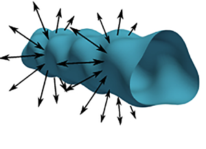
  $\mathcal {F}(r,t)$; see figure 1. This radial body force (per unit mass) has strength
  $h$ and a spatial dependence of the form
  ${r}/{R_0}$ in order to ensure single valuedness of the force at the origin (Adou & Tuckerman Reference Adou and Tuckerman2016; Patankar et al. Reference Patankar, Farsoiya and Dasgupta2018), and the negative sign in the expression for
  $\mathcal {F}(r,t)$ is for convenience (see below (2.1)). Thus, in the base state (variables with subscript
  $b$) there is no flow, the interface is a uniform cylinder of radius
  $R_0$ and the momentum equation simplifies to a balance between the radial oscillatory body force and the pressure gradient, viz.
 \begin{gather} \left. \begin{gathered} \boldsymbol{u}_b = 0,\quad -\frac{1}{\rho}\boldsymbol{\nabla}p_b + \mathcal{F}(r,t)\hat{\boldsymbol{e}}_r = 0,\quad 0 \leq r \leq R_0,\\ \text{with} \ \mathcal{F}(r,t) \equiv{-}h\left(\frac{r}{R_0}\right)\cos\left(\varOmega t\right),\quad \text{and}\quad p_b(r,t) = \frac{\rho h}{2R_0}(R_0^2-r^2)\cos(\varOmega t) + \frac{T}{R_0}. \end{gathered} \right\} \end{gather}
Here  $\boldsymbol {\hat {e}}_r$ is the standard unit vector in the radial direction in cylindrical coordinates. Note that we have assumed stress in the fluid outside the cylinder to be zero, so that
  $p_b(R_0,t) = {T}/{R_0}$ satisfies the pressure jump condition at the interface due to surface tension. We neglect the density and viscosity of the fluid outside in the present study implying that the free surface of the cylinder satisfies stress free conditions. In the following subsection we briefly discuss RP modes in the unforced system (
 $h=0$), followed by an inviscid and viscous description of RP stabilisation with radial forcing (
 $h\neq 0$).

Figure 1. A cartoon of a surface perturbation on a viscous liquid cylinder of radius  $R_0$ subject to a radial body force
  $\boldsymbol {\mathcal {F}}(r,t) = \mathcal {F}(r,t)\boldsymbol {\hat {e}}_r= -h({r}/{R_0})\cos (\varOmega t)\boldsymbol {\hat {e}}_r$. The variable
  $\eta (\theta,z,t)$ measures the displacement of the free surface with respect to the unperturbed cylinder, being zero in the base state. Surface perturbations
  $\eta (\theta,z,t) = a_m(t;k)\cos (m\theta )\cos (kz)$ are imposed.
2.1. The inviscid and viscous RP modes ( $h=0$)

The classical RP modes are unstable axisymmetric Fourier modes satisfying  $0 < kR_0 < 1$ for the unforced system (
 $h=0$). These are governed by the following inviscid ((2.2a), Rayleigh Reference Rayleigh1878) and viscous dispersion relation (Rayleigh Reference Rayleigh1892a; Weber Reference Weber1931; Chandrasekhar Reference Chandrasekhar1981; Liu & Liu Reference Liu and Liu2006) with growth rate
  $\sigma _0$ (inviscid) and
  $\sigma$ (viscous), respectively:
 \begin{gather} \sigma_0^2 = \frac{T}{\rho R_0^3}kR_0(1 - k^2R_0^2)\frac{{\mathrm{I}}_1(kR_0)}{{\mathrm{I}}_0(kR_0)}, \end{gather}
 \begin{gather} \left. \begin{gathered} \sigma^{2}+2 v k^{2}\left[\frac{{\mathrm{I}}_{1}^{\prime}(k R_{0})}{{\mathrm{I}}_{0}(k R_{0})}-\frac{2 k l}{l^{2}+k^{2}} \frac{{\mathrm{I}}_{1}(k R_{0})}{{\mathrm{I}}_{0}(k R_{0})} \frac{{\mathrm{I}}_{1}^{\prime}(l R_{0})}{{\mathrm{I}}_{1}(l R_{0})}\right]\sigma - \left(\frac{l^{2}-k^{2}}{l^{2}+k^{2}}\right)\sigma_0^2 = 0,\\ \text{where}\quad l^2 \equiv k^2 + \frac{\sigma}{\nu}. \end{gathered} \right\} \end{gather}
Here  ${\mathrm {I}}_{m}(z)$ is the
  $m$th order modified Bessel function of the first kind and
  ${\mathrm {I}}_{m}^{'}(z) \equiv {\textrm {d}{\mathrm {I}}_m}/{\textrm {d}z}$. In figure 2,
  $\sigma _0$ and
  $\sigma$ are obtained by numerically solving (2.2a) and (2.2b) for the inviscid and viscous cases, respectively. Unlike the inviscid relation (2.2a) which is quadratic in
  $\sigma _0$, the viscous dispersion relation given by (2.2b) is transcendental in
  $\sigma$. It admits in addition to two capillary modes, a countably infinite set of hydrodynamic (or vorticity) modes as its roots and the latter are purely damped modes (García & González Reference García and González2008). In figure 2 we only depict the growth and decay rates corresponding to the two capillary modes in the range
  $0 < kR_0 < 1$ for different values of Ohnesorge number
  ${Oh} = {\mu }/{\sqrt {T\rho R_0}}$. Our aim in this study is to stabilise the capillary modes in the range
  $0 < kR_0 < 1$ using radial forcing and this is discussed below.

Figure 2. Inviscid and viscous growth (and decay) rates of RP modes ( $0 < kR_0 < 1$) from numerically solving (2.2a) and (2.2b) (Weber Reference Weber1931; García & González Reference García and González2008). At any Ohnesorge (
 $Oh$) and
  $k$ in the range
  $0 < k < R_0^{-1}$, there are two capillary modes, one unstable (
 $\sigma > 0$) and another stable
  $(\sigma < 0)$. We stabilise the exponentially growing mode by forcing at
  $\varOmega \gg \sigma _{max}$, where
  $\sigma _{max}$ is the growth rate of the fastest growing RP mode, it being highest for the inviscid case (
 $Oh=0$) for
  $(kR_0)_{max} \approx 0.69$ with
  $\sigma _{{max}} \approx 0.34\sqrt {{T}/{\rho R_0^3}}$.
2.2. Dynamic stabilisation of RP modes – linear inviscid theory
The inviscid results on RP stabilisation using radial forcing were presented earlier in Patankar et al. (Reference Patankar, Farsoiya and Dasgupta2018) and are summarised very briefly here, for self-containedness. In the presence of radial forcing  $\mathcal {F}(r,t) = -h({r}/{R_0})\cos (\varOmega t)$ and under the linearised, inviscid, irrotational approximation, the equation governing the amplitude
  $a_m(t;k)$ of standing waves on the free surface of the form
  $\eta (z,\theta,t) = a_m(t;k)\cos (m\theta )\cos (kz)$ is the Mathieu equation (2.3)
 \begin{equation} \frac{{\rm d}^2a_m}{{\rm d}t^2} + \frac{{\mathrm{I}}^{'}_{m}\left(kR_0\right)}{{\mathrm{I}}_{m}\left(kR_0\right)}\left[\frac{T}{\rho R_0^3}kR_0\left(k^2R_0^2 + m^2 -1\right) + kh\cos(\varOmega t)\right] a_m(t;k) = 0. \end{equation}
The stability diagram for (2.3) may be obtained using Floquet analysis (Patankar et al. Reference Patankar, Farsoiya and Dasgupta2018). For  $h \neq 0$, we have the interesting prediction that axisymmetric unstable RP modes can be stabilised by choosing
  $h$ to be sufficiently large. This is readily seen in the stability chart in figure 3(a) where the solid curve in black indicates the threshold value of forcing
  $h$ above which, a RP mode is stable. The line in blue indicates all unstable RP modes for
  $h=0$. Two representative RP unstable modes are chosen, viz.
  $k_0=4.8$ cm
 $^{-1}$ (wavelength
  $\lambda \approx 1.309$ cm) and
  $k_0=3.48$ cm
 $^{-1}$ (
 $\lambda \approx 1.8$ cm) . The plot predicts the threshold values of forcing strength
  $h_{{cr}}=1.21\times 10^4\, \textrm {cm}\,\textrm {s}^{-2}$ and
  $h_{{cr}}=4.17\times 10^4\, \textrm {cm}\,\textrm {s}^{-2}$, respectively, beyond which these modes can be stabilised. For generating figure 3(a), we have chosen
  $\varOmega = 600 {\rm \pi}\,\textrm {rad}\,\textrm {s}^{-1}$ (
 $f=300$ Hz),
  $R_0=0.2$ cm, density
  $\rho =0.957\,\textrm {gm}\,\textrm {cm}^{-3}$, surface tension
  $T=20.7\,\textrm {dyn}\,\textrm {cm}^{-1}$. These fluid parameters approximately correspond to silicone oil (Vega & Montanero Reference Vega and Montanero2009) with its viscosity artificially set to zero. Note that at these forcing frequencies we may safely ignore compressibility effects as may be inferred from the order of magnitude of the two typical velocity scales, viz.
  $\textrm {maximum}[{h_{c}}/{f},fR_0] \approx 139\,\textrm {cm}\,\textrm {s}^{-1}$ for
  $f=300$ Hz and
  $h_c=4.17\times 10^4\, \textrm {cm}\,\textrm {s}^{-2}$. This is negligible compared with the typical acoustic speed
  ${O}(10^5)\,\textrm {cm}\,\textrm {s}^{-1}$ in the fluid at ambient conditions.

Figure 3. Grey and white indicate unstable and stable regions, respectively. Panel (a) shows the inviscid stability chart for (2.3). The forcing frequency  $f = 300\,\textrm {Hz} \gg \sigma _{{max}}= 0.34\sqrt {T/(\rho R_0^3)} = 17.68\,\textrm {Hz}$. Parameters are for case 1 in table 3 with
  $\mu ^{I}=0$. Panel (b) shows the time signal (red curve) from the numerical solution to the 3-D Euler equation (Popinet Reference Popinet2014) with an RP mode (
 $k_0=4.8\,\textrm {cm}^{-1},m_0=0$) excited at
  $t=0$. Black curve: solution to (2.3). Left inset: zoomed out view of solution to (2.3). Right inset: stability chart for
  $m=4$. An unstable non-axisymmetric Fourier mode (
 $k=28.8=6k_0,m=4$ in the grey region) at
  $\tilde {t} \approx 14$ s causes destabilisation of the cylinder. (a) Stability plot. (b) Result shown for
  $k=4.8,h= 1.8\times 10^4\, \textrm {cm}\,\textrm {s}^{-2}$.
The results from the numerical simulations discussed below are obtained using the open-source code Basilisk (Popinet Reference Popinet2014). The simulations are described in detail later on in § 5 and are briefly discussed here for consistency. The domain consists of a liquid cylinder of silicone oil surrounded by an ambient fluid of negligible density and viscosity (see figure 7 in § 5). The cylinder is subjected to a radial harmonic (in time) forcing. The simulation parameters for the case discussed below correspond to case  $1$ from table 3 with
  $\mu ^{I} = \mu ^{O} = 0$ to reflect the inviscid limit that we analyse first. Figure 3(b) presents the time signal obtained from inviscid numerical simulations (Popinet Reference Popinet2014) for the axisymmetric mode
  $k_0=4.8,m_0=0$ excited at
  $t=0$. Note that this is a RP unstable mode and as seen from figure 3(a), it is expected to be stabilised beyond a threshold forcing of
  $h=1.21\times 10^4\, \textrm {cm}\,\textrm {s}^{-2}$. In figure 3(b) we see agreement between the solution to (2.3) and the numerical simulation for very brief time (approximately three forcing time periods), after which the signal from the numerical simulation begins to deviate and grow rapidly (around
  $\tilde {t}\approx 14$) in contrast to the solution to (2.3) which stays bounded (see left inset). A Fourier analysis of the interface at
  $\tilde {t} \equiv t\varOmega /2{\rm \pi} \approx 14$, indicated by the arrow, reveals the appearance of a non-axisymmetric mode
  $(k=28.8,m=4)$ in the simulation. This is a stable mode in the unforced system (
 $h=0$) but is destabilised at the imposed level of forcing, lying inside a tongue as seen in the right inset of figure 3(b). Thus, in the inviscid case the stabilisation that is achieved is only a quasi-stabilisation in the sense that while the RP modes can be rendered stable via forcing, concomitantly, other modes become unstable at the chosen level of forcing. It thus becomes clear that for obtaining dynamic stabilisation, we need to ensure that all Fourier modes either present initially in the system or born via nonlinear effects, both axisymmetric and three dimensional, should remain linearly stable at the imposed level of forcing. We will demonstrate in the next section that by taking viscosity into account and using the forcing frequency as a tuning parameter, this may be achieved.
2.3. Dynamic stabilisation of RP modes – linear viscous theory
Having demonstrated the inadequacy of dynamic stabilisation of RP modes in an inviscid model, we proceed to the viscous case. The motivation for including viscosity is simple to understand: it is known that inclusion of viscosity leads to displacement of the instability tongues upwards on the  $h$–
$h$– $k$ plane and these no longer touch the wavenumber axis (Kumar & Tuckerman Reference Kumar and Tuckerman1994). Our expectation is that by suitably choosing viscosity and the forcing frequency, we will be able to shift the unstable tongues sufficiently above the wavenumber (
 $k$) axis. This generates a sufficiently large stable region where not only the axisymmetric RP unstable mode (
 $k_0$) is stabilised (with forcing) but all higher modes accessible to the system are also stable. Note that the upward movement of the tongues occur not only for axisymmetric modes but also for non-axisymmetric ones. In particular, we will also see that for fixed viscosity, we can move the minima of the tongue upwards by increasing the forcing frequency. The algebra for the viscous analysis is somewhat lengthy and details are provided in the supplementary material available at https://doi.org/10.1017/jfm.2022.533. We outline the important steps that follow. Expressing all quantities as the sum of base plus perturbation, i.e.
 \begin{equation} \hat{p} = p_b + p,\quad \hat{\boldsymbol{u}} = \boldsymbol{0} + \boldsymbol{u}\quad \text{and} \quad \text{perturbed free surface at}\ r = R_0 + \eta. \end{equation}
Substituting (2.4a,b) into the incompressible Navier–Stokes equations and linearising about the base state we obtain the equations governing the perturbations, viz.
 \begin{equation} \left(\frac{\partial}{\partial t} - \nu \Delta\right)\boldsymbol{u} ={-}\frac{1}{\rho}\boldsymbol{\nabla}p,\quad \boldsymbol{\nabla}\boldsymbol{{\cdot}}\boldsymbol{u} = 0, \end{equation}
where the vector Laplacian of the incompressible velocity field is  $\Delta \boldsymbol {u} \equiv -\boldsymbol {\nabla }\times \boldsymbol {\nabla }\times \boldsymbol {u}$. The linearised boundary conditions are obtained by substituting (2.4a–c) into the boundary conditions (supplementary material), employing Taylor expansion and retaining terms linear in the perturbation variables, viz.
  $\boldsymbol {u}, p$ and
  $\eta$ (the perturbation velocity
  $\boldsymbol {u}$ is written in terms of its components
  $(u_r,u_{\theta },u_z)$), we obtain
 \begin{gather} \frac{\partial\eta}{\partial t} = u_r(r=R_0), \end{gather}
 \begin{gather} \mu\left(\frac{\partial u_r}{\partial z} + \frac{\partial u_z}{\partial r}\right)_{r=R_0} = 0, \quad \mu\left(r\frac{\partial}{\partial r}\left(\frac{u_{\theta}}{r}\right) + \frac{1}{r}\frac{\partial u_r}{\partial \theta}\right)_{r=R_0} = 0, \end{gather}
 \begin{gather} \left. \begin{aligned} & \left( \frac{\partial}{\partial r} + \frac{1}{r}\right)\left[\frac{\partial u_r}{\partial t} - \nu\left\{\Delta u_r - \frac{u_r}{r^2} - \frac{2}{r^2}\left(\frac{\partial u_{\theta}}{\partial\theta}\right)\right\}\right] +\mathcal{F}(r,t)\Delta_O\eta - 2\nu\Delta_O\left(\frac{\partial u_r}{\partial r}\right) \\ & \qquad ={-}\frac{T}{\rho R_0^2}\Delta_O\left[\eta + \left(\frac{\partial^2\eta}{\partial \theta^2}\right) + R_0^2\left(\frac{\partial^2\eta}{\partial z^2}\right)\right] \quad \text{at} r=R_0,\\ & \quad \text{with}\quad\Delta_{O} \equiv \frac{1}{r^2}\frac{\partial^2}{\partial \theta^2} + \frac{\partial^2}{\partial z^2}, \end{aligned} \right\} \end{gather}
 \begin{gather} \boldsymbol{u}(r\rightarrow 0 ,t)\rightarrow \text{finite}, \end{gather}
where  $\Delta$ is the scalar Laplacian in cylindrical coordinates. Equations (2.6a–e) are the linearised versions of the kinematic boundary condition (2.6a), the zero shear stress condition(s) at the free surface (2.6b,c), the normal stress condition at the free surface due to surface tension (2.6d) and the finiteness condition at the axis of the cylinder (2.6e), respectively. Equation (2.6d) has been obtained by eliminating pressure from the primitive form of the pressure jump boundary condition (see supplementary material). Note the presence of the forcing term
  $\mathcal {F}(r,t)$ in the normal stress boundary condition in (2.6d) indicating the time periodicity of the base state.
We solve (2.5a,b) in the streamfunction-vorticity formulation and, for this, the curl and double curl of (2.5a) leads to ( $\boldsymbol {\omega } \equiv \boldsymbol {\nabla }\times \boldsymbol {u}$)
 \begin{equation} \frac{\partial\boldsymbol{\omega}}{\partial t} = \nu\boldsymbol{\Delta}\boldsymbol{\omega},\quad \frac{\partial}{\partial t}\boldsymbol{\Delta} \boldsymbol{u} = \nu \boldsymbol{\Delta} \boldsymbol{\Delta} \boldsymbol{u}, \end{equation}
where  $\boldsymbol {\Delta }$ is the vector Laplacian. Employing the toroidal-poloidal decomposition (Marqués Reference Marqués1990; Boronski & Tuckerman Reference Boronski and Tuckerman2007; Prosperetti Reference Prosperetti2011), the velocity and vorticity fields are expressed in terms of two scalar fields
  $\psi (r,\theta,z,t)$ and
  $\xi (r,\theta,z,t)$ using the decomposition
 \begin{align} \boldsymbol{u} = \boldsymbol{\nabla}\times\left(\psi\hat{\boldsymbol{e}}_z\right) + \boldsymbol{\nabla}\times\boldsymbol{\nabla}\times\left(\xi\hat{\boldsymbol{e}}_z\right),\quad \boldsymbol{\omega} \equiv \boldsymbol{\nabla}\times\boldsymbol{\nabla}\times\left(\psi\hat{\boldsymbol{e}}_z\right) + \boldsymbol{\nabla}\times\boldsymbol{\nabla}\times\boldsymbol{\nabla}\times\left(\xi\hat{\boldsymbol{e}}_z\right), \end{align}
where  $\hat {\boldsymbol {e}}_z$ is the unit vector along the axial direction of the cylinder (Boronski & Tuckerman Reference Boronski and Tuckerman2007). By construction the velocity field in (2.8a) is divergence free and it can be shown (see supplementary material) that the equations governing the toroidal and poloidal fields
  $\psi (r,z,\theta,t)$ and
  $\xi (r,z,\theta,t)$, respectively, are the fourth- and sixth-order equations
 \begin{equation} \left(\frac{\partial}{\partial t} - \nu\Delta\right)\Delta_{{H}}\psi = 0 \quad \text{and}\quad \left(\frac{\partial}{\partial t} - \nu\Delta\right)\Delta\Delta_{{H}}\xi = 0, \end{equation}
where the scalar Laplacian
 \begin{equation} \Delta \equiv \frac{1}{r}\frac{\partial}{\partial r}(r\frac{\partial}{\partial r}) + \frac{1}{r^2}\frac{\partial^2}{\partial\theta^2} + \frac{\partial^2}{\partial z^2}= \Delta_{{H}} + \frac{\partial^2}{\partial z^2}. \end{equation}
As we have raised the order of our governing equations by taking curl and double curl, we need extra equations to determine the additional constants of integration. It was shown in Marqués (Reference Marqués1990) that this takes the form of an additional equation also known as the compatibility condition (Boronski & Tuckerman Reference Boronski and Tuckerman2007). For the present problem at linear order, this extra equation is simply the radial component of the vorticity equation (2.7a) (Boronski & Tuckerman Reference Boronski and Tuckerman2007), i.e.
 \begin{equation} \left. \begin{gathered} \dfrac{\partial \omega_r}{\partial t} = \nu\left\{\Delta \omega_r - \dfrac{\omega_r}{r^2} - \dfrac{2}{r^2}\left(\dfrac{\partial \omega_{\theta}}{\partial\theta}\right)\right\}, \\ \text{with}\quad \omega_r = \dfrac{\partial^2 \psi}{\partial r \partial z } -\dfrac{1}{r}\dfrac{\partial}{\partial\theta}\left(\Delta \xi \right) \quad \text{and} \quad \omega_\theta=\dfrac{1}{r}\dfrac{\partial^2 \psi}{\partial z \partial \theta } + \dfrac{\partial}{\partial r}\left(\Delta \xi\right). \end{gathered} \right\} \end{equation}
In order to determine the scalar fields  $\psi (r,\theta,z,t), \xi (r,\theta,z,t)$, we need to solve (2.9a,b). Analogous to the inviscid analysis in Patankar et al. (Reference Patankar, Farsoiya and Dasgupta2018) we seek three-dimensional standing wave solutions of the form
 $$\begin{gather} \psi(r,\theta,z,t) = \varPsi_m(r,t;k)\sin(m\theta)\cos(kz),\quad\xi(r,\theta,z,t) = \varXi_m(r,t;k)\cos(m\theta)\sin(kz), \nonumber\\ \eta(\theta,z,t) = a_m(t;k)\cos(m\theta)\cos(kz), \end{gather}$$
where  $k \in \mathbb {R}^{+}$ and
  $m\in \mathbb {Z}^{+}$. Substituting (2.12a,b) into (2.9a,b) we obtain the equations governing
  $\varPsi _m(r,t;k)$ and
  $\varXi _m(r,t;k)$, viz.
 \begin{equation} \left. \begin{aligned} & \left(\frac{\partial}{\partial t} - \nu \mathcal{L}\right)\mathcal{L_H}\varPsi_m = 0,\quad \left(\frac{\partial}{\partial t} - \nu \mathcal{L}\right)\mathcal{L}\mathcal{L_H}\varXi_m = 0,\\ & \text{where}\quad \mathcal{L_H} \equiv \frac{\partial^2}{\partial r^2} + \frac{1}{r}\frac{\partial}{\partial r} - \frac{m^2}{r^2} \quad \text{and} \quad \mathcal{L} \equiv \mathcal{L}_H - k^2. \end{aligned} \right\} \end{equation}
 Our task now is to determine the linear stability of the (time-dependent) base state by identifying unstable and stable regions via Floquet analysis. This is indicated on the strength of forcing ( $h$) vs wavenumber (
 $k,m$) plane for chosen fluid parameters
  $\rho,\nu, T$ and forcing frequency
  $\varOmega$ and is done in the next subsection.
2.3.1. Floquet analysis
Using the Floquet ansatz for time periodic base states, we assume the following forms for  $\varPsi _m(r,t;k), \varXi _m(r,t;k)$ and
  $a_m(t;k)$ in (2.12a–c) (Kumar & Tuckerman Reference Kumar and Tuckerman1994)
 \begin{equation} \left. \begin{aligned} & \varPsi_m(r,t;k) = \exp(\lambda_m(k) t)\sum_{n ={-}\infty}^{\infty}\tilde{\psi}_n^{(m)}(r;k)\exp({\rm i}\,n\varOmega t),\\ & \varXi_m(r,t;k) = \exp(\lambda_m(k) t)\sum_{n ={-}\infty}^{\infty}\tilde{\xi}_n^{(m)}(r;k)\exp({\rm i}\,n\varOmega t),\\ & a_m(t;k) = \exp(\lambda_m(k) t)\sum_{n ={-}\infty}^{\infty}\mathcal{M}_n\exp({\rm i}\,n\varOmega t), \end{aligned} \right\} \end{equation}
with  $\lambda _m(k)$ being the Floquet exponent and
  $\tilde {\psi }_n^{(m)}(r;k)$ and
  $\tilde {\xi }_n^{(m)}(r;k)$ the complex eigenfunctions for each Fourier mode
  $(k,m)$. The complex eigenfunctions satisfy the reality condition
  $\tilde {\psi }_{-n}^{(m)} = (\tilde {\psi }_n^{(m)})^{*}$ and
  $\tilde {\xi }_{-n}^{(m)} = (\tilde {\xi }_n^{(m)})^{*}$, the superscript
  $^{*}$ indicating complex conjugation.
We substitute (2.14a,b) into (2.13a,b) respectively yielding fourth- and sixth-order differential equations (eigenvalue problems) governing  $\tilde {\psi }_n^{(m)}(r;k)$ and
  $\tilde {\xi }_n^{(m)}(r;k)$ for each
  $n$ in the expansion (2.14a,b),
 $$\begin{gather} \boldsymbol{O}^{(k,m)}\boldsymbol{{\cdot}}\left(\frac{{\rm d}^2}{{\rm d}r^2} + \frac{1}{r}\frac{{\rm d}}{{\rm d}r} - \frac{m^2}{r^2}\right)\tilde{\psi}_n^{(m)}(r;k) = 0, \end{gather}$$
 $$\begin{gather}\boldsymbol{O}^{(k,m)}\boldsymbol{{\cdot}}\left(\frac{{\rm d}^2}{{\rm d}r^2} + \frac{1}{r}\frac{{\rm d}}{{\rm d}r} - \frac{m^2}{r^2}- k^2\right)\left(\frac{{\rm d}^2}{{\rm d}r^2} + \frac{1}{r}\frac{{\rm d}}{{\rm d}r} - \frac{m^2}{r^2}\right)\tilde{\xi}_n^{(m)}(r;k) = 0, \end{gather}$$
where the linear operator
 \begin{equation} \boldsymbol{O}^{(k,m)} \equiv \left[\lambda_m(k) + {\rm i}\,n\varOmega - \left(\frac{{\rm d}^2}{{\rm d}r^2} + \frac{1}{r}\frac{{\rm d}}{{\rm d}r} - \frac{m^2}{r^2} - k^2\right)\right]. \end{equation}
Equations (2.15a,b) are solved with the finiteness condition at  $r\rightarrow 0$ in (2.6e) leading to
 \begin{align} \tilde{\psi}_n^{(m)}(r;k) = \mathcal{A}_n {\mathrm{I}}_m(j_n r) + \mathcal{B}_n r^m,\quad\tilde{\xi}_n^{(m)}(r;k) = \mathcal{C}_n {\mathrm{I}}_m(j_n r) + \mathcal{D}_n {\mathrm{I}}_m(kr) + \mathcal{E}_n r^{m}, \end{align}
where  $\mathcal {A}_n,\mathcal {B}_n,\mathcal {C}_n,\mathcal {D}_n$ and
  $\mathcal {E}_n$ are constants of integration,
  ${\mathrm {I}}_m({\cdot })$ is the
  $m$th-order modified Bessel function of first kind and
  $j_{n}^2 \equiv k^2 + ({\lambda _m(k) + \textrm {i}\,n\varOmega })/{\nu }$ with
  $Re\{j_n\} > 0$. The compatibility condition in (2.11) may be further simplified using (2.12a,b), the Floquet ansatz (2.14a,b) and the expressions in (2.17). The algebra for this is lengthy but eventually leads to a very simple relation, viz.
 \begin{equation} \mathcal{B}_n + k\mathcal{E}_n = 0\quad \forall\ n \ \in \mathbb{Z}. \end{equation}
The constants  $\mathcal {B}_n$ and
  $\mathcal {E}_n$ appear only in the combination
  $\mathcal {B}_n + k\mathcal {E}_n$ in subsequent algebra and, thus, (2.18) may be used to eliminate these constants. Consequently, the only constants which survive in further analysis are
  $\mathcal {A}_n,\mathcal {C}_n,\mathcal {D}_n$ and
  $\mathcal {M}_n$ (see (2.14c). The Floquet ansatz in (2.14a,b) implies that the velocity components may be written as
 $$\begin{align} \left(u_r,u_{\theta},u_z\right) &= \displaystyle\sum_{n={-}\infty}^{\infty}\left(\tilde{u}_{r,n}(r)\cos(m\theta)\cos(kz),\tilde{u}_{\theta,n}(r)\sin(m\theta)\cos(kz),\tilde{u}_{z,n}(r)\cos(m\theta)\sin(kz)\right) \nonumber\\ &\quad \times\exp\left[\left({\rm i}\,n\varOmega + \lambda_m(k)\right)t\right], \end{align}$$
where the (complex) eigenmodes  $\tilde {u}_{r,n}(r),\tilde {u}_{\theta,n}(r)$ and
  $\tilde {u}_{z,n}(r)$ are determined using expressions (2.17a,b) in (2.8a). These are
 \begin{equation} \left. \begin{aligned} & \tilde{u}_{r,n}(r) = \frac{m}{r}{\mathrm{I}}_m(j_nr)\mathcal{A}_n + kj_n{\mathrm{I}}_m^{'}(j_nr)\mathcal{C}_n + k^2{\mathrm{I}}_m^{'}(kr)\mathcal{D}_n, \\ & \tilde{u}_{\theta,n}(r) ={-}\left\{j_n {\mathrm{I}}_m^{'}(j_n r)\mathcal{A}_n + \frac{km}{r}\left({\mathrm{I}}_m(j_nr)\mathcal{C}_n + {\mathrm{I}}_m(kr)\mathcal{D}_n\right)\right\}, \\ & \tilde{u}_{z,n}(r) ={-}\{ j_n^2{\mathrm{I}}_m(j_nr)\mathcal{C}_n + k^2{\mathrm{I}}_m(kr)\mathcal{D}_n\}, \end{aligned} \right\} \end{equation}
where prime indicates differentiation with respect to the argument, e.g.  ${\mathrm {I}}_m^{'}(z)\equiv {\textrm {d}{\mathrm {I}}_m}/{\textrm {d}z}$ and so on. Note that despite the presence of terms of the form
  $1/r$ in expressions (2.20a,b), the velocity components do not diverge at the axis of the cylinder. This may be easily verified for the case
  $m > 0$ and the asymptotic form of
  ${\mathrm {I}}_m(z)$ for small
  $z$.
$z$.
The boundary conditions in (2.6a–d) may now be simplified employing expressions (2.19) and (2.20a–c) to obtain linear algebraic equations in  $\mathcal {A}_n$,
  $\mathcal {C}_n,\mathcal {D}_n$ and
  $\mathcal {M}_n$. The algebra is provided in supplementary material and we provide only the normal stress boundary condition below,
 \begin{align} &\left[\mu\left\{ k\mathcal{D}_n \left[ (k^2 - j_n^2)\dfrac{k{\mathrm{I}}_m'(kR_0)}{R_0} - \left(k^2 + j_n^2 + \dfrac{2m^2}{R_0^2}\right)k^2{\mathrm{I}}_m''(kR_0)\right] - 2 \left(k^2 + \frac{m^2}{R_0^2}\right)j_n^2{\mathrm{I}}_m''(j_nR_0)k\mathcal{C}_n\right.\right.\nonumber\\ &\quad \left.-\,2\left(k^2 + \dfrac{m^2}{R_0^2}\right)\dfrac{m}{R_0}\left(j_n{\mathrm{I}}_m'(j_nR_0) - \dfrac{{\mathrm{I}}_m(j_nR_0)}{R_0}\right)\mathcal{A}_n \right\} \nonumber\\ &\left.-\, \dfrac{T}{R_0^2}\left(k^2 + \frac{m^2}{R_0^2}\right)\left(k^2R_0^2 + m^2-1\right)\mathcal{M}_n\right]\left(\dfrac{2R_0^2}{\rho\left(k^2R_0^2 + m^2\right)}\right) = h\left[\mathcal{M}_{n - 1} + \mathcal{M}_{n + 1}\right]. \end{align}
 Equation (2.21) is solved symbolically in Mathematica using expressions for  $\mathcal {A}_n$,
  $\mathcal {C}_n$ and
  $\mathcal {D}_n$ in terms of
  $\mathcal {M}_n$ to obtain a single equation relating
  $\mathcal {M}_{n-1},\;\mathcal {M}_{n}$ and
  $\mathcal {M}_{n+1}$ for
  $n=0,1,2,3,\ldots, N$. Equation (2.21) is thus written as a generalized eigenvalue problem
 \begin{equation} \boldsymbol{A}\boldsymbol{{\cdot}}\boldsymbol{\mathcal{M}} = h \, \boldsymbol{Q}\boldsymbol{{\cdot}}\boldsymbol{\mathcal{M}} \quad {n = 0,1,2,\ldots,N}, \end{equation}
where  $\boldsymbol {A}$ and
  $\boldsymbol {Q}$ are matrices and we have taken
  $N=30$ terms in the Fourier series for this study (see supplementary material). Expressing
  $\lambda _m(k) = \tilde {\mu } + {I}\alpha$, where
  ${I} \equiv \sqrt {-1}$, the sub-harmonic case is
  $\alpha =\varOmega /2$ and harmonic case is
  $(\alpha = 0)$ (Kumar & Tuckerman Reference Kumar and Tuckerman1994). With
  $\tilde {\mu }=0$, the resultant equations are solved using the Matlab generalized eigenvalue solver eig(,), MATLAB (2015) to obtain the stability boundaries on the wavenumber
  $k$ vs forcing
  $h$ plane for a given choice of
  $m$, forcing frequency
  $\varOmega$ and fluid parameters
  $T,\rho,\mu$ and
  $R_0$. The stability charts obtained from Floquet analysis will be discussed in § 4.
3. A non-local equation governing ${a_m(t;k)}$

In this section we present an analytical formulation which complements the Floquet analysis presented in § 2. We obtain a self-contained equation for  $a_m(t;k)$, the linearised amplitude of a Fourier mode
  $(\cos (kz),\cos (m\theta ))$ in (2.12c). This equation will allow us to understand the physical role of viscosity. The starting point of the derivation are (2.13a,b). We define Laplace transforms as
 \begin{align} &{[}\tilde{\varPsi}^{(m)}(r,s;k),\tilde{\varXi}^{(m)}(r,s;k),\tilde{a}_m(s;k)]\nonumber\\ &\quad = \int_{0}^{\infty}\exp\left({-}st\right)\left[\varPsi_{m}(r,t;k),\varXi_{m}(r,t;k),a_m(t;k)\right]\,{\rm d}t. \end{align}
In further algebra, the Laplace transform operator and its inverse are indicated as  $\boldsymbol {\hat {L}}(\boldsymbol {{\cdot }})$ and
  $\boldsymbol {\hat {L}}^{-1}(\boldsymbol {{\cdot }})$, respectively, and variables in the Laplace domain are indicated with a tilde on top. Laplace transforming (2.13a,b) with the initial conditions
  $\varPsi _{m}(r,0;k) = \varXi _{m}(r,0;k) = 0$,
  $\dot{a}_m(0;k)=0$ and
  $a_m(0;k)=a(0)$ which correspond to deformation of the free surface and zero perturbation velocity (the dot indicates time differentiation) initially, we obtain
 \begin{equation} \left(s - \nu \mathcal{L}\right)\mathcal{L}_H\tilde{\varPsi}^{(m)}(r,s;k) = 0, \quad \left(s - \nu \mathcal{L}\right)\mathcal{L}\mathcal{L}_H\tilde{\varXi}^{(m)}(r,s;k) = 0. \end{equation}
The solution to (3.2a,b) which stay finite as  $r \rightarrow 0$ are the counterparts of expressions (2.17a,b). These are
 \begin{align} \left. \begin{gathered} \tilde{\varPsi}^{(m)}(r,s;k) = \mathcal{A}(s){\mathrm{I}}_m(lr) + \mathcal{B}(s)r^m, \quad \tilde{\varXi}^{(m)}(r,s) = \mathcal{C}(s){\mathrm{I}}_m(lr) + \mathcal{D}(s){\mathrm{I}}_m(kr) + \mathcal{E}(s)r^m,\\ \text{where}\ l^2(s) \equiv k^2 + \frac{s}{\nu}, \quad {Re}(l) > 0, \end{gathered} \right\} \end{align}
and  $\mathcal {A}(s), \mathcal {B}(s), \mathcal {C}(s), \mathcal {D}(s)$ and
  $\mathcal {E}(s)$ are unknown functions to be determined subsequently. The algebra which follows is enormously simplified by recognising that the set of variables
  $[\mathcal {A}(s), \mathcal {B}(s), \mathcal {C}(s), \mathcal {D}(s),l^2]$ in this section are the analogues of the corresponding set
  $[\mathcal {A}_n, \mathcal {B}_n, \mathcal {C}_n, \mathcal {D}_n,j_n^2]$ used in the previous section. The compatibility condition is thus
 \begin{equation} \mathcal{B}(s)+k\mathcal{E}(s) = 0, \end{equation}
and the normal stress boundary condition (2.6d) in the Laplace domain may be written as
 $$\begin{gather} \frac{T}{\rho R_0^2}\left(k^2R_0^2 + m^2-1\right)\tilde{a}_m + \frac{2\nu ml}{R_0}{\mathrm{I}}_m^{'}(lR_0)\varLambda_2(s)\mathcal{A}(s) + 2\nu k l^2 {\mathrm{I}}_m^{''}(lR_0)\mathcal{C}(s) \nonumber\\ + \{2\nu k^3{\mathrm{I}}_{m}^{''}(kR_0) + ks{\mathrm{I}}_{m}(kR_0)\}\mathcal{D}(s) - \mathcal{\tilde{F}}(R_0,s)\ast \tilde{a}_m(s;k) = 0, \end{gather}$$
where the convolution term indicated with  $*$ arises from the Laplace transform of the product of
  $\mathcal {F}(R_0,t)a_m(t;k)$ (Prosperetti Reference Prosperetti2011). Analogous to the earlier section, from the other boundary conditions (2.6a–c) written in the Laplace domain we may obtain expressions for
  $\mathcal {A}(s), \mathcal {C}(s)$ and
  $\mathcal {D}(s)$ in terms of
  $\tilde {a}_m(s)$ and these are provided in Appendix A. These are substituted in (3.5) and produces the equation
 $$\begin{gather} s\left(s\tilde{a}_m(s) - a(0)\right) + 2\nu k^2\frac{{\mathrm{I}}_{m}^{''}(kR_0)}{{\mathrm{I}}_{m}(kR_0)}\left(s\tilde{a}_m-a(0)\right) + 4\nu k\frac{{\mathrm{I}}_{m}^{'}(kR_0)}{{\mathrm{I}}_{m}(kR_0)}\tilde{\zeta}(s)\left(s\tilde{a}_m-a(0)\right) \nonumber\\ + \frac{{\mathrm{I}}_m^{'}(kR_0)}{{\mathrm{I}}_m(kR_0)}\tilde{\chi}(s)\left[\dfrac{T}{\rho R_0^3}kR_0\left(k^2R_0^2 + m^2-1\right)\tilde{a}_m - k\mathcal{\tilde{F}}(R_0,s)\ast\tilde{a}_m(s;k)\right] = 0, \end{gather}$$
where expressions for  $\tilde {\chi }(s)$ and
  $\tilde {\zeta }(s)$ are provided below (3.7). Equation (3.6) can be inverted into the time domain to obtain an integro-differential equation governing
  $a_m(t;k)$ (recall
  $\dot{a}_m(0;k)=0$),
 \begin{align} \left. \begin{aligned} & \dfrac{{\rm d}^2a_m}{{\rm d}t^2} + 2\nu k^2\dfrac{\mathrm{I}_m''(kR_0)}{\mathrm{I}_m(kR_0)}\dfrac{{\rm d}a_m}{{\rm d}t} + \displaystyle\int_{0}^{t}{\hat{\boldsymbol{L}}}^{{-}1}\left(\tilde{\chi}(s)\right)\dfrac{\mathrm{I}_m'(kR_0)}{\mathrm{I}_m(kR_0)}\left[ \dfrac{T}{\rho R_0^3}kR_0\left(k^2R_0^2 + m^2-1\right) \right. \\ & \left.\quad + h k\cos\left[ \varOmega (t - \tau) \right] \vphantom{\dfrac{{\rm d}^2a_m}{{\rm d}t^2}}\right] a_m(t - \tau) \,{\rm d}\tau + 4\nu k\dfrac{\mathrm{I}_m'(kR_0)}{\mathrm{I}_m(kR_0)}\displaystyle\int_{0}^{t}{\hat{\boldsymbol{L}}}^{{-}1}\left[\zeta(s)\right]\dfrac{{\rm d}a_m}{{\rm d}\tau}(t - \tau) \,{\rm d}\tau = 0, \\ & \qquad \text{where} \tilde{\chi}(s) \equiv \dfrac{\left(k^2 - l^2\right)\varLambda_1(s) - 2k^2\varLambda_2(s) + 2l^2\varLambda_3}{2k^2\varLambda_2(s)-\left( l^2 + k^2 \right)\varLambda_1(s)}, \\ & \tilde{\zeta}(s) \equiv l\dfrac{\mathrm{I}_m'(lR_0)}{\mathrm{I}_m(lR_0)}\left\{\dfrac{2k^2\varLambda_2(s) - \left( l^2 + k^2 \right) \varLambda_3}{\left( l^2 + k^2 \right)\varLambda_1(s) - 2k^2\varLambda_2(s)}\right\}\varLambda_2(s) \\ & \quad - k^2l\dfrac{\mathrm{I}_m''(lR_0)}{\mathrm{I}_m'(lR_0)}\left\{\dfrac{\varLambda_1(s) - \varLambda_3}{\left( l^2 + k^2 \right)\varLambda_1(s) - 2k^2\varLambda_2(s)}\right\}, \end{aligned} \right\} \end{align}
while expressions for  $\varLambda _1(s), \varLambda _2(s),\varLambda _3$ are provided in Appendix A. Note that since inversion of
  $\tilde {\chi }(s)$ and
  $\tilde {\zeta }(s)$ is not feasible analytically without further approximations, these inversions are indicated formally as
  $\hat {\boldsymbol {L}}^{-1}(\boldsymbol {{\cdot }})$ in (3.7). Equation (3.7) is one of the central results of our study and to the best of our knowledge has not been presented in the literature before.
Equations (3.6) and (3.7) govern the amplitude of Fourier modes with indices  $(k,m)$ in the Laplace and time domain, respectively. These represent the cylindrical counterpart of the non-local equation governing viscous Faraday waves in Cartesian geometry; see Beyer & Friedrich (Reference Beyer and Friedrich1995) and Cerda & Tirapegui (Reference Cerda and Tirapegui1997). The advantage of having an equation like (3.7) for
  $a_m(t;k)$ is that it becomes possible to estimate separately the viscous contributions to the time evolution of the free surface from damping in the irrotational part of the flow and from the boundary layer at the free surface,and this is done at the end of this study. Further, vortical initial conditions are easy to accommodate in the initial-value problem (IVP) framework by setting
  $\varPsi _m(r,0;k)$ and
  $\varXi _m(r,0;k)$ to desired functions of
  $r$ (see below (3.1)). This allows for being able to take into account vortical (recirculation) initial conditions where the contribution from the hydrodynamic modes is expected to be substantial (García & González Reference García and González2008). In principle, due to the formal mathematical equivalence between modal analysis and the IVP approach, when the former provides a complete set of eigenfunctions (Monin & Yaglom Reference Monin and Yaglom2007, p. 95) the modal analysis of the previous section can also be used to obtain the expression for
  $a_m(t;k)$ in (3.7). However, this requires the evaluation of inner products (Prosperetti Reference Prosperetti1981) which are avoided in the current approach. We treat the IVP approach as being complementary to the Floquet analysis demonstrated earlier. We will demonstrate in § 5 that the numerical solution to (3.7) shows the stabilisation of RP modes that is sought and agrees very well with DNS. A number of consistency checks have been performed on (3.6) and (3.7), ensuring that these equations are consistent in various limits. These limits are discussed below.
3.1. Inviscid limit of (3.6) and (3.7)
The first check on (3.7) is to demonstrate that it reduces to (2.3) (Matheiu equation on an inviscid cylinder) in the inviscid limit. In the inviscid limit,  $l\rightarrow \infty$ (for fixed
  $s$) and it may be shown that
  $\lim _{\nu \rightarrow 0}\tilde {\zeta }(s)\rightarrow 0$ and
  $\lim _{\nu \rightarrow 0}\tilde {\chi }(s)\rightarrow 1$ in (3.7). For this, we have used the asymptotic expressions for
  ${\mathrm {I}}_{m}(z)$ and
  ${\mathrm {I}}_{m}^{'}(z)$ as
  $z\rightarrow \infty$ and fixed
  $m$ (Olver Reference Olver2021). Consequently, the inversion of (3.6) into the time domain becomes trivial leading to the Mathieu equation (Patankar et al. Reference Patankar, Farsoiya and Dasgupta2018) for potential flow,viz.
 \begin{equation} \frac{{\rm d}^2a_m}{{\rm d}t^2} + \frac{\mathrm{I}_m'(kR_0)}{\mathrm{I}_m(kR_0)}\left[ \dfrac{T}{\rho R_0^3}kR_0\left(k^2R_0^2 + m^2-1\right) + kh \cos\left(\varOmega t \right) \right] a_m(t) = 0, \end{equation}
where we have used  $\mathcal {F}(r,t) = -h({r}/{R_0})\cos (\varOmega t)$ in writing (3.8).
3.2. Unforced ($h=0$) limit of (3.6)

The next test is to show that in the absence of forcing, expression (3.6) leads to the correct dispersion relation for free, viscous modes. We demonstrate this for the axisymmetric case where expressions for  $\tilde {\chi }(s)$ and
  $\tilde {\zeta }(s)$ (see below (3.7)) are particularly very simple, viz. for
  $m=0$, we have
 \begin{equation} \tilde{\chi}(s) \rightarrow \frac{l^2-k^2}{l^2+k^2}=\frac{s}{s + 2\nu k^2},\quad \tilde{\zeta}(s) \rightarrow -\frac{k^2l}{l^2+k^2}\frac{{\mathrm{I}}_0^{''}(lR_0)}{{\mathrm{I}}_0^{'}(lR_0)} ={-}\frac{\nu lk^2}{s + 2\nu k^2}\frac{{\mathrm{I}}_0^{''}(lR_0)}{{\mathrm{I}}_0^{'}(lR_0)}. \end{equation}
These may be obtained from the observation that, for  $m=0$,
  $\varLambda _1(s)$ diverges while
  $\varLambda _2(s)$ and
  $\varLambda _3$ remain finite. Using expressions 3.9 in (3.6) leads to
 $$\begin{gather} \left[s^2\tilde{a}_0 - sa(0)\right] + 2\nu k^2\frac{\mathrm{I}_0''(kR_0)}{\mathrm{I}_0(kR_0)}\left[ s\tilde{a}_0 - a(0)\right] -4\nu k \frac{\mathrm{I}_0'(kR_0)}{\mathrm{I}_0(kR_0)}\frac{\nu lk^2}{s + 2\nu k^2}\frac{{\mathrm{I}}_0^{''}(lR_0)}{{\mathrm{I}}_0^{'}(lR_0)}\left[ s\tilde{a}_0 - a(0)\right]\nonumber\\ + \frac{\mathrm{I}_0'(kR_0)}{\mathrm{I}_0(kR_0)}\frac{s}{(s + 2\nu k^2)}\left[ \frac{T}{\rho R_0^3} kR_0\left(k^2R_0^2-1\right) \tilde{a}_0\right] = 0, \end{gather}$$
implying that
 \begin{align} \tilde{a}_0(s;k) = \dfrac{\left[s +2\nu k^2\dfrac{{\mathrm{I}}_{0}^{''}(kR_0)}{{\mathrm{I}}_{0}(kR_0)} - \dfrac{4\nu^2 l k^3}{s + 2\nu k^2}\dfrac{{\mathrm{I}}_{0}^{'}(kR_0)}{{\mathrm{I}}_{0}(kR_0)}\dfrac{{\mathrm{I}}_0^{''}(lR_0)}{{\mathrm{I}}_0^{'}(lR_0)} \right]}{s^2 + 2\nu k^2\left\{\dfrac{{\mathrm{I}}_{0}^{''}(kR_0)}{{\mathrm{I}}_{0}(kR_0)} - \dfrac{2\nu l k}{s + 2\nu k^2}\dfrac{{\mathrm{I}}_{0}^{'}(kR_0)}{{\mathrm{I}}_{0}(kR_0)}\dfrac{{\mathrm{I}}_0^{''}(lR_0)}{{\mathrm{I}}_0^{'}(lR_0)}\right\}s - \dfrac{s}{s + 2\nu k^2} \sigma_0^2 }a(0). \end{align}
Comparing the denominator of (3.11) with expression (2.2b), and replacing  $s\rightarrow \sigma$, we find that these are the same expressions. This is consistent as the viscous dispersion relation for free perturbations is obtained from the homogenous solution to the linear set of equations governing
  $\tilde {A}(s), \mathcal {\tilde {C}}(s),\mathcal {\tilde {D}}(s)$ and
  $\tilde {a}_m(s;k)$. The denominator of (3.11) represents the determinant of the homogenous part of these equations (Prosperetti Reference Prosperetti1976; Farsoiya, Roy & Dasgupta Reference Farsoiya, Roy and Dasgupta2020) and, thus, leads us to the dispersion relation provided in (2.2b). We have thus verified that (3.6) produces the correct dispersion relation in the unforced, axisymmetric limit.
3.3. Flat interface limit of (3.7)
We demonstrate that in the limit  $R_0\rightarrow \infty$ (flat interface limit), our (3.6) reduces to the following equation (
 $\partial _t \equiv {\textrm {d}}/{\textrm {d}t}$) (Beyer & Friedrich Reference Beyer and Friedrich1995):
 $$\begin{gather} \left\{\frac{1}{k}{\left( \partial_t + 2\nu k^2 \right)}^2 + \left( \frac{Tk^2}{\rho} + h\cos\left(\varOmega t \right) \right)\right\}a_0(t) \nonumber\\ - \frac{4\nu^{3/2}k^2}{\rm \pi}\int_{-\infty}^{t} \sqrt{\frac{\rm \pi}{t - \tau}}\exp(-\nu k^2(t - \tau))\left(\partial_\tau + \nu k^2\right)a_0(\tau)\,{\rm d}\tau = 0. \end{gather}$$
The algebra for this is lengthy and is provided in Appendix B. Equation (3.12) is an analogue of (3.7) governing Faraday waves on a flat surface and was obtained by Beyer & Friedrich (Reference Beyer and Friedrich1995) (deep-water limit).
Having demonstrated the consistency of (3.6) and (3.7), we will return to analysing these at the end of § 5. Equation (3.7) is solved numerically in Mathematica using built-in numerical Laplace inversion subroutines (Wolfram Research, Inc. 2017) and results will be compared with DNS in § 5 in the context of RP stabilisation. In the next section we discuss the stability plots obtained from Floquet analysis which will suggest the RP stabilisation strategy.
4. Linear stability predictions
In this section we present linear stability predictions obtained from Floquet analysis described earlier. Before discussing the RP stabilisation predictions, we validate our mathematical model by comparing some of its predictions against recent experimental results which attempt to realize this model.
4.1. Physical realisation of the radial, body force and comparison with experiments
The radial, oscillatory body force in (2.1) acts normal to the unperturbed surface of the cylinder mimicking a time-dependent gravitational force in the classical Faraday wave experiment (Benjamin & Ursell Reference Benjamin and Ursell1954). Such a harmonic body force of mechanical origin has been realised in the recent experiments of Maity et al. (Reference Maity, Kumar and Khastgir2020). These authors report observations of sub-harmonic, standing waves on liquid half-cylinders subject to substrate vibration. The experiments comprise a vertically vibrated, static, liquid half-cylinder (length  $\approx 10$ cm, radius
  $\approx 0.3$ cm) with a pinned contact line. The vibration manifests as a body force on the cylinder in the oscillating frame of reference. Although this force is not purely radial, at high vibration frequency the azimuthal velocity produced due to the azimuthal force component is expected to be small. Consequently, the force may be treated as being purely radial and acting on a quiescent cylinder in a first approximation (see discussion in the first paragraph of page
  $7$, columns
  $1$ and
  $2$ in Maity et al. Reference Maity, Kumar and Khastgir2020).
Comparing their experimental results to inviscid linear stability predictions for the base state represented by (2.1), the authors report good agreement with the linear theory reported in (Patankar et al. Reference Patankar, Farsoiya and Dasgupta2018; Maity et al. Reference Maity, Kumar and Khastgir2020). Notably they (Maity et al. Reference Maity, Kumar and Khastgir2020) observe a sub-harmonic parametric instability also predicted by the theoretical model in (2.1). We will demonstrate that predictions from our present viscous Floquet analysis for the threshold acceleration of unstable, non-axisymmetric modes are in agreement with the experimental observations in Maity et al. (Reference Maity, Kumar and Khastgir2020). Despite this agreement, it should be noted that this is at best a qualitative comparison only. This is so because our (and Maity et al. Reference Maity, Kumar and Khastgir2020) theoretical model represented by (2.1) considers a full cylinder and does not explicitly account for the substrate present in the experiments. Interestingly, the choice of eigenmode in Patankar et al. (Reference Patankar, Farsoiya and Dasgupta2018) and the current study implies that if our full cylinder were to be treated as a half-cylinder on a hypothetical flat substrate at  $\theta =(0,{\rm \pi} )$, the normal velocity by construction is zero at this substrate (see the expression for
  $u_{\theta }$ in (2.19)) and, thus, the non-penetration boundary condition at the substrate is automatically satisfied. However, the pinned contact line condition or the no-slip condition at the substrate cannot be respected. In contrast, the choice of the eigenmode in the inviscid study of Maity et al. (Reference Maity, Kumar and Khastgir2020) ensures that the pinned boundary condition at the (hypothetical) substrate is observed at
  $\theta = 0,{\rm \pi}$ (
 $\eta (z,\theta,t) \propto \sin (m\theta )$), but the no-penetration condition is then violated (their equation (4) implies
  $u_{\theta } \propto \cos (\theta )$). In the inviscid case, both choices of eigenmodes lead to an identical conclusion, viz. the amplitude of the perturbation is governed by the Mathieu equation. Note that equation (5) in Maity et al. (Reference Maity, Kumar and Khastgir2020) can be obtained from equation (3.7) in Patankar et al. (Reference Patankar, Farsoiya and Dasgupta2018) by setting gravity
  $g=0$ in the former and the ambient fluid density
  $\rho ^{{O}}=0$ in the latter. Consequently, we conclude that while the experimental template of Maity et al. (Reference Maity, Kumar and Khastgir2020) seems like a good candidate for realising an (approximately) radial oscillatory body force, appropriate modifications to it are necessary to minimise contact line and other substrate effects not present in the theory. These modifications are particularly important for realizing the theoretically predicted RP stabilisation of liquid cylinders sans any substrate that forms the focus of the current study. We discuss these modifications next and also compare our theoretical predictions with experimental results in Maity et al. (Reference Maity, Kumar and Khastgir2020).
In the absence of vertical vibration, a quiescent liquid half-cylinder with pinned contact line (Maity et al. Reference Maity, Kumar and Khastgir2020) is a static rivulet (Davis Reference Davis1980). For rivulets with vertical extent below the capillary length (as is the case for Maity et al. Reference Maity, Kumar and Khastgir2020), the effect of gravity is negligible and capillary effects dominate their shape and dynamics (Bostwick & Steen Reference Bostwick and Steen2018). It is useful to recall a few points concerning their stability as enumerated in Davis (Reference Davis1980) and, more recently, by Bostwick & Steen (Reference Bostwick and Steen2018). Importantly, the no-penetration and pinned boundary condition on the substrate are both explicitly accounted for in these studies. Linear analysis predicts that the classical RP instability of a liquid cylinder (that we seek to dynamically stabilise) persists for a static rivulet on a substrate, provided the contact angle exceeds  ${\rm \pi} /2$ when the rivulet is unstable to pinned, varicose modes; see figure 5 in Davis (Reference Davis1980) and figure 4(a) in Bostwick & Steen (Reference Bostwick and Steen2018). As the experiments of Maity et al. (Reference Maity, Kumar and Khastgir2020) employ a half-cylinder with a contact angle of
  ${\rm \pi} /2$ (in the base state), it is expected that the RP instability mechanism does not operate for them where pinned varicose and sinuous modes are known to be stable (Bostwick & Steen Reference Bostwick and Steen2018). The instability that is expected in this case is parametric instability, when the amplitude of forcing exceeds a threshold. This expectation tacitly assumes that the stability predictions for the radially forced cylinder governed by (2.1) can (at least) qualitatively describe the parametric instability seen in these experiments (Maity et al. Reference Maity, Kumar and Khastgir2020). As will be seen in the following, this expectation receives support from experimental data.
As a first step it is verified that despite the length of the half-cylinder being more than its circumference in all cases (Maity et al. Reference Maity, Kumar and Khastgir2020), the authors do not report the RP instability in the absence of forcing, consistent with what is predicted theoretically (Bostwick & Steen Reference Bostwick and Steen2018). Instead, the authors detect parametric instability of non-axisymmetric modes ( $m > 0$) at half the forcing frequency (Maity et al. Reference Maity, Kumar and Khastgir2020). In figure 4 we compare experimental data for the parametric instability in Maity et al. (Reference Maity, Kumar and Khastgir2020) with predictions from our viscous Floquet theory described earlier in § 2.3.1. We obtain acceleration thresholds
  $h$ relevant to non-axisymmetric modes (i.e. non-RP modes) on a radially forced, viscous liquid cylinder from our Floquet analysis. The modes (i.e. values of
  $(k,m)$) are taken from the experimental observations in Maity et al. (Reference Maity, Kumar and Khastgir2020) and it has been checked that the unstable modes manifested in their experiments are close to the minima of the first sub-harmonic tongue(s) at various forcing frequencies. Figure 4(a) shows a comparison of the threshold acceleration (
 $h_c$) at different frequencies from theory and experiments. A reasonably good agreement is apparent from the figure, despite significant differences between the theoretical model and the experimental set-up discussed earlier. These conclusions also concur with Maity et al. (Reference Maity, Kumar and Khastgir2020) who compared the wavenumbers
  $(k,m)$ of the most unstable mode at the inception of instability with their inviscid theory and reported good agreement.

Figure 4. (a) Comparison of critical acceleration threshold obtained from Maity et al. (Reference Maity, Kumar and Khastgir2020) (their figure 7a,d) with present Floquet theory. We choose  $\rho = 1, \mu = 0.01, R = 0.31, T = 72, g = 0$ in centimetre–gram–second (c.g.s.) units corresponding to water. In the data gap seen around
  $37$ Hz and
  $80$ Hz, the authors (Maity et al. Reference Maity, Kumar and Khastgir2020) do not report observing a single unstable wavelength but chaotic, irregular behaviour of the interface. The acceleration threshold on the vertical axis is expressed in units of gravity
  $g$ to aid intuition, although gravity is neglected in the model. The dimensions of the liquid half-cylinder in Maity et al. (Reference Maity, Kumar and Khastgir2020) are close to the air–water capillary length and, hence, gravity is expected to be negligible. (b) Suggested configuration for testing RP stabilisation by vertical oscillations.
Turning our attention to the RP mode stabilisation that is the focus of our study, it is evident that if the aforementioned experimental template (Maity et al. Reference Maity, Kumar and Khastgir2020) is to be used for testing the current RP stabilisation predictions (discussed in next section), the effect of the substrate needs to be minimised, if not eliminated. This can be achieved for a liquid cylinder on a substrate with contact angle approaching  ${\rm \pi}$. The effect of increasing the contact angle far beyond
  ${\rm \pi} /2$ serves two purposes. On the one hand, it reduces liquid contact with the substrate, the configuration in the limit of the contact angle
  $\rightarrow {\rm \pi}$ resembling a cylinder on a wire support; see figure 4(b). Equally important, with increasing contact angle (above and beyond
  ${\rm \pi} /2$) the cylinder becomes susceptible to an increasingly wide range of RP unstable capillary modes and nearly approaches the free cylinder limit as the contact angle tends to
  ${\rm \pi}$ (the highest growth rates are observed at
  $\approx 135^{\circ }$, see figure 6 in Bostwick & Steen Reference Bostwick and Steen2018). Previous studies (Davis Reference Davis1980; Bostwick & Steen Reference Bostwick and Steen2018) have examined the RP unstable range for this configuration, predicting that the unstable wavenumber range gets somewhat diminished from
  $0 < kR_0 < 1$ in the free cylinder case to
  $0 < kR_0 < \sqrt {3/4}$ (Davis Reference Davis1980) for a cylinder on a wire support. We thus anticipate that the dynamic stabilisation proposed here for the idealised case of a free cylinder subject to a radial oscillatory body force could serve as a useful model to stabilise RP unstable modes of a liquid cylinder on a support with large contact angles in the range
  $135^{\circ }$–
 $180^{\circ }$ and minimal substrate contact. This is achieved by subjecting the latter to high-frequency vertical oscillations as depicted in figure 4(b). It should be borne in mind that a number of assumptions have been employed leading to the proposed set-up in figure 4(b). We assume that the oscillatory body force may be treated as being approximately radial, analogous to the half-cylinder case, even when the contact support is minimal. The inability to satisfy the no-slip condition at the substrate can be partially offset, by suitably coating it to induce slip (Haefner et al. Reference Haefner, Benzaquen, Bäumchen, Salez, Peters, McGraw, Jacobs, Raphaël and Dalnoki-Veress2015). However, other substrate boundary conditions cannot be satisfied, and due to the reduced substrate contact we assume that the effect of these are minimal. The validity of these assumptions and the resultant impact on the applicability of our present theoretical model to the proposed experiments are not intuitively obvious, and require systematic further investigation. We expect that the theoretical predictions made here will serve as a useful benchmark against which observations from the proposed experiments can be compared.
4.2. Linear stability predictions of RP mode stabilisation
Having demonstrated the feasibility of our theoretical model, we now shift attention to discussing the RP stabilisation strategy as suggested by the Floquet analysis described earlier. Referring to figure 5(a) (case 1 in table 3 provides the parameters), we wish to stabilise the axisymmetric RP unstable mode ( $k_0=4.8,m_0=0)$ by subjecting the cylinder to an optimum forcing
  $h$. This cylinder is chosen to be of length
  $L=1.31$ cm or
  $2{\rm \pi} /k_0$. Thus, our stabilisation strategy ensures that the cylinder is as long as the longest RP unstable mode that we seek to stabilise. This ensures that shorter wavelength modes (both axisymmetric and three dimensional) are also simultaneously stable at the optimim level of forcing (see below). As shown in figure 5(a), the viscous stability tongues are moved upwards due to viscosity (Kumar & Tuckerman Reference Kumar and Tuckerman1994), compared with the inviscid tongues which touch the wavenumber axis (black dashed line in left panel). The figure shows that the critical threshold of forcing (we will call it
  $h_{{cr1}}$ hereafter) for stabilising (
 $k_0=4.8,m_0=0)$ is
  $h_{{cr1}}=1.23\times 10^4\, \textrm {cm}\,\textrm {s}^{-2}$, and the applied forcing (
 $h$) needs to satisfy
  $h > h_{{cr1}}$ for stabilisation of this mode. Simultaneously, we also need to ensure that
  $h$ is below a second threshold
  $h_{{cr2}}$. This second threshold (
 $h_{{cr2}}$) is chosen to be the ordinate corresponding to the lowest minima among all the stability tongues in figure 5(a,b). For stabilisation, we require
  $h_{{cr1}} < h_{{cr2}}$ and this is ensured by using the frequency of forcing
  $\varOmega$ as a control parameter for a given set of fluid parameters. Once we have chosen an
  $\varOmega$ which satisfies the ordering
  $h_{{cr1}} < h_{{cr2}}$, any choice of
  $h$ satisfying
  $h_{{cr1}} < h < h_{{cr2}}$ not only stabilises the primary mode (
 $k_0,m_0$) but also keeps moderately high modes (
 $k > k_0$ for
  $m=0,1,2,3,4\ldots$) stable.

Figure 5. Stability plots for (a) axisymmetric ( $m=0$) and (b) non-axisymmetric (
 $m=1,2,3,4$) modes with case 1 parameters, table 3 (
 $\varOmega = 600{\rm \pi}$). For
  $h > 0$, grey and white regions are unstable and stable, respectively. For panel (a), bold black lines
  $\rightarrow$ viscous tongue, black dashed line
  $\rightarrow$ inviscid tongue; inset shows the de-magnified view. The mode (
 $k_0=4.8,m_0=0$) is stabilised for
  $h > h_{{cr1}}=1.23\times 10^4\, \textrm {cm}\,\textrm {s}^{-2}$. The optimum forcing satisfies
  $h_{{cr1}} < h < h_{{cr2}}$ with
  $h_{{cr2}}=2.05\times 10^4\, \textrm {cm}\,\textrm {s}^{-2}$ for
  $m=4$ (see panel b). The chosen
  $h=1.8\times 10^4$ (indicated by a red symbol and solid red line in panels (a,b), respectively) keeps the cylinder stable. The
  $h_{{cr1}}$ scales as
  $\sim$
  $({\varOmega }/{k})\sqrt {{T}/{\rho R_0^3}} \approx 2 \times 10^4\, \textrm {cm}\,\textrm {s}^{-2}$ in comparison to capillary acceleration of an RP unstable mode, viz.
  $({T}/{\rho R_0^2}) \approx 500\, \textrm {cm}\,\textrm {s}^{-2}$, i.e. approximately
  $40$ times the latter. Results are shown for (a)
  $m=0$; (b)
  $m=1,2,3,4$.
Note that viscosity plays a very important role in this stabilisation as by displacing the (in)stability tongues upward, it allows for the possibility of choosing the forcing such that  $h_{{cr1}} < h < h_{{cr2}}$. In the inviscid case, this is impossible to arrange as
  $h_{{cr}2}=0$ because in the inviscid case all (instability) tongues touch the wavenumber axis. Consequently, in an inviscid system if we force the cylinder at
  $h > h_{{cr}1}$, while the RP mode (
 $k_0,m_0=0$) is definitely stabilised, at long time (Patankar et al. Reference Patankar, Farsoiya and Dasgupta2018) higher modes (axisymmetric and non-axisymmetric) are produced due to nonlinearity and some of these are inevitably linearly unstable at the chosen level of forcing
  $h$. As a consequence, only a short-lived quasi-stabilisation is achieved in inviscid systems, thus rendering the stabilisation strategy unsuitable (this was shown in figure 3b). The situation is rectified by including viscosity into our analysis. Refer to figure 5 where the red dot in the left panel and the solid red line in the right panel indicates a suggested optimal value of
  $h$ satisfying
  $h_{{cr1}} < h < h_{{cr2}}$ for the RP mode
  $k_0=4.8,m_0=0$. Note that the high modes (i.e. those with
  $k \gg k_0$ and
  $m\gg m_0$) which can be generated due to nolinearity are also associated with high rates of dissipation. Consequently, we need not take into account the stability of very high modes in our stabilisation strategy. For the present purpose, we found it adequate to ensure that at the chosen value of
  $\varOmega$ and
  $h$, the primary mode
  $(k_0,m_0)$ as well as modes up to
  $(7k_0,\;m=0,1,2,3,4)$ are stable. This is found to be adequate for stabilisation of the liquid cylinder (at least up to the simulation time of several hundred forcing cycles).
An important point to note here is that although our theory has been developed assuming that a continuous range of RP modes with arbitrary long wavelengths ( $k \rightarrow 0$) are accessible to our system, in practice there is a finite upper limit on the maximum wavelength that the system can access (due to axial confinement). In validating the present stability predictions via DNS (see § 5), we chose the length
  $L$ of the unperturbed cylinder to be
  $L={2{\rm \pi} }/{k_0}$,
  $k_0$ being the wavenumber of the axisymmetric RP unstable mode we intend to stabilise. Boundary conditions (periodic) in the axial (
 $z$) direction imply that only integral multiples of wavenumber
  $k_0$ are allowed to appear in our simulations. This ensures that wavenumbers verifying
  $k < k_0$ are not accessible to our system, although it is clear from figure 5(a) that such axisymmetric modes can continue to be unstable at the optimal level of forcing (
 $h=1.8\times 10^4$). We shall return to this point at the end of this study. For stabilising the mode (
 $k_0=4.8,m_0=0$), we have chosen
  $h=1.8\times 10^4$ (satisfying
  $h_{{cr}1} < h < h_{{cr}2}$) as indicated by the red dot in figure 5(a). It will be shown in § 5 through DNS that exciting the perturbation
  $k_0=4.8,m_0=0$ on the cylinder at
  $t=0$ with the forcing strength
  $h=1.23\times 10^4$ (at
  $\varOmega =600{\rm \pi}$) allows it to remain stable (at least up to the simulation time of several hundred forcing time periods). It will also be seen that the imposed perturbation decays to zero at long time, in excellent agreement with the solution to (3.7).
We next provide the optimal forcing strength for a slightly longer wavelength RP mode compared with the previous case. We choose to stabilise the axisymmetric RP unstable mode  $(k_0=3.48,m_0=0)$. As described earlier, the cylinder length is now chosen to be
  $L = {2{\rm \pi} }/{k_0} = 1.81$ cm such that
  $k_0=3.48$ corresponds to the longest wave which can appear on this cylinder. This mode is indicated with a pink star in figure 5(a). It is seen that
  $h_{{cr}1}$ for this mode is
  $\approx 4.1\times 10^4\, \textrm {cm}\,\textrm {s}^{-2}$ and, thus, we do not satisfy
  $h_{{cr1}} < h_{{cr2}}$ (the minima of all the axisymmetric and non-axisymmetric stability tongues are much lower than
  $h_{{cr1}}$). Choosing simply
  $h > h_{{cr}1}$ allows the possibility of higher unstable modes to appear in simulations, as discussed in the last paragraph. In order to prevent this we now use the forcing frequency
  $\varOmega$ as a tuning parameter. In figure 6 we have increased
  $\varOmega =2200{\rm \pi}$ (from
  $600{\rm \pi}$ earlier), holding all fluid parameters at the same value as earlier (this is case
  $2$ in table 3). The advantage of doing so is visible in figure 6(a,b) where it is seen that by increasing
  $\varOmega$, we have the desired ordering. For our chosen mode
  $(k_0=3.48,m_0=0)$, we can see that
  $h_{{cr}1} \approx 1.52\times 10^5$ and
  $h_{{cr}2} \approx 1.74\times 10^5$ (obtained from the minima of the
  $m=4$ tongue shown in the right pane) and the desired ordering
  $h_{{cr1}} < h_{{cr2}}$ exists at this forcing frequency. The optimal level of forcing is chosen to be
  $h=1.65\times 10^5\, \textrm {cm}\,\textrm {s}^{-2}$ (indicated by the red dot and the solid red line in the left and right panel, respectively). It will be shown in the next section through DNS that this mode is also stabilised at this optimal forcing, at least up to the simulation time exceeding two thousand forcing time periods.

Figure 6. Stability plots for (a) axisymmetric  $m=0$ and (b) non-axisymmetric (
 $m=1,2,3,4$) modes with case 2 parameters, table 3 (
 $\varOmega =2200{\rm \pi}$). The figures are to be read in the same way as figure 5. The mode (
 $k_0=3.48,m_0=0$) is stabilised for
  $h > h_{{cr1}}=1.52\times 10^5\, \textrm {cm}\,\textrm {s}^{-2}$. The optimum forcing satisfies
  $h_{{cr1}} < h < h_{{cr2}}$. Here
  $h_{{cr2}}=1.74\times 10^5\, \textrm {cm}\,\textrm {s}^{-2}$ for
  $m=4$ (panel b). The chosen
  $h=1.65\times 10^5$ (indicated by a red symbol and solid red line in panel (a,b), respectively) keeps the cylinder stable. The
  $h_{{cr1}}$ scales as
  $\sim$
  $({\varOmega }/{k})\sqrt {{T}/{\rho R_0^3}} \approx 1 \times 10^5\, \textrm {cm}\,\textrm {s}^{-2}$ in comparison to capillary acceleration of an RP unstable mode, viz.
  $({T}/{\rho R_0^2}) \approx 500\, \textrm {cm}\,\textrm {s}^{-2}$, i.e. approximately 200 times the latter. Results are shown for (a)
  $m=0$; (b)
  $m=1,2,3,4$.
5. Numerical simulations
We compare the predictions made in the previous section(s) with DNS. The simulations are executed using Basilisk (Popinet Reference Popinet2014) which solves the incompressible, Navier–Stokes equations for two fluids with outer fluid density and viscosity  $\rho ^{{O}}, \mu ^{{O}}$ and inner fluid parameters
  $\rho ^{\mathcal {I}}, \mu ^{\mathcal {I}}$. As our theory neglects the outer fluid, the ratios
  $\rho ^{{O}}/\rho ^{\mathcal {I}}$ and
  $\mu ^{{O}}/\mu ^{\mathcal {I}}$ have both been chosen to be quite small to minimise the dynamics of the outer fluid. Basilisk is based on the volume-of-fluid algorithm and the solver has been extensively benchmarked for unsteady two-phase flows (Farsoiya, Mayya & Dasgupta Reference Farsoiya, Mayya and Dasgupta2017; Singh, Farsoiya & Dasgupta Reference Singh, Farsoiya and Dasgupta2019; Mostert & Deike Reference Mostert and Deike2020; Basak, Farsoiya & Dasgupta Reference Basak, Farsoiya and Dasgupta2021; Farsoiya, Popinet & Deike Reference Farsoiya, Popinet and Deike2021; Ramadugu, Perlekar & Govindarajan Reference Ramadugu, Perlekar and Govindarajan2022). A comprehensive list of publications based on the Basilisk solver is provided in Popinet (Reference Popinet2014).
The computational geometry and the boundary conditions are shown in figure 7 and table 2, respectively. For numerical reasons, we have applied the radial forcing term  $\boldsymbol {\mathcal {F}}(r,t) = -h({r}/{R_0})\cos (\varOmega t)\boldsymbol {\hat {e}}_r$ to the entire computational domain in figure 7. As the density of the outer fluid is very small, (viz.
  $\rho ^{\mathcal {I}}/\rho ^{{O}} \approx 10^3$), the effect of forcing on the outer fluid remains small and results from the DNS will be seen to agree very well with theory which ignores the effect of the outer fluid.

Figure 7. Direct numerical simulation geometry. A radial body force  $\boldsymbol {\mathcal {F}}(r,t) = -h({r}/{R_0})\cos (\varOmega t)\boldsymbol {\hat {e}}_r$ is applied at every grid point in the domain. Boundary conditions are listed in table 2. The length of the domain
  $L={2{\rm \pi} }/{k_0}$,
  $k_0$ being the wavenumber of the axisymmetric RP unstable mode that is excited at
  $t=0$.
Table 2. Boundary conditions for 3-D DNS.

A base level refinement of  $6$ (in powers of two) with adaptive higher grid levels of
  $9$ are employed at the interface and for fluid inside the cylinder. Table 2 lists the boundary conditions used on the various faces of the domain. Note that, for axisymmetric simulations, we use symmetry conditions on the axis of the cylinder. The length of the computational domain is
  $L={2{\rm \pi} }/{k_0}$, where
  $k_0$ is the RP unstable mode we wish to stabilise. The interface is deformed initially as
  $\eta (z,\theta,0) = a_m(0)\cos (k_0z)$ with zero velocity everywhere in the domain, and we track the evolution of the interface with time at the centre of the domain (see figure 7). Baslisk (Popinet Reference Popinet2014) solves the equations
 \begin{align} &\frac{{\rm D}\boldsymbol{u}}{{\rm D}t} = \rho^{{-}1} \left\{ - \boldsymbol{\nabla }p + \boldsymbol{\nabla }\boldsymbol{{\cdot}} (2\mu \boldsymbol{D}) + T \kappa \delta_s \boldsymbol{n} \right\} - h\cos(\varOmega t)\frac{r}{R_0}\boldsymbol{e}_r, \end{align}
 \begin{align} & \boldsymbol{\nabla} \boldsymbol{{\cdot}} \boldsymbol{u} = 0 \quad\text{and}\quad \frac{\partial c}{\partial t} + \boldsymbol{\nabla}\boldsymbol{{\cdot}} (c\boldsymbol{u})=0, \end{align}
where  $\rho \equiv c\rho ^{\mathcal {I}} + (1-c)\rho ^{{O}}$,
  $\mu \equiv c\mu ^{\mathcal {I}} + (1-c)\mu ^{{O}}$,
  $\boldsymbol {u}$,
  $p$,
$p$,  $\boldsymbol {D} = [\boldsymbol {\nabla }\boldsymbol {u } + (\boldsymbol {\nabla }\boldsymbol {u })^{Tr}]/2$,
  $c$ are density, velocity, pressure, stress tensor and volume fraction, respectively. The volume fraction field
  $c$ is unity for fluid inside the filament and
  $0$ for the fluid outside. Here
  $T$ is the surface tension coefficient,
  $\delta _s$ is a surface delta function,
  $\kappa \equiv {1}/{\mathcal {R}}$ is the local curvature,
  $\boldsymbol {n}$ is a local unit normal to the interface and
  $R_0$ is the radius of the unperturbed filament.
5.1. Stabilisation of RP modes: DNS results and comparison with theory
Figure 8 shows stabilisation of the RP mode  $k_0=4.8,m=0$ in DNS, both axisymmetric as well as three dimensional (refer to figure 5 for stability chart for this case). This is case
  $1$ in table 3 and shows stabilisation of the mode
  $k_0=4.8,m_0=0$ (subscripts
  $0$ are used for primary modes, viz. the modes excited initially in DNS). The dotted lines in red and blue are from DNS and nearly overlap. These indicate the amplitude of the interface as a function of time (the interface is tracked at the centre of the domain at
  $\theta =0$, see figure 7). The signals show stable, underdamped behaviour, decaying to zero after a few hundred forcing cycles (
 $\approx 400$ cycles). Note the excellent agreement between the DNS signals and the numerical solution to (3.7) indicated by the solid black line. We mention here that (3.7) in the axisymmetric limit reduces to (5.3) as discussed later in § 5. In all our comparison of DNS with analytical predictions that follow, we have solved (5.3) numerically in Mathematica (Wolfram Research, Inc. 2017) (this is referred to as analytical solution in all figure legends) and the script file for the same is provided as additional supplementary material. The inset to figure 8 shows that superposed on the long time underdamped oscillations are fine-scale oscillations arising from the high-frequency (compared with the growth rate of the RP mode) forcing imposed on the cylinder. Also shown in figure 8 are two more DNS signals, one with forcing
  $h > h_{{cr}1}$ and another with
  $h < h_{{cr}2}$. Both forcing levels are outside the optimum window
  $h_{{cr}1} < h < h_{{cr}2}$ and, thus, stabilisation is not achieved (see figure 5 for the optimum forcing window).

Figure 8. Case  $1$ in table 3: DNS time signal (red and blue dots) for (
 $k_0=4.8,m_0=0$) excited at
  $t=0$ and
  $h_{{cr1}} < h < h_{{cr}2}$; refer to stability plot in figure 5. Solution to (3.7) (black line); destabilisation seen in axisymmetric DNS when
  $h < h_{{cr}1}$ (pink line) and when
  $h > h_{{cr}2}$ (green line). Note the excellent agreement between solution to (3.7) and DNS at least up to the simulation time of
  $600$ forcing cycles (
 $\tilde {t} \equiv t\varOmega /2{\rm \pi}$). This is in contrast to inviscid simulations in figure 3(b) where for the same
  $k_0$, stabilisation is seen for only three forcing cycles.
Table 3. Direct numerical simulation parameters (c.g.s. units).

In figure 9(a) we further validate the stabilisation obtained in figure 8 by turning off forcing at  $\tilde {t}=485$ in DNS. It is seen that the interface destabilises in the absence of forcing indicating that forcing is crucial to the observed stabilisation.

Figure 9. (a) Effect of turning-off forcing on RP mode stabilisation. This is the same mode as figure 8 with forcing turned off at  $\tilde {t} = 485 \approx$ for DNS. Subsequently the RP unstable mode displays unbounded growth. (b) Case
  $2$ in table 3: DNS time signal for the mode (
 $k_0=3.48,m=0$). Stabilisation is seen at least up to the simulation time of
  $3000$ forcing cycles with excellent agreement between DNS (axisymmetric) and the solution to (3.7). Refer to stability chart in figure 6 for this case with frequency increased to
  $\varOmega =2200$ compared with case
  $1$. (a) Case 1 in table 3, (b) time signal.
In figure 9(b) we show stabilisation of the RP unstable mode  $k_0=3.48,m_0=0$ (case
  $2$ in table 3). Recall from our discussion in the previous section that the frequency of forcing
  $\varOmega$ was increased to
  $2200{\rm \pi}$ for this case in order to satisfy the ordering
  $h_{{cr}1} < h < h_{{cr}2}$ (refer to figure 6 for stability chart for this case). The figure shows that stabilisation is achieved and sustained at least for a simulation time exceeding
  $3000$ forcing cycles when the perturbation decays to zero in an underdamped manner.
5.2. Damping and the memory term
We return in this section to a discussion of terms in (3.7) that appear due to viscosity, viz. the damping and the memory terms. These terms are physically easiest to interpret in the axisymmetric limit. It is shown in the supplementary material that in this limit, (3.7) reduces to
 \begin{align} \left. \begin{aligned} & \frac{{\rm d}^2a_0}{{\rm d}t^2} + 2\nu k^2\left(1+ \frac{\mathrm{I}_0''(kR_0)}{\mathrm{I}_0(kR_0)}\right)\frac{{\rm d}a_0}{{\rm d}t} + \frac{\mathrm{I}_0'(kR_0)}{\mathrm{I}_0(kR_0)}\left[ \frac{T}{\rho R_0^3}kR_0 (k^2R_0^2-1)+ kh \cos(\varOmega t) \right] a_0(t) \\ & \qquad +\frac{4\nu^2 k^4}{\mathrm{I}_0(kR_0)}\int_{0}^{t}\hat{\boldsymbol{L}}^{{-}1}\left[\mathcal{K}(s)\right]\frac{{\rm d}a_0}{{\rm d}\tau}(t - \tau) \,{\rm d}\tau = 0,\\ & \text{where} \quad \mathcal{K}(s) = \left( \frac{\mathrm{I}_0''(kR_0)}{s} -\frac{l}{k}\frac{\mathrm{I}_0'(kR_0){\mathrm{I}}_0^{''}(lR_0)}{s{\mathrm{I}}_0^{'}(lR_0)}\right). \end{aligned} \right\} \end{align}
If we temporarily disregard the memory term in (5.3), then it is clear that the rest of the equation constitutes a damped Mathieu equation, i.e. the damped version of (2.3) for  $m=0$ (axisymmetric). This is
 \begin{align} \frac{{\rm d}^2a_0}{{\rm d}t^2} + 2\nu k^2\left(1+ \frac{\mathrm{I}_0''(kR_0)}{\mathrm{I}_0(kR_0)}\right)\frac{{\rm d}a_0}{{\rm d}t} + \frac{\mathrm{I}_0'(kR_0)}{\mathrm{I}_0(kR_0)}\left[ \frac{T}{\rho R_0^3}kR_0 (k^2R_0^2-1)+ kh \cos(\varOmega t) \right] a_0(t) = 0. \end{align}
Equation (5.4) is the cylindrical analogue of its Cartesian counterpart which has been discussed in Kumar & Tuckerman (Reference Kumar and Tuckerman1994); Cerda & Tirapegui (Reference Cerda and Tirapegui1998) for viscous Faraday waves over a flat interface (see equation (4.21) in Kumar & Tuckerman (Reference Kumar and Tuckerman1994) or equation (3.4) in Cerda & Tirapegui Reference Cerda and Tirapegui1998). In order to put this analogy on a sound footing, we take the limit  $R_0\rightarrow \infty$ (for fixed
  $k$) on (5.4) expecting to recover results relevant to a flat interface (as
  $R_0\rightarrow \infty$, the cylinder locally becomes flat). Using the identity
  $\lim _{z\rightarrow \infty }{\mathrm {I}}_{0}^{''}(z)/{\mathrm {I}}_{0}(z) = 1$, it is seen that the coefficient of the second term in 5.4 in this limit reduces to the damping coefficient of viscous capillary waves (deep water) on a flat interface, viz.
  $4\nu k^2$, which is the same as estimated in Kumar & Tuckerman (Reference Kumar and Tuckerman1994); Cerda & Tirapegui (Reference Cerda and Tirapegui1998). Note that the damping factor
  $4\nu k^2$ for a flat interface is obtained by estimating dissipation for potential flow (Kumar & Tuckerman Reference Kumar and Tuckerman1994). By analogy it may similarly be expected that the pre-factor
  $2\nu k^2(1+ {\mathrm {I}_0''(kR_0)}/{\mathrm {I}_0(kR_0)})$ in (5.4) arises from the damping of potential flow (Patankar et al. Reference Patankar, Farsoiya and Dasgupta2018) in the liquid cylinder. It has been verified that this is correct and the factor
  $2\nu k^2(1+ {\mathrm {I}_0''(kR_0)}/{\mathrm {I}_0(kR_0)})$ indeed agrees with the damping predicted by the coefficient of
  $\sigma$ in the dispersion relation in equation (5.10) of Wang, Joseph & Funada (Reference Wang, Joseph and Funada2005), which was obtained through a viscous potential flow calculation (VCVPF in their terminology with a crucial viscous pressure correction)
Turning now to the memory term in (5.3), we note that it does not depend on the forcing strength  $h$. Thus, it persists even in the unforced limit (
 $h\rightarrow 0$), in which case (5.3) becomes one governing free perturbations. This equation was derived earlier by Berger (Reference Berger1988) by solving the corresponding IVP with
  $h=0$ and we have verified that the unforced limit of (5.3) agrees with the equation of Berger (Reference Berger1988) (see supplementary material). The Laplace inversion of
  $\mathcal {K}(s)$ in (5.3) is analytically feasible and may be expressed as an infinite summation over integrals from residue theory (see expression 79 in Berger Reference Berger1988). For convenience, we reproduce this here as the term on the right-hand side of (5.5) (the damping term in (5.5) has been slightly modified from Berger (Reference Berger1988) but is exactly equivalent to his expression),
 \begin{align} & \frac{{\rm d}^2a_0}{{\rm d}t^2} + 2\nu k^2\left(1+ \frac{\mathrm{I}_0''(kR_0)}{\mathrm{I}_0(kR_0)}\right)\frac{{\rm d}a_0}{{\rm d}t}(t) + \left[\frac{T}{\rho R_0^3} kR_0 \left(k^2R_0^2-1\right)\frac{{\mathrm{I}}_1(kR_0)}{{\mathrm{I}}_0(kR_0)}\right]a_0(t) \nonumber\\ &\quad = \frac{8\nu^2k^3}{R_0}\frac{{\mathrm{I}}_0(kR_0)}{{\mathrm{I}}_1(kR_0)}\int_{0}^{t}\,{\rm d}t^{'}\;\frac{{\rm d}a_0(t')}{{\rm d}t^{'}}\exp\left(-\nu k^2(t-t^{'})\right)\displaystyle\sum_{j_n}\frac{\exp\left[-\left(\dfrac{\nu}{R_0^2}\right)j_n^2(t-t^{'})\right]}{1 + \left(\dfrac{R_0k}{j_n}\right)^2}, \end{align}
where  $j_n$ represents the
  $n$th (non-zero) zero of
  $J_1(j_n)=0$ (Berger Reference Berger1988). The origin of the infinite summation in (5.5) may be rationalised as follows: the initial condition of zero vorticity and surface deformation (i.e.
  $\eta (z,\theta,0)=a_0\cos (k_0z)$) excites all modes in the spectrum, (viz. two capillary modes and a countable infinite set of hydrodynamic modes García & González Reference García and González2008). The excitation of the countably infinite set of hydrodynamic modes (which are all purely damped modes) produces the infinite summation in the analytical expression for
  $a_0(t;k)$, also manifesting as the memory term(s) in (5.5). These conclusions for free perturbations on a cylinder have analogues on a flat surface (e.g. see equation (2.30) in Cerda & Tirapegui (Reference Cerda and Tirapegui1998) which expresses the amplitude as a sum over two capillary modes and an infinite sum over the hydrodynamic modes).
Physically, the presence of the memory term implies that the damping seen in DNS contains contributions not only from the potential part of the flow (as is modelled correctly by the damped Mathieu equation (5.4)) but also from the memory term(s) which arise due to the boundary layer at the free surface. We find that the contribution of the memory term in (5.4) increases as the kinematic viscosity of the fluid is increased, and is the largest (in the axisymmetric limit being studied here) when viscosity is sufficiently large for the stabilised response of the liquid cylinder to be overdamped. Figure 10(b) depicts this for the RP mode  $k_0=4.8,m_0=0$ (case
  $3$ in table 3), highlighting the difference between the solution to the damped Mathieu equation (5.4) and the integro-differential equation (5.3). It is seen that at intermediate time (
 $80 < \tilde {t} < 100$), the damped Mathieu equation (5.4) underpredicts the damping that is seen in the DNS and in (5.3). The corresponding stability chart with the optimal level of forcing for stabilisation is indicated in the upper panel of figure 10(a).

Figure 10. (a) Stability diagram for case  $3$ in table 3. The viscosity has been doubled for this case compared with case
  $1$ in table 3. The RP mode
  $k_0=4.8,m_0=0$ and moderately higher modes are stabilised if
  $h_{{cr}1} < h < h_{{cr2}}$. Here
  $h_{{cr1}}=1.24\times 10^4$, and
  $h_{{cr2}}=3.74\times 10^4$ is determined from the non-axisymmetric stability plot for
  $m=4$ (not shown here). We choose
  $h=1.8\times 10^4$ for stabilisation as indicated by the red dot. (b) Time signal from axisymmetric DNS showing stabilisation for the RP unstable mode indicated by a red dot in (a), viz.
  $k=4.8,m=0$. Note the overdamped response and the excellent agreement with the solution to (3.7). Blue line: solution to the damped Mathieu equation (5.4). The analytical response is the solution to (5.3). (a) Result shown for
  $m=0$. (b) Time signal.
We conclude this study with a discussion on the limitation of the present stabilisation technique, viz. that it does not stabilise the entire RP unstable spectrum at any finite level of forcing, but it does stabilise all modes accessible to the cylinder (both axisymmetric and three dimensional) with  $k > k_0$ on a cylinder of length
  $L = {2{\rm \pi} }/{k_0}$. This arises from the infinitely long cylinder assumption that we have made allowing all modes from
  $0 < k_0 < \infty$ to be present. In practice we expect to encounter liquid cylinders of finite length typically confined between supports. The boundary conditions at the end points (e.g. pinned, see Sanz Reference Sanz1985) can substantially modify the nature of the eigenmodes in the
  $z$ direction compared with the Fourier modes that we have assumed here.
6. Conclusions
In this study we have proposed dynamic stabilisation of RP unstable modes on a viscous liquid cylinder subject to radial, harmonic forcing. We use linearised, viscous stability analysis employing the toroidal-poloidal decomposition (Marqués Reference Marqués1990; Boronski & Tuckerman Reference Boronski and Tuckerman2007). It is demonstrated that for a viscous fluid, by suitably tuning the frequency of forcing and optimally choosing its strength, not only can a chosen axisymmetric RP mode ( $k_0$) be stabilised but also all moderately large integral multiples of
  $k_0$, both axisymmetric and three dimensional, can be prevented from destabilising the cylinder. Direct numerical simulations have been used to validate theoretical predictions demonstrating stabilisation (at least up to the simulation time of several hundred forcing cycles), in marked contrast to our earlier inviscid study (Patankar et al. Reference Patankar, Farsoiya and Dasgupta2018) where only quasi-stabilisation was achieved. We have shown that viscosity plays a crucial role in this as it enables the upper critical threshold of forcing to be greater than zero
  $h_{{cr}2} > 0$, unlike the inviscid case. It is demonstrated that one can tune the forcing frequency
  $\varOmega$ such that the optimal strength of forcing satisfies
  $h_{{cr}1} < h < h_{{cr}2}$.
Additionally, we have also solved the IVP corresponding to surface deformation and zero vorticity initial conditions, leading to a novel integro-differential equation governing the (linearised) amplitude of three-dimensional Fourier modes on the cylinder. This equation is non-local in time and represents the cylindrical analogue of the one governing Faraday waves on a flat interface (Beyer & Friedrich Reference Beyer and Friedrich1995; Cerda & Tirapegui Reference Cerda and Tirapegui1997). Our equation generalizes to the viscous case the Mathieu equation that was derived in Patankar et al. (Reference Patankar, Farsoiya and Dasgupta2018). In the axisymmetric limit we have proven that the memory term in the equation is inherited from the unforced problem and represents the excitation of damped hydrodynamic modes. We find that the contribution from this term is the highest when fluid viscosity is taken to be sufficiently large such that the stabilised response of the RP mode is overdamped. The stabilisation strategy that has been proposed here can in principle be used to stabilise any axisymmetric RP mode of wavenumber  $k_0$. In practice, as
  $k_0$ gets smaller (longer modes), the threshold frequency increases sharply and compressibility effects can become important. We have also seen that modes which satisfy
  $k < k_0$ are still unstable although they are inaccessible to our numerical simulations due to the periodic nature of the boundary conditions. An interesting analogy of the present study exists with Woods & Lin (Reference Woods and Lin1995). In our study, there is a range of long waves (
 $k < R_0^{-1}$) which are linearly unstable when there is no forcing (
 $h=0$). For fixed viscosity of the liquid and through optimal choice of the strength (
 $h$) and frequency of forcing (
 $\varOmega$), we have demonstrated stabilisation of these hitherto unstable RP modes. A nearly analogous situation arises in flow over an infinitely long inclined plane where the base flow is linearly unstable to long gravity waves (Benjamin & Ursell Reference Benjamin and Ursell1954; Yih Reference Yih1967) and may be stabilised by subjecting the plane to vertical oscillation. Figure 4 of the study by Woods & Lin (Reference Woods and Lin1995) bears a strong qualitative resemblance to our axisymmetric stability charts (inset of figure 5a).
We note in conclusion that the curvilinear analogues of the Faraday instability on interfaces with spherical (Adou & Tuckerman Reference Adou and Tuckerman2016; Ebo-Adou et al. Reference Ebo-Adou, Tuckerman, Shin, Chergui and Juric2019) or cylindrical symmetry (Patankar et al. Reference Patankar, Farsoiya and Dasgupta2018; Maity et al. Reference Maity, Kumar and Khastgir2020) arise due to imposition of radial, time-periodic body forces. Analogous to the cylindrical case (Maity et al. Reference Maity, Kumar and Khastgir2020), in the spherical case experiments carried out by placing a sessile drop on a vibrating substrate (Vukasinovic, Smith & Glezer Reference Vukasinovic, Smith and Glezer2007) report azimuthal, sub-harmonic parametric instability when the forcing acceleration exceeds a threshold. These studies naturally lead us to ask: can these observations (Vukasinovic et al. Reference Vukasinovic, Smith and Glezer2007; Maity et al. Reference Maity, Kumar and Khastgir2020) of sub-harmonic parametric instability on vibrated liquid drops and cylinders on a substrate be quantitatively explained using theoretical models which do not explicitly account for the substrate, viz. Adou & Tuckerman (Reference Adou and Tuckerman2016) for a sphere and Patankar et al. (Reference Patankar, Farsoiya and Dasgupta2018), Maity et al. (Reference Maity, Kumar and Khastgir2020) for a cylinder? A recent experimental study by Liu et al. (Reference Liu, Kang, Li and Wu2019) of a sessile spherical cap on a vertically vibrated substrate obtains conclusions analogous to those in Maity et al. (Reference Maity, Kumar and Khastgir2020). Liu et al. (Reference Liu, Kang, Li and Wu2019) compare predictions from the theory of Adou & Tuckerman (Reference Adou and Tuckerman2016) to their experiments. They measure the index  $l$ of an axisymmetric spherical harmonic observed on a vibrated liquid droplet (
 $10$ mm diameter) in their experiments, comparing it to predictions from the inviscid Mathieu equation derived earlier in Adou & Tuckerman (Reference Adou and Tuckerman2016) and report qualitative agreement with their experiments (Liu et al. Reference Liu, Kang, Li and Wu2019). The aforementioned analysis thus clearly indicates the need to further probe these interesting experimental observations in proximity with the theoretical models of parametric instability (Adou & Tuckerman Reference Adou and Tuckerman2016; Patankar et al. Reference Patankar, Farsoiya and Dasgupta2018), to understand how accurately and to what extent these models can describe the experiments. Also needed are studies aimed at developing these theoretical models further so as to be able to better describe such experiments, in particular taking substrate effects explicitly into account. Such investigations will have significant utility in improved understanding of parametric instabilities of curved interfaces on a flat substrate along with interesting applications for vibration induced droplet atomisation and parametric stabilisation of rivulets among others.
Supplementary material
Supplementary material is available at https://doi.org/10.1017/jfm.2022.533.
Acknowledgements
We thank Dr P.K. Farsoiya for helpful discussions and assistance with solving the integro-differential equation in Mathematica (Wolfram Research, Inc. 2017).
Funding
We acknowledge support from DST-SERB vide grants #EMR/2016/000830, #MTR/2019/001240 and #CRG/2020/003707 and an IRCC-IITB startup grant to R.D. The Ph.D. fellowship for S.P. is supported through grants from DST-SERB (#EMR/2016/000830) and IRCC-IITB. S.B. acknowledges fellowship support through the Prime Minister's Research Fellowship (PMRF), Govt. of India.
Declaration of interests
The authors report no conflict of interest.
Appendix A. Expressions for coefficients
Expressions for  $\mathcal {A}(s), \mathcal {C}(s)$ and
  $\mathcal {D}(s)$ used in solution to the IVP are provided below:
 \begin{align} \mathcal{A}(s) &= 2k^2l\mathrm{I}_m'(lR_0)\mathrm{I}_m'(kR_0) \left\{ \frac{\left( l^2 + k^2 \right)\varLambda_3 - 2k^2\varLambda_2(s)}{\beta(s)} \right\} \left[s\tilde{a}_m - a_0\right], \end{align}
 \begin{align} \mathcal{C}(s)& = \frac{2mk^3}{R_0}\mathrm{I}_m(lR_0)\mathrm{I}_m'(kR_0)\left(\frac{\varLambda_1(s) - \varLambda_3 }{\beta(s)}\right)\left[s\tilde{a}_m - a_0\right], \end{align}
 \begin{align} \mathcal{D}(s) &= \frac{ml}{R_0}\mathrm{I}_m(lR_0)\mathrm{I}_m'(lR_0)\left\{\frac{ 2k^2\varLambda_2(s)-\left( l^2 + k^2 \right)\varLambda_1(s) }{\beta(s)}\right\}\left[s\tilde{a}_m(s;k) - a_0\right],\end{align}
 \begin{align}\textrm{where} \quad \beta(s) \equiv \textrm{Det} \begin{bmatrix} \dfrac{m}{R_0}\mathrm{I}_m(lR_0) & kl\mathrm{I}_m'(lR_0) & k^2\mathrm{I}_m'(kR_0)\\ \dfrac{mk}{R_0}\mathrm{I}_m(lR_0) & \left( l^2 + k^2\right)l\mathrm{I}_m'(lR_0) & 2k^3\mathrm{I}_m'(kR_0)\\ \dfrac{m}{R_0}\mathrm{I}_m(lR_0)\varLambda_1(s) & 2kl\mathrm{I}_m'(lR_0)\varLambda_2(s) & 2k^2\mathrm{I}_m'(kR_0)\varLambda_3 \end{bmatrix}\end{align}
 \begin{align} & \quad = \frac{mlk^2}{R_0}\mathrm{I}_m(lR_0)\mathrm{I}_m'(lR_0)\mathrm{I}_m'(kR_0)\varLambda(s), \end{align}
 \begin{align} l^2 &\equiv k^2 + \frac{s}{\nu},\quad \varLambda(s) \equiv \left(k^2 - l^2\right)\varLambda_1(s) - 2k^2\varLambda_2(s) + 2l^2\varLambda_3, \end{align}
 \begin{align} \varLambda_1(s) &\equiv 1 - \frac{lR_0}{m^2}\frac{\mathrm{I}_m'(lR_0)}{\mathrm{I}_m(lR_0)} + \frac{R_0^2l^2}{m^2}\frac{\mathrm{I}_m''(lR_0)}{\mathrm{I}_m(lR_0)}, \end{align}
 \begin{align} \varLambda_{2}(s) &\equiv 1 - \frac{1}{lR_0}\frac{\mathrm{I}_m(lR_0)}{\mathrm{I}_m'(lR_0)}\quad \text{and}\quad \varLambda_3 = 1 - \frac{1}{kR_0}\frac{\mathrm{I}_m(kR_0)}{\mathrm{I}_m'(kR_0)}. \end{align}
Appendix B
For axisymmetric perturbation  $m = 0$, the equation governing
  $a_0(t;k)$ may be written in the time domain as (see supplementary material)
 \begin{equation} \left. \begin{aligned} & \frac{{\rm d}^2a_0}{{\rm d}t^2} + 2\nu k^2\left(1+ \frac{\mathrm{I}_0''(kR_0)}{\mathrm{I}_0(kR_0)}\right)\frac{{\rm d}a_0}{{\rm d}t} + \frac{\mathrm{I}_0'(kR_0)}{\mathrm{I}_0(kR_0)}\left[ \frac{T}{\rho R_0^3} kR_0\left(k^2R_0^2-1\right) + kh\cos(\varOmega t) \right] a_0(t) \\ & \quad +\frac{4\nu^2 k^4}{\mathrm{I}_0(kR_0)}\int_{0}^{t}\hat{\boldsymbol{L}}^{{-}1}\left[\mathcal{K}(s)\right]\frac{{\rm d}a_0}{{\rm d}\tau}(t - \tau) \,{\rm d}\tau = 0 ,\\ & \text{where} \quad \mathcal{K}(s) = \left( \frac{\mathrm{I}_0''(kR_0)}{s} -\frac{l}{k}\frac{\mathrm{I}_0'(kR_0){\mathrm{I}}_0^{''}(lR_0)}{s{\mathrm{I}}_0^{'}(lR_0)}\right). \end{aligned} \right\} \end{equation}
Using the identity  ${\mathrm {I}}_0^{'}(kR_0) = {\mathrm {I}}_1(kR_0)$ and
  ${\mathrm {I}}_1^{'}(kR_0) = ( {\mathrm {I}}_0(kR_0) - ({1}/{kR_0}){\mathrm {I}}_1(kR_0))$, we obtain
 \begin{equation} \left. \begin{aligned} & \frac{{\rm d}^2a_0}{{\rm d}t^2} + 4\nu k^2\left\{1 - \frac{1}{2k R_0}{\cdot}\frac{\mathrm{I}_1(kR_0)}{\mathrm{I}_0(kR_0)}\right\}\frac{{\rm d}a_0}{{\rm d}t}\\ & \quad + \frac{\mathrm{I}_1(kR_0)}{\mathrm{I}_0(kR_0)}\left[\frac{T}{\rho R_0^3} kR_0\left(k^2R_0^2-1\right) + hk \cos\left(\varOmega t \right) \right]a_0(t) \\ & \quad + 4\nu^2k^4\int_{0}^{t}\mathcal{K}(\tau)\frac{{\rm d}a_0}{{\rm d}\tau}(t - \tau)\,{\rm d}\tau = 0,\\ \text{where} & \quad \tilde{\mathcal{K}}(s) = {\hat{\boldsymbol{L}}}\left[\mathcal{K}(\tau)\right] = \frac{1}{s}\left\{ 1 - \frac{l}{k}{\cdot}\frac{\mathrm{I}_1(kR_0)}{\mathrm{I}_0(kR_0)}{\cdot} \frac{\mathrm{I}_0(lR_0)}{\mathrm{I}_1(lR_0)}\right\}. \end{aligned} \right\} \end{equation}
In the limit,  $R_0 \rightarrow \infty$, (B2) becomes (we have used
  $\dot{a}(\rightarrow -\infty )\rightarrow 0$ to extend the lower limit of the integral to make it formally similar to that of Beyer & Friedrich (Reference Beyer and Friedrich1995), noting that they use the Fourier transform instead of Laplace transform in time)
 \begin{align} \left. \begin{aligned} & \frac{{\rm d}^2a_0}{{\rm d}t^2} + 4\nu k^2 \frac{{\rm d}a_0}{{\rm d}t} + \left[\frac{Tk^3}{\rho} + hk \cos\left(\varOmega t \right) \right]a(t) + 4\nu^2 k^4\int_{-\infty}^{t}\mathcal{K}^{(\infty)}(t - \tau)\frac{{\rm d}a_0}{{\rm d}\tau}(\tau) \,{\rm d}\tau = 0,\\ & \textrm{where}\quad \tilde{\mathcal{K}}^{(\infty)}(s) = {\hat{\boldsymbol{L}}}\left[\mathcal{K}^{(\infty)}(t)\right] = \frac{1}{s}\left\{1 - \frac{l}{k}\right\} = \frac{1}{s} - \frac{1}{k\sqrt{\nu}} {\cdot} \frac{\sqrt{s + \nu k^2}}{s}. \end{aligned} \right\} \end{align}
From Erdelyi et al. (Reference Erdelyi, Magnus, Oberhettinger and Tricomi1954), we can analytically invert  $\tilde {\mathcal {K}}^{(\infty )}(s)$ to write
 \begin{equation} \left. \begin{aligned} \mathcal{K}^{(\infty)}(t) & = 1 - \frac{1}{k\sqrt{\nu}}\left[\frac{1}{\sqrt{{\rm \pi} t}} {\rm e}^{-\nu k^2 t} + k\sqrt{\nu} {\cdot} \frac{1}{\sqrt{\rm \pi}}\int_{0}^{\nu k^2t}\frac{{\rm e}^{{-}t'}}{\sqrt{t'}} \,{\rm d}t' \right], \\ \text{or}\quad \mathcal{K}^{(\infty)}(t) & = 1 - \frac{1}{k\sqrt{\nu {\rm \pi}}}{\cdot} \frac{{\rm e}^{-\nu k^2 t}}{\sqrt{t}} - \frac{1}{\sqrt{\rm \pi}}\int_{0}^{\nu k^2t}\frac{{\rm e}^{{-}t'}}{\sqrt{t'}} \,{\rm d}t', \\ \textrm{or}\quad \mathcal{K}^{(\infty)}(t - \tau) & = 1 - \frac{1}{k\sqrt{\nu {\rm \pi}}}{\cdot} \frac{{\rm e}^{-\nu k^2(t - \tau)}}{\sqrt{t - \tau}} - \frac{1}{\sqrt{\rm \pi}}\int_{0}^{\nu k^2(t - \tau)}\frac{{\rm e}^{{-}t'}}{\sqrt{t'}} \,{\rm d}t'. \end{aligned} \right\} \end{equation}
Substituting expression (B4) in (B3),
 \begin{equation} \left. \begin{aligned} & \frac{{\rm d}^2a_0}{{\rm d}t^2} + 4\nu k^2 \frac{{\rm d}a_0}{{\rm d}t} + 4\nu^2k^4 a_0(t) + \left[\frac{Tk^3}{\rho} + hk \cos\left(\varOmega t \right) \right]a_0(t)\\ & \quad - \frac{4\nu^{3/2}k^3}{\sqrt{\rm \pi}}\int_{-\infty}^{t}\frac{{\rm e}^{-\nu k^2(t - \tau)}}{\sqrt{t - \tau}}\frac{{\rm d}a_0}{{\rm d}\tau}(\tau)\,{\rm d}\tau \\ & \quad- \frac{4\nu^2k^4}{\sqrt{\rm \pi}}\int_{-\infty}^{t}\varPhi(t - \tau)\frac{{\rm d}a_0}{{\rm d}\tau}(\tau) \,{\rm d}\tau = 0,\\ & \textrm{where} \quad \varPhi(t - \tau) = \int_{0}^{\nu k^2(t - \tau)}\frac{{\rm e}^{{-}t'}}{\sqrt{t'}} \,{\rm d}t'. \end{aligned} \right\} \end{equation}
Integrating by parts the last integral term of the above equation and using the shorthand notation  ${\textrm {d}}/{\textrm {d}t} \equiv \partial _t$,
 \begin{align} \left. \begin{aligned} & \frac{1}{k}{\left( \partial_t + 2\nu k^2 \right)}^2 a_0(t) + \left[ \frac{Tk^2}{\rho} + h\cos\left(\varOmega t \right) \right]a(t) - \frac{4\nu^{3/2}k^2}{\sqrt{\rm \pi}}\int_{-\infty}^{t}\frac{{\rm e}^{-\nu k^2(t - \tau)}}{\sqrt{t - \tau}}\partial_{\tau}a_0(\tau)\,{\rm d}\tau \\ & \quad- \frac{4\nu^2k^3}{\sqrt{\rm \pi}}\left[\varPhi(t - \tau)a_0(\tau) \Bigg|_{\tau ={-}\infty}^{\tau = t} + k\sqrt{\nu}\int_{-\infty}^{t}\frac{{\rm e}^{-\nu k^2(t - \tau)}}{\sqrt{t - \tau}}a_0(\tau)\,{\rm d}\tau \right] = 0, \\ \text{or } & \frac{1}{k}{\left( \partial_t + 2\nu k^2 \right)}^2 a_0(t) + \left[ \frac{Tk^2}{\rho} + h\cos\left(\varOmega t \right) \right]a_0(t) - \frac{4\nu^{3/2}k^2}{\sqrt{\rm \pi}}\int_{-\infty}^{t}\frac{{\rm e}^{-\nu k^2(t - \tau)}}{\sqrt{t - \tau}}\partial_{\tau}a_0(\tau)\,{\rm d}\tau \\ & \quad - \frac{4\nu^{5/2}k^4}{\sqrt{\rm \pi}}\int_{-\infty}^{t}\frac{{\rm e}^{-\nu k^2(t - \tau)}}{\sqrt{t - \tau}}a_0(\tau)\,{\rm d}\tau = 0, \\ \textrm{or } & \frac{1}{k}{\left( \partial_t + 2\nu k^2 \right)}^2 a_0(t) + \left[ \frac{Tk^2}{\rho} + h\cos\left(\varOmega t \right) \right]a_0(t) \\ & \quad - 2\nu k^2\frac{2\sqrt{\nu}}{\rm \pi}\int_{-\infty}^{t}\mathrm{G}(t - \tau){\rm e}^{-\nu k^2(t - \tau)}\left(\partial_\tau + \nu k^2\right)a_0(\tau)\,{\rm d}\tau = 0, \\ & \text{where} \quad \mathrm{G}(t - \tau) \equiv \sqrt{\frac{\rm \pi}{t - \tau}}. \end{aligned} \right\} \end{align}
Equation (B6) matches with equation (44) in Beyer & Friedrich (Reference Beyer and Friedrich1995) in the deep water limit.


