


1 Introduction
Oceanic internal waves of large amplitude have been observed frequently in coastal oceans. This fascinating geophysical phenomenon manifests whenever stably stratified fluids are set in motion, and has been widely investigated for over five decades. The majority of observations are of the first baroclinic mode (mode-1) waves (see Helfrich & Melville (Reference Helfrich and Melville2006) and references therein), to which most studies in the literature are devoted. However, there has been an increasing interest in higher baroclinic modes, since these may be more prevalent than previously thought. This view is supported, in particular, by a large number of recent observations of second baroclinic mode (mode-2) waves in the ocean (see e.g. Shroyer, Moum & Nash Reference Shroyer, Moum and Nash2010; Yang et al. Reference Yang, Fang, Tang and Ramp2010).
Based on linear theory, isopycnals of mode-1 waves are displaced in the same direction, and can either be of elevation or depression. Mode-2 waves, on the other hand, have isopycnals displaced in opposite directions, are less energetic and can be of two types: convex or concave.
Significant progress has been made in describing mode-2 waves through theoretical investigations (Benjamin Reference Benjamin1966; Davis & Acrivos Reference Davis and Acrivos1967; Tung, Chan & Kubota Reference Tung, Chan and Kubota1982), numerical analyses (Tung et al. Reference Tung, Chan and Kubota1982; Terez & Knio Reference Terez and Knio1998; Rusas & Grue Reference Rusas and Grue2002; Terletska et al. Reference Terletska, Jung, Talipova, Maderich, Brovchenko and Grimshaw2016), and laboratory experiments (Davis & Acrivos Reference Davis and Acrivos1967; Maxworthy Reference Maxworthy1980; Gavrilov, Liapidevskii & Gavrilova Reference Gavrilov, Liapidevskii and Gavrilova2011; Gavrilov, Liapidevskii & Liapidevskaya Reference Gavrilov, Liapidevskii and Liapidevskaya2013; Carr, Davies & Hoebers Reference Carr, Davies and Hoebers2015). The existence of mode-2 internal solitary waves has been rigorously established for the fully nonlinear theory by Tung et al. (Reference Tung, Chan and Kubota1982) only under the Boussinesq approximation and when the domain and density stratification are horizontally symmetric. These conditions are often found in the majority of laboratory, theoretical and numerical studies mentioned above. Yet, having, for example, the centre of the pycnocline located exactly at mid-depth in the water column and, therefore, satisfying the symmetry condition, is unlikely to occur in the field where most observations are made. The understanding of the influence on the structure of mode-2 waves caused by a non-zero offset pycnocline has not been studied until the recent works by Gavrilov et al. (Reference Gavrilov, Liapidevskii and Liapidevskaya2013), Olsthoorn, Baglaenko & Stastna (Reference Olsthoorn, Baglaenko and Stastna2013) and Carr et al. (Reference Carr, Davies and Hoebers2015).
In many cases, a smoothly stratified ocean can be approximated by a stack of several homogeneous layers. Motivated by the success of the strongly nonlinear model proposed by Miyata (Reference Miyata, Horikawa and Maruo1988) and Choi & Camassa (Reference Choi and Camassa1999) in describing large amplitude (mode-1) long waves in salt-stratified experiments with a sharp density transition layer (Camassa et al. Reference Camassa, Choi, Michallet, Rusas and Sveen2006), commonly referred to as the Miyata–Choi–Camassa (MCC) model, we adopt the extension of this model to a stack of three homogeneous layers confined between two rigid boundaries (Choi Reference Choi, Goda, Ikehata and Suzuki2000) to investigate the properties of large amplitude mode-2 solitary waves (see also Liu & Wang Reference Liu and Wang2012, for a closely related model). The same model has been used by Jo & Choi (Reference Jo and Choi2014) to study numerically the generation of mode-2 internal solitary waves. Also, a reduced version of this model was proposed by Gavrilov et al. (Reference Gavrilov, Liapidevskii and Gavrilova2011, Reference Gavrilov, Liapidevskii and Liapidevskaya2013) to study the propagation of waves over a shelf. Such reduction was achieved by considering the Boussinesq approximation and a thin intermediate layer in which the pressure is assumed to be hydrostatic.
One of the characteristics of mode-2 waves is the development of an oscillatory wave tail (Akylas & Grimshaw Reference Akylas and Grimshaw1992; Vanden-Broeck & Turner Reference Vanden-Broeck and Turner1992; Rusas & Grue Reference Rusas and Grue2002), which is commonly attributed to the property of long waves of mode 2 being able to propagate at the same speed as short waves of mode 1. A special member of this family of waves arises when the ripples vanish. These are called embedded solitary waves and have been the object of numerous studies, since the seminal work of Yang, Malomed & Kaup (Reference Yang, Malomed and Kaup1991). Whether or not these are the only solitary waves decaying to zero at infinity is an open question. Nevertheless, the existence of classical solitary waves cannot be simply ruled out. We start from this premise to present in this study a detailed analysis of the classical internal solitary-wave solutions of the strongly nonlinear three-layer model. In particular, we aim to provide a better understanding of the richness of coherent structures of mode-2 waves arising in a three-layer system.
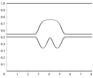
Physical regimes for which mode-2 internal solitary waves can be described by the MCC solutions are first identified. In the case when the thickness of the intermediate layer is much thinner than other layer thicknesses, it is then found that classical solitary wave profiles of large amplitude are difficult to compute. Using an asymptotic approach, it is shown that new classes of solutions to reduced equations in this limit, characterized by multi-humped profiles, exist at a countable, dense set of wave speeds. Previously, these multi-humped waves have been observed experimentally. For example, in the internal wave experiment of Gavrilov et al. (Reference Gavrilov, Liapidevskii and Liapidevskaya2013), a single hump on the upper interface over two humps on the lower interface was observed. Here, a rationale is presented to unveil a myriad of solutions obtained with different physical parameters.
This paper is organized as follows. The mathematical model for the three-layer system is introduced in § 2. After discussing in § 3 the weakly nonlinear limit of the model, we derive in § 4 the dynamical system governing its large amplitude solitary-wave solutions. The system is then investigated in § 5 within a few physical regimes for which asymptotic solutions are provided for the second baroclinic mode and compared with numerical solutions of the dynamical system. In § 6, for the case of thin transition layer with weak stratification, it is shown that multi-humped solitary waves are possible and their asymptotic and numerical solutions are presented. Concluding remarks are given in § 7.
2 Mathematical model
Consider a physical system composed of three homogeneous liquid layers with densities  $\unicode[STIX]{x1D70C}_{i}$,
  $i=1,2,3$ (from top to bottom), bounded above and below by rigid flat surfaces (see figure 1). To examine large amplitude long waves in this system, we adopt the strongly nonlinear multi-layer model proposed by Choi (Reference Choi, Goda, Ikehata and Suzuki2000), which, under weak horizontal vorticity and long wave (
 $\unicode[STIX]{x1D716}=H_{i}/\unicode[STIX]{x1D706}\ll 1$) assumptions, is formulated in terms of the thicknesses of each layer, denoted by
  $h_{i}$, and depth-averaged horizontal velocities
  $\overline{u}_{i}$. Namely, consisting of the mass conservation laws for each layer,
 $$\begin{eqnarray}h_{i,t}+(h_{i}\,\overline{u}_{i})_{x}=0,\end{eqnarray}$$
and the momentum equations,
 $$\begin{eqnarray}\overline{u}_{i,t}+\overline{u}_{i}\overline{u}_{i,x}+g\unicode[STIX]{x1D702}_{i,x}+\frac{P_{i,x}}{\unicode[STIX]{x1D70C}_{i}}=\frac{1}{h_{i}}\left(\frac{1}{3}h_{i}^{3}a_{i}+\frac{1}{2}h_{i}^{2}b_{i}\right)_{x}+\left(\frac{1}{2}h_{i}a_{i}+b_{i}\right)\unicode[STIX]{x1D702}_{i+1,x},\end{eqnarray}$$
 where  $a_{i}(x,t)=-(D_{i}^{2}h_{i})/h_{i}$ and
  $b_{i}(x,t)=-D_{i}^{2}\unicode[STIX]{x1D702}_{i+1}$ with
  $D_{i}=\unicode[STIX]{x2202}/\unicode[STIX]{x2202}t+\overline{u}_{i}\,\unicode[STIX]{x2202}/\unicode[STIX]{x2202}x$. The location of the upper and lower interfaces are defined by
  $z=\unicode[STIX]{x1D702}_{2}\equiv \unicode[STIX]{x1D701}_{1}(x,t)$ and
  $z=\unicode[STIX]{x1D702}_{3}\equiv -H_{2}+\unicode[STIX]{x1D701}_{2}(x,t)$, respectively. The two rigid walls are located at
  $z=\unicode[STIX]{x1D702}_{1}\equiv H_{1}$ and
  $z=\unicode[STIX]{x1D702}_{4}\equiv -(H_{2}+H_{3})$. The thickness of the
  $i$th layer
  $h_{i}$ is then given by
  $h_{i}=\unicode[STIX]{x1D702}_{i}-\unicode[STIX]{x1D702}_{i+1}$, or, more precisely,
 $$\begin{eqnarray}h_{1}=H_{1}-\unicode[STIX]{x1D701}_{1},\quad h_{2}=\unicode[STIX]{x1D701}_{1}-\unicode[STIX]{x1D701}_{2}+H_{2},\quad h_{3}=H_{3}+\unicode[STIX]{x1D701}_{2},\end{eqnarray}$$
 where  $H_{i}$ denotes the undisturbed thickness of the
  $i$th layer. The pressure at the location
  $z=\unicode[STIX]{x1D702}_{i}(x,t)$ denoted by
  $P_{i}$ satisfies the recursion formula
 $$\begin{eqnarray}P_{i+1}=P_{i}+\unicode[STIX]{x1D70C}_{i}(gh_{i}-{\textstyle \frac{1}{2}}a_{i}h_{i}^{2}-b_{i}h_{i}).\end{eqnarray}$$
 Therefore, for three-layer flows between two rigid walls, a closed system for nine unknowns  $h_{i}$,
  $\overline{u}_{i}$,
  $P_{i}$ (
 $i=1,2,3$) consists of (2.1) and (2.2) for
  $i=1,2,3$ and (2.4) for
  $i=1,2$ along with a geometric constraint given by
  $h_{1}+h_{2}+h_{3}=H_{1}+H_{2}+H_{3}$.

Figure 1. A three-fluid system.
Using (2.4), the momentum equations given by (2.2) can be also written as
 $$\begin{eqnarray}\overline{u}_{i,t}+\overline{u}_{i}\overline{u}_{i,x}+g\unicode[STIX]{x1D702}_{i+1,x}+\frac{P_{i+1,x}}{\unicode[STIX]{x1D70C}_{i}}=\frac{1}{h_{i}}\left(\frac{1}{3}{h_{i}}^{3}a_{i}-\frac{1}{2}{h_{i}}^{2}b_{i-1}\right)_{x}-\left(\frac{1}{2}h_{i}a_{i}-b_{i-1}\right)\unicode[STIX]{x1D702}_{i,x},\end{eqnarray}$$
 which might be more convenient for the top layer bounded above by a rigid wall, where the pressure is unknown. For two-layer flows between two rigid walls ( $\unicode[STIX]{x1D702}_{1,x}=\unicode[STIX]{x1D702}_{3,x}=0$), a system given by (2.5) for
  $i=1$, (2.2) for
  $i=2$, and (2.1) for
  $i=1,2$ yields the MCC equations.
These long wave models can be also given in conservative form, which is particularly well suited to examine their travelling-wave solutions. With this in view, equations (2.5) and (2.2) for the top ( $i=1$) and bottom (
 $i=3$) layers, respectively, are rewritten as
 $$\begin{eqnarray}\displaystyle & \displaystyle \left(\overline{u}_{1}+\frac{1}{6}h_{1}^{2}\,\overline{u}_{1,xx}\right)_{t}+\left(g\unicode[STIX]{x1D702}_{2}+\frac{1}{2}{\overline{u}_{1}}^{2}+\frac{1}{6}h_{1}^{2}\,\overline{u}_{1}\,\overline{u}_{1,xx}+\frac{P_{2}}{\unicode[STIX]{x1D70C}_{1}}+\frac{1}{2}h_{1}D_{1}^{2}\,h_{1}\right)_{x}=0, & \displaystyle\end{eqnarray}$$
 $$\begin{eqnarray}\displaystyle & \displaystyle \left(\overline{u}_{3}+\frac{1}{6}h_{3}^{2}\,\overline{u}_{3,xx}\right)_{t}+\left(g\unicode[STIX]{x1D702}_{3}+\frac{1}{2}{\overline{u}_{3}}^{2}+\frac{1}{6}h_{3}^{2}\,\overline{u}_{3}\,\overline{u}_{3,xx}+\frac{P_{3}}{\unicode[STIX]{x1D70C}_{3}}+\frac{1}{2}h_{3}D_{3}^{2}\,h_{3}\right)_{x}=0. & \displaystyle\end{eqnarray}$$
 For the intermediate layer ( $i=2$), the following two equivalent forms resulting from (2.2) and (2.5) will be useful:
 $$\begin{eqnarray}\displaystyle & \displaystyle U_{2,t}+(\overline{u}_{2}U_{2}+Q_{2})_{x}=0, & \displaystyle\end{eqnarray}$$
 $$\begin{eqnarray}\displaystyle & \displaystyle V_{2,t}+(\overline{u}_{2}V_{2}+R_{2})_{x}=0, & \displaystyle\end{eqnarray}$$
with
 $$\begin{eqnarray}\left.\begin{array}{@{}c@{}}\displaystyle U_{2}=\overline{u}_{2}+{\textstyle \frac{1}{6}}h_{2}^{2}\overline{u}_{2,xx}-{\textstyle \frac{1}{2}}h_{2}(D_{2}\unicode[STIX]{x1D702}_{3})_{x}+{\textstyle \frac{1}{2}}D_{2}h_{2}\,\unicode[STIX]{x1D702}_{3,x}+D_{2}\unicode[STIX]{x1D702}_{3}\,\unicode[STIX]{x1D702}_{3,x},\\ \displaystyle Q_{2}=-\frac{1}{2}\overline{u}_{2}^{2}+g\unicode[STIX]{x1D702}_{2}+\frac{P_{2}}{\unicode[STIX]{x1D70C}_{2}}+\frac{1}{2}h_{2}D_{2}^{2}h_{2}+h_{2}D_{2}^{2}\unicode[STIX]{x1D702}_{3}-\frac{1}{2}(D_{2}\unicode[STIX]{x1D702}_{3})^{2},\end{array}\right\}\end{eqnarray}$$
and
 $$\begin{eqnarray}\left.\begin{array}{@{}c@{}}\displaystyle V_{2}=\overline{u}_{2}+{\textstyle \frac{1}{6}}h_{2}^{2}\overline{u}_{2,xx}+{\textstyle \frac{1}{2}}h_{2}(D_{2}\unicode[STIX]{x1D702}_{2})_{x}-{\textstyle \frac{1}{2}}D_{2}h_{2}\,\unicode[STIX]{x1D702}_{2,x}+D_{2}\unicode[STIX]{x1D702}_{2}\,\unicode[STIX]{x1D702}_{2,x},\\ \displaystyle R_{2}=-\frac{1}{2}\overline{u}_{2}^{2}+g\unicode[STIX]{x1D702}_{3}+\frac{P_{3}}{\unicode[STIX]{x1D70C}_{2}}+\frac{1}{2}h_{2}D_{2}^{2}h_{2}-h_{2}D_{2}^{2}\unicode[STIX]{x1D702}_{2}-\frac{1}{2}(D_{2}\unicode[STIX]{x1D702}_{2})^{2}.\end{array}\right\}\end{eqnarray}$$
When convenient, it will be assumed, without loss of generality, that the stratification is given as
 $$\begin{eqnarray}\unicode[STIX]{x1D70C}_{1}=\unicode[STIX]{x1D70C}_{0}(1-\unicode[STIX]{x1D6E5}_{1}),\quad \unicode[STIX]{x1D70C}_{2}=\unicode[STIX]{x1D70C}_{0},\quad \unicode[STIX]{x1D70C}_{3}=\unicode[STIX]{x1D70C}_{0}(1+\unicode[STIX]{x1D6E5}_{2}),\end{eqnarray}$$
 with  $0<\unicode[STIX]{x1D6E5}_{1}<1$,
  $\unicode[STIX]{x1D6E5}_{2}>0$. Furthermore, we may introduce a parameter
  $\unicode[STIX]{x1D6FF}=\unicode[STIX]{x1D6E5}_{1}/\unicode[STIX]{x1D6E5}_{2}$ to write alternatively
  $\unicode[STIX]{x1D70C}_{1}=\unicode[STIX]{x1D70C}_{0}(1-\unicode[STIX]{x1D6FF}\unicode[STIX]{x1D6E5}_{2})$, with
  $0<\unicode[STIX]{x1D6FF}<1/\unicode[STIX]{x1D6E5}_{2}$.
When the system given by (2.1)–(2.2) is linearized about the equilibrium  $\unicode[STIX]{x1D701}_{1}=\unicode[STIX]{x1D701}_{2}=\overline{u}_{1}=\overline{u}_{2}=0$,
  $P_{1}=\text{const.}$, and solutions are sought as being proportional to
  $\exp [\text{i}k(x-ct)]$, with wavenumber
  $k$ and wave speed
  $c$, one obtains the linear dispersion relation for the model
 $$\begin{eqnarray}\displaystyle & & \displaystyle (\unicode[STIX]{x1D70C}_{1}\unicode[STIX]{x1D70C}_{2}H_{3}\unicode[STIX]{x1D703}_{1}\unicode[STIX]{x1D703}_{2}+\unicode[STIX]{x1D70C}_{1}\unicode[STIX]{x1D70C}_{3}H_{2}\unicode[STIX]{x1D703}_{1}\unicode[STIX]{x1D703}_{3}+\unicode[STIX]{x1D70C}_{2}^{2}H_{1}H_{2}H_{3}k^{2}\unicode[STIX]{x1D703}_{4}+\unicode[STIX]{x1D70C}_{2}\unicode[STIX]{x1D70C}_{3}H_{1}\unicode[STIX]{x1D703}_{2}\unicode[STIX]{x1D703}_{3})c^{4}\nonumber\\ \displaystyle & & \displaystyle \quad +\,g(\unicode[STIX]{x1D70C}_{1}(\unicode[STIX]{x1D70C}_{2}-\unicode[STIX]{x1D70C}_{3})H_{2}H_{3}\unicode[STIX]{x1D703}_{1}+\unicode[STIX]{x1D70C}_{2}(\unicode[STIX]{x1D70C}_{1}-\unicode[STIX]{x1D70C}_{3})H_{1}H_{3}\unicode[STIX]{x1D703}_{2}+\unicode[STIX]{x1D70C}_{3}(\unicode[STIX]{x1D70C}_{1}-\unicode[STIX]{x1D70C}_{2})H_{1}H_{2}\unicode[STIX]{x1D703}_{3})c^{2}\nonumber\\ \displaystyle & & \displaystyle \quad +\,g^{2}H_{1}H_{2}H_{3}(\unicode[STIX]{x1D70C}_{1}-\unicode[STIX]{x1D70C}_{2})(\unicode[STIX]{x1D70C}_{2}-\unicode[STIX]{x1D70C}_{3})=0,\end{eqnarray}$$
where
 $$\begin{eqnarray}\unicode[STIX]{x1D703}_{4}={\textstyle \frac{1}{12}}k^{2}H_{2}^{2}+1,\quad \unicode[STIX]{x1D703}_{i}={\textstyle \frac{1}{3}}k^{2}H_{i}^{2}+1,\quad i=1,2,3.\end{eqnarray}$$
Equation (2.13) yields two modes, known as mode 1 (faster) and mode 2 (slower) according to the magnitude of the wave speed (see figure 2). Notice that all four roots of (2.13) are always real, as shown in appendix A.
In the long-wave limit when  $k\rightarrow 0$, the linear long wave speeds
  $c_{0}^{\pm }$ are found as the roots of the equation
 $$\begin{eqnarray}\displaystyle & & \displaystyle (\unicode[STIX]{x1D70C}_{1}\unicode[STIX]{x1D70C}_{2}H_{3}+\unicode[STIX]{x1D70C}_{1}\unicode[STIX]{x1D70C}_{3}H_{2}+\unicode[STIX]{x1D70C}_{2}\unicode[STIX]{x1D70C}_{3}H_{1}){c_{0}}^{4}\nonumber\\ \displaystyle & & \displaystyle \quad +\,g(\unicode[STIX]{x1D70C}_{1}(\unicode[STIX]{x1D70C}_{2}-\unicode[STIX]{x1D70C}_{3})H_{2}H_{3}+\unicode[STIX]{x1D70C}_{2}(\unicode[STIX]{x1D70C}_{1}-\unicode[STIX]{x1D70C}_{3})H_{1}H_{3}+\unicode[STIX]{x1D70C}_{3}(\unicode[STIX]{x1D70C}_{1}-\unicode[STIX]{x1D70C}_{2})H_{1}H_{2}){c_{0}}^{2}\nonumber\\ \displaystyle & & \displaystyle \quad +\,g^{2}H_{1}H_{2}H_{3}(\unicode[STIX]{x1D70C}_{1}-\unicode[STIX]{x1D70C}_{2})(\unicode[STIX]{x1D70C}_{2}-\unicode[STIX]{x1D70C}_{3})=0.\end{eqnarray}$$
Furthermore, in the long-wave limit, it can be shown that the ratio between the two interface displacements is given by
 $$\begin{eqnarray}\frac{\unicode[STIX]{x1D701}_{2}}{\unicode[STIX]{x1D701}_{1}}=\frac{(\unicode[STIX]{x1D70C}_{1}H_{2}+\unicode[STIX]{x1D70C}_{2}H_{1})c_{0}^{2}-gH_{1}H_{2}(\unicode[STIX]{x1D70C}_{2}-\unicode[STIX]{x1D70C}_{1})}{\unicode[STIX]{x1D70C}_{2}H_{1}c_{0}^{2}}.\end{eqnarray}$$
This ratio can have different signs, according to the wave mode considered. Given that
 $$\begin{eqnarray}(c_{0}^{-})^{2}<\frac{gH_{1}H_{2}(\unicode[STIX]{x1D70C}_{2}-\unicode[STIX]{x1D70C}_{1})}{\unicode[STIX]{x1D70C}_{1}H_{2}+\unicode[STIX]{x1D70C}_{2}H_{1}}<(c_{0}^{+})^{2},\end{eqnarray}$$
it then follows from (2.16) that linear long waves of the second (first) baroclinic mode have the opposite (same) polarities.

Figure 2. Dispersion relation (2.13) for different physical parameters. The axes have been non-dimensionalized by the total depth  $H=H_{1}+H_{2}+H_{3}$, and the plots show how the square of the Froude number
  $c^{2}/gH$ depends on the dimensionless wavenumber
  $kH$. The dashed lines correspond to the linearized Euler equations and the solid lines correspond to the present model (2.1)–(2.2). The stratification is given by (2.12), with
  $\unicode[STIX]{x1D6E5}_{1}=\unicode[STIX]{x1D6FF}\unicode[STIX]{x1D6E5}_{2}$, and the physical parameters are set to
  $H_{1}/H=0.4$,
  $H_{2}/H=0.2$,
  $\unicode[STIX]{x1D6E5}_{2}=0.1$. (a)
  $\unicode[STIX]{x1D6FF}=1$, (b)
  $\unicode[STIX]{x1D6FF}=5$.
3 Weakly nonlinear theory
We show in this section that the strongly nonlinear model reduces, in the weakly nonlinear limit of  $a/H_{i}=O(H_{i}^{2}/\unicode[STIX]{x1D706}^{2})$, with
  $a$ and
  $\unicode[STIX]{x1D706}$ typical values of amplitude and wavelength, to Boussinesq-type equations. The weakly nonlinear model consists of (2.1) and
 $$\begin{eqnarray}\overline{u}_{i,t}+\overline{u}_{i}\overline{u}_{i,x}+g\unicode[STIX]{x1D702}_{i,x}+\frac{P_{i,x}}{\unicode[STIX]{x1D70C}_{i}}=+\frac{1}{3}H_{i}^{2}\,\overline{u}_{i,xxt}-\frac{1}{2}H_{i}\,\unicode[STIX]{x1D702}_{i+1,xtt},\end{eqnarray}$$
 where  $i=1$, 2, 3 and the pressure
  $P_{i}$ is given recursively by
 $$\begin{eqnarray}P_{i+1}=P_{i}+\unicode[STIX]{x1D70C}_{i}(gh_{i}-{\textstyle \frac{1}{2}}H_{i}^{2}\,\overline{u}_{i,xt}+H_{i}\,\unicode[STIX]{x1D702}_{i+1,tt}),\end{eqnarray}$$
 with  $\unicode[STIX]{x1D702}_{1,t}=0$,
  $\unicode[STIX]{x1D702}_{2,t}=\unicode[STIX]{x1D701}_{1,t}$,
  $\unicode[STIX]{x1D702}_{3,t}=\unicode[STIX]{x1D701}_{2,t}$ and
  $\unicode[STIX]{x1D702}_{4,t}=0$.
Furthermore, if only uni-directional waves are considered, a Korteweg–de Vries (KdV) model can be derived, for example, for the upper interface, as
 $$\begin{eqnarray}\unicode[STIX]{x1D701}_{1,t}+c_{0}\,\unicode[STIX]{x1D701}_{1,x}+\unicode[STIX]{x1D6FC}\,\unicode[STIX]{x1D701}_{1}\,\unicode[STIX]{x1D701}_{1,x}+\unicode[STIX]{x1D6FD}\,\unicode[STIX]{x1D701}_{1,xxx}=0,\end{eqnarray}$$
 with coefficients  $\unicode[STIX]{x1D6FC}$ and
  $\unicode[STIX]{x1D6FD}$ given by
 $$\begin{eqnarray}\left.\begin{array}{@{}c@{}}\displaystyle \unicode[STIX]{x1D6FC}=\frac{3}{2}c_{0}\frac{\displaystyle \frac{\unicode[STIX]{x1D70C}_{3}}{H_{3}^{2}}\unicode[STIX]{x1D6FE}^{3}+\frac{\unicode[STIX]{x1D70C}_{2}}{H_{2}^{2}}(1-\unicode[STIX]{x1D6FE})^{3}-\frac{\unicode[STIX]{x1D70C}_{1}}{H_{1}^{2}}}{\displaystyle \frac{\unicode[STIX]{x1D70C}_{3}}{H_{3}}\unicode[STIX]{x1D6FE}^{2}+\frac{\unicode[STIX]{x1D70C}_{2}}{H_{2}}(1-\unicode[STIX]{x1D6FE})^{2}+\frac{\unicode[STIX]{x1D70C}_{1}}{H_{1}}},\\ \displaystyle \unicode[STIX]{x1D6FD}=\frac{1}{6}c_{0}\frac{\unicode[STIX]{x1D70C}_{3}H_{3}\unicode[STIX]{x1D6FE}^{2}+\unicode[STIX]{x1D70C}_{2}H_{2}(1+\unicode[STIX]{x1D6FE}+\unicode[STIX]{x1D6FE}^{2})+\unicode[STIX]{x1D70C}_{1}H_{1}}{\displaystyle \frac{\unicode[STIX]{x1D70C}_{3}}{H_{3}}\unicode[STIX]{x1D6FE}^{2}+\frac{\unicode[STIX]{x1D70C}_{2}}{H_{2}}(1-\unicode[STIX]{x1D6FE})^{2}+\frac{\unicode[STIX]{x1D70C}_{1}}{H_{1}}},\end{array}\right\}\end{eqnarray}$$
 where  $\unicode[STIX]{x1D6FE}$ is defined as
 $$\begin{eqnarray}\unicode[STIX]{x1D6FE}=1+\frac{\unicode[STIX]{x1D70C}_{1}H_{2}}{\unicode[STIX]{x1D70C}_{2}H_{1}}-g\left(\frac{\unicode[STIX]{x1D70C}_{2}-\unicode[STIX]{x1D70C}_{1}}{\unicode[STIX]{x1D70C}_{2}}\right)\frac{H_{2}}{c_{0}^{2}},\end{eqnarray}$$
or, alternatively,
 $$\begin{eqnarray}\unicode[STIX]{x1D6FE}=\left[1+\frac{\unicode[STIX]{x1D70C}_{3}H_{2}}{\unicode[STIX]{x1D70C}_{2}H_{3}}-g\left(\frac{\unicode[STIX]{x1D70C}_{3}-\unicode[STIX]{x1D70C}_{2}}{\unicode[STIX]{x1D70C}_{2}}\right)\frac{H_{2}}{c_{0}^{2}}\right]^{-1}.\end{eqnarray}$$
Here we have used (2.15), which can be written as
 $$\begin{eqnarray}\left[1+\frac{\unicode[STIX]{x1D70C}_{1}H_{2}}{\unicode[STIX]{x1D70C}_{2}H_{1}}-g\left(\frac{\unicode[STIX]{x1D70C}_{2}-\unicode[STIX]{x1D70C}_{1}}{\unicode[STIX]{x1D70C}_{2}}\right)\frac{H_{2}}{c_{0}^{2}}\right]\left[1+\frac{\unicode[STIX]{x1D70C}_{3}H_{2}}{\unicode[STIX]{x1D70C}_{2}H_{3}}-g\left(\frac{\unicode[STIX]{x1D70C}_{3}-\unicode[STIX]{x1D70C}_{2}}{\unicode[STIX]{x1D70C}_{2}}\right)\frac{H_{2}}{c_{0}^{2}}\right]=1.\end{eqnarray}$$
 Then, the lower interface is determined through the relationship  $\unicode[STIX]{x1D701}_{2}=\unicode[STIX]{x1D6FE}\unicode[STIX]{x1D701}_{1}$, in agreement with linear theory (see (2.16)). First and second baroclinic mode solutions are obtained by considering
  $c_{0}^{+}$ and
  $c_{0}^{-}$, respectively, in the definition of
  $\unicode[STIX]{x1D6FE}$, which implies
  $\unicode[STIX]{x1D6FE}^{+}>0$ and
  $\unicode[STIX]{x1D6FE}^{-}<0$.
3.1 Boussinesq approximation
The Boussinesq approximation is commonly adopted in the study of stratified fluids when the density variation is small. For the physical system under consideration, under the Boussinesq approximation, both  $\unicode[STIX]{x1D6E5}_{1}=(\unicode[STIX]{x1D70C}_{2}-\unicode[STIX]{x1D70C}_{1})/\unicode[STIX]{x1D70C}_{2}$ and
  $\unicode[STIX]{x1D6E5}_{2}=(\unicode[STIX]{x1D70C}_{3}-\unicode[STIX]{x1D70C}_{2})/\unicode[STIX]{x1D70C}_{2}$ are assumed small (
 $\ll 1$) and of the same order of magnitude. Then, the coefficients of the KdV equation (3.3) are simplified to
 $$\begin{eqnarray}\left.\begin{array}{@{}c@{}}\displaystyle \unicode[STIX]{x1D6FC}=\frac{3}{2}c_{0}\frac{\displaystyle \frac{1}{H_{3}^{2}}\unicode[STIX]{x1D6FE}^{3}+\frac{1}{H_{2}^{2}}(1-\unicode[STIX]{x1D6FE})^{3}-\frac{1}{H_{1}^{2}}}{\displaystyle \frac{1}{H_{3}}\unicode[STIX]{x1D6FE}^{2}+\frac{1}{H_{2}}(1-\unicode[STIX]{x1D6FE})^{2}+\frac{1}{H_{1}}},\\ \displaystyle \unicode[STIX]{x1D6FD}=\frac{1}{6}c_{0}\frac{H_{3}\unicode[STIX]{x1D6FE}^{2}+H_{2}(1+\unicode[STIX]{x1D6FE}+\unicode[STIX]{x1D6FE}^{2})+H_{1}}{\displaystyle \frac{1}{H_{3}}\unicode[STIX]{x1D6FE}^{2}+\frac{1}{H_{2}}(1-\unicode[STIX]{x1D6FE})^{2}+\frac{1}{H_{1}}},\end{array}\right\}\end{eqnarray}$$
 with  $\unicode[STIX]{x1D6FE}$ now given by
 $$\begin{eqnarray}\unicode[STIX]{x1D6FE}=1+\frac{H_{2}}{H_{1}}-\frac{g_{1}^{\prime }H_{2}}{c_{0}^{2}},\end{eqnarray}$$
or, equivalently,
 $$\begin{eqnarray}\unicode[STIX]{x1D6FE}=\left[1+\frac{H_{2}}{H_{3}}-\frac{g_{2}^{\prime }H_{2}}{c_{0}^{2}}\right]^{-1},\end{eqnarray}$$
 in order to satisfy the condition for the linear long wave speeds. Here,  $g_{1}^{\prime }=g\unicode[STIX]{x1D6E5}_{1}$ and
  $g_{2}^{\prime }=g\unicode[STIX]{x1D6E5}_{2}$ denote reduced gravities. These coefficients coincide with those presented by Yang et al. (Reference Yang, Fang, Tang and Ramp2010), based on the work by Benney (Reference Benney1966) (see also Benjamin Reference Benjamin1966; Grimshaw Reference Grimshaw1981).
3.2 Criticality condition and polarity of internal solitary waves
Based on KdV theory for (3.3), solitary-wave solutions may have different polarities, according to the sign of the quadratic nonlinearity coefficient  $\unicode[STIX]{x1D6FC}$ (notice that
  $\unicode[STIX]{x1D6FD}>0$), being of elevation (depression) when
  $\unicode[STIX]{x1D6FC}>0$ (
 ${<}0$). The KdV model also predicts that no solitary-wave solutions exist in the critical case when the quadratic nonlinearity coefficient vanishes, i.e.
 $$\begin{eqnarray}\frac{\unicode[STIX]{x1D70C}_{3}}{H_{3}^{2}}\unicode[STIX]{x1D6FE}^{3}+\frac{\unicode[STIX]{x1D70C}_{2}}{H_{2}^{2}}(1-\unicode[STIX]{x1D6FE})^{3}-\frac{\unicode[STIX]{x1D70C}_{1}}{H_{1}^{2}}=0,\end{eqnarray}$$
 with  $\unicode[STIX]{x1D6FE}$ defined by (3.5). Figures 3 and 4 display how the criticality condition (3.11) depends on the physical parameters considered (similar diagrams can be found in Kurkina et al. (Reference Kurkina, Kurkin, Rouvinskaya and Soomere2006) and Yuan, Grimshaw & Johnson (Reference Yuan, Grimshaw and Johnson2018), under the Boussinesq approximation). It must be stressed that, contrary to the two-layer case (with or without a top rigid lid, cf. Choi & Camassa (Reference Choi and Camassa1999) and Barros (Reference Barros2016)), criticality cannot be expressed in a polynomial fashion on the physical parameters for each one of the wave modes considered (see appendix B for further considerations).

Figure 3. Criticality condition (3.11) for the slow mode (solid line). The shaded region represents the set of parameters for which the left-hand side of (3.11) is positive (i.e.  $\unicode[STIX]{x1D6FC}(\unicode[STIX]{x1D6FE}^{-})>0$), and, therefore, KdV theory predicts convex mode-2 waves. The axes have been non-dimensionalized by the total depth
  $H=H_{1}+H_{2}+H_{3}$ and the diagrams are presented on the
  $(H_{1}/H,H_{2}/H)$-plane. The stratification is given by (2.12), with
  $\unicode[STIX]{x1D6E5}_{1}=\unicode[STIX]{x1D6FF}\unicode[STIX]{x1D6E5}_{2}$, and
  $\unicode[STIX]{x1D6E5}_{2}=0.01$. (a)
  $\unicode[STIX]{x1D6FF}=0.5$, (b)
  $\unicode[STIX]{x1D6FF}=1$, (c)
  $\unicode[STIX]{x1D6FF}=2$.

Figure 4. Criticality condition (3.11) for the fast mode (solid line). The shaded region represents the set of parameters for which the left-hand side of (3.11) is positive (i.e.  $\unicode[STIX]{x1D6FC}(\unicode[STIX]{x1D6FE}^{+})>0$), and, therefore, KdV theory predicts mode-1 waves of elevation. The axes have been non-dimensionalized by the total depth
  $H=H_{1}+H_{2}+H_{3}$ and the diagrams are presented on the
  $(H_{1}/H,H_{2}/H)$-plane. The stratification is given by (2.12), with
  $\unicode[STIX]{x1D6E5}_{1}=\unicode[STIX]{x1D6FF}\unicode[STIX]{x1D6E5}_{2}$, and
  $\unicode[STIX]{x1D6E5}_{2}=0.01$. (a)
  $\unicode[STIX]{x1D6FF}=0.5$, (b)
  $\unicode[STIX]{x1D6FF}=1$, (c)
  $\unicode[STIX]{x1D6FF}=2$.
4 Formulation of solitary waves as a dynamical system
To examine the travelling-wave solutions of our model, we consider the ansatz  $\unicode[STIX]{x1D701}_{i}=\unicode[STIX]{x1D701}_{i}(X)$,
  $\overline{u}_{i}=\overline{u}_{i}(X)$ and
  $P_{1}=P_{1}(X)$, where
  $X=x-ct$. It follows from (2.1) that
 $$\begin{eqnarray}(\overline{u}_{i}-c)h_{i}=\text{const.}\equiv m_{i},\quad i=1,2,3.\end{eqnarray}$$
 We proceed by integrating once equations (2.6) and (2.8) and eliminating  $P_{2}$ to obtain
 $$\begin{eqnarray}\displaystyle & & \displaystyle {\textstyle \frac{1}{3}}h_{1}h_{2}(\unicode[STIX]{x1D70C}_{1}m_{1}^{2}h_{2}+\unicode[STIX]{x1D70C}_{2}m_{2}^{2}h_{1})\unicode[STIX]{x1D701}_{1}^{\prime \prime }+({\textstyle \frac{1}{6}}\unicode[STIX]{x1D70C}_{2}m_{2}^{2}h_{1}^{2}h_{2})\unicode[STIX]{x1D701}_{2}^{\prime \prime }\nonumber\\ \displaystyle & & \displaystyle \qquad +\,{\textstyle \frac{1}{6}}(\unicode[STIX]{x1D70C}_{1}m_{1}^{2}h_{2}^{2}-\unicode[STIX]{x1D70C}_{2}m_{2}^{2}h_{1}^{2})\unicode[STIX]{x1D701}_{1}^{\prime 2}+{\textstyle \frac{1}{3}}\unicode[STIX]{x1D70C}_{2}m_{2}^{2}h_{1}^{2}\,\unicode[STIX]{x1D701}_{1}^{\prime }\unicode[STIX]{x1D701}_{2}^{\prime }+{\textstyle \frac{1}{3}}\unicode[STIX]{x1D70C}_{2}m_{2}^{2}h_{1}^{2}\,\unicode[STIX]{x1D701}_{2}^{\prime 2}\nonumber\\ \displaystyle & & \displaystyle \quad =(\unicode[STIX]{x1D70C}_{2}\unicode[STIX]{x1D705}_{2}-\unicode[STIX]{x1D70C}_{1}\unicode[STIX]{x1D705}_{1})h_{1}^{2}h_{2}^{2}+{\textstyle \frac{1}{2}}\unicode[STIX]{x1D70C}_{1}m_{1}^{2}h_{2}^{2}-{\textstyle \frac{1}{2}}\unicode[STIX]{x1D70C}_{2}m_{2}^{2}h_{1}^{2}+(\unicode[STIX]{x1D70C}_{1}-\unicode[STIX]{x1D70C}_{2})g\unicode[STIX]{x1D702}_{2}h_{1}^{2}h_{2}^{2}.\end{eqnarray}$$
 Similarly, we integrate once equations (2.7) and (2.9) and eliminate  $P_{3}$, to yield
 $$\begin{eqnarray}\displaystyle & & \displaystyle {\textstyle \frac{1}{6}}\unicode[STIX]{x1D70C}_{2}m_{2}^{2}h_{2}h_{3}^{2}\,\unicode[STIX]{x1D701}_{1}^{\prime \prime }+{\textstyle \frac{1}{3}}(\unicode[STIX]{x1D70C}_{3}m_{3}^{2}h_{2}^{2}h_{3}+\unicode[STIX]{x1D70C}_{2}m_{2}^{2}h_{2}h_{3}^{2})\unicode[STIX]{x1D701}_{2}^{\prime \prime }\nonumber\\ \displaystyle & & \displaystyle \qquad -\,{\textstyle \frac{1}{3}}\unicode[STIX]{x1D70C}_{2}m_{2}^{2}h_{3}^{2}\,\unicode[STIX]{x1D701}_{1}^{\prime 2}-{\textstyle \frac{1}{3}}\unicode[STIX]{x1D70C}_{2}m_{2}^{2}h_{3}^{2}\,\unicode[STIX]{x1D701}_{1}^{\prime }\unicode[STIX]{x1D701}_{2}^{\prime }+{\textstyle \frac{1}{6}}(\unicode[STIX]{x1D70C}_{2}m_{2}^{2}h_{3}^{2}-\unicode[STIX]{x1D70C}_{3}m_{3}^{2}h_{2}^{2})\unicode[STIX]{x1D701}_{2}^{\prime 2}\nonumber\\ \displaystyle & & \displaystyle \quad =(\unicode[STIX]{x1D70C}_{3}\unicode[STIX]{x1D705}_{3}-\unicode[STIX]{x1D70C}_{2}\unicode[STIX]{x1D705}_{4})h_{2}^{2}h_{3}^{2}+{\textstyle \frac{1}{2}}\unicode[STIX]{x1D70C}_{2}m_{2}^{2}h_{3}^{2}-{\textstyle \frac{1}{2}}\unicode[STIX]{x1D70C}_{3}m_{3}^{2}h_{2}^{2}+(\unicode[STIX]{x1D70C}_{2}-\unicode[STIX]{x1D70C}_{3})g\unicode[STIX]{x1D702}_{3}h_{2}^{2}h_{3}^{2}.\end{eqnarray}$$
 Here, the constants  $\unicode[STIX]{x1D705}_{i}$,
  $i=1,2,3,4$ are simply integration constants, and thus can be determined by imposing boundary conditions. In particular, to study solitary-wave solutions, we impose the boundary conditions:
  $\unicode[STIX]{x1D701}_{i}$,
  $\unicode[STIX]{x1D701}_{i}^{\prime }$,
  $\unicode[STIX]{x1D701}_{i}^{\prime \prime }\rightarrow 0$,
  $\overline{u}_{i}\rightarrow 0$,
  $P_{1}\rightarrow P_{1}^{\infty }$, as
  $X$ goes to infinity, from which it follows that
  $m_{i}=-cH_{i}$, and
 $$\begin{eqnarray}\left.\begin{array}{@{}c@{}}\displaystyle \unicode[STIX]{x1D705}_{1}=\frac{1}{2}c^{2}+\frac{P_{2}^{\infty }}{\unicode[STIX]{x1D70C}_{1}},\quad \unicode[STIX]{x1D705}_{2}=\frac{1}{2}c^{2}+\frac{P_{2}^{\infty }}{\unicode[STIX]{x1D70C}_{2}},\quad \unicode[STIX]{x1D705}_{3}=\frac{1}{2}c^{2}-gH_{2}+\frac{P_{3}^{\infty }}{\unicode[STIX]{x1D70C}_{3}},\\ \displaystyle \unicode[STIX]{x1D705}_{4}=\frac{1}{2}c^{2}-gH_{2}+\frac{P_{3}^{\infty }}{\unicode[STIX]{x1D70C}_{2}}.\end{array}\right\}\end{eqnarray}$$
After rearrangement we can cast the dynamical system into the following form:
 $$\begin{eqnarray}\displaystyle & & \displaystyle c^{2}\left\{\frac{1}{3}\left(\unicode[STIX]{x1D70C}_{1}\frac{H_{1}^{2}}{h_{1}}+\unicode[STIX]{x1D70C}_{2}\frac{H_{2}^{2}}{h_{2}}\right)\unicode[STIX]{x1D701}_{1}^{\prime \prime }+\frac{1}{6}\unicode[STIX]{x1D70C}_{2}\frac{H_{2}^{2}}{h_{2}}\,\unicode[STIX]{x1D701}_{2}^{\prime \prime }+\frac{1}{6}\left(\unicode[STIX]{x1D70C}_{1}\frac{H_{1}^{2}}{h_{1}^{2}}-\unicode[STIX]{x1D70C}_{2}\frac{H_{2}^{2}}{h_{2}^{2}}\right)\unicode[STIX]{x1D701}_{1}^{\prime 2}+\frac{1}{3}\unicode[STIX]{x1D70C}_{2}\frac{H_{2}^{2}}{h_{2}^{2}}\,\unicode[STIX]{x1D701}_{1}^{\prime }\unicode[STIX]{x1D701}_{2}^{\prime }\right.\nonumber\\ \displaystyle & & \displaystyle \quad +\left.\frac{1}{3}\unicode[STIX]{x1D70C}_{2}\frac{H_{2}^{2}}{h_{2}^{2}}\,\unicode[STIX]{x1D701}_{2}^{\prime 2}\right\}=\frac{1}{2}c^{2}\left[(\unicode[STIX]{x1D70C}_{2}-\unicode[STIX]{x1D70C}_{1})+\unicode[STIX]{x1D70C}_{1}\frac{H_{1}^{2}}{h_{1}^{2}}-\unicode[STIX]{x1D70C}_{2}\frac{H_{2}^{2}}{h_{2}^{2}}\right]-g(\unicode[STIX]{x1D70C}_{2}-\unicode[STIX]{x1D70C}_{1})\unicode[STIX]{x1D701}_{1},\end{eqnarray}$$
 $$\begin{eqnarray}\displaystyle & & \displaystyle c^{2}\left\{\frac{1}{6}\unicode[STIX]{x1D70C}_{2}\frac{H_{2}^{2}}{h_{2}}\,\unicode[STIX]{x1D701}_{1}^{\prime \prime }+\frac{1}{3}\left(\unicode[STIX]{x1D70C}_{2}\frac{H_{2}^{2}}{h_{2}}+\unicode[STIX]{x1D70C}_{3}\frac{H_{3}^{2}}{h_{3}}\right)\unicode[STIX]{x1D701}_{2}^{\prime \prime }-\frac{1}{3}\unicode[STIX]{x1D70C}_{2}\frac{H_{2}^{2}}{h_{2}^{2}}\,\unicode[STIX]{x1D701}_{1}^{\prime 2}-\frac{1}{3}\unicode[STIX]{x1D70C}_{2}\frac{H_{2}^{2}}{h_{2}^{2}}\,\unicode[STIX]{x1D701}_{1}^{\prime }\unicode[STIX]{x1D701}_{2}^{\prime }\right.\nonumber\\ \displaystyle & & \displaystyle \quad +\left.\frac{1}{6}\left(\unicode[STIX]{x1D70C}_{2}\frac{H_{2}^{2}}{h_{2}^{2}}-\unicode[STIX]{x1D70C}_{3}\frac{H_{3}^{2}}{h_{3}^{2}}\right)\unicode[STIX]{x1D701}_{2}^{\prime 2}\right\}=\frac{1}{2}c^{2}\left[(\unicode[STIX]{x1D70C}_{3}-\unicode[STIX]{x1D70C}_{2})+\unicode[STIX]{x1D70C}_{2}\frac{H_{2}^{2}}{h_{2}^{2}}-\unicode[STIX]{x1D70C}_{3}\frac{H_{3}^{2}}{h_{3}^{2}}\right]-g(\unicode[STIX]{x1D70C}_{3}-\unicode[STIX]{x1D70C}_{2})\unicode[STIX]{x1D701}_{2}.\qquad \nonumber\\ \displaystyle & & \displaystyle\end{eqnarray}$$
 We may then introduce a potential  $V(\unicode[STIX]{x1D701}_{1},\unicode[STIX]{x1D701}_{2})$
 $$\begin{eqnarray}\displaystyle V(\unicode[STIX]{x1D701}_{1},\unicode[STIX]{x1D701}_{2}) & = & \displaystyle -\frac{1}{2}c^{2}\left(\unicode[STIX]{x1D70C}_{2}-\unicode[STIX]{x1D70C}_{1}+\unicode[STIX]{x1D70C}_{1}\frac{H_{1}}{h_{1}}\right)\unicode[STIX]{x1D701}_{1}+\frac{1}{2}(\unicode[STIX]{x1D70C}_{2}-\unicode[STIX]{x1D70C}_{1})g\,\unicode[STIX]{x1D701}_{1}^{2}\nonumber\\ \displaystyle & & \displaystyle -\,\frac{1}{2}c^{2}\left(\unicode[STIX]{x1D70C}_{3}-\unicode[STIX]{x1D70C}_{2}-\unicode[STIX]{x1D70C}_{3}\frac{H_{3}}{h_{3}}\right)\,\unicode[STIX]{x1D701}_{2}+\frac{1}{2}(\unicode[STIX]{x1D70C}_{3}-\unicode[STIX]{x1D70C}_{2})g\,\unicode[STIX]{x1D701}_{2}^{2}\nonumber\\ \displaystyle & & \displaystyle -\,\frac{1}{2}c^{2}\unicode[STIX]{x1D70C}_{2}\frac{H_{2}}{h_{2}}(\unicode[STIX]{x1D701}_{2}-\unicode[STIX]{x1D701}_{1}),\end{eqnarray}$$
 and a Lagrangian  ${\mathcal{L}}$:
 $$\begin{eqnarray}\displaystyle {\mathcal{L}}(\unicode[STIX]{x1D701}_{1},\unicode[STIX]{x1D701}_{2},\unicode[STIX]{x1D701}_{1}^{\prime },\unicode[STIX]{x1D701}_{2}^{\prime }) & = & \displaystyle \frac{1}{6}c^{2}\left(\unicode[STIX]{x1D70C}_{1}\frac{H_{1}^{2}}{h_{1}}+\unicode[STIX]{x1D70C}_{2}\frac{H_{2}^{2}}{h_{2}}\right)\unicode[STIX]{x1D701}_{1}^{\prime 2}\nonumber\\ \displaystyle & & \displaystyle +\,\frac{1}{6}c^{2}\unicode[STIX]{x1D70C}_{2}\frac{H_{2}^{2}}{h_{2}}\,\unicode[STIX]{x1D701}_{1}^{\prime }\unicode[STIX]{x1D701}_{2}^{\prime }+\frac{1}{6}c^{2}\left(\unicode[STIX]{x1D70C}_{2}\frac{H_{2}^{2}}{h_{2}}+\unicode[STIX]{x1D70C}_{3}\frac{H_{3}^{2}}{h_{3}}\right)\unicode[STIX]{x1D701}_{2}^{\prime 2}-V(\unicode[STIX]{x1D701}_{1},\unicode[STIX]{x1D701}_{2}),\qquad\end{eqnarray}$$
such that (4.5)–(4.6) are simply the Euler–Lagrangian equations
 $$\begin{eqnarray}{\mathcal{L}}_{\unicode[STIX]{x1D701}_{i}}-\frac{\text{d}}{\text{d}X}({\mathcal{L}}_{\unicode[STIX]{x1D701}_{i}^{\prime }})=0,\quad i=1,2.\end{eqnarray}$$
 Alternatively, the dynamical system (4.9) can be written as a Hamiltonian system with two degrees of freedom. To do so, consider the symmetric matrix  ${\mathcal{M}}$:
 $$\begin{eqnarray}{\mathcal{M}}(\unicode[STIX]{x1D701}_{1},\unicode[STIX]{x1D701}_{2})=\left[\begin{array}{@{}cc@{}}\displaystyle \frac{1}{3}c^{2}\left(\unicode[STIX]{x1D70C}_{1}\frac{H_{1}^{2}}{h_{1}}+\unicode[STIX]{x1D70C}_{2}\frac{H_{2}^{2}}{h_{2}}\right) & \displaystyle \frac{1}{6}c^{2}\unicode[STIX]{x1D70C}_{2}\frac{H_{2}^{2}}{h_{2}}\\ \displaystyle \frac{1}{6}c^{2}\unicode[STIX]{x1D70C}_{2}\frac{H_{2}^{2}}{h_{2}} & \displaystyle \frac{1}{3}c^{2}\left(\unicode[STIX]{x1D70C}_{2}\frac{H_{2}^{2}}{h_{2}}+\unicode[STIX]{x1D70C}_{3}\frac{H_{3}^{2}}{h_{3}}\right)\end{array}\right],\end{eqnarray}$$
 such that  ${\mathcal{L}}$ can be given in compact form as
 $$\begin{eqnarray}{\mathcal{L}}={\textstyle \frac{1}{2}}\boldsymbol{q}^{\prime \,\text{T}}{\mathcal{M}}\,\boldsymbol{q}^{\prime }-V(\boldsymbol{q}),\end{eqnarray}$$
 with  $\boldsymbol{q}=(\unicode[STIX]{x1D701}_{1},\unicode[STIX]{x1D701}_{2})$. By defining
  $\boldsymbol{p}=\unicode[STIX]{x2202}{\mathcal{L}}/\unicode[STIX]{x2202}\boldsymbol{q}^{\prime }$, we can then introduce the Hamiltonian
 $$\begin{eqnarray}\mathbb{H}=\boldsymbol{p}\boldsymbol{\cdot }\boldsymbol{q}^{\prime }-{\mathcal{L}},\end{eqnarray}$$
 which can be given explicitly in terms of the variables  $(\boldsymbol{q},\boldsymbol{p})$ as
 $$\begin{eqnarray}\mathbb{H}={\textstyle \frac{1}{2}}\boldsymbol{p}^{\text{T}}{\mathcal{M}}^{-1}\boldsymbol{p}+V,\end{eqnarray}$$
 by noticing that  $(\unicode[STIX]{x1D701}_{1}^{\prime },\unicode[STIX]{x1D701}_{2}^{\prime })\longmapsto (p_{1},p_{2})$ is a change of variables. Here, we have used the symmetry of
  ${\mathcal{M}}$ to write
  $\boldsymbol{p}={\mathcal{M}}\,\boldsymbol{q}^{\prime }$, together with the fact that
  ${\mathcal{M}}$ is non-singular. Finally, Hamilton’s equations corresponding to (4.9) are given by
 $$\begin{eqnarray}\boldsymbol{q}^{\prime }=\frac{\unicode[STIX]{x2202}\mathbb{H}}{\unicode[STIX]{x2202}\boldsymbol{p}},\quad \boldsymbol{p}^{\prime }=-\frac{\unicode[STIX]{x2202}\mathbb{H}}{\unicode[STIX]{x2202}\boldsymbol{q}}.\end{eqnarray}$$
4.1 Linearization at the origin
Clearly, the origin is a critical point of the dynamical system composed by (4.5)–(4.6). When linearized about the origin, the system can be cast into matrix form
 $$\begin{eqnarray}A\unicode[STIX]{x1D73B}^{\prime \prime }+B\unicode[STIX]{x1D73B}=0,\end{eqnarray}$$
 by introducing  $\unicode[STIX]{x1D73B}=(\unicode[STIX]{x1D701}_{1},\unicode[STIX]{x1D701}_{2})$ and symmetric matrices
 $$\begin{eqnarray}\left.\begin{array}{@{}c@{}}\displaystyle A=c^{2}\left[\begin{array}{@{}cc@{}}\displaystyle {\textstyle \frac{1}{3}}(\unicode[STIX]{x1D70C}_{1}H_{1}+\unicode[STIX]{x1D70C}_{2}H_{2}) & \displaystyle {\textstyle \frac{1}{6}}\unicode[STIX]{x1D70C}_{2}H_{2}\\ \displaystyle {\textstyle \frac{1}{6}}\unicode[STIX]{x1D70C}_{2}H_{2} & \displaystyle {\textstyle \frac{1}{3}}(\unicode[STIX]{x1D70C}_{2}H_{2}+\unicode[STIX]{x1D70C}_{3}H_{3})\end{array}\right],\\ \displaystyle B=\left[\begin{array}{@{}cc@{}}\displaystyle g(\unicode[STIX]{x1D70C}_{2}-\unicode[STIX]{x1D70C}_{1})-\left(\frac{\unicode[STIX]{x1D70C}_{1}}{H_{1}}+\frac{\unicode[STIX]{x1D70C}_{2}}{H_{2}}\right)c^{2} & \displaystyle c^{2}\frac{\unicode[STIX]{x1D70C}_{2}}{H_{2}}\\ \displaystyle c^{2}\frac{\unicode[STIX]{x1D70C}_{2}}{H_{2}} & \displaystyle g(\unicode[STIX]{x1D70C}_{3}-\unicode[STIX]{x1D70C}_{2})-\left(\frac{\unicode[STIX]{x1D70C}_{2}}{H_{2}}+\frac{\unicode[STIX]{x1D70C}_{3}}{H_{3}}\right)c^{2}\end{array}\right].\end{array}\right\}\end{eqnarray}$$
 Looking for values of  $\unicode[STIX]{x1D706}$ for which there are solutions of (4.15) of the form
  $\unicode[STIX]{x1D73B}=\boldsymbol{c}\text{e}^{\unicode[STIX]{x1D706}X}$, with
  $\boldsymbol{c}$ a non-zero vector, is equivalent to finding the eigenvalues of the system, given by the solutions of
 $$\begin{eqnarray}\operatorname{det}(B+\unicode[STIX]{x1D706}^{2}A)=0.\end{eqnarray}$$
 Moreover, it can be easily checked that  $A$ is a positive definite matrix. A classical result from linear algebra asserts that
  $\unicode[STIX]{x1D706}^{2}$ is a real root of the equation
 $$\begin{eqnarray}a_{0}\unicode[STIX]{x1D706}^{4}+a_{2}\unicode[STIX]{x1D706}^{2}+a_{4}=0,\end{eqnarray}$$
 with  $a_{0}>0$ and
  $a_{4}=\operatorname{det}B$, which is just a multiple of the right-hand side of (2.15). Collision of eigenvalues can only occur at the origin, i.e. when
  $c=c_{0}^{\pm }$. Moreover, their nature will change with different values of the wave speed. It can be shown that: the origin is a centre–centre equilibrium in the range
  $]\!0,c_{0}^{-}\![$, i.e. one has four pure imaginary eigenvalues
$]\!0,c_{0}^{-}\ $\pm \text{i}\unicode[STIX]{x1D706}_{1},\pm i\unicode[STIX]{x1D706}_{2}$; the origin is a saddle–centre in the range
  $]\!c_{0}^{-},c_{0}^{+}\! [$, i.e. one has two real eigenvalues
  $\pm \unicode[STIX]{x1D706}_{3}$ and two pure imaginary eigenvalues
  $\pm \text{i}\unicode[STIX]{x1D706}_{4}$; the origin is a saddle–saddle in the range
  $]\!c_{0}^{+},\infty \![$, i.e. one has four real eigenvalues
$]\!c_{0}^{+},\infty \ $\pm \unicode[STIX]{x1D706}_{5},\pm \unicode[STIX]{x1D706}_{6}$, with
  $\unicode[STIX]{x1D706}_{i}$ all positive.
4.2 System reduction under Boussinesq approximation
The Hamiltonian structure is preserved under the Boussinesq approximation and the corresponding solitary-wave solutions are governed by the Euler–Lagrange equations for the following Lagrangian  $\widetilde{{\mathcal{L}}}$:
 $$\begin{eqnarray}\widetilde{{\mathcal{L}}}(\unicode[STIX]{x1D701}_{1},\unicode[STIX]{x1D701}_{2},\unicode[STIX]{x1D701}_{1}^{\prime },\unicode[STIX]{x1D701}_{2}^{\prime })=\frac{1}{6}c^{2}\left(\frac{H_{1}^{2}}{h_{1}}+\frac{H_{2}^{2}}{h_{2}}\right)\unicode[STIX]{x1D701}_{1}^{\prime 2}+\frac{1}{6}c^{2}\frac{H_{2}^{2}}{h_{2}}\,\unicode[STIX]{x1D701}_{1}^{\prime }\unicode[STIX]{x1D701}_{2}^{\prime }+\frac{1}{6}c^{2}\left(\frac{H_{2}^{2}}{h_{2}}+\frac{H_{3}^{2}}{h_{3}}\right)\unicode[STIX]{x1D701}_{2}^{\prime 2}-\widetilde{V}(\unicode[STIX]{x1D701}_{1},\unicode[STIX]{x1D701}_{2}),\end{eqnarray}$$
 with  $\widetilde{V}$ defined by
 $$\begin{eqnarray}\widetilde{V}(\unicode[STIX]{x1D701}_{1},\unicode[STIX]{x1D701}_{2})=\frac{1}{2}\left\{-c^{2}\left(\frac{H_{1}^{2}}{h_{1}}+\frac{H_{2}^{2}}{h_{2}}+\frac{H_{3}^{2}}{h_{3}}\right)+g_{1}^{\prime }\,\unicode[STIX]{x1D701}_{1}^{2}+g_{2}^{\prime }\,\unicode[STIX]{x1D701}_{2}^{2}+c^{2}(H_{1}+H_{2}+H_{3})\right\}.\end{eqnarray}$$
Furthermore, the dynamical system
 $$\begin{eqnarray}\widetilde{{\mathcal{L}}}_{\unicode[STIX]{x1D701}_{i}}-\frac{\text{d}}{\text{d}X}(\widetilde{{\mathcal{L}}}_{\unicode[STIX]{x1D701}_{i}^{\prime }})=0,\quad i=1,2,\end{eqnarray}$$
can be cast into the form
 $$\begin{eqnarray}T_{1}[\unicode[STIX]{x1D701}_{1},\unicode[STIX]{x1D701}_{2}]=0,\quad T_{2}[\unicode[STIX]{x1D701}_{1},\unicode[STIX]{x1D701}_{2}]=0,\end{eqnarray}$$
which correspond to a system of differential equations
 $$\begin{eqnarray}\displaystyle & & \displaystyle c^{2}\left\{\frac{1}{3}\left(\frac{H_{1}^{2}}{h_{1}}+\frac{H_{2}^{2}}{h_{2}}\right)\unicode[STIX]{x1D701}_{1}^{\prime \prime }+\frac{1}{6}\frac{H_{2}^{2}}{h_{2}}\,\unicode[STIX]{x1D701}_{2}^{\prime \prime }+\frac{1}{6}\left(\frac{H_{1}^{2}}{h_{1}^{2}}-\frac{H_{2}^{2}}{h_{2}^{2}}\right)\unicode[STIX]{x1D701}_{1}^{\prime 2}\right.\nonumber\\ \displaystyle & & \displaystyle \quad +\left.\frac{1}{3}\frac{H_{2}^{2}}{h_{2}^{2}}\,\unicode[STIX]{x1D701}_{1}^{\prime }\unicode[STIX]{x1D701}_{2}^{\prime }+\frac{1}{3}\frac{H_{2}^{2}}{h_{2}^{2}}\,\unicode[STIX]{x1D701}_{2}^{\prime 2}\right\}=\frac{1}{2}c^{2}\left(\frac{H_{1}^{2}}{h_{1}^{2}}-\frac{H_{2}^{2}}{h_{2}^{2}}\right)-g_{1}^{\prime }\unicode[STIX]{x1D701}_{1},\end{eqnarray}$$
 $$\begin{eqnarray}\displaystyle & & \displaystyle c^{2}\left\{\frac{1}{6}\frac{H_{2}^{2}}{h_{2}}\,\unicode[STIX]{x1D701}_{1}^{\prime \prime }+\frac{1}{3}\left(\frac{H_{2}^{2}}{h_{2}}+\frac{H_{3}^{2}}{h_{3}}\right)\unicode[STIX]{x1D701}_{2}^{\prime \prime }-\frac{1}{3}\frac{H_{2}^{2}}{h_{2}^{2}}\,\unicode[STIX]{x1D701}_{1}^{\prime 2}\right.\nonumber\\ \displaystyle & & \displaystyle \quad -\left.\frac{1}{3}\frac{H_{2}^{2}}{h_{2}^{2}}\,\unicode[STIX]{x1D701}_{1}^{\prime }\unicode[STIX]{x1D701}_{2}^{\prime }+\frac{1}{6}\left(\frac{H_{2}^{2}}{h_{2}^{2}}-\frac{H_{3}^{2}}{h_{3}^{2}}\right)\unicode[STIX]{x1D701}_{2}^{\prime 2}\right\}=\frac{1}{2}c^{2}\left(\frac{H_{2}^{2}}{h_{2}^{2}}-\frac{H_{3}^{2}}{h_{3}^{2}}\right)-g_{2}^{\prime }\unicode[STIX]{x1D701}_{2}.\end{eqnarray}$$
 We note here that the equations under the Boussinesq approximation are invariant under the transformation  $g\rightarrow -g$ and
  $\unicode[STIX]{x1D6E5}_{1}\rightarrow -\unicode[STIX]{x1D6E5}_{1},\unicode[STIX]{x1D6E5}_{2}\rightarrow -\unicode[STIX]{x1D6E5}_{2}$. Thus one may look at the interfaces ‘upside down’. Under this condition, for every solution pair
  $(\unicode[STIX]{x1D701}_{1},\unicode[STIX]{x1D701}_{2})$ of a given configuration with densities
  $\unicode[STIX]{x1D70C}_{0}(1-\unicode[STIX]{x1D6E5}_{1}),\unicode[STIX]{x1D70C}_{0},\unicode[STIX]{x1D70C}_{0}(1+\unicode[STIX]{x1D6E5}_{2})$ and undisturbed thickness of layers
  $H_{1}$,
  $H_{2}$,
  $H_{3}$ (from top to bottom),
  $(-\unicode[STIX]{x1D701}_{2},-\unicode[STIX]{x1D701}_{1})$ is a solution of the modified physical configuration with densities
  $\unicode[STIX]{x1D70C}_{0}(1-\unicode[STIX]{x1D6E5}_{2}),\unicode[STIX]{x1D70C}_{0},\unicode[STIX]{x1D70C}_{0}(1+\unicode[STIX]{x1D6E5}_{1})$, where the undisturbed thickness of layers are
  $H_{3}$,
  $H_{2}$,
  $H_{1}$ (from top to bottom).
5 Internal solitary-wave solutions of the second baroclinic mode
In this section, we first use asymptotics to find approximate solutions of (4.5)–(4.6) for large amplitude internal solitary waves of the slow (second baroclinic) mode under the assumption of weak density stratification. Then we confirm the asymptotic solutions with numerical solutions of (4.5)–(4.6).
It would be reasonable to expect that solitary-wave solutions of the first baroclinic mode in a three-layer flow can be approximated by those in a two-layer flow bounded by rigid boundaries, provided the thickness of the intermediate layer is thin enough (see appendix D). In a way, this would explain the success achieved by the MCC model in describing mode-1 solitary waves in salt-stratified laboratory experiments (Camassa et al. Reference Camassa, Choi, Michallet, Rusas and Sveen2006). What is perhaps surprising is that in certain regimes mode-2 waves in a three-layer flow can also be approximated by those in a two-layer flow by choosing layer thicknesses appropriately, as discussed below.
We start by writing the dynamical system (4.5)–(4.6) in non-dimensional variables as
 $$\begin{eqnarray}\displaystyle & & \displaystyle F^{2}\left\{\frac{1}{3}\left(\frac{\unicode[STIX]{x1D70E}_{1}}{h_{1}}+\frac{r_{2}^{2}}{h_{2}}\right)\unicode[STIX]{x1D701}_{1}^{\prime \prime }+\frac{1}{6}\frac{r_{2}^{2}}{h_{2}}\,\unicode[STIX]{x1D701}_{2}^{\prime \prime }+\frac{1}{6}\left(\frac{\unicode[STIX]{x1D70E}_{1}}{h_{1}^{2}}-\frac{r_{2}^{2}}{h_{2}^{2}}\right)\unicode[STIX]{x1D701}_{1}^{\prime 2}\right.\nonumber\\ \displaystyle & & \displaystyle \quad +\left.\frac{1}{3}\frac{r_{2}^{2}}{h_{2}^{2}}\,\unicode[STIX]{x1D701}_{1}^{\prime }\unicode[STIX]{x1D701}_{2}^{\prime }+\frac{1}{3}\frac{r_{2}^{2}}{h_{2}^{2}}\,\unicode[STIX]{x1D701}_{2}^{\prime 2}\right\}=\frac{1}{2}F^{2}\left[(1-\unicode[STIX]{x1D70E}_{1})+\frac{\unicode[STIX]{x1D70E}_{1}}{h_{1}^{2}}-\frac{r_{2}^{2}}{h_{2}^{2}}\right]-(1-\unicode[STIX]{x1D70E}_{1})\,\unicode[STIX]{x1D701}_{1},\end{eqnarray}$$
 $$\begin{eqnarray}\displaystyle & & \displaystyle F^{2}\left\{\frac{1}{6}\frac{r_{2}^{2}}{h_{2}}\,\unicode[STIX]{x1D701}_{1}^{\prime \prime }+\frac{1}{3}\left(\frac{r_{2}^{2}}{h_{2}}+\frac{\unicode[STIX]{x1D70E}_{3}\,r_{3}^{2}}{h_{3}}\right)\unicode[STIX]{x1D701}_{2}^{\prime \prime }-\frac{1}{3}\frac{r_{2}^{2}}{h_{2}^{2}}\,\unicode[STIX]{x1D701}_{1}^{\prime 2}-\frac{1}{3}\frac{r_{2}^{2}}{h_{2}^{2}}\,\unicode[STIX]{x1D701}_{1}^{\prime }\unicode[STIX]{x1D701}_{2}^{\prime }\right.\nonumber\\ \displaystyle & & \displaystyle \quad +\left.\frac{1}{6}\left(\frac{r_{2}^{2}}{h_{2}^{2}}-\frac{\unicode[STIX]{x1D70E}_{3}\,r_{3}^{2}}{h_{3}^{2}}\right)\unicode[STIX]{x1D701}_{2}^{\prime 2}\right\}=\frac{1}{2}F^{2}\left[(\unicode[STIX]{x1D70E}_{3}-1)+\frac{r_{2}^{2}}{h_{2}^{2}}-\frac{\unicode[STIX]{x1D70E}_{3}\,r_{3}^{2}}{h_{3}^{2}}\right]-(\unicode[STIX]{x1D70E}_{3}-1)\,\unicode[STIX]{x1D701}_{2}.\end{eqnarray}$$
 Here, we have introduced variables  $\unicode[STIX]{x1D701}_{i}^{\ast }=\unicode[STIX]{x1D701}_{i}/H_{1}$ and
  $h_{i}^{\ast }=h_{i}/H_{1}$. Derivatives are calculated with respect to
  $X^{\ast }=(x-ct)/H_{1}$ (as usual, the asterisks have been dropped for brevity), and the Froude number
  $F$, the density ratios
  $\unicode[STIX]{x1D70E}_{i}$
 $(i=1,3)$ and the depth ratios
  $r_{j}\;(j=2,3)$ are set as follows:
 $$\begin{eqnarray}F^{2}=c^{2}/gH_{1},\quad \unicode[STIX]{x1D70E}_{1}=\unicode[STIX]{x1D70C}_{1}/\unicode[STIX]{x1D70C}_{2},\quad \unicode[STIX]{x1D70E}_{3}=\unicode[STIX]{x1D70C}_{3}/\unicode[STIX]{x1D70C}_{2},\quad r_{2}=H_{2}/H_{1},\quad r_{3}=H_{3}/H_{1}.\end{eqnarray}$$
 Obviously, the system given by (5.1)–(5.2) has trivial solutions of  $\unicode[STIX]{x1D701}_{1}=\unicode[STIX]{x1D701}_{2}=0$ for which
  $h_{1}=1$,
  $h_{2}=r_{2}$, and
  $h_{3}=r_{3}$. Hereafter we focus on non-trivial solitary-wave solutions of the slow (second baroclinic) mode for the following three cases relevant for realistic oceanic conditions and some laboratory experiments:
(i) small density difference between two adjacent layers:
 $\unicode[STIX]{x1D70E}_{1}\simeq 1$, $\unicode[STIX]{x1D70E}_{3}-1=O(1)$;
(ii) small density differences across all three layers:
$\unicode[STIX]{x1D70E}_{1}\simeq 1$ and $\unicode[STIX]{x1D70E}_{3}\simeq 1$; and(iii) thin transition layer with weak stratification:
$\unicode[STIX]{x1D70E}_{1}\simeq 1$, $\unicode[STIX]{x1D70E}_{3}\simeq 1$, $r_{2}\ll 1$.


5.1 Case (i): small density difference between two adjacent layers
In this case, as  $1-\unicode[STIX]{x1D70E}_{1}\ll 1$, or
  $\unicode[STIX]{x1D6E5}_{1}\equiv 1-\unicode[STIX]{x1D70E}_{1}\ll 1$, the top and middle layers have nearly identical densities. Then the long wave speeds can be approximated, from (2.15), by
 $$\begin{eqnarray}\displaystyle & \displaystyle (c_{0}^{+})^{2}=\frac{g(\unicode[STIX]{x1D70C}_{3}-\unicode[STIX]{x1D70C}_{2})H_{3}(H_{1}+H_{2})}{\unicode[STIX]{x1D70C}_{2}H_{3}+\unicode[STIX]{x1D70C}_{3}(H_{1}+H_{2})}[1+O(\unicode[STIX]{x1D6E5}_{1})], & \displaystyle\end{eqnarray}$$
 $$\begin{eqnarray}\displaystyle & \displaystyle (c_{0}^{-})^{2}=\frac{gH_{1}H_{2}}{H_{1}+H_{2}}\left[\unicode[STIX]{x1D6E5}_{1}+\frac{H_{2}(H_{1}+H_{2})(\unicode[STIX]{x1D70C}_{3}-\unicode[STIX]{x1D70C}_{2})-\unicode[STIX]{x1D70C}_{2}H_{1}^{2}}{(H_{1}+H_{2})^{2}(\unicode[STIX]{x1D70C}_{3}-\unicode[STIX]{x1D70C}_{2})}\,\unicode[STIX]{x1D6E5}_{1}^{2}+O(\unicode[STIX]{x1D6E5}_{1}^{3})\right]. & \displaystyle\end{eqnarray}$$
This being the case, the displacement ratios for the two wave modes can be approximated, from (2.16), by
 $$\begin{eqnarray}\left(\frac{\unicode[STIX]{x1D701}_{2}}{\unicode[STIX]{x1D701}_{1}}\right)^{+}=\frac{H_{1}+H_{2}}{H_{1}}+O(\unicode[STIX]{x1D6E5}_{1}),\quad \left(\frac{\unicode[STIX]{x1D701}_{2}}{\unicode[STIX]{x1D701}_{1}}\right)^{-}=-\frac{\unicode[STIX]{x1D70C}_{2}H_{1}}{(\unicode[STIX]{x1D70C}_{3}-\unicode[STIX]{x1D70C}_{2})(H_{1}+H_{2})}\,\unicode[STIX]{x1D6E5}_{1}+O(\unicode[STIX]{x1D6E5}_{1}^{2}).\end{eqnarray}$$
 As can be seen (5.4), the first baroclinic mode of a three-layer system in this limit is almost equivalent to that of a two-layer system, where the density and thickness are given, respectively, by  $\unicode[STIX]{x1D70C}_{2}$ and
  $H_{1}+H_{2}$ for the upper layer and
  $\unicode[STIX]{x1D70C}_{3}$ and
  $H_{3}$ for the lower layer.
For the second baroclinic mode, since  $(\unicode[STIX]{x1D701}_{2}/\unicode[STIX]{x1D701}_{1})^{-}=O(\unicode[STIX]{x1D6E5}_{1})$, the displacement of the lower interface can be neglected for
  $\unicode[STIX]{x1D6E5}_{1}\ll 1$, which implies that the second interface can be replaced by a rigid boundary for the second baroclinic mode. Therefore, once again, the second baroclinic mode of a three-layer system can be approximated by the internal wave mode of a two-layer system, whose density and thickness are given, respectively, by
  $\unicode[STIX]{x1D70C}_{1}$ and
  $H_{1}$ for the upper layer and
  $\unicode[STIX]{x1D70C}_{2}$ and
  $H_{2}$ for the lower layer. This observation is also valid for the nonlinear problem, as shown next.
After writing  $\unicode[STIX]{x1D70E}_{1}=1-\unicode[STIX]{x1D700}$ (or
  $\unicode[STIX]{x1D6E5}_{1}=\unicode[STIX]{x1D700}\ll 1$), we assume from (5.5) that
  $F^{2}=\unicode[STIX]{x1D700}\,C$ with
  $C=O(1)$ for the slow mode. We seek approximate solutions of (5.1)–(5.2) by inserting into this set of equations the following expansions of the interface displacements:
  $\unicode[STIX]{x1D701}_{k}=\unicode[STIX]{x1D701}_{k,0}+\unicode[STIX]{x1D700}\,\unicode[STIX]{x1D701}_{k,1}+O(\unicode[STIX]{x1D700}^{2}),\,(k=1,2)$. The same representation will be adopted for each layer thickness
  $h_{i}=h_{i,0}+\unicode[STIX]{x1D700}h_{i,1}+O(\unicode[STIX]{x1D700}^{2}),\,(i=1,2,3)$. At leading order, it immediately follows from (5.2) that
  $\unicode[STIX]{x1D701}_{2,0}=0$, as expected from (5.6). We then conclude from (5.1) that
  $\unicode[STIX]{x1D701}_{1,0}$ is governed by
 $$\begin{eqnarray}C\left\{\frac{1}{3}\left(\frac{1}{h_{1,0}}+\frac{r_{2}^{2}}{h_{2,0}}\right)\unicode[STIX]{x1D701}_{1,0}^{\prime \prime }+\frac{1}{6}\left(\frac{\unicode[STIX]{x1D70E}_{1}}{h_{1,0}^{2}}-\frac{r_{2}^{2}}{h_{2,0}^{2}}\right)\unicode[STIX]{x1D701}_{1,0}^{\prime 2}\right\}=\frac{1}{2}C\left(\frac{1}{h_{1,0}^{2}}-\frac{r_{2}^{2}}{h_{2,0}^{2}}\right)-\unicode[STIX]{x1D701}_{1,0}.\end{eqnarray}$$
 After integrating this once after multiplying an integrating factor, or, equivalently, setting to zero for homoclinic trajectories the Hamiltonian  $\mathbb{H}$ defined by (4.13) with
  $\unicode[STIX]{x1D701}_{2,0}=0$, it can be shown that
  $\unicode[STIX]{x1D701}_{1,0}$ is a solution of
 $$\begin{eqnarray}\unicode[STIX]{x1D701}_{1,0}^{\prime 2}=\frac{3}{C}\frac{\unicode[STIX]{x1D701}_{1,0}^{2}[\unicode[STIX]{x1D701}_{1,0}^{2}-(1-r_{2})\,\unicode[STIX]{x1D701}_{1,0}+C(1+r_{2})-r_{2}]}{(1+r_{2})[(1-r_{2})\unicode[STIX]{x1D701}_{1,0}+r_{2}]}.\end{eqnarray}$$
When converted back to dimensional variables, we find that the upper interface is approximated by the solution of the equation
 $$\begin{eqnarray}\unicode[STIX]{x1D701}_{1}^{\prime 2}=\frac{3}{c^{2}}\frac{\unicode[STIX]{x1D701}_{1}^{2}[c^{2}(H_{2}+\unicode[STIX]{x1D701}_{1})+c^{2}(H_{1}-\unicode[STIX]{x1D701}_{1})-g\unicode[STIX]{x1D700}(H_{1}-\unicode[STIX]{x1D701}_{1})(H_{2}+\unicode[STIX]{x1D701}_{1})]}{c^{2}H_{1}^{2}(H_{2}+\unicode[STIX]{x1D701}_{1})+c^{2}H_{2}^{2}(H_{1}-\unicode[STIX]{x1D701}_{1})},\end{eqnarray}$$
 which is simply the MCC equation for the interface of two liquid layers confined by two rigid walls placed at  $z=H_{1}$ and
  $z=-H_{2}$, under the Boussinesq approximation. In this regime, we expect a large displacement of the interface
  $z=\unicode[STIX]{x1D701}_{1}(x,t)$ characterized by single-humped profile that broadens as the wave speed increases, while the displacement of the interface
  $z=-H_{2}+\unicode[STIX]{x1D701}_{2}(x,t)$ is almost imperceptible.
The reverse situation occurs when  $\unicode[STIX]{x1D70E}_{3}=1+\unicode[STIX]{x1D700}$ (
 $\unicode[STIX]{x1D700}\ll 1$) while
  $1-\unicode[STIX]{x1D70E}_{1}=O(1)$. The solutions of the second baroclinic mode are characterized by a large displacement of the lower interface
  $z=-H_{2}+\unicode[STIX]{x1D701}_{2}$, with an almost imperceptible displacement of the upper interface
  $z=\unicode[STIX]{x1D701}_{1}$.
5.2 Case (ii): small density difference across all three layers
When both density increments are small and of the same order so that  $\unicode[STIX]{x1D6E5}_{2}=O(\unicode[STIX]{x1D6E5}_{1})=O(\unicode[STIX]{x1D700})$, with
  $\unicode[STIX]{x1D700}\ll 1$, then the two linear long wave speeds become comparable and proportional to
  $\unicode[STIX]{x1D700}^{1/2}$, as can be seen from (5.4)–(5.5).
For simplicity, we consider the case when the density increments across the first and second interfaces are the same so that  $\unicode[STIX]{x1D70E}_{1}=1-\unicode[STIX]{x1D700}$ and
  $\unicode[STIX]{x1D70E}_{3}=1+\unicode[STIX]{x1D700}\;(\unicode[STIX]{x1D700}\ll 1)$. Therefore, we set
  $F^{2}=\unicode[STIX]{x1D700}\,C$ with
  $C=O(1)$ and let all other quantities be
  $O(1)$. As before, approximate solutions of (5.1)–(5.2) are sought by expanding the interface displacements in powers of
  $\unicode[STIX]{x1D700}$. Unfortunately, solving the leading-order system is as difficult as solving the full dynamical system. However, when the thicknesses of the top and bottom layers are almost the same (
 $r_{3}\approx 1$), some simplification can be made. As we will see, at leading order, mode-2 solutions are anti-symmetric and are governed by a Hamiltonian system with one degree of freedom.
To find such an approximate system, we assume the density increment across the layers is small and the same so that we can impose the Boussinesq approximation to the original system with  $g_{1}^{\prime }=g_{2}^{\prime }=g^{\prime }$. Furthermore, if the thicknesses of the unperturbed top and bottom layers are assumed the same so that
  $H_{1}=H_{3}$ (known as the symmetric configuration), the system (4.22) enjoys the following property:
 $$\begin{eqnarray}T_{2}[\unicode[STIX]{x1D701}_{1},\unicode[STIX]{x1D701}_{2}]=-T_{1}[-\unicode[STIX]{x1D701}_{2},-\unicode[STIX]{x1D701}_{1}].\end{eqnarray}$$
 This implies that, if  $(\unicode[STIX]{x1D701}_{1},\unicode[STIX]{x1D701}_{2})$ is a solution,
  $(-\unicode[STIX]{x1D701}_{2},-\unicode[STIX]{x1D701}_{1})$ is also a solution. In particular, anti-symmetric solutions of the form
  $\unicode[STIX]{x1D701}_{2}=-\unicode[STIX]{x1D701}_{1}$ are worth being considered, as the original system given by (4.5)–(4.6) or (5.1)–(5.2) can be reduced to a single equation. We remark that such constraint is in agreement with the predictions of the weakly nonlinear theory for the mode-2 ISW, given that the proportionality constant
  $\unicode[STIX]{x1D6FE}^{-}$ between the displacements of the two interfaces is simply
  $-1$, according to (3.9) with
  $(c_{0}^{-})^{2}=g^{\prime }H_{1}H_{2}/(2H_{1}+H_{2})$.
The anti-symmetric solutions can be found by solving the following leading-order equation, in dimensional variables, for  $\unicode[STIX]{x1D701}_{1}$:
 $$\begin{eqnarray}c^{2}\left\{\left(\frac{1}{3}\frac{H_{1}^{2}}{h_{1}}+\frac{1}{6}\frac{H_{2}^{2}}{h_{2}}\right)\unicode[STIX]{x1D701}_{1}^{\prime \prime }+\frac{1}{6}\left(\frac{H_{1}^{2}}{h_{1}^{2}}-\frac{H_{2}^{2}}{h_{2}^{2}}\right)\unicode[STIX]{x1D701}_{1}^{\prime 2}\right\}=\frac{1}{2}c^{2}\left(\frac{H_{1}^{2}}{h_{1}^{2}}-\frac{H_{2}^{2}}{h_{2}^{2}}\right)-g^{\prime }\unicode[STIX]{x1D701}_{1},\end{eqnarray}$$
which can be integrated once to yield the Hamiltonian
 $$\begin{eqnarray}\unicode[STIX]{x1D701}_{1}^{\prime 2}=\frac{6}{c^{2}}\frac{\unicode[STIX]{x1D701}_{1}^{2}[(2H_{1}+H_{2})c^{2}-g^{\prime }h_{1}h_{2}]}{2H_{1}^{2}h_{2}+H_{2}^{2}h_{1}},\end{eqnarray}$$
 where  $h_{1}=H_{1}-\unicode[STIX]{x1D701}_{1}$ and
  $h_{2}=2\unicode[STIX]{x1D701}_{1}+H_{2}$. This may be rewritten as
 $$\begin{eqnarray}\frac{1}{2}\unicode[STIX]{x1D701}_{1}^{\prime 2}=\left[\frac{6g^{\prime }}{(4H_{1}^{2}-H_{2}^{2})c^{2}}\right]\frac{\unicode[STIX]{x1D701}_{1}^{2}(\unicode[STIX]{x1D701}_{1}-a_{-})(\unicode[STIX]{x1D701}_{1}-a_{+})}{\unicode[STIX]{x1D701}_{1}-a_{\ast }}\equiv -K(\unicode[STIX]{x1D701}_{1}).\end{eqnarray}$$
 In (5.13),  $a_{\ast }$ is given by
 $$\begin{eqnarray}a_{\ast }=-\frac{H_{1}H_{2}}{2H_{1}-H_{2}},\end{eqnarray}$$
 and  $a_{\pm }$ are the two roots of a quadratic equation,
 $$\begin{eqnarray}\unicode[STIX]{x1D701}_{1}^{2}+q_{1}\unicode[STIX]{x1D701}_{1}+q_{2}=0,\end{eqnarray}$$
 with  $q_{1}$ and
  $q_{2}$ defined by
 $$\begin{eqnarray}q_{1}=-\frac{1}{2}(2H_{1}-H_{2}),\quad q_{2}=\frac{1}{2}H_{1}H_{2}\left(\frac{c^{2}}{(c_{0}^{-})^{2}}-1\right).\end{eqnarray}$$
 A homoclinic orbit for (5.13) is possible when  $K$ is negative through
  $\unicode[STIX]{x1D701}_{1}=0$ and
  $\unicode[STIX]{x1D701}_{1}=a_{\pm }$. For this to happen, the leading order of
  $K$ must be negative in a neighbourhood of the origin. We use Taylor series to expand
  $K$ around
  $\unicode[STIX]{x1D701}_{1}=0$ as
 $$\begin{eqnarray}K(\unicode[STIX]{x1D701}_{1})=-\frac{3g^{\prime }}{(2H_{1}+H_{2})c^{2}}\left(\frac{c^{2}}{(c_{0}^{-})^{2}}-1\right)\unicode[STIX]{x1D701}_{1}^{2}+O(\unicode[STIX]{x1D701}_{1}^{3}),\end{eqnarray}$$
 from which it follows that solitary waves exist only if  $c^{2}>(c_{0}^{-})^{2}$. Furthermore, when the roots
  $a_{\pm }$ coincide, the dynamical system admits a heteroclinic, rather than homoclinic, solution, connecting the origin
  $\unicode[STIX]{x1D701}_{1}=0$ to the critical point
  $\unicode[STIX]{x1D701}_{1}=a_{m}\equiv (2H_{1}-H_{2})/4$. This peculiar scenario occurs at the speed
  $c_{m}^{2}=g^{\prime }(2H_{1}+H_{2})/8$, and the corresponding solution is known as a front wave solution. Different wave polarities are possible depending on the sign of
  $2H_{1}-H_{2}$. More precisely, if
  $H_{2}<2H_{1}$, then
  $\unicode[STIX]{x1D701}_{1}(X)$ is a wave of elevation. Otherwise, it is a wave of depression. In the latter case, a curious feature holds: the value of
  $c_{m}$ can actually exceed the linear long wave speed
  $c_{0}^{+}$, provided
  $H_{2}>6H_{1}$. Such peculiar case will be further discussed in § 5.4 (see figure 16).

Figure 5. Anti-symmetric solutions governed by (5.13). These approximate the mode-2 solitary waves in a weakly stratified flow with the same density increment across the layers and nearly identical depths in equilibrium for the top and bottom layers. The upper and lower interfaces are plotted in dimensionless variables, i.e.  $\unicode[STIX]{x1D702}_{2}/H_{1}$ and
  $\unicode[STIX]{x1D702}_{3}/H_{1}$ are plotted as functions of
  $(x-ct)/H_{1}$. (a)
  $H_{2}/H_{1}=0.5$ and
  $a/H_{1}=0.1$,
  $0.3$,
  $0.374$. The corresponding wave speeds for
  $\unicode[STIX]{x1D6E5}_{1}=\unicode[STIX]{x1D6E5}_{2}=10^{-3}$ are
  $c^{2}/g^{\prime }H_{1}\approx 0.252,0.308,0.313$. (b)
  $H_{2}/H_{1}=5$ and
  $a/H_{1}=-0.1$,
  $-0.5$,
  $-0.74$. The corresponding wave speeds for
  $\unicode[STIX]{x1D6E5}_{1}=\unicode[STIX]{x1D6E5}_{2}=10^{-3}$ are
  $c^{2}/g^{\prime }H_{1}\approx 0.754,0.857,0.875$.
Equation (5.15) shows that the wave speed  $c$ can be written in terms of amplitude
  $a$ as
 $$\begin{eqnarray}\frac{c^{2}}{(c_{0}^{-})^{2}}=\frac{(H_{1}-a)(H_{2}+2a)}{H_{1}H_{2}},\end{eqnarray}$$
which can be convenient to plot the solutions of (5.13) as in figure 5.
Finally, and remarkably, the dynamical system obtained in this limit is precisely the same as in the MCC (two-layer) model, under the Boussinesq approximation, when the layers in equilibrium have thicknesses  $H_{1}$ and
  $H_{2}/2$ (see Gavrilov & Liapidevskii Reference Gavrilov and Liapidevskii2010).
5.3 Case (iii): thin transition layer with weak stratification
Another interesting limit is case (iii), where the middle layer is much thinner than the top and bottom layers, i.e.  $r_{2}\equiv H_{2}/H_{1}\ll 1$ while
  $H_{3}/H_{1}=O(1)$. In this case, the linear long wave speeds can be approximated by
 $$\begin{eqnarray}(c_{0}^{+})^{2}=\frac{g(\unicode[STIX]{x1D70C}_{3}-\unicode[STIX]{x1D70C}_{1})H_{1}H_{3}}{\unicode[STIX]{x1D70C}_{1}H_{3}+\unicode[STIX]{x1D70C}_{3}H_{1}}\left[1+O(r_{2})\right],\quad (c_{0}^{-})^{2}=\frac{g(\unicode[STIX]{x1D70C}_{2}-\unicode[STIX]{x1D70C}_{1})(\unicode[STIX]{x1D70C}_{3}-\unicode[STIX]{x1D70C}_{2})H_{1}}{\unicode[STIX]{x1D70C}_{2}(\unicode[STIX]{x1D70C}_{3}-\unicode[STIX]{x1D70C}_{1})}[r_{2}+O(r_{2}^{2})].\end{eqnarray}$$
Then, from (2.16), the displacement ratios for the two wave modes can be estimated as
 $$\begin{eqnarray}\left(\frac{\unicode[STIX]{x1D701}_{2}}{\unicode[STIX]{x1D701}_{1}}\right)^{+}=1+\frac{\unicode[STIX]{x1D70C}_{1}(\unicode[STIX]{x1D70C}_{3}-\unicode[STIX]{x1D70C}_{2})H_{3}+\unicode[STIX]{x1D70C}_{3}(\unicode[STIX]{x1D70C}_{1}-\unicode[STIX]{x1D70C}_{2})H_{1}}{\unicode[STIX]{x1D70C}_{2}(\unicode[STIX]{x1D70C}_{3}-\unicode[STIX]{x1D70C}_{1})H_{3}}\,r_{2}+O(r_{2}^{2}),\quad \left(\frac{\unicode[STIX]{x1D701}_{2}}{\unicode[STIX]{x1D701}_{1}}\right)^{-}=\frac{\unicode[STIX]{x1D70C}_{1}-\unicode[STIX]{x1D70C}_{2}}{\unicode[STIX]{x1D70C}_{3}-\unicode[STIX]{x1D70C}_{2}}+O(r_{2}).\end{eqnarray}$$
To find the solitary-wave solution of the first baroclinic mode, the thin middle layer can be neglected at leading order. Therefore, for the first baroclinic mode, the solitary-wave solutions of the three-layer system are expected to be in good agreement with those of the two-layer MCC model, as shown in appendix D. On the other hand, for the second baroclinic mode, more elaborate solutions can be found as discussed in the following.
Inspired by the work of Gavrilov et al. (Reference Gavrilov, Liapidevskii and Liapidevskaya2013), who first considered a variant of the strongly nonlinear multi-layer model (Choi Reference Choi, Goda, Ikehata and Suzuki2000) to study the propagation of mode-2 waves in a three-layer flow with a thin intermediate layer, we consider the case of a weakly stratified flow in which  $\unicode[STIX]{x1D70E}_{1}=1-\unicode[STIX]{x1D700}^{m}$ and
  $\unicode[STIX]{x1D70E}_{3}=1+\unicode[STIX]{x1D700}^{m}$, where
  $m$ is a positive integer and
  $\unicode[STIX]{x1D700}\ll 1$ measures the thickness of the thin intermediate layer, i.e.
  $r_{2}=O(\unicode[STIX]{x1D716})$. By applying the Boussinesq approximation to (5.19), the linear long wave speeds can be approximated as
 $$\begin{eqnarray}(c_{0}^{-})^{2}=\frac{1}{2}g^{\prime }H_{1}[r_{2}+O(r_{2}^{2})],\quad (c_{0}^{+})^{2}=\frac{2g^{\prime }H_{1}H_{3}}{H_{1}+H_{3}}[1+O(r_{2})],\end{eqnarray}$$
 where  $g^{\prime }=g\unicode[STIX]{x1D700}^{m}$. Therefore, regardless the value of
  $m$, one can see that the linear long wave speeds have the following orders of magnitude:
  $(c_{0}^{-})^{2}/gH_{1}=O(\unicode[STIX]{x1D700}^{1+m})$ and
  $(c_{0}^{+})^{2}/gH_{1}=O(\unicode[STIX]{x1D700}^{m})$.
Following the strategy employed for the previous cases, one would assume, from (5.19),  $F^{2}=O(\unicode[STIX]{x1D700}^{1+m})$ for mode-2 waves and seek asymptotic solutions to (5.1)–(5.2) by expanding the interface displacements in powers of
  $\unicode[STIX]{x1D700}$ as
  $\unicode[STIX]{x1D701}_{k}=\unicode[STIX]{x1D701}_{k,0}+\unicode[STIX]{x1D700}\,\unicode[STIX]{x1D701}_{k,1}+O(\unicode[STIX]{x1D700}^{2}),\,(k=1,2)$, while letting all other quantities to be
  $O(1)$. However, given that
  $\unicode[STIX]{x1D701}_{k,p}\equiv 0$ at any order
  $O(\unicode[STIX]{x1D716}^{p})$, this would yield the null solution. This implies that no finite amplitude solutions (
 $\unicode[STIX]{x1D701}_{k,0}\neq 0$) exist under the assumption of
  $F^{2}=O(\unicode[STIX]{x1D700}^{1+m})$. Note that this does not preclude the existence of solitary waves under the assumption of
  $\unicode[STIX]{x1D701}_{k}/H_{1}=O(r_{2})=O(\unicode[STIX]{x1D700})$, for a small range of wave speeds. For example, in the special case when
  $H_{3}=H_{1}$, anti-symmetric solutions can be found from (5.13) under the condition of
  $H_{2}/H_{1}\ll 1$.
One question that remains to be answered is if there exists any mode-2 solitary-wave solution of finite amplitude in a three-layer system with a thin transition layer so that  $\unicode[STIX]{x1D701}_{k,0}\neq 0$ although the solution might not be connected smoothly with small amplitude solutions. More specifically, we are looking for solutions whose amplitudes are comparable to
  $H_{1}$, which have been observed experimentally. To find such a solution, one might need to adopt a different approach, which will be further investigated in detail in § 6.
5.4 Numerical solutions
This section is not intended to address an exhaustive description of all possible internal solitary-wave solutions to the strongly nonlinear long wave model given by (4.5)–(4.6). Instead, we will focus on the second baroclinic mode for the cases of weak stratification, in particular, cases (i) and (ii), for which the asymptotic solutions have been obtained here.
After fixing the density ratios ( $\unicode[STIX]{x1D70C}_{1}/\unicode[STIX]{x1D70C}_{2}$ and
  $\unicode[STIX]{x1D70C}_{3}/\unicode[STIX]{x1D70C}_{2}$) and the depth ratios (
 $H_{2}/H_{1}$ and
  $H_{3}/H_{1}$), the wave profiles are calculated using a shooting method as in Barros & Gavrilyuk (Reference Barros and Gavrilyuk2007). Figure 6 illustrates solutions obtained for case (i), where the top and intermediate liquid layers have close density values (
 $\unicode[STIX]{x1D70C}_{1}/\unicode[STIX]{x1D70C}_{2}=0.9$), while a greater density difference is allowed for the bottom liquid layer (
 $\unicode[STIX]{x1D70C}_{3}/\unicode[STIX]{x1D70C}_{2}=2.0$). As expected from the asymptotic analysis in § 5.1, the deformation of the lower interface is almost imperceptible, while the displacement of the top interface is large and starts broadening as the wave speed increases.

Figure 6. Mode-2 internal solitary-wave solutions computed numerically for the dynamical system (4.5)–(4.6) for case (i). The upper and lower interfaces are plotted in dimensionless variables, i.e.  $\unicode[STIX]{x1D701}_{1}/H_{1}$ and
  $\unicode[STIX]{x1D701}_{2}/H_{1}$ are plotted as functions of
  $(x-ct)/H_{1}$. We set
  $\unicode[STIX]{x1D70C}_{1}/\unicode[STIX]{x1D70C}_{2}=0.9$,
  $\unicode[STIX]{x1D70C}_{3}/\unicode[STIX]{x1D70C}_{2}=2.0$,
  $H_{2}/H_{1}=0.5$,
  $H_{3}/H_{1}=1.0$ and consider different values for the wave speed. (a)
  $c^{2}/g_{1}^{\prime }H_{1}\approx 0.37$. (b)
  $c^{2}/g_{1}^{\prime }H_{1}\approx 0.387698$.
In figure 7, we consider case (ii), where the stratification is weak everywhere. Here we assume that the density increment across the layers is constant ( $\unicode[STIX]{x1D70C}_{1}/\unicode[STIX]{x1D70C}_{2}=0.999$,
  $\unicode[STIX]{x1D70C}_{3}/\unicode[STIX]{x1D70C}_{2}=1.001$) and, in equilibrium, the top and bottom layers have the same depth, or
  $H_{3}/H_{1}=1$. Because the Boussinesq approximation is not being imposed here, a slight break of symmetry of the dynamical system occurs. However, as predicted in § 5.2, solutions may still be well approximated by anti-symmetric solutions. Our numerical tests have revealed that when the intermediate layer is thick (
 $H_{2}/H_{1}=5$), solutions can be easily computed for any given wave speed. Waves with a single-hump profile seem to persist up to large values of the wave speed, and become broader as the wave speed increases, as shown in figure 7(a,b).
When the intermediate layer is thinner than the other two layers, e.g.  $H_{2}/H_{1}=0.5$, solutions with one single-hump profile become more difficult to compute. While we could find for
  $H_{2}/H_{1}=0.5$ asymptotic solutions with large amplitudes approaching a front, as shown in figure 5(a), we are able to find numerical solutions with wave amplitudes relatively smaller than the maximum amplitude predicted by the asymptotics. The solution presented in figure 7(c) is close to the largest amplitude wave solution we can compute with the current numerical method. It is not so clear if the solitary-wave solutions of the original system cease to exist at a smaller wave amplitude than the asymptotic prediction, or if an improved numerical method is required to larger amplitude waves of the original dynamical system with two degrees of freedom.
As the asymptotics in § 5.3 suggests, when the thickness of the middle layer decreases further, finding the large amplitude solitary-wave solutions of the original system given by (4.5)–(4.6) is a delicate subject. For this reason we reserve the following section for a detailed analysis for the case of a thin transition layer, complemented by numerics.

Figure 7. Mode-2 internal solitary-wave solutions computed numerically for the dynamical system (4.5)–(4.6) for case (ii) with  $H_{1}=H_{3}$. The upper and lower interfaces are plotted in dimensionless variables, i.e.
  $\unicode[STIX]{x1D701}_{1}/H_{1}$ and
  $\unicode[STIX]{x1D701}_{2}/H_{1}$ are plotted as functions of
  $(x-ct)/H_{1}$. In all cases we have set
  $\unicode[STIX]{x1D70C}_{1}/\unicode[STIX]{x1D70C}_{2}=0.999$,
  $\unicode[STIX]{x1D70C}_{3}/\unicode[STIX]{x1D70C}_{2}=1.001$,
  $H_{3}/H_{1}=1.0$. (a)
  $H_{2}/H_{1}=5$,
  $c^{2}/g^{\prime }H_{1}\approx 0.86$. (b)
  $H_{2}/H_{1}=5$,
  $c^{2}/g^{\prime }H_{1}\approx 0.874999$. (c)
  $H_{2}/H_{1}=0.5$,
  $c^{2}/g^{\prime }H_{1}\approx 0.281$.
6 Multi-humped internal solitary waves
6.1 Leading-order asymptotic solutions for a thin transition layer
Here we revisit case (iii) considered in § 5.3, where the thickness of the middle transition layer is assumed thin so that  $r_{2}=O(\unicode[STIX]{x1D700})$ with
  $\unicode[STIX]{x1D70E}_{1}=1-\unicode[STIX]{x1D700}^{m}$ and
  $\unicode[STIX]{x1D70E}_{3}=1+\unicode[STIX]{x1D700}^{m}$. When
  $F^{2}=\unicode[STIX]{x1D700}^{m}C$ is assumed (instead of
  $F^{2}=\unicode[STIX]{x1D700}^{m+1}C$) with
  $m$ positive integer and
  $C=O(1)$, the leading-order equations of (5.1)–(5.2) can be found, after dimensional variables are recovered, as
 $$\begin{eqnarray}\left.\begin{array}{@{}c@{}}\displaystyle (\unicode[STIX]{x1D701}_{1}-\unicode[STIX]{x1D701}_{2})^{2}\left\{2h_{1}\unicode[STIX]{x1D701}_{1}^{\prime \prime }+\unicode[STIX]{x1D701}_{1}^{\prime 2}-3+6g^{\prime }\frac{\unicode[STIX]{x1D701}_{1}h_{1}^{2}}{c^{2}H_{1}^{2}}\right\}=0,\\ \displaystyle (\unicode[STIX]{x1D701}_{1}-\unicode[STIX]{x1D701}_{2})^{2}\left\{2h_{3}\unicode[STIX]{x1D701}_{2}^{\prime \prime }-\unicode[STIX]{x1D701}_{2}^{\prime 2}+3+6g^{\prime }\frac{\unicode[STIX]{x1D701}_{2}h_{3}^{2}}{c^{2}H_{3}^{2}}\right\}=0,\end{array}\right\}\end{eqnarray}$$
 where  $H_{3}/H_{1}=O(1)$ and
  $\unicode[STIX]{x1D701}_{k}/H_{1}=O(1)$ (
 $k=1,2$) have been assumed. Notice that the same system can be obtained directly from (4.22) with
  $g_{1}^{\prime }=g_{2}^{\prime }=g^{\prime }$, and
  $H_{2}=0$. Therefore,
  $\unicode[STIX]{x1D701}_{1}=\unicode[STIX]{x1D701}_{2}$, or the following decoupled system of differential equations is satisfied:
 $$\begin{eqnarray}\displaystyle & \displaystyle 2h_{1}\unicode[STIX]{x1D701}_{1}^{\prime \prime }+\unicode[STIX]{x1D701}_{1}^{\prime 2}=3-6g^{\prime }\frac{\unicode[STIX]{x1D701}_{1}h_{1}^{2}}{c^{2}H_{1}^{2}}, & \displaystyle\end{eqnarray}$$
 $$\begin{eqnarray}\displaystyle & \displaystyle 2h_{3}\unicode[STIX]{x1D701}_{2}^{\prime \prime }-\unicode[STIX]{x1D701}_{2}^{\prime 2}=-3-6g^{\prime }\frac{\unicode[STIX]{x1D701}_{2}h_{3}^{2}}{c^{2}H_{3}^{2}}. & \displaystyle\end{eqnarray}$$
 Both equations can be solved analytically in terms of elliptic functions. We start with the first of these two equations. By multiplying both sides of (6.2) by  $h_{1}^{-1/2}$, one may integrate it once to have the following Hamiltonian:
 $$\begin{eqnarray}\frac{1}{2}\unicode[STIX]{x1D701}_{1}^{\prime 2}=\frac{3}{2c^{2}H_{1}^{2}}\unicode[STIX]{x1D701}_{1}(c^{2}H_{1}-g^{\prime }h_{1}\unicode[STIX]{x1D701}_{1}),\end{eqnarray}$$
which can be rewritten as
 $$\begin{eqnarray}\frac{1}{2}\unicode[STIX]{x1D701}_{1}^{\prime 2}=\frac{3g^{\prime }}{2c^{2}H_{1}^{2}}\unicode[STIX]{x1D701}_{1}(\unicode[STIX]{x1D701}_{1}-a_{-})(\unicode[STIX]{x1D701}_{1}-a_{+}),\end{eqnarray}$$
 where  $a_{\pm }$ are the roots of the equation
 $$\begin{eqnarray}\unicode[STIX]{x1D701}_{1}^{2}-H_{1}\unicode[STIX]{x1D701}_{1}+\frac{c^{2}H_{1}}{g^{\prime }}=0.\end{eqnarray}$$
 Notice that (6.5) can be also obtained from (5.13) with  $H_{2}=0$. Although no homoclinic orbits for solitary-wave solutions are possible, periodic orbits starting from rest at zero exist provided
  $c^{2}<(1/4)g^{\prime }H_{1}$, under which
  $a_{\pm }$ are real and positive. As shown later, when these (inner) solutions are connected to zero (outer) solutions, they will be the leading-order approximate solution to (5.1)–(5.2). When (6.5) is integrated once, one can obtain
 $$\begin{eqnarray}\frac{cH_{1}}{\sqrt{3g^{\prime }}}\int _{0}^{\unicode[STIX]{x1D701}_{1}(X)}[(\unicode[STIX]{x1D701}_{1}-a_{+})(\unicode[STIX]{x1D701}_{1}-a_{-})\unicode[STIX]{x1D701}_{1}]^{-1/2}\,\text{d}\unicode[STIX]{x1D701}_{1}=X,\end{eqnarray}$$
 with  $X\equiv x-ct$. This integral can be computed explicitly with recourse to elliptic functions (Abramowitz & Stegun Reference Abramowitz, Stegun, Abramowitz and Stegun1965):
 $$\begin{eqnarray}\unicode[STIX]{x1D701}_{1}(X)=a_{-}\sin ^{2}\left[{\mathcal{F}}^{-1}\left(\left.\frac{\sqrt{3g^{\prime }a_{+}}}{2cH_{1}}X\,\right|\,\frac{a_{-}}{a_{+}}\right)\right].\end{eqnarray}$$
 Here,  ${\mathcal{F}}$ is the elliptic integral of the first kind and
  ${\mathcal{F}}^{-1}$ is known as the Jacobi amplitude function. It is worth pointing out that near the origin, the solution has the following behaviour:
 $$\begin{eqnarray}\unicode[STIX]{x1D701}_{1}(X)=\frac{3}{4H_{1}}X^{2}+O(X^{4}).\end{eqnarray}$$
Similar steps can be taken to solve (6.3). In this case we need to solve
 $$\begin{eqnarray}\frac{cH_{3}}{\sqrt{3g^{\prime }}}\int _{0}^{-\unicode[STIX]{x1D701}_{2}(X)}[(\overline{\unicode[STIX]{x1D701}}_{2}+b_{+})(\overline{\unicode[STIX]{x1D701}}_{2}+b_{-})\overline{\unicode[STIX]{x1D701}}_{2}]^{-1/2}\,\text{d}\overline{\unicode[STIX]{x1D701}}_{2}=X,\end{eqnarray}$$
 with  $\overline{\unicode[STIX]{x1D701}}_{2}=-\unicode[STIX]{x1D701}_{2}$, and where
  $b_{\pm }$ are the roots of the equation
 $$\begin{eqnarray}\unicode[STIX]{x1D701}_{2}^{2}+H_{3}\unicode[STIX]{x1D701}_{2}+\frac{c^{2}H_{3}}{g^{\prime }}=0.\end{eqnarray}$$
 Periodic orbits starting from rest at zero exist provided  $c^{2}<(1/4)g^{\prime }H_{3}$, under which
  $b_{\pm }$ are real and negative (
 $b_{+}<b_{-}<0$). Their analytical expression is provided by
 $$\begin{eqnarray}\unicode[STIX]{x1D701}_{2}(X)=b_{-}\sin ^{2}\left[{\mathcal{F}}^{-1}\left(\left.\frac{\sqrt{-3g^{\prime }b_{+}}}{2cH_{3}}X\,\right|\,\frac{b_{-}}{b_{+}}\right)\right],\end{eqnarray}$$
which has the following behaviour near the origin:
 $$\begin{eqnarray}\unicode[STIX]{x1D701}_{2}(X)=-\frac{3}{4H_{3}}X^{2}+O(X^{4}).\end{eqnarray}$$
 These periodic solutions given by (6.8)–(6.12) exist when  $c^{2}<c_{m}^{2}$, where
  $c_{m}^{2}=\min \{{\textstyle \frac{1}{4}}g^{\prime }H_{1},{\textstyle \frac{1}{4}}g^{\prime }H_{3}\}$. Moreover, one can see that these solutions represent mode-2 waves as
  $c_{m}<c_{0}^{+}$, where
  $c_{0}^{+}$ is the linear long wave speed of mode-1 waves. For this particular stratification, under the Boussinesq approximation, the linear long wave speeds are, in the limit when
  $H_{2}\rightarrow 0$, given by
 $$\begin{eqnarray}(c_{0}^{-})^{2}=0,\quad (c_{0}^{+})^{2}=g^{\prime }H_{1}\left(\frac{2H_{3}}{H_{1}+H_{3}}\right).\end{eqnarray}$$
 Consider  $c<c_{m}$ and let
  $L_{1}$ and
  $L_{2}$ be half-periods of
  $\unicode[STIX]{x1D701}_{1}$ and
  $\unicode[STIX]{x1D701}_{2}$, i.e.
 $$\begin{eqnarray}\left.\begin{array}{@{}c@{}}\displaystyle \begin{array}{@{}rcl@{}}L_{1}\, & =\, & \displaystyle \frac{cH_{1}}{\sqrt{3g^{\prime }}}\int _{0}^{a_{-}}[(\unicode[STIX]{x1D701}_{1}-a_{+})(\unicode[STIX]{x1D701}_{1}-a_{-})\unicode[STIX]{x1D701}_{1}]^{-1/2}\,\\ \,\\ \text{d}\unicode[STIX]{x1D701}_{1}\, & =\, & \displaystyle \frac{cH_{1}}{\sqrt{3g^{\prime }}}\frac{2}{\sqrt{a_{+}}}{\mathcal{F}}\left(\left.\frac{\unicode[STIX]{x03C0}}{2}\,\right|\,\frac{a_{-}}{a_{+}}\right).\end{array}\\ \displaystyle \begin{array}{@{}rcl@{}}L_{2}\, & =\, & \displaystyle \frac{cH_{3}}{\sqrt{3g^{\prime }}}\int _{0}^{-b_{-}}[(\tilde{\unicode[STIX]{x1D701}}_{2}+b_{+})(\tilde{\unicode[STIX]{x1D701}}_{2}+b_{-})\tilde{\unicode[STIX]{x1D701}}_{2}]^{-1/2}\\ \,\\ \text{d}\tilde{\unicode[STIX]{x1D701}}_{2}\, & =\, & \displaystyle \frac{cH_{3}}{\sqrt{3g^{\prime }}}\frac{2}{\sqrt{-b_{+}}}{\mathcal{F}}\left(\frac{\unicode[STIX]{x03C0}}{2}\frac{b_{-}}{b_{+}}\right).\end{array}\end{array}\right\}\end{eqnarray}$$
 Suppose we look for the two wave profiles that touch at some of their troughs, which requires the period of  $\unicode[STIX]{x1D701}_{1}$ to be a rational multiple
  $N$ of that of
  $\unicode[STIX]{x1D701}_{2}$, which yields
 $$\begin{eqnarray}{\mathcal{K}}\left(\frac{a_{-}}{a_{+}}\right)=\frac{NH_{3}}{H_{1}}\sqrt{\frac{a_{+}}{-b_{+}}}{\mathcal{K}}\left(\frac{b_{-}}{b_{+}}\right),\end{eqnarray}$$
 where  ${\mathcal{K}}$ is the complete elliptic integral of the first kind. Notice that when
  $H_{1}=H_{3}$ (symmetric configuration) we have
  $b_{-}=-a_{-}$ and
  $b_{+}=-a_{+}$. As a consequence, equation (6.16) is only satisfied for
  $N=1$, regardless the value for the wave speed. However, if symmetry is slightly broken, say by setting
  $H_{3}/H_{1}=1.1$, then (6.16) is met at other integer values of
  $N$, namely
  $N=1,2,3$ (see figure 8a).

Figure 8. Set of parameters verifying condition (6.16). The diagrams are presented on the  $(N,c^{2}/g^{\prime }H_{1})$-plane for different depth ratios. (a)
  $H_{3}/H_{1}=0.2$. (b)
  $H_{3}/H_{1}=1.1$. These parameters will be used in § 6.2 to find numerically exotic solutions for a three-layer flow with a thin (finite thickness) intermediate layer.

Figure 9. Leading-order asymptotic solutions (compactons) ruled by (6.2)–(6.3). The upper and lower interfaces given by (6.8) and (6.12) are plotted in dimensionless variables, i.e.  $\unicode[STIX]{x1D701}_{1}/H_{1}$ and
  $\unicode[STIX]{x1D701}_{2}/H_{1}$ are plotted as functions of
  $(x-ct)/H_{1}$. We set
  $H_{3}/H_{1}=1.1$ and consider different values for the wave speed. (a)
  $c^{2}/g^{\prime }H_{1}\approx 0.19751417344421549$. (b)
  $c^{2}/g^{\prime }H_{1}\approx 0.24998489280008013$. (c)
  $c^{2}/g^{\prime }H_{1}\approx 0.2499999853496341$. These solutions correspond to the cases when (6.16) holds for
  $N=1$,
  $2$,
$2$,  $3$, respectively. The ratio
  $(c/c_{0}^{+})^{2}$ for the three cases is given respectively as
  $(c/c_{0}^{+})^{2}\approx 0.188536;0.238622;0.238636$.
If  $N$ is a rational number, there exist unique integer values
  $p,q$ such that
  $N=p/q$ and
  $\operatorname{gcd}(p,q)=1$. If (6.16) holds for for such value of
  $N$, there is a periodic solution characterized by
  $q$ humps for the upper interface over
  $p$ humps for the lower interface, within any period between two common zero values of
  $\unicode[STIX]{x1D701}_{1}$,
  $\unicode[STIX]{x1D701}_{2}$. Let
  $\unicode[STIX]{x1D706}^{\star }$ be such period. Then it can be easily established that
 $$\begin{eqnarray}\unicode[STIX]{x1D706}^{\star }=2q\frac{2cH_{1}}{\sqrt{3g^{\prime }a_{+}}}{\mathcal{K}}\left(\frac{a_{-}}{a_{+}}\right).\end{eqnarray}$$
 We may now select the wave profiles over any such period and connect its edges with the trivial null solution  $\unicode[STIX]{x1D701}_{1}=\unicode[STIX]{x1D701}_{2}=0$. Then the solutions for
  $\unicode[STIX]{x1D701}_{1}$ and
  $\unicode[STIX]{x1D701}_{2}$ given by (6.8) and (6.12) for
  $0<X<\unicode[STIX]{x1D706}^{\star }$ are referred to as compactons (Rosenau Reference Rosenau2005). Notice that both interface displacements have a jump in their second derivatives at
  $X=0$ and
  $X=\unicode[STIX]{x1D706}^{\star }$. However, it follows from (6.2)–(6.3) (6.9) and (6.13) that
 $$\begin{eqnarray}\left.\begin{array}{@{}c@{}}\displaystyle (\unicode[STIX]{x1D701}_{1}-\unicode[STIX]{x1D701}_{2})^{2}(H_{1}-\unicode[STIX]{x1D701}_{1})\,\unicode[STIX]{x1D701}_{1}^{\prime \prime }\backsim X^{4}\times H(X),\\ \displaystyle (\unicode[STIX]{x1D701}_{1}-\unicode[STIX]{x1D701}_{2})^{2}(\unicode[STIX]{x1D701}_{2}+H_{3})\,\unicode[STIX]{x1D701}_{2}^{\prime \prime }\backsim X^{4}\times H(X),\end{array}\right\}\end{eqnarray}$$
 which both converge to zero as  $X$ goes to zero, where
  $H(X)$ is the Heaviside function. Hence, it satisfies our equation.
Some examples are depicted in figures 9 and 10. Multi-humped solutions can easily be obtained in this special limit and it is seen how small deviations of the wave speed can radically alter the solution behaviour. In particular, there is a countable number of these peculiar waves and their support can be made large, as intended.

Figure 10. Leading-order asymptotic solutions (compactons) ruled by (6.2)–(6.3). The upper and lower interfaces given by (6.8), (6.12) are plotted in dimensionless variables, i.e.  $\unicode[STIX]{x1D701}_{1}/H_{1}$ and
  $\unicode[STIX]{x1D701}_{2}/H_{1}$ are plotted as functions of
  $(x-ct)/H_{1}$. We set
  $H_{3}/H_{1}=1.1$ and consider different values for the wave speed. (a)
  $c^{2}/g^{\prime }H_{1}\approx 0.23738395840085139$. (b)
  $c^{2}/g^{\prime }H_{1}\approx 0.2467648492972218$. These solutions correspond to the cases when (6.16) holds for
  $N=11/10$,
  $5/4$, respectively.
Finally, we point out that these results can be easily extended to the general case when  $g_{1}^{\prime }\neq g_{2}^{\prime }$, for which condition (6.16) should be modified to
 $$\begin{eqnarray}{\mathcal{K}}\left(\frac{a_{-}}{a_{+}}\right)=\frac{NH_{3}}{H_{1}}\sqrt{\unicode[STIX]{x1D6FF}}\sqrt{\frac{a_{+}}{-b_{+}}}{\mathcal{K}}\left(\frac{b_{-}}{b_{+}}\right),\end{eqnarray}$$
 where  $\unicode[STIX]{x1D6FF}=\unicode[STIX]{x1D6E5}_{1}/\unicode[STIX]{x1D6E5}_{2}$ and
  $a_{\pm }$ and
  $b_{\pm }$ are roots of the quadratic equations (6.6) and (6.11), replacing
  $g^{\prime }$ by
  $g_{1}^{\prime }$ and
  $g_{2}^{\prime }$, respectively.
It is important to stress that compactons are not solutions to the coupled system of equations (4.5)–(4.6), but simply leading-order asymptotic solutions (near-field periodic solutions connected to far-field trivial solutions) for a thin transition layer. Unlike the compacton, solutions to the original dynamical system are smooth.

Figure 11. Numerical solutions of the dynamical system (4.5)–(4.6) for multi-humped solitary waves in case (iii). The upper and lower interfaces are plotted in dimensionless variables, i.e.  $\unicode[STIX]{x1D701}_{1}/H_{1}$ and
  $\unicode[STIX]{x1D701}_{2}/H_{1}$ are plotted as functions of
  $(x-ct)/H_{1}$. We set
  $\unicode[STIX]{x1D70C}_{1}/\unicode[STIX]{x1D70C}_{2}=1-\unicode[STIX]{x1D700}^{2}$,
  $\unicode[STIX]{x1D70C}_{3}/\unicode[STIX]{x1D70C}_{2}=1+\unicode[STIX]{x1D700}^{2}$,
  $H_{2}/H_{1}=\unicode[STIX]{x1D700}$,
  $H_{3}/H_{1}=1.1$, with
  $\unicode[STIX]{x1D700}=0.01$, and consider different values for the wave speed. (a)
  $c^{2}/g^{\prime }H_{1}\approx 0.19751417344421549$. (b)
  $c^{2}/g^{\prime }H_{1}\approx 0.25130330695239749509$. For comparison with the results in figure 9, the ratio
  $(c/c_{0}^{+})^{2}$ for the two cases is given here respectively as
  $(c/c_{0}^{+})^{2}\approx 0.188533;0.239877$.
To validate the asymptotic theory leading to multi-humped solitary wave solutions, we use the shooting method adopted in § 5.4 to compute solitary-wave solutions of (4.5)–(4.6) for  $H_{2}/H_{1}=0.01$ and
  $H_{3}/H_{1}=1.1$. According to the asymptotic theory, we should be able to find solutions of large amplitudes that exhibit multi-hump profiles. As shown in figure 9, if the upper interface profile has a single hump, we expect to find wave profiles for the lower interface with one, two, or three humps for very specific (discrete) wave speed values. Numerical solutions are shown in figure 11. The computed wave speeds at which multi-humped solutions exist are slightly greater than those predicted by the asymptotic theory, but the agreement between asymptotic and numerical solutions in figures 9 and 11, respectively, is particularly striking.
As the thickness of the transition layer increases from  $H_{2}/H_{1}=0.01$, it is found difficult to compute multi-humped solitary-wave solutions using the shooting method. Therefore, a different numerical method is adopted in the following section.
6.2 Numerical solutions with Boussinesq approximation
As the density increment is assumed small to find leading-order asymptotic solutions, we solve the dynamical system (4.5)–(4.6) under the Boussinesq approximation, as a direct extension of § 6.1. In addition, for simplicity, equal density jumps between the layers are assumed.
To seek multi-humped solutions we consider the case when the intermediate layer is thin (but finite) relative to the other layers. Based on the results in § 6.1, classical solitary-wave solutions may not exist for a continuum set of wave speeds, for a given layer configuration. In this scenario numerical computations are more delicate as one generically expects generalized solitary waves, which are solutions that do not decay to zero in the far field, but instead have oscillations whose amplitude asymptotes to a finite amplitude at infinity. These far-field oscillations correspond to first baroclinic mode ‘tails’ of the second baroclinic mode ‘core’ of the generalized solitary wave. True solitary waves may exist along branches of generalized solitary waves at some wave speeds, where the far-field oscillation has zero amplitude. These are called embedded solitary waves and usually occur only at discrete values of the wave speed on the branch of generalized solitary waves (Yang Reference Yang2010). We present here numerical evidence that embedded solitary-wave solutions exist in our three-layer system. The computational method consists on using the intermediate layer thickness as a parameter to perform a direct continuation of solutions in § 6.1. More precisely, starting from the compactons found in § 6.1, we find single and multi-humped solitary-wave solutions as we vary continuously the thickness intermediate layer to a finite value.
All solutions in this section are computed by using a collocation method on (4.22) resulting in a system of nonlinear algebraic equations that is solved by Newton’s method. Collocation methods perform well in computing homoclinic orbits (solitary waves) of dynamical systems which are often too ill conditioned for shooting methods (Liu, Moore & Russell Reference Liu, Moore and Russell1997). The equations (4.22) are discretized using second-order finite differences on a domain with  $n$ uniformly distributed mesh points on
  $X\in [-L,L]$, resulting in
  $2n+1$ unknowns:
  $\unicode[STIX]{x1D701}_{1,j},\unicode[STIX]{x1D701}_{2,j}$ approximating
  $\unicode[STIX]{x1D701}_{1}(x_{j}),\unicode[STIX]{x1D701}_{2}(x_{j})$ for
  $j=1,\ldots ,n$ and
  $c$. Evaluating the equation at the interior mesh points results in
  $2n-4$ equations. The Jacobian matrix is calculated analytically and Newton iterations are halted when the
  $l_{2}$-norm of the residual is less than
  $10^{-10}$. Various mesh sizes and domain sizes were tested to ensure convergence and typical solutions presented here use
  $10^{3}$ points. We use either periodic boundary conditions or fix the solution at the boundaries such that the interface is at the undisturbed interface level. Periodic boundary conditions are used in the computations of generalized solitary-wave solutions. For embedded solitary-wave solutions, the period is taken large enough such that the solution has decayed sufficiently. Once four boundary conditions are imposed, the remaining system has one degree of freedom. We use the degree of freedom either by imposing a last condition such as a particular amplitude of the crest of one of the interfaces, or, in the cases of embedded solitary waves, as a parameter in an optimization step in the algorithm to determine their wave speeds. This optimization step minimizes the
  $l_{2}$-norm of the solution on a fixed set of
  $m$ points (typically
  $m=n/8$) in the far field, seeking a true solitary wave along a continuous branch of generalized solitary waves. The objective function for the optimization step is thus given by
 $$\begin{eqnarray}Q=\mathop{\sum }_{j=1}^{m}(\unicode[STIX]{x1D701}_{1,j}^{2}+\unicode[STIX]{x1D701}_{2,j}^{2}+\unicode[STIX]{x1D701}_{1,N+1-j}^{2}+\unicode[STIX]{x1D701}_{2,N+1-j}^{2}),\end{eqnarray}$$
 which is minimized over a range of speeds. Denoting  $\unicode[STIX]{x1D701}_{1,j},\unicode[STIX]{x1D701}_{2,j},j=1,\ldots ,N+1$ by
  $\boldsymbol{Z}_{\mathbf{1}},\boldsymbol{Z}_{\mathbf{2}}$ and the discretized version of the Boussinesq equations (4.22) as
  $\boldsymbol{P}(\boldsymbol{Z}_{\mathbf{1}},\boldsymbol{Z}_{\mathbf{2}},c)=0$, the discrete minimization problem may be stated as
 $$\begin{eqnarray}(\boldsymbol{Z}_{\mathbf{1}}^{\ast },\boldsymbol{Z}_{\boldsymbol{ 2}}^{\ast },c^{\ast })=\underset{(\boldsymbol{Z}_{\boldsymbol{ 1}},\boldsymbol{Z}_{\mathbf{2}},c)\;\text{s.t.}\;\boldsymbol{P}=0}{\operatorname{argmin}}Q(\boldsymbol{Z}_{\mathbf{1}},\boldsymbol{Z}_{\mathbf{2}}).\end{eqnarray}$$
 We accept the solution as an approximation to a solitary wave when the numerical optimization algorithm (MATLAB fminbnd) has achieved  $Q<10^{-6}$. We also increase the computational domain to confirm numerical convergence.

Figure 12. Numerical solutions obtained for the Boussinesq model (4.22) with  $g_{1}^{\prime }=g_{2}^{\prime }=g^{\prime }$. The displacements of each interface are plotted in dimensionless variables, i.e.
  $\unicode[STIX]{x1D701}_{1}/H$ and
  $\unicode[STIX]{x1D701}_{2}/H$ are plotted as functions of
  $(x-ct)/H$, where
  $H=H_{1}+H_{2}+H_{3}$ with
  $H_{3}/H_{1}=1.1$. Starting with the original compact solution valid for the zero thickness, the middle layer is opened up gradually, with
  $H_{1}$ and
  $H_{3}$ decreasing equally. (a) Solitary waves for
  $c^{2}/g^{\prime }H_{1}\approx 0.258067$ with
  $H_{2}/H_{1}\approx 0.065$ (
 $H_{2}/H=0.03$) and
  $c^{2}/g^{\prime }H_{1}\approx 0.263769$ with
  $H_{2}/H_{1}\approx 0.11$ (
 $H_{2}/H=0.05$). The ratio
  $(c/c_{0}^{+})^{2}$ for the two cases is given respectively as
  $(c/c_{0}^{+})^{2}\approx 0.246319;0.251749$. (b) Generalized solitary waves for
  $c^{2}/g^{\prime }H\approx 0.11904$ and
  $H_{2}/H=0.01$, 0.06, 0.12. We stress that the solitary-wave solutions shown in (a) can be found at special values of
  $c$ found by the optimization step discussed in § 6.2.
Figure 12 shows numerical solutions with multiple humps by extending the branch into finite values of  $H_{2}$ from the compacton solution in § 6.1 with
  $q=1$,
  $p=2$, and
  $H_{3}/H_{1}=1.1$, reminiscent of the waves observed experimentally by Gavrilov et al. (Reference Gavrilov, Liapidevskii and Liapidevskaya2013). Both solitary waves and generalized solitary waves are found and their nature depends sensitively on the value of the speed
  $c$. Although generalized solitary waves are prevalent, it is shown in panel (a) that solutions decaying to zero at infinity can be obtained for special values of
  $c$. Panel (b) shows that whenever the wave speed is not finely tuned, oscillations tend to arise at the far field. To illustrate this claim, we fix the wave speed and vary the thickness of the intermediate layer by preserving the depth ratio
  $H_{3}/H_{1}=1.1$. The amplitude of such oscillations can vary significantly according to different parameters. Although oscillations may be clearly visible in some cases (e.g.
  $H_{2}/H=0.12$), they can be almost imperceptible in other cases (e.g.
  $H_{2}/H=0.01$).

Figure 13. Similar to figure 12, but with a single hump. Solitary waves obtained in the case when  $H_{3}/H_{1}=1.1$ and different values of
  $H_{2}/H_{1}$:
  $c^{2}/g^{\prime }H_{1}\approx 0.2021$ with
  $H_{2}/H_{1}\approx 0.0429$ (
 $H_{2}/H=0.02$);
  $c^{2}/g^{\prime }H_{1}\approx 0.2064$ with
  $H_{2}/H_{1}\approx 0.0875$ (
 $H_{2}/H=0.04$);
  $c^{2}/g^{\prime }H_{1}\approx 0.2105$ with
  $H_{2}/H_{1}\approx 0.134$ (
 $H_{2}/H=0.06$);
  $c^{2}/g^{\prime }H_{1}\approx 0.2145$ with
  $H_{2}/H_{1}\approx 0.1826$ (
 $H_{2}/H=0.08$).

Figure 14. A mode-2 internal solitary wave observed in a laboratory experiment with the parameters  $H_{1}=0.133~\text{m}$,
  $H_{2}=0.025~\text{m}$,
  $H_{3}=0.142~\text{m}$ (courtesy of Magda Carr). Even though the density varies continuously in the salt-stratified experiment, it can be well approximated by a three-layer system with densities
  $\unicode[STIX]{x1D70C}_{1}=1025~\text{Kg}~\text{m}^{-3}$,
  $\unicode[STIX]{x1D70C}_{3}=1048~\text{Kg}~\text{m}^{-3}$,
  $\unicode[STIX]{x1D70C}_{2}=(\unicode[STIX]{x1D70C}_{1}+\unicode[STIX]{x1D70C}_{3})/2=1036.5~\text{Kg}~\text{m}^{-3}$. Here,
  $H_{3}/H_{1}=1.067$,
  $H_{2}/H_{1}\approx 0.1880$ and the density increment is constant across the layers (
 $\unicode[STIX]{x1D6E5}_{1}=\unicode[STIX]{x1D6E5}_{2}\approx 0.0111$), which is close to the scenario depicted in figure 13.
Figure 13 shows numerical solutions for single-hump solitary waves corresponding to  $q=1$ and
  $p=1$ in the previous geometrical configuration (
 $H_{3}/H_{1}=1.1$). If the top and bottom symmetry had not been broken, or
  $H_{3}/H_{1}=1$, anti-symmetric waves decaying to zero at infinity at a fixed value of
  $H_{2}$ would exist for any value of
  $c$ within the range
  $c_{0}^{-}<c<c_{m}$, as discussed in § 5.2. The slight break of symmetry leads to a very different behaviour of the solutions to the dynamical system. In particular, true solitary waves of finite amplitudes no longer exist for a continuum set of values of
  $c$, and
  $H_{2}$ must be varied in order to obtain a branch of solutions. In figure 13, solitary-wave solutions for four different values of
  $H_{2}/H_{1}$ are presented. As shown in figure 14, a mode-2 solitary wave was observed in a laboratory experiment with a parameter set close to that of the solitary wave with the largest value of
  $H_{2}/H_{1}$ in figure 13. While no quantitative comparison between the numerical solution and the experiment has been made, it is clearly shown that large amplitude mode-2 solitary waves in this parameter regime can be observed experimentally.
Next we consider the case when the centre of the pycnocline is considerably displaced with respect to the midline ( $H_{3}/H_{1}=0.2$). As long as the thickness of the intermediate layer is thin enough, the asymptotics in § 6.1 predicts the existence of solutions with
  $q$ humps on the upper interface over
  $p$ humps on the lower interface, provided
  $p/q$ is roughly within the range
  $]\!0.5,2.2\![$ (see figure 8). As shown in figure 15, we were able to find numerically such a solution from the compacton of § 6.1 with
$]\!0.5,2.2\ $q=2$,
  $p=3$, and
  $H_{3}/H_{1}=0.2$, by extending the branch up to the value
  $H_{2}/H_{1}\approx 0.00603$.
Based on the asymptotic theory, it has been shown in § 5.2 that the wave speeds of mode-2 solitary waves could be comparable to those of mode-1 waves, in particular, when the density difference across the layers is small and the thickness of the intermediate layer is greater than those of the top and bottom layers. Therefore, it is of interest to examine numerically the non-unicity of solutions of the original system under the Boussinesq approximation at a given wave speed. The particular situation depicted here is the critical case when  $H_{3}=H_{1}$ and the intermediate layer is thick enough (
 $H_{2}>6H_{1}$). According to § 5.2, this guarantees the existence of a branch of true solitary mode-2 waves, whose speeds may exceed the linear long wave speed of the first baroclinic mode. The KdV theory fails in describing mode-1 solitary waves for the system (see § 3.2 and appendix B). However, the Gardner equation could potentially be used to show the co-existence of waves of depression and elevation of the first baroclinic mode (see Kurkina et al. Reference Kurkina, Kurkin, Rouvinskaya and Soomere2006). As shown in figure 16, for the same fixed value of
  $c$, three distinct solitary-wave solutions are found numerically. This feature is highlighted in figure 16(c), where the speed–amplitude relationship for waves of the two baroclinic modes is presented.

Figure 15. Exotic mode-2 solitary wave obtained for the physical parameters  $H_{3}/H_{1}=0.2$,
  $H_{2}/H_{1}\approx 0.00603$ (
 $H_{2}/H=0.005$). A solution with two humps on the upper interface over three humps on the lower interface is obtained when
  $c^{2}/g^{\prime }H_{1}\approx 0.0471449$.

Figure 16. Numerical solutions obtained in the critical case when  $H_{3}=H_{1}$ under the Boussinesq approximation. The upper and lower interfaces are plotted in non-dimensional variables, i.e.
  $\unicode[STIX]{x1D701}_{1}/H$ and
  $\unicode[STIX]{x1D701}_{2}/H$ are plotted as functions of
  $(x-ct)/H$. We have set
  $H_{2}/H_{1}=7.0$,
  $H_{3}/H_{1}=1.0$, and
  $c^{2}/g^{\prime }H$ is increased from its bifurcation values
  $c_{0}^{-}/\sqrt{g^{\prime }H}=\sqrt{7}/9$ for the mode-2 wave and
  $c_{0}^{+}/\sqrt{g^{\prime }H}=1/3$ for the mode-1 wave. (a) Mode-2 solution. (b) Mode-1 solution. (c) Speed–amplitude relationship for mode-1 (solid line) and mode-2 (dashed line) waves. The amplitude is measured as
  $\max (\Vert \unicode[STIX]{x1D701}_{1}\Vert _{\infty },\Vert \unicode[STIX]{x1D701}_{2}\Vert _{\infty })$. For a range of
  $c/\sqrt{g^{\prime }H}>1/3$ the mode-1 and 2 solutions co-exist and three distinct solutions travelling at the same speed can be determined (the third solution is the reflection of (b) about the midline). Mode-2 and mode-1 solutions in (a) and (b), respectively, are obtained for the wave speed
  $c/\sqrt{g^{\prime }H}=0.3492$.
7 Conclusion
In this paper, a detailed investigation of mode-2 internal solitary waves is presented based on a strongly nonlinear model for a three-layer flow confined by two rigid boundaries. The underlying dynamical system is a Hamiltonian system with two degrees of freedom, and mode-2 internal solitary waves are the homoclinic trajectories to a saddle-centre equilibrium at the origin. The dynamics around such an equilibrium usually implies periodic connections to homoclinic orbits, corresponding to solutions with oscillatory wave tails in addition to the main pulse, commonly known as generalized solitary waves. Relying on asymptotic analysis and numerical studies, we provide strong evidence for the existence of true internal solitary waves (decaying to zero at infinity) to the long wave model, and some of their important features.
When the Boussinesq approximation is adopted (with the same density increment across the layers) and the geometrical configuration is horizontally symmetric, the dynamical system, originally composed of two coupled second-order differential equations, reduces to a single differential equation (as recognized by Gavrilov & Liapidevskii (Reference Gavrilov and Liapidevskii2010)), which can be integrated to yield the Hamiltonian for the MCC model (see § 5.2). This implies the existence of a continuous branch of finite amplitude mode-2 waves that broaden with increasing values of the wave speed until reaching a front. This is consistent with the setting under which the existence of mode-2 internal solitary waves was established, based on the fully nonlinear theory for continuously density-stratified flows (Tung et al. Reference Tung, Chan and Kubota1982).
When symmetry is broken by geometry, density stratification or non-Boussinesq effects, asserting whether or not such waves exist becomes a non-trivial problem. We have outlined the various interesting regimes for mode-2 solutions in three-layer flows and only begun to explore certain cases. We were able to identify in §§ 5.1 and 5.2 asymptotic limits under which the dynamical system can be reduced, for which given a layer configuration (not necessarily satisfying the symmetry condition) a continuous branch of finite amplitude mode-2 solitary waves can be found. Notwithstanding, the break of symmetry generically could preclude continuous branches of solitary waves with physical relevance to large amplitude waves, and hence true solitary waves need to be found amidst generalized solitary waves. The cases depicted in figures 7(c) and 13, of particular relevance to laboratory experiments, support well this claim. Both cases can be examined under the asymptotic limit corresponding to the Boussinesq approximation and horizontally symmetric domain, since only a slight break of symmetry is present (by density stratification and geometry, respectively). Large amplitude solutions close to anti-symmetric solutions are expected. However, in the first case, we have found that, when the intermediate layer is thinner than the other two layers, solutions with one single hump profile appear to cease to exist at an early stage and become increasingly difficult to compute. In the second case, by considering a slight offset of the centre of the pycnocline ( $H_{3}/H_{1}=1.1$) and introducing specialized computational methods, we have found that as the thickness of the intermediate layer increases from zero a continuous branch of solitary waves can only be found when wave amplitude depends on the layer thickness. For fixed layer thickness, generalized solitary waves are found generically. Therefore, large single-hump waves decaying to zero at infinity may not exist. Despite this, the numerical solutions that we did obtain bear strong resemblance to waves observed experimentally in similar physical configurations (see figure 14). A related question is that of conjugate states. Given that in these cases three conjugate states are predicted by Euler equations (Lamb Reference Lamb2000), it would be interesting to determine whether a front connecting the origin to one of these equilibria exists.
One of major findings here is an account of a new class of solutions, characterized by multi-humped profiles, arising when the thickness of the intermediate layer is thin enough. Although a weak stratification is adopted in § 6.1 for simplicity reasons, it is shown in the appendix C that a thin density transition layer is the key ingredient for the development of such waves. The analytical solutions for the compactons, resulting from the asymptotic limit when the thickness of the intermediate layer goes to zero, can then be used to find corresponding waves by extending the branch into finite values of the thickness of the intermediate layer. In future investigations, it would be interesting to explore comprehensively the branches of solutions of single- and multi-hump solitary wave and their apparent stability, as observed in experiments (Gavrilov et al. Reference Gavrilov, Liapidevskii and Liapidevskaya2013).
Acknowledgements
R.B. acknowledges the support of MACSI, the Mathematics Applications Consortium for Science and Industry (www.macsi.ul.ie) funded by the Science Foundation Ireland Investigator Award 12/IA/1683. The work of W.C. was supported by the US National Science Foundation through grant nos DMS-1517456 and OCE-1634939. P.A.M. gratefully acknowledges support through a Royal Society Wolfson award. R.B. would also like to thank R. Camassa and K. Terletska for helpful discussions and for bringing, respectively, the papers by Benjamin (Reference Benjamin1966) and Gavrilov et al. (Reference Gavrilov, Liapidevskii and Liapidevskaya2013) to his attention. The authors would like to thank M. Carr for providing the image displayed in figure 14.
Appendix A. Proof that the dispersion relation for the model is well defined
We prove here that the four roots of equation (2.13) are all real. Although this should be a straightforward task, given that we have a bi-quadratic equation for the wave speed  $c$, the coefficients are rather messy and depend on many physical parameters, making it difficult evaluating the sign of the discriminant. To overcome this issue, we use an alternative approach. The dispersion relation (2.13) is obtained by solving
 $$\begin{eqnarray}\operatorname{det}\left[\begin{array}{@{}cc@{}}\displaystyle gH_{1}H_{2}(\unicode[STIX]{x1D70C}_{1}-\unicode[STIX]{x1D70C}_{2})+\widetilde{A}_{1}c^{2} & \displaystyle -\widetilde{A}_{2}c^{2}\\ \displaystyle gH_{1}H_{2}(\unicode[STIX]{x1D70C}_{1}-\unicode[STIX]{x1D70C}_{2})+\widetilde{B}_{1}c^{2} & \displaystyle gH_{2}H_{3}(\unicode[STIX]{x1D70C}_{3}-\unicode[STIX]{x1D70C}_{2})-\widetilde{B}_{2}\end{array}\right]=0,\end{eqnarray}$$
with
 $$\begin{eqnarray}\left.\begin{array}{@{}c@{}}\displaystyle \widetilde{A}_{1}=\unicode[STIX]{x1D70C}_{1}H_{2}\unicode[STIX]{x1D703}_{1}+\unicode[STIX]{x1D70C}_{2}H_{1}\unicode[STIX]{x1D703}_{2},\quad \widetilde{A}_{2}=\unicode[STIX]{x1D70C}_{2}H_{3}({\textstyle \frac{1}{6}}H_{2}^{2}k^{2}-1),\\ \displaystyle \widetilde{B}_{1}={\textstyle \frac{1}{2}}\unicode[STIX]{x1D70C}_{2}H_{1}H_{2}^{2}k^{2}+\unicode[STIX]{x1D70C}_{1}H_{2}\unicode[STIX]{x1D703}_{1},\quad \widetilde{B}_{2}={\textstyle \frac{1}{2}}\unicode[STIX]{x1D70C}_{2}H_{3}H_{2}^{2}k^{2}+\unicode[STIX]{x1D70C}_{3}H_{2}\unicode[STIX]{x1D703}_{3}.\end{array}\right\}\end{eqnarray}$$
 To prove our claim, we first show that  $c^{2}\in \mathbb{R}$. Let
  $M$ be the matrix in (A 1). Then,
  $\operatorname{det}M=0$ is equivalent to
  $-H_{1}H_{3}\operatorname{det}M=0$, that is
 $$\begin{eqnarray}\operatorname{det}\left[\begin{array}{@{}cc@{}}H_{1} & 0\\ H_{3} & -H_{3}\end{array}\right]\operatorname{det}M=0,\end{eqnarray}$$
or equivalently
 $$\begin{eqnarray}\operatorname{det}\left\{\left[\begin{array}{@{}cc@{}}gH_{1}^{2}H_{2}(\unicode[STIX]{x1D70C}_{1}-\unicode[STIX]{x1D70C}_{2}) & 0\\ 0 & gH_{2}H_{3}^{2}(\unicode[STIX]{x1D70C}_{2}-\unicode[STIX]{x1D70C}_{3})\end{array}\right]+c^{2}\left[\begin{array}{@{}cc@{}}\widetilde{A}_{1}H_{1} & -\widetilde{A}_{2}H_{1}\\ -\widetilde{A}_{2}H_{1} & (\widetilde{B}_{2}-\widetilde{A}_{2})H_{3}\end{array}\right]\right\}=0.\end{eqnarray}$$
 This implies that  $c^{2}$ is solution of
  $\operatorname{det}(M_{1}+c^{2}M_{2})=0$, with
  $M_{1}$,
  $M_{2}$ symmetric matrices and
  $M_{2}$ positive definite. A classical result from linear algebra asserts that
  $c^{2}\in \mathbb{R}$. It remains to demonstrate that
  $c^{2}$ is non-negative. But this can be easily established by examining the sign of the coefficients of the polynomial equation (2.13).
Appendix B. Remarks on the criticality condition and shortcomings of the Boussinesq approximation
Benjamin (Reference Benjamin1966) has raised, in his appendix, genuine concerns on the use of the Boussinesq approximation. Namely, he was able to identify that the criticality condition (given in his notation by  $K=0$) may depend considerably on small density variations. According to the author, when density contrasts are small,
  $K$ is necessary small, but an accurate evaluation of it is still essential to a reliable description of any solitary wave possible in the system. We give here further support to this claim by revealing important non-Boussinesq effects on first baroclinic mode waves.
Under the Boussinesq approximation, the criticality condition is given by
 $$\begin{eqnarray}\frac{\unicode[STIX]{x1D6FE}^{3}}{H_{3}^{2}}+\frac{(1-\unicode[STIX]{x1D6FE})^{3}}{H_{2}^{2}}-\frac{1}{H_{1}^{2}}=0,\end{eqnarray}$$
 with  $\unicode[STIX]{x1D6FE}$ defined by (3.9). Note that such condition is simply a cubic equation for
  $\unicode[STIX]{x1D6FE}$. In addition, at linear long wave speeds, the following relationship between
  $\unicode[STIX]{x1D6FE}$ and
  $\unicode[STIX]{x1D6FE}^{-1}$ holds:
 $$\begin{eqnarray}\unicode[STIX]{x1D6FF}\unicode[STIX]{x1D6FE}^{-1}=\unicode[STIX]{x1D6FE}+\unicode[STIX]{x1D6EC},\end{eqnarray}$$
where
 $$\begin{eqnarray}\unicode[STIX]{x1D6FF}=\unicode[STIX]{x1D6E5}_{1}/\unicode[STIX]{x1D6E5}_{2},\quad \unicode[STIX]{x1D6EC}=\unicode[STIX]{x1D6FF}(1+H_{2}/H_{3})-1-H_{2}/H_{1},\end{eqnarray}$$
 and  $\unicode[STIX]{x1D6E5}_{1}=(\unicode[STIX]{x1D70C}_{2}-\unicode[STIX]{x1D70C}_{1})/\unicode[STIX]{x1D70C}_{2}$,
  $\unicode[STIX]{x1D6E5}_{2}=(\unicode[STIX]{x1D70C}_{3}-\unicode[STIX]{x1D70C}_{2})/\unicode[STIX]{x1D70C}_{2}$ are small (
 $\ll 1$) and of the same order. Equation (B 2) can be viewed as a polynomial equation,
 $$\begin{eqnarray}\unicode[STIX]{x1D6FE}^{2}+\unicode[STIX]{x1D6EC}\unicode[STIX]{x1D6FE}-\unicode[STIX]{x1D6FF}=0.\end{eqnarray}$$
Since (B 1) and (B 4) are required to have a common root, their resultant must vanish (Prasolov Reference Prasolov2004), i.e.
 $$\begin{eqnarray}\displaystyle & & \displaystyle -H_{1}^{4}H_{3}^{3}-2H_{1}^{3}H_{2}H_{3}^{3}+2H_{1}H_{2}^{3}H_{3}^{3}+H_{2}^{4}H_{3}^{3}+H_{1}^{3}H_{3}^{4}+H_{1}^{2}H_{2}H_{3}^{4}-H_{1}H_{2}^{2}H_{3}^{4}\nonumber\\ \displaystyle & & \displaystyle \quad -\,H_{2}^{3}H_{3}^{4}+3H_{1}^{4}H_{2}H_{3}^{2}\unicode[STIX]{x1D6FF}+3H_{1}^{3}H_{2}^{2}H_{3}^{2}\unicode[STIX]{x1D6FF}-3H_{1}^{2}H_{2}^{3}H_{3}^{2}\unicode[STIX]{x1D6FF}-3H_{1}H_{2}^{4}H_{3}^{2}\unicode[STIX]{x1D6FF}-3H_{1}^{4}H_{3}^{3}\unicode[STIX]{x1D6FF}-\nonumber\\ \displaystyle & & \displaystyle \quad -\,3H_{1}^{3}H_{2}H_{3}^{3}\unicode[STIX]{x1D6FF}+3H_{1}^{3}H_{3}^{4}\unicode[STIX]{x1D6FF}-3H_{1}^{2}H_{2}H_{3}^{4}\unicode[STIX]{x1D6FF}+3H_{1}H_{2}^{2}H_{3}^{4}\unicode[STIX]{x1D6FF}-3H_{1}^{4}H_{2}^{2}H_{3}\unicode[STIX]{x1D6FF}^{2}+3H_{1}^{2}H_{2}^{4}H_{3}\unicode[STIX]{x1D6FF}^{2}\nonumber\\ \displaystyle & & \displaystyle \quad +\,3H_{1}^{4}H_{2}H_{3}^{2}\unicode[STIX]{x1D6FF}^{2}+3H_{1}^{2}H_{2}^{3}H_{3}^{2}\unicode[STIX]{x1D6FF}^{2}-3H_{1}^{4}H_{3}^{3}\unicode[STIX]{x1D6FF}^{2}+3H_{1}^{3}H_{2}H_{3}^{3}\unicode[STIX]{x1D6FF}^{2}-3H_{1}^{2}H_{2}H_{3}^{3}\unicode[STIX]{x1D6FF}^{2}\nonumber\\ \displaystyle & & \displaystyle \quad +\,3H_{1}^{3}H_{3}^{4}\unicode[STIX]{x1D6FF}^{2}-3H_{1}^{2}H_{2}H_{3}^{4}\unicode[STIX]{x1D6FF}^{2}+H_{1}^{4}H_{2}^{3}\unicode[STIX]{x1D6FF}^{3}-H_{1}^{3}H_{2}^{4}\unicode[STIX]{x1D6FF}^{3}+H_{1}^{4}H_{2}^{2}H_{3}\unicode[STIX]{x1D6FF}^{3}-2H_{1}^{3}H_{2}^{3}H_{3}\unicode[STIX]{x1D6FF}^{3}\nonumber\\ \displaystyle & & \displaystyle \quad -\,H_{1}^{4}H_{2}H_{3}^{2}\unicode[STIX]{x1D6FF}^{3}-H_{1}^{4}H_{3}^{3}\unicode[STIX]{x1D6FF}^{3}+2H_{1}^{3}H_{2}H_{3}^{3}\unicode[STIX]{x1D6FF}^{3}+H_{1}^{3}H_{3}^{4}\unicode[STIX]{x1D6FF}^{3}=0.\end{eqnarray}$$
 When divided by  $H^{7}$, where
  $H=H_{1}+H_{2}+H_{3}$ is the total depth, equation (B 5) defines a one-parameter family of algebraic curves on the
  $(H_{1}/H,H_{2}/H)$-plane. The geometrical locus defined by each one of these curves can be visualized within the admissible domain – a triangle
  $\mathbb{T}$ with vertices
  $(0,0)$,
  $(1,0)$ and
  $(0,1)$ – as in figure 17. It is straightforward to check that all vertices and midpoints of the sides of
  $\mathbb{T}$ are included in this geometrical locus.
As pointed out earlier, no distinction can be made a priori about the wave mode considered, and diagrams for criticality look like as if figures 3 and 4 were combined. We can, however, infer from § 3.2 that the ‘ $\wedge$-shaped’ branch containing the vertices
  $(0,0)$ and
  $(1,0)$ is the one corresponding to the slow mode, whilst the remaining two branches correspond to the fast mode. The former is smoothly deformed as
  $\unicode[STIX]{x1D6FF}$ varies, which contrasts markedly with what is perceived for the latter. We observe that, for small
  $\unicode[STIX]{x1D6FF}$, the top vertex is connected to the midpoint of the diagonal of
  $\mathbb{T}$. However, as
  $\unicode[STIX]{x1D6FF}$ increases, a new configuration is obtained in which the same top vertex is now connected to the midpoint of the adjacent side. The transition between the two configurations can only be made at the expense of a singularity. We will see that such transition occurs when the curve becomes degenerate.

Figure 17. Geometrical locus defined by (B 5). The axes have been non-dimensionalized by the total depth  $H=H_{1}+H_{2}+H_{3}$, and diagrams are presented on the
  $(H_{1}/H,H_{2}/H)$-plane for different values of
  $\unicode[STIX]{x1D6FF}$. (a)
  $\unicode[STIX]{x1D6FF}=0.5$, (b)
  $\unicode[STIX]{x1D6FF}=1$, (c)
  $\unicode[STIX]{x1D6FF}=2$.
Let  $l$ be the median from the vertex
  $(0,1)$ defined analytically by
  $H_{1}=H_{3}$. Along this line segment, criticality holds when
 $$\begin{eqnarray}\displaystyle & & \displaystyle H_{1}^{3}H_{2}(\unicode[STIX]{x1D6FF}-1)\{\!H_{1}^{3}+H_{1}^{2}H_{2}-H_{1}H_{2}^{2}-H_{2}^{3}+4H_{1}^{3}\unicode[STIX]{x1D6FF}-5H_{1}^{2}H_{2}\unicode[STIX]{x1D6FF}\nonumber\\ \displaystyle & & \displaystyle \quad +\,2H_{1}H_{2}^{2}\unicode[STIX]{x1D6FF}+2H_{2}^{3}\unicode[STIX]{x1D6FF}+H_{1}^{3}\unicode[STIX]{x1D6FF}^{2}+H_{1}^{2}H_{2}\unicode[STIX]{x1D6FF}^{2}-H_{1}H_{2}^{2}\unicode[STIX]{x1D6FF}^{2}-H_{2}^{3}\unicode[STIX]{x1D6FF}^{2}\!\}=0.\end{eqnarray}$$
 A few cases can then be considered:  $H_{1}=0$ gives the top vertex of
  $\mathbb{T}$ as a solution;
  $H_{2}=0$ yields the midpoint of the opposing side; requiring the expression within brackets to vanish leads to a cubic equation on the variable
  $v\equiv H_{1}/H_{2}$,
 $$\begin{eqnarray}(1+4\unicode[STIX]{x1D6FF}+\unicode[STIX]{x1D6FF}^{2})v^{3}+(1-5\unicode[STIX]{x1D6FF}+\unicode[STIX]{x1D6FF}^{2})v^{2}-(1-\unicode[STIX]{x1D6FF})^{2}v-(1-\unicode[STIX]{x1D6FF})^{2}=0,\end{eqnarray}$$
 which has a single real root, and yields the interior point of  $\mathbb{T}$ at which
  $l$ intersects the criticality curve of the second baroclinic mode; finally, the whole line segment is a solution provided
  $\unicode[STIX]{x1D6FF}=1$. The algebraic curve obtained from (B 5) becomes degenerate and splits up into two curves (the median
  $l$ and a curve of degree 6) cf. figure 17(b).
We conclude that if  $\unicode[STIX]{x1D6FF}\neq 1$, any interior point of
  $\mathbb{T}$ along
  $l$ is fully contained in the region where
  $\unicode[STIX]{x1D6FC}(\unicode[STIX]{x1D6FE}^{+})>0$ or
  $\unicode[STIX]{x1D6FC}(\unicode[STIX]{x1D6FE}^{+})<0$ accordingly as
  $\unicode[STIX]{x1D6FF}$ is less or greater than 1. In other words, under the Boussinesq approximation, given a physical configuration where the top and bottom layers have the same depth in equilibrium, the switch of polarities of first baroclinic mode solitary waves occurs precisely when
  $\unicode[STIX]{x1D6FF}=1$; that is when the density increment between the layers is constant. The general case can be treated in a similar way as follows.
Non-Boussinesq case. In the general case, the criticality condition is given by (3.11). The relationship between  $\unicode[STIX]{x1D6FE}^{-1}$ and
  $\unicode[STIX]{x1D6FE}$ is given by
 $$\begin{eqnarray}\left(\frac{\unicode[STIX]{x1D70C}_{2}-\unicode[STIX]{x1D70C}_{1}}{\unicode[STIX]{x1D70C}_{3}-\unicode[STIX]{x1D70C}_{2}}\right)\unicode[STIX]{x1D6FE}^{-1}=\unicode[STIX]{x1D6FE}+\unicode[STIX]{x1D6EC},\end{eqnarray}$$
 where  $\unicode[STIX]{x1D6EC}$ now reads
 $$\begin{eqnarray}\unicode[STIX]{x1D6EC}=\frac{\unicode[STIX]{x1D70C}_{2}-\unicode[STIX]{x1D70C}_{1}}{\unicode[STIX]{x1D70C}_{3}-\unicode[STIX]{x1D70C}_{2}}\left(1+\frac{\unicode[STIX]{x1D70C}_{3}H_{2}}{\unicode[STIX]{x1D70C}_{2}H_{3}}\right)-1-\frac{\unicode[STIX]{x1D70C}_{1}H_{2}}{\unicode[STIX]{x1D70C}_{2}H_{1}}.\end{eqnarray}$$
 To express the criticality condition in a polynomial way on the physical parameters, it suffices to compute the resultant between the cubic in (3.11) and the quadratic equation resulting from (B 8), when multiplied by  $\unicode[STIX]{x1D6FE}$. The output is a bit cumbersome and will not be presented here. However, it can be proved that the transition between the two configurations for the criticality condition in the first baroclinic mode, as described in figure 4, occurs precisely when
  $\unicode[STIX]{x1D70C}_{2}^{2}-\unicode[STIX]{x1D70C}_{1}\unicode[STIX]{x1D70C}_{3}=0$, i.e.
  $\unicode[STIX]{x1D70C}_{2}/\unicode[STIX]{x1D70C}_{1}=\unicode[STIX]{x1D70C}_{3}/\unicode[STIX]{x1D70C}_{2}$. The algebraic curve then becomes degenerate and splits up into two curves, one of which is the line segment defined by
  $H_{1}=(\unicode[STIX]{x1D70C}_{1}/\unicode[STIX]{x1D70C}_{3})^{1/2}H_{3}$.
This means that when density variations are small, caution is needed to characterize finite amplitude waves, especially in the first baroclinic mode and when the top and bottom layers have nearly the same depth in equilibrium. As we have shown, under the Boussinesq approximation, switch of configurations of the criticality curves occur at different stages, which could result in discrepant predictions of wave polarities (see figure 18).

Figure 18. Comparison of the criticality condition for the fast mode obtained with (dashed line) and without (full line) the Boussinesq approximation. The axes have been non-dimensionalized by the total depth  $H=H_{1}+H_{2}+H_{3}$ and the diagrams are presented on the
  $(H_{1}/H,H_{2}/H)$-plane. The stratification is given by (2.12), with
  $\unicode[STIX]{x1D6E5}_{1}=\unicode[STIX]{x1D6FF}\unicode[STIX]{x1D6E5}_{2}$, and
  $\unicode[STIX]{x1D6E5}_{2}=0.0121$. (a)
  $\unicode[STIX]{x1D6FF}=0.918$, (b)
  $\unicode[STIX]{x1D6FF}=0.99$. Panel (b) shows that the Boussinesq approximation captures the switch of configurations of the criticality curve only at a later stage, more precisely when
  $\unicode[STIX]{x1D6FF}=1$.
Appendix C. Existence of multi-humped solutions in the presence of a sharp density transition layer between the top and bottom layers
In this section we extend the work presented in § 6 by allowing the density jumps between the liquid layers to take any values, while preserving a sharp density transition layer ( $r_{2}\ll 1$). By using asymptotic expansions, we conclude that, at leading order,
  $\unicode[STIX]{x1D701}_{1}=\unicode[STIX]{x1D701}_{2}$, or the following decoupled system of differential equations is satisfied:
 $$\begin{eqnarray}\left.\begin{array}{@{}c@{}}\displaystyle 2h_{1}\unicode[STIX]{x1D701}_{1}^{\prime \prime }+\unicode[STIX]{x1D701}_{1}^{\prime 2}=3\left(\frac{\unicode[STIX]{x1D70C}_{2}-\unicode[STIX]{x1D70C}_{1}}{\unicode[STIX]{x1D70C}_{1}}\frac{h_{1}^{2}}{H_{1}^{2}}+1\right)-6g\left(\frac{\unicode[STIX]{x1D70C}_{2}-\unicode[STIX]{x1D70C}_{1}}{\unicode[STIX]{x1D70C}_{1}}\right)\frac{\unicode[STIX]{x1D701}_{1}h_{1}^{2}}{c^{2}H_{1}^{2}},\\ \displaystyle 2h_{3}\unicode[STIX]{x1D701}_{2}^{\prime \prime }-\unicode[STIX]{x1D701}_{2}^{\prime 2}=3\left(\frac{\unicode[STIX]{x1D70C}_{3}-\unicode[STIX]{x1D70C}_{2}}{\unicode[STIX]{x1D70C}_{3}}\frac{h_{3}^{2}}{H_{3}^{2}}-1\right)-6g\left(\frac{\unicode[STIX]{x1D70C}_{3}-\unicode[STIX]{x1D70C}_{2}}{\unicode[STIX]{x1D70C}_{3}}\right)\frac{\unicode[STIX]{x1D701}_{2}h_{3}^{2}}{c^{2}H_{3}^{2}}.\end{array}\right\}\end{eqnarray}$$
For clarity purposes, equations have been set in dimensional variables. As before, both equations can be solved analytically in terms of elliptic functions. It is straightforward to integrate the equations once to produce
 $$\begin{eqnarray}\left.\begin{array}{@{}c@{}}\displaystyle \frac{1}{2}\unicode[STIX]{x1D701}_{1}^{\prime 2}=\frac{3g}{2c^{2}H_{1}^{2}}\left(\frac{\unicode[STIX]{x1D70C}_{2}-\unicode[STIX]{x1D70C}_{1}}{\unicode[STIX]{x1D70C}_{1}}\right)\unicode[STIX]{x1D701}_{1}(\unicode[STIX]{x1D701}_{1}-a_{-})(\unicode[STIX]{x1D701}_{1}-a_{+}),\\ \displaystyle \frac{1}{2}\unicode[STIX]{x1D701}_{2}^{\prime 2}=-\frac{3g}{2c^{2}H_{3}^{2}}\left(\frac{\unicode[STIX]{x1D70C}_{3}-\unicode[STIX]{x1D70C}_{2}}{\unicode[STIX]{x1D70C}_{3}}\right)\unicode[STIX]{x1D701}_{2}(\unicode[STIX]{x1D701}_{2}-b_{-})(\unicode[STIX]{x1D701}_{2}-b_{+}),\end{array}\right\}\end{eqnarray}$$
 where  $a_{\pm }$ and
  $b_{\pm }$ are respectively given by the roots of
 $$\begin{eqnarray}\left.\begin{array}{@{}c@{}}\displaystyle \unicode[STIX]{x1D701}_{1}^{2}-H_{1}\left(1+\frac{c^{2}}{gH_{1}}\right)\unicode[STIX]{x1D701}_{1}+\frac{c^{2}H_{1}}{g}\left(\frac{\unicode[STIX]{x1D70C}_{2}}{\unicode[STIX]{x1D70C}_{2}-\unicode[STIX]{x1D70C}_{1}}\right)=0,\\ \displaystyle \unicode[STIX]{x1D701}_{2}^{2}+H_{3}\left(1-\frac{c^{2}}{gH_{3}}\right)\unicode[STIX]{x1D701}_{2}+\frac{c^{2}H_{3}}{g}\left(\frac{\unicode[STIX]{x1D70C}_{2}}{\unicode[STIX]{x1D70C}_{3}-\unicode[STIX]{x1D70C}_{2}}\right)=0.\end{array}\right\}\end{eqnarray}$$
For the upper interface displacement, periodic orbits starting from rest at zero exist provided
 $$\begin{eqnarray}c^{2}<\frac{gH_{1}(\unicode[STIX]{x1D70C}_{1}-2\sqrt{\unicode[STIX]{x1D70C}_{1}\unicode[STIX]{x1D70C}_{2}}+\unicode[STIX]{x1D70C}_{2})}{\unicode[STIX]{x1D70C}_{2}-\unicode[STIX]{x1D70C}_{1}},\quad \text{or}\quad c^{2}>\frac{gH_{1}(\unicode[STIX]{x1D70C}_{1}+2\sqrt{\unicode[STIX]{x1D70C}_{1}\unicode[STIX]{x1D70C}_{2}}+\unicode[STIX]{x1D70C}_{2})}{\unicode[STIX]{x1D70C}_{2}-\unicode[STIX]{x1D70C}_{1}},\end{eqnarray}$$
while for the lower interface the same assertion holds when
 $$\begin{eqnarray}c^{2}<\frac{gH_{3}(\unicode[STIX]{x1D70C}_{2}-2\sqrt{\unicode[STIX]{x1D70C}_{2}\unicode[STIX]{x1D70C}_{3}}+\unicode[STIX]{x1D70C}_{3})}{\unicode[STIX]{x1D70C}_{3}-\unicode[STIX]{x1D70C}_{2}}.\end{eqnarray}$$
 As long as the wave speeds considered comply with these restrictions, we are able to present periodic solutions for both  $\unicode[STIX]{x1D701}_{1}$ and
  $\unicode[STIX]{x1D701}_{2}$. Moreover, it can be shown that if that is the case, the description applies to mode-2 waves with analytical expressions given by
 $$\begin{eqnarray}\left.\begin{array}{@{}c@{}}\displaystyle \unicode[STIX]{x1D701}_{1}(X)=a_{-}\sin ^{2}\left[{\mathcal{F}}^{-1}\left(\left.\frac{\displaystyle \sqrt{3g\left(\frac{\unicode[STIX]{x1D70C}_{2}-\unicode[STIX]{x1D70C}_{1}}{\unicode[STIX]{x1D70C}_{1}}\right)a_{+}}}{2cH_{1}}X\,\right|\,\frac{a_{-}}{a_{+}}\right)\right],\\ \displaystyle \unicode[STIX]{x1D701}_{2}(X)=b_{-}\sin ^{2}\left[{\mathcal{F}}^{-1}\left(\left.\frac{\displaystyle \sqrt{-3g\left(\frac{\unicode[STIX]{x1D70C}_{3}-\unicode[STIX]{x1D70C}_{2}}{\unicode[STIX]{x1D70C}_{3}}\right)b_{+}}}{2cH_{3}}X\,\right|\,\frac{b_{-}}{b_{+}}\right)\right].\end{array}\right\}\end{eqnarray}$$
 Similarly to (6.16), the period of  $\unicode[STIX]{x1D701}_{1}$ is a rational multiple
  $N$ of the period of
  $\unicode[STIX]{x1D701}_{2}$ if the following condition is met:
 $$\begin{eqnarray}{\mathcal{K}}\left(\frac{a_{-}}{a_{+}}\right)=\frac{NH_{3}}{H_{1}}\sqrt{\frac{a_{+}}{-b_{+}}}\sqrt{\frac{\unicode[STIX]{x1D70C}_{3}(\unicode[STIX]{x1D70C}_{2}-\unicode[STIX]{x1D70C}_{1})}{\unicode[STIX]{x1D70C}_{1}(\unicode[STIX]{x1D70C}_{3}-\unicode[STIX]{x1D70C}_{2})}}\,{\mathcal{K}}\left(\frac{b_{-}}{b_{+}}\right),\end{eqnarray}$$
 which in its turn can be used to exhibit compacton solutions as leading-order solutions to our system. Remark that the range of values of  $N$ can now vary considerably from those presented in figure 8, under the Boussinesq approximation.
Appendix D. Mode-1 solitary waves in the case of a sharp density transition layer
Suppose the middle layer is thin, such that  $r_{2}=H_{2}/H_{1}\ll 1$,
  $H_{3}/H_{1}=O(1)$ and
  $h_{2}=O(r_{2})$, while
  $h_{1}$ and
  $h_{3}$ are both of
  $O(1)$. Given that we have a sharp density transition layer, one would expected that the internal solitary-wave solutions of the two-layer MCC model can effectively be used to characterize the mode-1 solutions for such physical configuration. We show that, indeed, this is the case.
We focus on the first baroclinic mode by assuming that  $F^{2}=O(1)$. We then seek solutions
  $\unicode[STIX]{x1D701}_{1}$,
  $\unicode[STIX]{x1D701}_{2}$ for our dynamical system, of the form
  $\unicode[STIX]{x1D701}_{k}=\unicode[STIX]{x1D701}_{k,0}+r_{2}\,\unicode[STIX]{x1D701}_{k,1}+O(r_{2}^{2}),\,(k=1,2)$. The same representation will be adopted for each layer thickness
  $h_{i}=h_{i,0}+r_{2}h_{i,1}+O(r_{2}^{2}),\,(i=1,2,3)$. At leading order, (5.1)–(5.2) yield
 $$\begin{eqnarray}\displaystyle & & \displaystyle F^{2}\left\{\frac{\unicode[STIX]{x1D70E}_{1}}{3h_{1,0}}\,\unicode[STIX]{x1D701}_{1,0}^{\prime \prime }+\frac{1}{6}\left(\frac{\unicode[STIX]{x1D70E}_{1}}{h_{1,0}^{2}}-\frac{1}{h_{2,1}^{2}}\right)\unicode[STIX]{x1D701}_{1,0}^{\prime 2}+\frac{1}{3h_{2,1}^{2}}\unicode[STIX]{x1D701}_{1,0}^{\prime }\,\unicode[STIX]{x1D701}_{2,0}^{\prime }+\frac{1}{3h_{2,1}^{2}}\unicode[STIX]{x1D701}_{2,0}^{\prime 2}\right\}\nonumber\\ \displaystyle & & \displaystyle \quad =\frac{1}{2}F^{2}\left[(1-\unicode[STIX]{x1D70E}_{1})+\frac{\unicode[STIX]{x1D70E}_{1}}{h_{1,0}^{2}}-\frac{1}{h_{2,1}^{2}}\right]-(1-\unicode[STIX]{x1D70E}_{1})\,\unicode[STIX]{x1D701}_{1,0},\end{eqnarray}$$
 $$\begin{eqnarray}\displaystyle & & \displaystyle F^{2}\left\{\frac{1}{3}\frac{\unicode[STIX]{x1D70E}_{3}r_{3}^{2}}{h_{3,0}}\,\unicode[STIX]{x1D701}_{2,0}^{\prime \prime }-\frac{1}{3h_{2,1}^{2}}\unicode[STIX]{x1D701}_{1,0}^{\prime 2}-\frac{1}{3h_{2,1}^{2}}\unicode[STIX]{x1D701}_{1,0}^{\prime }\,\unicode[STIX]{x1D701}_{2,0}^{\prime }+\frac{1}{6}\left(\frac{1}{h_{2,1}^{2}}-\frac{\unicode[STIX]{x1D70E}_{3}r_{3}^{2}}{h_{3,0}^{2}}\right)\unicode[STIX]{x1D701}_{2,0}^{\prime 2}\right\}\nonumber\\ \displaystyle & & \displaystyle \quad =\frac{1}{2}F^{2}\left[(\unicode[STIX]{x1D70E}_{3}-1)+\frac{1}{h_{2,1}^{2}}-\frac{\unicode[STIX]{x1D70E}_{3}r_{3}^{2}}{h_{3,0}^{2}}\right]-(\unicode[STIX]{x1D70E}_{3}-1)\,\unicode[STIX]{x1D701}_{2,0}.\end{eqnarray}$$
 Here we have assumed  $h_{2}=O(r_{2})$ and
  $\unicode[STIX]{x1D701}_{1,0}=\unicode[STIX]{x1D701}_{2,0}\equiv \unicode[STIX]{x1D701}$. This leaves us with the following coupled system:
 $$\begin{eqnarray}\displaystyle & & \displaystyle F^{2}\left\{\frac{1}{3}\frac{\unicode[STIX]{x1D70E}_{1}}{h_{1,0}}\unicode[STIX]{x1D701}^{\prime \prime }+\left(\frac{1}{6}\frac{\unicode[STIX]{x1D70E}_{1}}{h_{1,0}^{2}}+\frac{1}{2h_{2,1}^{2}}\right)\unicode[STIX]{x1D701}^{\prime 2}\right\}\nonumber\\ \displaystyle & & \displaystyle \quad =\frac{1}{2}F^{2}\left[1-\unicode[STIX]{x1D70E}_{1}+\frac{\unicode[STIX]{x1D70E}_{1}}{h_{1,0}^{2}}-\frac{1}{h_{2,1}^{2}}\right]-(1-\unicode[STIX]{x1D70E}_{1})\,\unicode[STIX]{x1D701},\end{eqnarray}$$
 $$\begin{eqnarray}\displaystyle & & \displaystyle F^{2}\left\{\frac{1}{3}\frac{\unicode[STIX]{x1D70E}_{3}r_{3}^{2}}{h_{3,0}}\unicode[STIX]{x1D701}^{\prime \prime }-\left(\frac{1}{2h_{2,1}^{2}}+\frac{1}{6}\frac{\unicode[STIX]{x1D70E}_{3}r_{3}^{2}}{h_{3,0}^{2}}\right)\unicode[STIX]{x1D701}^{\prime 2}\right\}\nonumber\\ \displaystyle & & \displaystyle \quad =\frac{1}{2}F^{2}\left[\unicode[STIX]{x1D70E}_{3}-1+\frac{1}{h_{2,1}^{2}}-\frac{\unicode[STIX]{x1D70E}_{3}r_{3}^{2}}{h_{3,0}^{2}}\right]-(\unicode[STIX]{x1D70E}_{3}-1)\,\unicode[STIX]{x1D701}.\end{eqnarray}$$
 Since  $h_{1,0}=1-\unicode[STIX]{x1D701}$ and
  $h_{3,0}=r_{3}+\unicode[STIX]{x1D701}$, the unknowns of the problem are simply
  $\unicode[STIX]{x1D701}$ and
  $h_{2,1}\equiv \unicode[STIX]{x1D701}_{1,1}-\unicode[STIX]{x1D701}_{2,1}+1$. The latter can be eliminated by simply adding the two equations to have
 $$\begin{eqnarray}\displaystyle & & \displaystyle F^{2}\left\{\frac{1}{3}\left(\frac{\unicode[STIX]{x1D70E}_{1}}{h_{1,0}}+\frac{\unicode[STIX]{x1D70E}_{3}\,r_{3}^{2}}{h_{3,0}}\right)\unicode[STIX]{x1D701}^{\prime \prime }+\frac{1}{6}\left(\frac{\unicode[STIX]{x1D70E}_{1}}{h_{1,0}^{2}}-\frac{\unicode[STIX]{x1D70E}_{3}\,r_{3}^{2}}{h_{3,0}^{2}}\right)\unicode[STIX]{x1D701}^{\prime 2}\right\}\nonumber\\ \displaystyle & & \displaystyle \quad =\frac{1}{2}F^{2}\left[\unicode[STIX]{x1D70E}_{3}-\unicode[STIX]{x1D70E}_{1}+\frac{\unicode[STIX]{x1D70E}_{1}}{h_{1,0}^{2}}-\frac{\unicode[STIX]{x1D70E}_{3}\,r_{3}^{2}}{h_{3,0}^{2}}\right]-(\unicode[STIX]{x1D70E}_{3}-\unicode[STIX]{x1D70E}_{1})\unicode[STIX]{x1D701}.\end{eqnarray}$$
 We recognize this equation as the second-order ordinary differential equation that governs the solitary-wave solutions of the MCC model. Once  $\unicode[STIX]{x1D701}$ is known, we can use either (D 3) or (D 4) to find the first-order correction of the thickness of the intermediate layer.
When we go back to dimensional variables, we can rewrite (D 5) as
 $$\begin{eqnarray}\displaystyle & & \displaystyle {\textstyle \frac{1}{3}}h_{1}h_{3}c^{2}(\unicode[STIX]{x1D70C}_{1}H_{1}^{2}h_{3}+\unicode[STIX]{x1D70C}_{3}H_{3}^{2}h_{1})\unicode[STIX]{x1D701}^{\prime \prime }+{\textstyle \frac{1}{6}}c^{2}(\unicode[STIX]{x1D70C}_{1}H_{1}^{2}h_{3}^{2}-\unicode[STIX]{x1D70C}_{3}H_{3}^{2}h_{1}^{2})\unicode[STIX]{x1D701}^{\prime 2}\nonumber\\ \displaystyle & & \displaystyle \quad ={\textstyle \frac{1}{2}}c^{2}[(\unicode[STIX]{x1D70C}_{3}-\unicode[STIX]{x1D70C}_{1})h_{1}^{2}h_{3}^{2}+\unicode[STIX]{x1D70C}_{1}H_{1}^{2}h_{3}^{2}-\unicode[STIX]{x1D70C}_{3}H_{3}^{2}h_{1}^{2}]-g(\unicode[STIX]{x1D70C}_{3}-\unicode[STIX]{x1D70C}_{1})h_{1}^{2}h_{3}^{2}\unicode[STIX]{x1D701},\end{eqnarray}$$
which, according to Choi & Camassa (Reference Choi and Camassa1999), can be integrated once to recover the Hamiltonian
 $$\begin{eqnarray}\unicode[STIX]{x1D701}^{\prime 2}=\frac{3\,\unicode[STIX]{x1D701}^{2}[(\unicode[STIX]{x1D70C}_{1}h_{3}+\unicode[STIX]{x1D70C}_{3}h_{1})c^{2}-g(\unicode[STIX]{x1D70C}_{3}-\unicode[STIX]{x1D70C}_{1})h_{1}h_{3}]}{c^{2}(\unicode[STIX]{x1D70C}_{1}H_{1}^{2}h_{3}+\unicode[STIX]{x1D70C}_{3}H_{3}^{2}h_{1})}.\end{eqnarray}$$


