


1 Introduction
The motion of elongated particles (fibres) in viscous flows has been extensively studied, with examples ranging from the propulsion of microorganisms (Lauga & Powers Reference Lauga and Powers2009) to the clogging of arteries or stents with biofilm streamers (Drescher et al. Reference Drescher, Shen, Basslera and Stone2013), the transport of fibres in fracture slits (D’Angelo et al. Reference D’Angelo, Semin, Picard, Poitzsch, Hulin and Auradou2009), the coupling of deformation and transport in flows (Lindner & Shelley Reference Lindner, Shelley, Duprat and Shore2015; Quennouz et al. Reference Quennouz, Shelley, Roure and Lindner2015) and the flow of dilute fibre suspensions in the paper-making industry (Stockie & Green Reference Stockie and Green1998).
A prototypal situation is the sedimentation of a fibre in a Stokes flow. The fibre does not simply translate in the direction of gravity, but instead drifts at an angle depending on its orientation due to its drag anisotropy (Cox Reference Cox1970). Another classical configuration, extensively studied since the pioneering work of Jeffery (Reference Jeffery1922), is the rotation of a fibre in a two-dimensional shear flow; the fibre has been shown to follow specific orbits, known as Jeffery orbits. Another situation, of particular interest for applications in microfluidics or porous media, is the motion of a fibre transported in a pressure-driven flow. When the flow is unbounded, i.e. the fibre dimensions are small compared to the pore/channel size, the particle is simply advected at the speed of the imposed flow. In shallow Hele-Shaw cells or narrow pores, where the height of the fibre is comparable to the transverse channel height (so that the fibre nearly blocks the channel), the confinement causes viscous friction between the fibre and the surrounding walls. This friction reduces the velocity of the fibre, that is thus slower than the surrounding fluid, with a velocity that depends on its orientation: the fibre moves faster when oriented perpendicular to the flow direction than when parallel to the flow. This causes the fibre to drift when not aligned with the flow, with a drift direction opposite to that in sedimenting flows, where the particles move faster than the surrounding fluid (Berthet, Fermigier & Lindner Reference Berthet, Fermigier and Lindner2013). Similar observations were also made with other elongated objects, such as pairs of droplets (Shen et al. Reference Shen, Leman, Reyssat and Tabeling2014) or rigid dumbbell particles (Uspal, Burak Eral & Doyle Reference Uspal, Burak Eral and Doyle2013).

Figure 1. (a) Rotations of a fibre sedimenting near a wall, reprinted with permission from Russel et al. (Reference Russel, Hinch, Leal and Tieffenbruck1977). (b) Experimental chronophotographs of a fibre flowing in a microchannel exhibiting glancing and reversing motions near a wall.
When transported in the flow, an object may also interact with lateral bounding walls (in opposition to the transverse confining walls). When sedimenting next to a wall, a fibre rotates away from the wall, in either a glancing or reversing motion depending on its initial inclination (de Mestre & Russel Reference de Mestre and Russel1975; Russel et al. Reference Russel, Hinch, Leal and Tieffenbruck1977) as shown in figure 1(a). The analysis of these motions has been recently extended to the general case of oblate or prolate spheroids (Mitchell & Spagnolie Reference Mitchell and Spagnolie2015). In shear flows, a ‘pole-vaulting’ motion can be observed near the wall (Stover & Cohen Reference Stover and Cohen1990; Moses, Advani & Reinhardt Reference Moses, Advani and Reinhardt2001). In confined pressure-driven flows, elongated particles also rotate near walls, as was observed for fibres, dumbbell particles and pairs of droplets (Berthet Reference Berthet2012; Uspal et al. Reference Uspal, Burak Eral and Doyle2013; Shen et al. Reference Shen, Leman, Reyssat and Tabeling2014). As a consequence, an elongated object transported in a narrow channel oscillates between the channel walls. In particular, in our experiments we observe that the fibres drift and oscillate between opposite walls with motions resembling the glancing and reversing motions observed in sedimentation, as shown in figure 1(b). However, a detailed inspection of these figures indicates noticeable differences; while in sedimentation, the angle of the fibre and the angle of its trajectory, though not equal, share the same sign, we observe in contrast that, in pressure-driven transport, the trajectory angle has an opposite sign with respect to the fibre orientation angle.
In this paper, we systematically investigate the transport of elongated fibres in a narrow channel, and study the effect of confinement on the fibre motion using a combination of experiments and simulations. Fibre trajectories are investigated in microfluidic experiments where fibres are fabricated in situ within microchannels with a photolithography process to ensure good control over the channel and particle properties. From a theoretical point of view, the two-dimensional (2-D) Stokes equations fail to describe the dynamics in this situation of strongly confined fibres. While the trajectory of a particle could be reproduced with 3-D simulations, difficulties can arise due to the high mesh resolution needed to compute the velocity in the thin gap between the fibre and the channel walls. We thus propose a model combining the 2-D Brinkman equations with a gap-flow model to take advantage of the robustness and numerical efficiency of a two-dimensional approach while modelling the three dimensional effects in order to explore the role played by the key physical ingredients of the problem. Finally, we generate a complete state diagram of the fibre trajectories.
We report several types of trajectories, especially glancing and reversing oscillations as presented in figure 1. In addition to these motions, we report new types of trajectories in the vicinity of the walls. In § 2.1, we present our experimental set-up; our theoretical formulation and numerical method are presented in § 2.2. The validation of our model is given in § 3. In § 4, we describe our results, i.e. the different trajectories observed experimentally and numerically. Finally, our results are discussed in § 5.
2 Problem formulation and methods

Figure 2. (a) Sketch of a fibre in a microchannel, (b) top view and (c) cross-sectional view.
We study the transport of a fibre in a microchannel, as depicted in figure 2, in the low Reynolds number limit. The channels are rectangular channels of height
 $H$
and width
$H$
and width
 $L$
such that
$L$
such that
 $H/L\ll 1$
. We consider a fibre of length
$H/L\ll 1$
. We consider a fibre of length
 $\ell$
and width
$\ell$
and width
 $h$
with a square cross-section, such that the aspect ratio
$h$
with a square cross-section, such that the aspect ratio
 $\ell /h$
is large. The fibre is transported by an externally imposed flow with mean flow velocity
$\ell /h$
is large. The fibre is transported by an externally imposed flow with mean flow velocity
 $\langle u\rangle$
. The fibre is moving, at a speed
$\langle u\rangle$
. The fibre is moving, at a speed
 $\hat{\boldsymbol{u}}_{\boldsymbol{p}}$
, in a direction given by the angle
$\hat{\boldsymbol{u}}_{\boldsymbol{p}}$
, in a direction given by the angle
 $\unicode[STIX]{x1D6FC}$
. Its orientation is given by the angle
$\unicode[STIX]{x1D6FC}$
. Its orientation is given by the angle
 $\unicode[STIX]{x1D703}(t)$
and its trajectory by the position of its centre of mass (
$\unicode[STIX]{x1D703}(t)$
and its trajectory by the position of its centre of mass (
 $x_{p}(t)$
,
$x_{p}(t)$
,
 $y_{p}(t)$
). The trajectories depend only on two geometrical parameters, the transversal confinement
$y_{p}(t)$
). The trajectories depend only on two geometrical parameters, the transversal confinement
 $\unicode[STIX]{x1D6FD}=h/H$
and the lateral confinement
$\unicode[STIX]{x1D6FD}=h/H$
and the lateral confinement
 $\unicode[STIX]{x1D709}=\ell /L$
. The gap size
$\unicode[STIX]{x1D709}=\ell /L$
. The gap size
 $bH$
is defined as the distance between the fibre and the top or bottom wall, i.e.
$bH$
is defined as the distance between the fibre and the top or bottom wall, i.e.
 $2b=1-\unicode[STIX]{x1D6FD}$
.
$2b=1-\unicode[STIX]{x1D6FD}$
.
 $\unicode[STIX]{x1D6FD}=1$
(
$\unicode[STIX]{x1D6FD}=1$
(
 $b=0$
) corresponds to a particle filling the entire channel height and
$b=0$
) corresponds to a particle filling the entire channel height and
 $\unicode[STIX]{x1D6FD}\simeq 0$
(
$\unicode[STIX]{x1D6FD}\simeq 0$
(
 $b=1/2$
) to an infinitely thin object. Note that for
$b=1/2$
) to an infinitely thin object. Note that for
 $\unicode[STIX]{x1D709}\ll 1$
the effects of the lateral walls can be neglected at the centre of the channel.
$\unicode[STIX]{x1D709}\ll 1$
the effects of the lateral walls can be neglected at the centre of the channel.
2.1 Experimental set-up
The microchannels are polydimethylsiloxane (PDMS) channels formed using moulds fabricated with a micro-milling machine (Minitech Machinery), with an accuracy in channel height of
 $\pm 0.5~\unicode[STIX]{x03BC}\text{m}$
. The channels are bonded to a cover slide spin coated with a thin layer of PDMS in order to ensure identical boundary conditions on the four walls. We fabricate fibres of controlled geometry using the stop-flow microscope-based projection photolithography process developed by Dendukuri et al. (Reference Dendukuri, Gu, Pregibon, Hatton and Doyle2007) (figure 3
a) and developed further by Berthet, du Roure & Lindner (Reference Berthet, du Roure and Lindner2016). The channel is filled with a solution of oligomer and photo-initiator, and exposed to a pulse of UV light through a lithography mask placed in the field-stop position of the microscope. We use the method described in Duprat et al. (Reference Duprat, Berthet, Wexler, Roure and Lindner2015) to obtain rigid (i.e. high modulus) particles, with a solution of polyethylene glycol diacrylate (PEGDA, Aldrich) of average molecular weight 575 and 10 % photo-initiator (Darocur 1173 (2-Hydroxy-2-Methylpropriophenone, Sigma)), exposed to UV light for over 500 ms with a Zeiss Axio Observer equipped with a UV light source (Lamp HBO 130W). We thus obtain a polymer fibre whose shape (length
$\pm 0.5~\unicode[STIX]{x03BC}\text{m}$
. The channels are bonded to a cover slide spin coated with a thin layer of PDMS in order to ensure identical boundary conditions on the four walls. We fabricate fibres of controlled geometry using the stop-flow microscope-based projection photolithography process developed by Dendukuri et al. (Reference Dendukuri, Gu, Pregibon, Hatton and Doyle2007) (figure 3
a) and developed further by Berthet, du Roure & Lindner (Reference Berthet, du Roure and Lindner2016). The channel is filled with a solution of oligomer and photo-initiator, and exposed to a pulse of UV light through a lithography mask placed in the field-stop position of the microscope. We use the method described in Duprat et al. (Reference Duprat, Berthet, Wexler, Roure and Lindner2015) to obtain rigid (i.e. high modulus) particles, with a solution of polyethylene glycol diacrylate (PEGDA, Aldrich) of average molecular weight 575 and 10 % photo-initiator (Darocur 1173 (2-Hydroxy-2-Methylpropriophenone, Sigma)), exposed to UV light for over 500 ms with a Zeiss Axio Observer equipped with a UV light source (Lamp HBO 130W). We thus obtain a polymer fibre whose shape (length
 $\ell$
and width
$\ell$
and width
 $h$
) is determined by the shape of the mask (figure 3
b) within our optical accuracy
$h$
) is determined by the shape of the mask (figure 3
b) within our optical accuracy
 $\pm 2~\unicode[STIX]{x03BC}\text{m}$
. We control the height of the fibre by taking advantage of the permeability of PDMS to oxygen that inhibits the polymerization, leaving a non-polymerized lubricating layer of constant thickness along the walls of the channel (Dendukuri et al.
Reference Dendukuri, Panda, Haghgooie, Kim, Hatton and Doyle2008). The height
$\pm 2~\unicode[STIX]{x03BC}\text{m}$
. We control the height of the fibre by taking advantage of the permeability of PDMS to oxygen that inhibits the polymerization, leaving a non-polymerized lubricating layer of constant thickness along the walls of the channel (Dendukuri et al.
Reference Dendukuri, Panda, Haghgooie, Kim, Hatton and Doyle2008). The height
 $h$
, and the confinement
$h$
, and the confinement
 $\unicode[STIX]{x1D6FD}$
are thus both determined by the height
$\unicode[STIX]{x1D6FD}$
are thus both determined by the height
 $H$
of the channel since the inhibition layer is of constant height
$H$
of the channel since the inhibition layer is of constant height
 $H-h=13\pm 1~\unicode[STIX]{x03BC}\text{m}$
in our set-up (Berthet et al.
Reference Berthet, Fermigier and Lindner2013; Wexler et al.
Reference Wexler, Trinh, Berthet, Quennouz, du Roure, Huppert, Lindner and Stone2013; Duprat et al.
Reference Duprat, Berthet, Wexler, Roure and Lindner2015). The fibre is thus fabricated at the centre of the channel, i.e. the top and bottom lubricating layers have the same thickness. We estimate the error in
$H-h=13\pm 1~\unicode[STIX]{x03BC}\text{m}$
in our set-up (Berthet et al.
Reference Berthet, Fermigier and Lindner2013; Wexler et al.
Reference Wexler, Trinh, Berthet, Quennouz, du Roure, Huppert, Lindner and Stone2013; Duprat et al.
Reference Duprat, Berthet, Wexler, Roure and Lindner2015). The fibre is thus fabricated at the centre of the channel, i.e. the top and bottom lubricating layers have the same thickness. We estimate the error in
 $\unicode[STIX]{x1D6FD}$
to 0.05, which corresponds to a variation of the channel and/or fibre height of
$\unicode[STIX]{x1D6FD}$
to 0.05, which corresponds to a variation of the channel and/or fibre height of
 $\simeq 3~\unicode[STIX]{x03BC}\text{m}$
. We adjust the shapes of the masks in order to ensure a square cross-section and an aspect ratio
$\simeq 3~\unicode[STIX]{x03BC}\text{m}$
. We adjust the shapes of the masks in order to ensure a square cross-section and an aspect ratio
 $\ell /h=8$
or
$\ell /h=8$
or
 $10$
. The confinement
$10$
. The confinement
 $\unicode[STIX]{x1D709}$
is controlled by adjusting the width of the channel
$\unicode[STIX]{x1D709}$
is controlled by adjusting the width of the channel
 $L$
. In all cases, we are in a Hele-Shaw configuration such that
$L$
. In all cases, we are in a Hele-Shaw configuration such that
 $H\ll L$
. We vary the confinement by varying the channel height; all the other dimensions are changed accordingly to keep all aspect ratios constant. The resulting geometries are given in table 1.
$H\ll L$
. We vary the confinement by varying the channel height; all the other dimensions are changed accordingly to keep all aspect ratios constant. The resulting geometries are given in table 1.

Figure 3. (a) Experimental set-up. (b) Photography of a typical polymeric fibre using phase contrast microscopy (scale bar
 $200~\unicode[STIX]{x03BC}\text{m}$
).
$200~\unicode[STIX]{x03BC}\text{m}$
).
Table 1. Geometries of the channels/fibres used in the experiments.

A precision pump (Nemesys, Cetoni) is used to drive the liquid in the channel. The fibre is fabricated at zero flow rate with a controlled initial position (
 $x_{i},y_{i}$
) and orientation
$x_{i},y_{i}$
) and orientation
 $\unicode[STIX]{x1D703}_{i}$
. When the flow is turned on, we monitor the trajectory (
$\unicode[STIX]{x1D703}_{i}$
. When the flow is turned on, we monitor the trajectory (
 $x_{p}(t),y_{p}(t)$
) and the angle
$x_{p}(t),y_{p}(t)$
) and the angle
 $\unicode[STIX]{x1D703}_{p}(t)$
. Distances are made dimensionless (dimensionless variables are denoted by a tilde) using
$\unicode[STIX]{x1D703}_{p}(t)$
. Distances are made dimensionless (dimensionless variables are denoted by a tilde) using
 $L/2$
, such that
$L/2$
, such that
 $-1\leqslant \tilde{y_{p}}\leqslant 1$
.
$-1\leqslant \tilde{y_{p}}\leqslant 1$
.
2.2 Theoretical formulation and simulations
As in any fluid–solid interaction problem, the motion of the solid particle is bilaterally coupled to the flow velocity field, through the continuity of velocity and stresses at the fluid–solid interface. While the trajectory of a particle can be reproduced with 3-D simulations of the Stokes equations, the mesh resolution requirements associated with the thin gap between the fibre and the channel walls can become prohibitive, in particular when
 $\unicode[STIX]{x1D6FD}$
approaches
$\unicode[STIX]{x1D6FD}$
approaches
 $1$
. Alternatively, asymptotic approaches can be attempted (see Halpern & Secomb (Reference Halpern and Secomb1991) for disk shape particles) but they need to take into account two small parameters
$1$
. Alternatively, asymptotic approaches can be attempted (see Halpern & Secomb (Reference Halpern and Secomb1991) for disk shape particles) but they need to take into account two small parameters
 $H/L\ll 1$
and
$H/L\ll 1$
and
 $b\ll 1$
. We thus propose a model combining the 2-D Brinkman equations to a gap-flow model. The Brinkman equations, although not derived asymptotically from first principles, were shown, in the context of flows in thin channels around pancake-shaped droplets (Boos & Thess Reference Boos and Thess1997; Bush Reference Bush1997), to correctly capture the forces applied on the interface of the drop, providing a significant improvement with respect to the Darcy equations often used in Hele-Shaw cells (Gallaire et al.
Reference Gallaire, Meliga, Laure and Baroud2014). The gap-flow model discussed in § 2.2.4 combines a Couette and a Poiseuille flow and is reminiscent of the one used recently by Berthet et al. (Reference Berthet, Fermigier and Lindner2013). In order to model the fibre trajectory, we first determine the resistance of a composite control volume that contains the fluid and the particle in the projected area of the particle. This modified resistance is then injected into the simulation of the liquid domain to compute the forces and the average displacement. Our approach requires
$b\ll 1$
. We thus propose a model combining the 2-D Brinkman equations to a gap-flow model. The Brinkman equations, although not derived asymptotically from first principles, were shown, in the context of flows in thin channels around pancake-shaped droplets (Boos & Thess Reference Boos and Thess1997; Bush Reference Bush1997), to correctly capture the forces applied on the interface of the drop, providing a significant improvement with respect to the Darcy equations often used in Hele-Shaw cells (Gallaire et al.
Reference Gallaire, Meliga, Laure and Baroud2014). The gap-flow model discussed in § 2.2.4 combines a Couette and a Poiseuille flow and is reminiscent of the one used recently by Berthet et al. (Reference Berthet, Fermigier and Lindner2013). In order to model the fibre trajectory, we first determine the resistance of a composite control volume that contains the fluid and the particle in the projected area of the particle. This modified resistance is then injected into the simulation of the liquid domain to compute the forces and the average displacement. Our approach requires
 $b\ll 1$
in order to neglect the pressure-driven leakage flow compared to the mean flow in the microchannel. While this model cannot be rigorously derived from first principles, it will be shown a posteriori to be quantitatively valid in a rather large parameter range. In the following, we first focus on the description of the fluid motion and stresses, then of the solid motion, before coupling them together.
$b\ll 1$
in order to neglect the pressure-driven leakage flow compared to the mean flow in the microchannel. While this model cannot be rigorously derived from first principles, it will be shown a posteriori to be quantitatively valid in a rather large parameter range. In the following, we first focus on the description of the fluid motion and stresses, then of the solid motion, before coupling them together.
2.2.1 Depth-averaged flow equations
We use the depth-averaged 2-D Brinkman equations to model the carrier flow in the fluid domain
 $\unicode[STIX]{x1D6FA}_{f}=\unicode[STIX]{x1D6FA}-\unicode[STIX]{x1D6FA}_{p}$
, where
$\unicode[STIX]{x1D6FA}_{f}=\unicode[STIX]{x1D6FA}-\unicode[STIX]{x1D6FA}_{p}$
, where
 $\unicode[STIX]{x1D6FA}_{p}$
is the particle’s in-plane cross-section. This model assumes a parabolic velocity profile across the channel height,
$\unicode[STIX]{x1D6FA}_{p}$
is the particle’s in-plane cross-section. This model assumes a parabolic velocity profile across the channel height,
 $$\begin{eqnarray}\hat{\boldsymbol{u}}(x,y,z)=\boldsymbol{u}(x,y)\frac{6z(z-H)}{H^{2}},\end{eqnarray}$$
where
 $\boldsymbol{u}(x,y)$
is the depth-averaged in-plane velocity field. The 2-D Brinkman equations are obtained by depth averaging the 3-D Stokes equations, assuming the aforementioned parabolic velocity profile (2.1) across the height (so that the transverse
$\boldsymbol{u}(x,y)$
is the depth-averaged in-plane velocity field. The 2-D Brinkman equations are obtained by depth averaging the 3-D Stokes equations, assuming the aforementioned parabolic velocity profile (2.1) across the height (so that the transverse
 $z$
-velocity component is assumed negligible). This operation results in one term representing the viscous dissipation due to the Hele-Shaw confinement, as in Darcy’s Law, and another in-plane viscous term similar to the one found in the 2-D Stokes equation (Boos & Thess Reference Boos and Thess1997; Bush Reference Bush1997; Gallaire et al.
Reference Gallaire, Meliga, Laure and Baroud2014):
$z$
-velocity component is assumed negligible). This operation results in one term representing the viscous dissipation due to the Hele-Shaw confinement, as in Darcy’s Law, and another in-plane viscous term similar to the one found in the 2-D Stokes equation (Boos & Thess Reference Boos and Thess1997; Bush Reference Bush1997; Gallaire et al.
Reference Gallaire, Meliga, Laure and Baroud2014):
 $$\begin{eqnarray}\unicode[STIX]{x1D707}\left(\unicode[STIX]{x1D6FB}^{2}\boldsymbol{u}-\frac{12}{H^{2}}\boldsymbol{u}\right)-\unicode[STIX]{x1D735}p=0,\quad \unicode[STIX]{x1D735}\boldsymbol{\cdot }\boldsymbol{u}=0,\end{eqnarray}$$
where
 $\unicode[STIX]{x1D707}$
denotes the viscosity of the fluid.
$\unicode[STIX]{x1D707}$
denotes the viscosity of the fluid.
Using a boundary integral approach, this equation can be reformulated as integral relations between the stresses and the velocities on the channel and particle boundaries (
 $\unicode[STIX]{x1D714}_{c}\cup \unicode[STIX]{x1D714}_{p}$
) of the fluid domain
$\unicode[STIX]{x1D714}_{c}\cup \unicode[STIX]{x1D714}_{p}$
) of the fluid domain
 $\unicode[STIX]{x1D6FA}_{f}$
, valid for any point
$\unicode[STIX]{x1D6FA}_{f}$
, valid for any point
 $\boldsymbol{x}_{0}$
on these boundaries:
$\boldsymbol{x}_{0}$
on these boundaries:
 $$\begin{eqnarray}\oint _{\unicode[STIX]{x1D714}_{p}}(\boldsymbol{T}_{j}\boldsymbol{n}\boldsymbol{\cdot }\boldsymbol{u}-\unicode[STIX]{x1D748}\boldsymbol{n}\boldsymbol{\cdot }\boldsymbol{G}_{j})\,\text{d}s+\oint _{\unicode[STIX]{x1D714}_{c}}(\boldsymbol{T}_{j}\boldsymbol{n}\boldsymbol{\cdot }\boldsymbol{u}-\unicode[STIX]{x1D748}\boldsymbol{n}\boldsymbol{\cdot }\boldsymbol{G}_{j})\,\text{d}s=\frac{\boldsymbol{e}_{j}}{2}\boldsymbol{\cdot }\boldsymbol{u}(\boldsymbol{x}_{0}),\end{eqnarray}$$
where
 $j$
indicates the location
$j$
indicates the location
 $x_{j},y_{j}$
of the Dirac delta of the Green’s functions and
$x_{j},y_{j}$
of the Dirac delta of the Green’s functions and
 $\boldsymbol{T}_{j}$
,
$\boldsymbol{T}_{j}$
,
 $\boldsymbol{G}_{j}$
are Brinkman’s Green’s functions for stress and velocity (Nagel & Gallaire Reference Nagel and Gallaire2015). We prescribe a known velocity field at the channel inlet, a parallel flow with constant normal stress at the outlet and enforce a no-slip condition on the channel walls. We therefore prescribe a known velocity/stress boundary value on the channel boundary
$\boldsymbol{G}_{j}$
are Brinkman’s Green’s functions for stress and velocity (Nagel & Gallaire Reference Nagel and Gallaire2015). We prescribe a known velocity field at the channel inlet, a parallel flow with constant normal stress at the outlet and enforce a no-slip condition on the channel walls. We therefore prescribe a known velocity/stress boundary value on the channel boundary
 $\unicode[STIX]{x1D714}_{c}$
.
$\unicode[STIX]{x1D714}_{c}$
.
2.2.2 Rigid body motion of the particle and definition of a ‘composite particle’
There are two important difficulties that arise when solving for the motion of rigid objects within the proposed depth-averaged approach: (i) the modelling and evaluation of the friction arising from the liquid films squeezed between the particle and the top and bottom walls of the channel (they are prevalent in the system and therefore cannot be neglected) and (ii) connection of the particle velocity and stresses to those of the depth-averaged flow. Consistent with our depth-averaged approach, we propose to apply a force and torque balance on a composite control volume, i.e. a slice which includes the rigid particle and the fluid in the thin films. This slice ranges from
 $[0,H]$
with the intervals
$[0,H]$
with the intervals
 $[0,bH]$
and
$[0,bH]$
and
 $[(1-b)H,H]$
occupied by the liquid phase and the interval
$[(1-b)H,H]$
occupied by the liquid phase and the interval
 $[bH,(1-b)H]$
occupied by the rigid particle. With this model we implicitly assume that the particle finds its equilibrium position in the centre of the channel so that the centre plane of the Hele-Shaw cell
$[bH,(1-b)H]$
occupied by the rigid particle. With this model we implicitly assume that the particle finds its equilibrium position in the centre of the channel so that the centre plane of the Hele-Shaw cell
 $z=H/2$
is also a symmetry plane of the particle. This assumption follows from neglecting gravity effects (small Galilei number) and supposing that the particle will maintain least dissipation by staying centred.
$z=H/2$
is also a symmetry plane of the particle. This assumption follows from neglecting gravity effects (small Galilei number) and supposing that the particle will maintain least dissipation by staying centred.
The 2-D representation of the shape of the composite particle is given by its surface
 $\unicode[STIX]{x1D6FA}_{p}$
of area
$\unicode[STIX]{x1D6FA}_{p}$
of area
 $A_{p}$
with boundary
$A_{p}$
with boundary
 $\unicode[STIX]{x1D714}_{p}$
. The depth-averaged velocity of any point
$\unicode[STIX]{x1D714}_{p}$
. The depth-averaged velocity of any point
 $(x,y)\in \unicode[STIX]{x1D6FA}_{p}$
is denoted
$(x,y)\in \unicode[STIX]{x1D6FA}_{p}$
is denoted
 $\boldsymbol{u}_{p}$
and is representative of both the particle and the liquid layers enclosed between the particle and the walls. As a rigid body in planar motion our composite particle has three degrees of freedom: the velocities
$\boldsymbol{u}_{p}$
and is representative of both the particle and the liquid layers enclosed between the particle and the walls. As a rigid body in planar motion our composite particle has three degrees of freedom: the velocities
 $U_{p},V_{p}$
in
$U_{p},V_{p}$
in
 $x$
and
$x$
and
 $y$
direction and the angular velocity around its centre
$y$
direction and the angular velocity around its centre
 $\dot{\unicode[STIX]{x1D703}}_{p}$
. Writing the velocity field in the frame of its barycentre yields
$\dot{\unicode[STIX]{x1D703}}_{p}$
. Writing the velocity field in the frame of its barycentre yields
 $$\begin{eqnarray}\boldsymbol{u}_{p}(x,y)=\left(\begin{array}{@{}ccc@{}}1 & 0 & -y\\ 0 & 1 & x\end{array}\right)\left(\begin{array}{@{}c@{}}U_{p}\\ V_{p}\\ \dot{\unicode[STIX]{x1D703}}_{p}\end{array}\right).\end{eqnarray}$$
It is important to recall that
 $\boldsymbol{u}_{p}(x,y)$
is not the velocity of a material point of the particle
$\boldsymbol{u}_{p}(x,y)$
is not the velocity of a material point of the particle
 $(x,y,z)$
(for
$(x,y,z)$
(for
 $z\in [bH,(1-b)H]$
), but rather the depth-averaged velocity of the vertical slice containing
$z\in [bH,(1-b)H]$
), but rather the depth-averaged velocity of the vertical slice containing
 $(x,y)$
, i.e. the depth-averaged velocity of a slice of the composite particle. Similarly,
$(x,y)$
, i.e. the depth-averaged velocity of a slice of the composite particle. Similarly,
 $U_{p}$
and
$U_{p}$
and
 $V_{p}$
are the rigid body velocities of the composite particle, not of the particle itself, as later detailed in § 2.2.5. Applying the kinematic boundary conditions at the composite particle/fluid boundary forbids any leakage flow in the thin gaps when the particle is at rest. This strong hypothesis is reasonable in the thin gap regime (
$V_{p}$
are the rigid body velocities of the composite particle, not of the particle itself, as later detailed in § 2.2.5. Applying the kinematic boundary conditions at the composite particle/fluid boundary forbids any leakage flow in the thin gaps when the particle is at rest. This strong hypothesis is reasonable in the thin gap regime (
 $b\ll 1$
), since the hydraulic resistance trough the thin gaps is
$b\ll 1$
), since the hydraulic resistance trough the thin gaps is
 $O(b^{-2})$
larger than that around the particle.
$O(b^{-2})$
larger than that around the particle.
2.2.3 Stress on the composite particle
The depth-averaged stress density per unit length
 $\boldsymbol{f}$
that the fluid exerts on the composite particle lateral walls
$\boldsymbol{f}$
that the fluid exerts on the composite particle lateral walls
 $\unicode[STIX]{x1D714}_{p}$
results from viscous and pressure stresses. We write
$\unicode[STIX]{x1D714}_{p}$
results from viscous and pressure stresses. We write
 $\boldsymbol{f}=\unicode[STIX]{x1D748}\boldsymbol{n}$
, with the stress tensor
$\boldsymbol{f}=\unicode[STIX]{x1D748}\boldsymbol{n}$
, with the stress tensor
 $\unicode[STIX]{x1D748}=-p\mathbb{I}+2\unicode[STIX]{x1D707}\mathbb{D}$
, where
$\unicode[STIX]{x1D748}=-p\mathbb{I}+2\unicode[STIX]{x1D707}\mathbb{D}$
, where
 $\mathbb{D}$
is the symmetric part of the depth-averaged rate-of-strain tensor, and
$\mathbb{D}$
is the symmetric part of the depth-averaged rate-of-strain tensor, and
 $\boldsymbol{n}$
the normal on the rectangle
$\boldsymbol{n}$
the normal on the rectangle
 $\unicode[STIX]{x1D714}_{p}$
. The total depth-averaged force and momentum acting on the composite particle are obtained by integrating along the rectangle perimeter
$\unicode[STIX]{x1D714}_{p}$
. The total depth-averaged force and momentum acting on the composite particle are obtained by integrating along the rectangle perimeter
 $\unicode[STIX]{x1D714}_{p}$
, parametrized by its local abscissa
$\unicode[STIX]{x1D714}_{p}$
, parametrized by its local abscissa
 $s$
$s$
 $$\begin{eqnarray}\displaystyle & \displaystyle \boldsymbol{F}_{\Vert }=H\oint _{\unicode[STIX]{x1D714}_{p}}\unicode[STIX]{x1D748}\boldsymbol{n}\,\text{d}s=H\oint _{\unicode[STIX]{x1D714}_{p}}\left(\begin{array}{@{}c@{}}f_{x}\\ f_{y}\end{array}\right)\text{d}s, & \displaystyle\end{eqnarray}$$
 $$\begin{eqnarray}\displaystyle & \displaystyle M_{\Vert }=H\oint _{\unicode[STIX]{x1D714}_{p}}\unicode[STIX]{x1D748}\boldsymbol{n}\times \boldsymbol{x}\,\text{d}s=H\oint _{\unicode[STIX]{x1D714}_{p}}-f_{x}y+f_{y}x\,\text{d}s. & \displaystyle\end{eqnarray}$$
These force and momentum components are only a part of the total force as they only incorporate the depth-averaged force on the composite particle side faces. The total force balance requires to also include the force and momentum exerted by the channel walls touching the top and bottom composite particle faces.
When deriving the depth-averaged fluid (2.2) away from the particle, we assumed a parabolic velocity profile in the
 $z$
direction. Similarly, we now use an ansatz velocity profile
$z$
direction. Similarly, we now use an ansatz velocity profile
 $q(z)$
for the flow in the gap between the wall and the object. We leave
$q(z)$
for the flow in the gap between the wall and the object. We leave
 $q(z)$
unspecified at this stage, and only require that its mean value over the channel height equals
$q(z)$
unspecified at this stage, and only require that its mean value over the channel height equals
 $1$
, defining the full 3-D velocity
$1$
, defining the full 3-D velocity
 $\hat{\boldsymbol{u}}_{p}(x,y,z)=\boldsymbol{u}_{p}(x,y)q(z)$
. We further denote the gradient of
$\hat{\boldsymbol{u}}_{p}(x,y,z)=\boldsymbol{u}_{p}(x,y)q(z)$
. We further denote the gradient of
 $q(z)$
at the bottom wall as
$q(z)$
at the bottom wall as
 $q^{\prime }=\text{d}q(0)/\text{d}z$
. The forces exerted by the top and bottom walls onto the composite particle are thus
$q^{\prime }=\text{d}q(0)/\text{d}z$
. The forces exerted by the top and bottom walls onto the composite particle are thus
 $$\begin{eqnarray}\displaystyle & \displaystyle F_{\bot ,x}=2\unicode[STIX]{x1D707}\int _{\unicode[STIX]{x1D6FA}_{p}}\left.\frac{\unicode[STIX]{x2202}\hat{u} }{\unicode[STIX]{x2202}z}\right|_{z=0}\,\text{d}A=2\unicode[STIX]{x1D707}\int _{\unicode[STIX]{x1D6FA}_{p}}(U_{p}-y\dot{\unicode[STIX]{x1D703}}_{p})q^{\prime }\,\text{d}A=2\unicode[STIX]{x1D707}U_{p}q^{\prime }A_{p}, & \displaystyle\end{eqnarray}$$
 $$\begin{eqnarray}\displaystyle & \displaystyle F_{\bot ,y}=2\unicode[STIX]{x1D707}\int _{\unicode[STIX]{x1D6FA}_{p}}\left.\frac{\unicode[STIX]{x2202}\hat{v}}{\unicode[STIX]{x2202}z}\right|_{z=0}\,\text{d}A=2\unicode[STIX]{x1D707}\int _{\unicode[STIX]{x1D6FA}_{p}}(V_{p}+x\dot{\unicode[STIX]{x1D703}}_{p})q^{\prime }\,\text{d}A=2\unicode[STIX]{x1D707}V_{p}q^{\prime }A_{p}, & \displaystyle\end{eqnarray}$$
where for symmetry reasons the total force is twice the force exerted on the bottom wall. Note that these expressions depend only on the depth-averaged velocities
 $U_{p}$
and
$U_{p}$
and
 $V_{p}$
of the composite particle, the gradient
$V_{p}$
of the composite particle, the gradient
 $q^{\prime }$
and the area that faces the top or bottom wall
$q^{\prime }$
and the area that faces the top or bottom wall
 $A_{p}$
. Because the particle rotates around its centre, the domain integrals that depend on
$A_{p}$
. Because the particle rotates around its centre, the domain integrals that depend on
 $\dot{\unicode[STIX]{x1D703}}$
are in effect equal to zero.
$\dot{\unicode[STIX]{x1D703}}$
are in effect equal to zero.
Similarly, we derive the torque
 $$\begin{eqnarray}M_{\bot }=2\unicode[STIX]{x1D707}\int _{\unicode[STIX]{x1D6FA}_{p}}\left.\frac{\unicode[STIX]{x2202}(\hat{v}x-\hat{u} y)}{\unicode[STIX]{x2202}z}\right|_{z=0}\,\text{d}A=2\unicode[STIX]{x1D707}\dot{\unicode[STIX]{x1D703}}_{p}q^{\prime }\int _{\unicode[STIX]{x1D6FA}_{p}}(x^{2}+y^{2})\,\text{d}A=2\unicode[STIX]{x1D707}\dot{\unicode[STIX]{x1D703}}_{p}q^{\prime }T_{p},\end{eqnarray}$$
where
 $T_{p}$
is a second-order moment
$T_{p}$
is a second-order moment
 $T_{p}=\int _{\unicode[STIX]{x1D6FA}_{p}}(x^{2}+y^{2})\,\text{d}A$
, which can also be obtained by integration on the domain boundary
$T_{p}=\int _{\unicode[STIX]{x1D6FA}_{p}}(x^{2}+y^{2})\,\text{d}A$
, which can also be obtained by integration on the domain boundary
 $T_{p}=\oint _{\unicode[STIX]{x1D714}_{p}}(xy^{2}n_{x}+x^{2}yn_{y})\,\text{d}s$
.
$T_{p}=\oint _{\unicode[STIX]{x1D714}_{p}}(xy^{2}n_{x}+x^{2}yn_{y})\,\text{d}s$
.
In the vanishing Reynolds number limit that we consider here, the composite particle has to be force free and torque free
 $\boldsymbol{F}_{\bot }=\boldsymbol{F}_{\Vert }$
and
$\boldsymbol{F}_{\bot }=\boldsymbol{F}_{\Vert }$
and
 $M_{\bot }=M_{\Vert }$
. These conditions translate in a set of 3 equations (2.7)–(2.9) for the unknowns
$M_{\bot }=M_{\Vert }$
. These conditions translate in a set of 3 equations (2.7)–(2.9) for the unknowns
 $U_{p},V_{p},\dot{\unicode[STIX]{x1D703}_{p}},\boldsymbol{f}|_{\unicode[STIX]{x1D714}_{p}}$
.
$U_{p},V_{p},\dot{\unicode[STIX]{x1D703}_{p}},\boldsymbol{f}|_{\unicode[STIX]{x1D714}_{p}}$
.
The averaged velocities on the particle interface which are completed by (2.3) are the ones introduced in (2.4). Finally, the profile
 $q(z)$
will be determined in the next paragraph.
$q(z)$
will be determined in the next paragraph.
2.2.4 Gap-flow model
We need to determine the velocity profile
 $q(z)$
in order to close the system: its value will determine the shear at the wall
$q(z)$
in order to close the system: its value will determine the shear at the wall
 $q^{\prime }$
and also the ratio between the velocity of the composite particle
$q^{\prime }$
and also the ratio between the velocity of the composite particle
 $\boldsymbol{U}_{p}$
and the particle velocity
$\boldsymbol{U}_{p}$
and the particle velocity
 $\hat{\boldsymbol{U}}_{p}$
. This derivation will be made using an ansatz for
$\hat{\boldsymbol{U}}_{p}$
. This derivation will be made using an ansatz for
 $q(z)$
.
$q(z)$
.
First, as it is the simplest non-trivial profile, we assume that
 $q(z)$
is a linear velocity profile that ensures the compatibility condition
$q(z)$
is a linear velocity profile that ensures the compatibility condition
 $(1/H)\int _{0}^{H}q_{l}(z)\,\text{d}z=1$
, given by
$(1/H)\int _{0}^{H}q_{l}(z)\,\text{d}z=1$
, given by
 $$\begin{eqnarray}q_{linear}(z)=\frac{4H}{H^{2}-h^{2}}(z\unicode[STIX]{x1D7D9}_{[0,bH]}+(H-z)\unicode[STIX]{x1D7D9}_{[(1-b)H,H]})+\frac{2H}{H+h}\unicode[STIX]{x1D7D9}_{]bH,(1-b)H [},\end{eqnarray}$$
where
 $\unicode[STIX]{x1D7D9}$
is the indicator function, a function that takes the value
$\unicode[STIX]{x1D7D9}$
is the indicator function, a function that takes the value
 $1$
when
$1$
when
 $z$
is within the limits
$z$
is within the limits
 $[a,b]$
and
$[a,b]$
and
 $0$
elsewhere. This profile imposes a Couette flow in the liquid films and rigid motion in the particle. This linear velocity profile in the gap is reasonable for high confinement values (
$0$
elsewhere. This profile imposes a Couette flow in the liquid films and rigid motion in the particle. This linear velocity profile in the gap is reasonable for high confinement values (
 $\unicode[STIX]{x1D6FD}\sim 1$
). In particular, one retrieves
$\unicode[STIX]{x1D6FD}\sim 1$
). In particular, one retrieves
 $q(H/2)=1$
as expected for
$q(H/2)=1$
as expected for
 $\unicode[STIX]{x1D6FD}=1$
and
$\unicode[STIX]{x1D6FD}=1$
and
 $b=0$
(an object that fills the entire channel height). However, this ansatz yields an underestimation of the dissipation in the limit of small values of
$b=0$
(an object that fills the entire channel height). However, this ansatz yields an underestimation of the dissipation in the limit of small values of
 $\unicode[STIX]{x1D6FD}$
. Indeed, one expects
$\unicode[STIX]{x1D6FD}$
. Indeed, one expects
 $q(H/2)=3/2$
for
$q(H/2)=3/2$
for
 $\unicode[STIX]{x1D6FD}=0$
and
$\unicode[STIX]{x1D6FD}=0$
and
 $b=1/2$
, an infinitely thin object, while the broken-line profile (2.10) gives
$b=1/2$
, an infinitely thin object, while the broken-line profile (2.10) gives
 $q(H/2)=2$
.
$q(H/2)=2$
.
As an improvement to our model we add a Poiseuille profile to our ansatz, in the spirit of the gap model of Berthet et al. (Reference Berthet, Fermigier and Lindner2013). This parabolic profile is first of undetermined amplitude, then truncated at distance
 $bH$
from the top or bottom wall and finally rescaled in order to ensure that the average of
$bH$
from the top or bottom wall and finally rescaled in order to ensure that the average of
 $q(z)$
over the channel height is
$q(z)$
over the channel height is
 $1$
, such that
$1$
, such that
 $$\begin{eqnarray}q(z)=C\left[\left(1-\frac{z}{H}\right)\frac{z}{H}(\unicode[STIX]{x1D7D9}_{[0,bH]}+\unicode[STIX]{x1D7D9}_{[(1-b)H,H]})+(1-b)b\unicode[STIX]{x1D7D9}_{[bH,(1-b)H]}\right],\end{eqnarray}$$
where the constant
 $C$
that ensures
$C$
that ensures
 $(1/H)\int _{0}^{H}q_{l}(z)\,\text{d}z=1$
is given by
$(1/H)\int _{0}^{H}q_{l}(z)\,\text{d}z=1$
is given by
 $$\begin{eqnarray}C=\frac{1}{b-2b^{2}+4/3b^{3}}=\frac{6}{1-\unicode[STIX]{x1D6FD}^{3}}.\end{eqnarray}$$
The velocity gradient at the wall is then given by
 $$\begin{eqnarray}q^{\prime }=\frac{6}{H(1-\unicode[STIX]{x1D6FD}^{3})},\end{eqnarray}$$
which should be plugged into (2.7)–(2.9) to close for the gap-flow model. Figure 4 shows the obtained velocity profiles for different confinements. The profiles exhibit a smooth transition from a trapezoidal profile for the strongly confined particle to a parabola for the unconfined particle. For increasing confinements
 $\unicode[STIX]{x1D6FD}$
the ratio of particle to mean velocity
$\unicode[STIX]{x1D6FD}$
the ratio of particle to mean velocity
 $q(H/2)$
decreases, while the velocity gradient at the wall increases.
$q(H/2)$
decreases, while the velocity gradient at the wall increases.

Figure 4. Model velocity profiles in the shallow direction in the presence of a rigid object. The flat region is where the object is located and hence the velocity is constant. Profiles are shown for
 $\unicode[STIX]{x1D6FD}=0.98,0.8,0.6,0.4,0.2$
and
$\unicode[STIX]{x1D6FD}=0.98,0.8,0.6,0.4,0.2$
and
 $0$
. For
$0$
. For
 $\unicode[STIX]{x1D6FD}=0$
the object is infinitely flat and the velocity profile becomes a parabola. The velocity gradient for
$\unicode[STIX]{x1D6FD}=0$
the object is infinitely flat and the velocity profile becomes a parabola. The velocity gradient for
 $\unicode[STIX]{x1D6FD}=0$
is illustrated by a tangent – – – line.
$\unicode[STIX]{x1D6FD}=0$
is illustrated by a tangent – – – line.
In summary, the velocity field in the entire domain takes the following form
 $$\begin{eqnarray}\displaystyle \hat{\boldsymbol{u}}(x,y,z) & = & \displaystyle \boldsymbol{u}(x,y)\frac{6}{H^{2}}z(z-H)\unicode[STIX]{x1D7D9}_{[0,H]\times \unicode[STIX]{x1D6FA}_{f}}+\boldsymbol{u}_{p}(x,y)\frac{3}{2}\frac{1-\unicode[STIX]{x1D6FD}^{2}}{1-\unicode[STIX]{x1D6FD}^{3}}\unicode[STIX]{x1D7D9}_{[bH,(1-b)H]\times \unicode[STIX]{x1D6FA}_{p}}\nonumber\\ \displaystyle & & \displaystyle +\,\boldsymbol{u}_{p}(x,y)\frac{6}{1-\unicode[STIX]{x1D6FD}^{3}}\left(1-\frac{z}{H}\right)\frac{z}{H}(\unicode[STIX]{x1D7D9}_{[0,bH]\times \unicode[STIX]{x1D6FA}_{p}}+\unicode[STIX]{x1D7D9}_{[(1-b)H,H]\times \unicode[STIX]{x1D6FA}_{p}}).\end{eqnarray}$$
2.2.5 Rigid particle velocity
We now need to derive the velocity
 $\hat{\boldsymbol{U}}_{p}$
and the rotation velocity
$\hat{\boldsymbol{U}}_{p}$
and the rotation velocity
 $\hat{\dot{\unicode[STIX]{x1D703}}}_{p}$
of the rigid particle from the velocity
$\hat{\dot{\unicode[STIX]{x1D703}}}_{p}$
of the rigid particle from the velocity
 $\boldsymbol{U}_{p}$
and rotation rate
$\boldsymbol{U}_{p}$
and rotation rate
 $\dot{\unicode[STIX]{x1D703}_{p}}$
of the composite particle. The particle velocities are deduced from the ratio of the velocity of the points
$\dot{\unicode[STIX]{x1D703}_{p}}$
of the composite particle. The particle velocities are deduced from the ratio of the velocity of the points
 $(x,y)\in \unicode[STIX]{x1D6FA}_{p}$
in the particle
$(x,y)\in \unicode[STIX]{x1D6FA}_{p}$
in the particle
 $\hat{\boldsymbol{u}}_{p}(x,y,z\in [bH,(1-b)H])$
to the depth-averaged velocity
$\hat{\boldsymbol{u}}_{p}(x,y,z\in [bH,(1-b)H])$
to the depth-averaged velocity
 $\boldsymbol{u}_{p}(x,y)$
, that is derived from the mean velocity and the confinement
$\boldsymbol{u}_{p}(x,y)$
, that is derived from the mean velocity and the confinement
 $\unicode[STIX]{x1D6FD}$
using (2.12) such that
$\unicode[STIX]{x1D6FD}$
using (2.12) such that
 $$\begin{eqnarray}\hat{\boldsymbol{u}}_{p}(x,y)=\boldsymbol{u}_{p}(x,y)\frac{3}{2}\frac{1+\unicode[STIX]{x1D6FD}}{1+\unicode[STIX]{x1D6FD}+\unicode[STIX]{x1D6FD}^{2}}.\end{eqnarray}$$
The rigid body velocities and rotation of the particle are deduced from the averaged velocity of the composite particle according to
 $$\begin{eqnarray}(\hat{U} _{p},\hat{V}_{p},\hat{\dot{\unicode[STIX]{x1D703}}}_{p})=\frac{3}{2}\frac{1+\unicode[STIX]{x1D6FD}}{1+\unicode[STIX]{x1D6FD}+\unicode[STIX]{x1D6FD}^{2}}(U_{p},V_{p},\dot{\unicode[STIX]{x1D703}_{p}}).\end{eqnarray}$$
Since the particle moves at a different velocity than the average flow velocity, we use these velocities, designated by a hat, to deduce the particle motion and update its location.
2.2.6 Numerical simulations
For the numerical resolution of the differential equation, we propose the boundary element method (BEM) as this technique is well suited to problems with evolving interfaces. The BEM makes use of the Green functions of the Brinkman equation and has proven successful to simulate droplets in shallow microchannels (Nagel & Gallaire Reference Nagel and Gallaire2015).
The equations of the problem are non-dimensionalized with the inflow velocity
 $u_{\infty }$
, the characteristic length of the channel
$u_{\infty }$
, the characteristic length of the channel
 $L/2$
and viscosity
$L/2$
and viscosity
 $\unicode[STIX]{x1D707}$
, such that (2.2) reads
$\unicode[STIX]{x1D707}$
, such that (2.2) reads
 $$\begin{eqnarray}\displaystyle (\unicode[STIX]{x1D6FB}^{2}\tilde{\boldsymbol{u}}-k^{2}\tilde{\boldsymbol{u}})-\unicode[STIX]{x1D735}\tilde{p}=0,\quad \unicode[STIX]{x1D735}\boldsymbol{\cdot }\tilde{\boldsymbol{u}}=0, & & \displaystyle\end{eqnarray}$$
where
 $k=\sqrt{12}/\tilde{h}$
. Non-dimensional variables are denoted by a tilde. For instance, the velocity is non-dimensionalized by
$k=\sqrt{12}/\tilde{h}$
. Non-dimensional variables are denoted by a tilde. For instance, the velocity is non-dimensionalized by
 $\tilde{\boldsymbol{u}}=\boldsymbol{u}/u_{\infty }$
and the channel height by
$\tilde{\boldsymbol{u}}=\boldsymbol{u}/u_{\infty }$
and the channel height by
 $\tilde{h}=2H/L=2\ell /L\cdot H/\ell \cdot h/\ell =2h/\ell \cdot \unicode[STIX]{x1D709}/\unicode[STIX]{x1D6FD}$
.
$\tilde{h}=2H/L=2\ell /L\cdot H/\ell \cdot h/\ell =2h/\ell \cdot \unicode[STIX]{x1D709}/\unicode[STIX]{x1D6FD}$
.
The computational domain extends from
 $\tilde{x}=-5$
to
$\tilde{x}=-5$
to
 $5$
with
$5$
with
 $1500$
elements per side wall and from
$1500$
elements per side wall and from
 ${\tilde{y}}=-1$
to
${\tilde{y}}=-1$
to
 $1$
with
$1$
with
 $200$
elements per inflow or outflow. The fibre itself is discretized with
$200$
elements per inflow or outflow. The fibre itself is discretized with
 $800$
elements. Its position
$800$
elements. Its position
 $y_{p}$
and orientation
$y_{p}$
and orientation
 $\unicode[STIX]{x1D703}_{p}$
evolve over time. Its displacement in the
$\unicode[STIX]{x1D703}_{p}$
evolve over time. Its displacement in the
 $x$
-direction is recorded but artificially cancelled out numerically owing to the invariance of the problem with respect to
$x$
-direction is recorded but artificially cancelled out numerically owing to the invariance of the problem with respect to
 $x$
. This is advantageous numerically and in particular allows the fibre to remain centred in the computational domain. The non-dimensional time step is varied from
$x$
. This is advantageous numerically and in particular allows the fibre to remain centred in the computational domain. The non-dimensional time step is varied from
 $0.001$
for fibres that approach the wall very closely to
$0.001$
for fibres that approach the wall very closely to
 $0.05$
for fibres that are at one fibre diameter away from the wall and more. Depending on the situation, a one-step Euler explicit scheme or a two-step scheme, Heun’s rule, are used. We observe that for Euler’s scheme the amplitudes in
$0.05$
for fibres that are at one fibre diameter away from the wall and more. Depending on the situation, a one-step Euler explicit scheme or a two-step scheme, Heun’s rule, are used. We observe that for Euler’s scheme the amplitudes in
 $y_{p}$
and
$y_{p}$
and
 $\unicode[STIX]{x1D703}_{p}$
show a slight increase over time, whereas Heun’s rule rather shows a slight decrease.
$\unicode[STIX]{x1D703}_{p}$
show a slight increase over time, whereas Heun’s rule rather shows a slight decrease.
Note that in the following we work exclusively with non-dimensional variables and omit the tilde.
3 Validation of the model
3.1 Fibre velocity
In order to validate our model, we focus on the advection of a fibre oriented parallel (
 $\unicode[STIX]{x1D703}=0^{\circ }$
) and perpendicular (
$\unicode[STIX]{x1D703}=0^{\circ }$
) and perpendicular (
 $\unicode[STIX]{x1D703}=90^{\circ }$
) to the flow direction, in an infinitely wide channel and in the presence of lateral walls.
$\unicode[STIX]{x1D703}=90^{\circ }$
) to the flow direction, in an infinitely wide channel and in the presence of lateral walls.
In an infinitely wide channel, the fibre does not change orientation and simply translates with a velocity that depends on the confinement
 $\unicode[STIX]{x1D6FD}$
, as was obtained experimentally and numerically (3-D Stokes simulations) by Berthet et al. (Reference Berthet, Fermigier and Lindner2013) (figure 5). When the confinement is large, i.e.
$\unicode[STIX]{x1D6FD}$
, as was obtained experimentally and numerically (3-D Stokes simulations) by Berthet et al. (Reference Berthet, Fermigier and Lindner2013) (figure 5). When the confinement is large, i.e.
 $\unicode[STIX]{x1D6FD}\geqslant 0.6$
, fibres perpendicular to the flow are transported at a velocity higher than those transported parallel to the flow. This transport anisotropy varies with the confinement
$\unicode[STIX]{x1D6FD}\geqslant 0.6$
, fibres perpendicular to the flow are transported at a velocity higher than those transported parallel to the flow. This transport anisotropy varies with the confinement
 $\unicode[STIX]{x1D6FD}$
and is an essential ingredient for the fibre dynamics described in the following. Our model is in good agreement with the experimental results as well as the 3-D Stokes simulations from Berthet et al. (Reference Berthet, Fermigier and Lindner2013), thereby validating the assumptions made when deriving the model.
$\unicode[STIX]{x1D6FD}$
and is an essential ingredient for the fibre dynamics described in the following. Our model is in good agreement with the experimental results as well as the 3-D Stokes simulations from Berthet et al. (Reference Berthet, Fermigier and Lindner2013), thereby validating the assumptions made when deriving the model.

Figure 5. Fibre velocities for varying confinement
 $\unicode[STIX]{x1D6FD}$
in an infinitely large channel, computed with the Brinkman equation in two dimensions (yellow symbols) and compared to 3-D Stokes simulations and experiments (Berthet et al.
Reference Berthet, Fermigier and Lindner2013). The fibre is either parallel or perpendicular to the flow.
$\unicode[STIX]{x1D6FD}$
in an infinitely large channel, computed with the Brinkman equation in two dimensions (yellow symbols) and compared to 3-D Stokes simulations and experiments (Berthet et al.
Reference Berthet, Fermigier and Lindner2013). The fibre is either parallel or perpendicular to the flow.
In order to validate our model in the presence of lateral walls, which may affect the fibre streamwise velocity as well as induce a rotation (as presented in figure 1), we compare our results to full 3-D finite element method (FEM) calculations. The FEM calculations are described in appendix A. We compute the advection velocity
 $\hat{U} _{p}$
, as well as the rotation rate
$\hat{U} _{p}$
, as well as the rotation rate
 $\hat{\dot{\unicode[STIX]{x1D703}}}_{p}$
as a function of the position
$\hat{\dot{\unicode[STIX]{x1D703}}}_{p}$
as a function of the position
 $y_{p}$
. The results are shown in figure 6. The lateral confinement is fixed to
$y_{p}$
. The results are shown in figure 6. The lateral confinement is fixed to
 $\unicode[STIX]{x1D709}=1/2$
and two transversal confinements
$\unicode[STIX]{x1D709}=1/2$
and two transversal confinements
 $\unicode[STIX]{x1D6FD}=0.6$
and
$\unicode[STIX]{x1D6FD}=0.6$
and
 $0.8$
are shown.
$0.8$
are shown.

Figure 6. Comparison between streamwise fibre velocity and rotation rate in a channel with lateral walls calculated with the depth-averaged model (plain line) and a full 3-D calculation (symbols). The aspect ratio
 $\unicode[STIX]{x1D709}=1/2$
for all four cases, ▵ indicates fibres perpendicular and ▫ parallel to the flow. Blue filled symbols stand for
$\unicode[STIX]{x1D709}=1/2$
for all four cases, ▵ indicates fibres perpendicular and ▫ parallel to the flow. Blue filled symbols stand for
 $\unicode[STIX]{x1D6FD}=0.6$
and red filled symbols for
$\unicode[STIX]{x1D6FD}=0.6$
and red filled symbols for
 $\unicode[STIX]{x1D6FD}=0.8$
. The inset shows the convergence for a perpendicular fibre with
$\unicode[STIX]{x1D6FD}=0.8$
. The inset shows the convergence for a perpendicular fibre with
 $\unicode[STIX]{x1D709}=0.5,\unicode[STIX]{x1D6FD}=0.8$
and
$\unicode[STIX]{x1D709}=0.5,\unicode[STIX]{x1D6FD}=0.8$
and
 $y_{p}=0.45$
.
$y_{p}=0.45$
.
The streamwise velocities obtained with the 3-D simulation of the Stokes equation and with the Brinkman model are in excellent agreement (figure 6 a); the agreement between both calculations is within a few per cent, even near the wall. The rate of rotation also shows a good agreement even though the relative errors are more pronounced (figure 6 b).
3.2 Validity of the model
As explained in §§ 2.2.1 and 2.2.4, the proposed depth-averaged model contains two main ingredients, a Brinkman approximation for the suspending fluid and a gap-flow model for the flow in the thin gaps. Both are matched through a composite control volume description of the particle, on which the balance of forces is applied. Comparisons with prohibitive memory, time and energy-consuming 3-D calculations show its quantitative prediction capacity, even when the condition
 $b\ll 1$
is violated.
$b\ll 1$
is violated.
One of the main interests of the Brinkman approximation is indeed that it correctly captures the dominant forces, when pushed out of its domain of validity, i.e. on the particle boundary. Thanks to the relative balance of the Laplacian term with respect to the Darcy term proportional to
 $k^{2}$
, the Brinkman equations emulate the boundary layer near the particle boundary, with correct physical scalings. While in the bulk, the Laplacian term is negligible with respect to the Darcy contribution, it becomes significant in the vicinity of boundaries. Thereby, it accounts for tangential stresses, which, in turn, enable the computation of the fibre velocity. In stark contrast, a Darcy-like model would fail. Even in the simplest case scenario, when the fibre is aligned parallel to the flow direction, a Darcy-like approach would be inaccurate. Such an approach would only account for the pressure acting on the tip regions of the fibre and therefore underestimate the fibre velocity.
$k^{2}$
, the Brinkman equations emulate the boundary layer near the particle boundary, with correct physical scalings. While in the bulk, the Laplacian term is negligible with respect to the Darcy contribution, it becomes significant in the vicinity of boundaries. Thereby, it accounts for tangential stresses, which, in turn, enable the computation of the fibre velocity. In stark contrast, a Darcy-like model would fail. Even in the simplest case scenario, when the fibre is aligned parallel to the flow direction, a Darcy-like approach would be inaccurate. Such an approach would only account for the pressure acting on the tip regions of the fibre and therefore underestimate the fibre velocity.
The thin-gap model which is used in our gap-flow model and therefore for the composite particle combines a Couette flow and a Poiseuille contribution which is designed to ensure continuity with the large gap limit
 $\unicode[STIX]{x1D6FD}=0$
.
$\unicode[STIX]{x1D6FD}=0$
.
For dynamical simulations of a moving fibre in a channel, the proposed depth-averaged method uses relatively few unknowns located at the boundaries, which makes it significantly faster than a 3-D Stokes simulation. This feature is of paramount importance as we aim to explore a large parameter space to develop a physical description of the system.
4 Results
4.1 Fibre drift
We first consider fibres transported in wide channels (with lateral confinement
 $\unicode[STIX]{x1D709}=O(10^{-1})$
) far from the walls. For
$\unicode[STIX]{x1D709}=O(10^{-1})$
) far from the walls. For
 $\unicode[STIX]{x1D703}_{p}=0^{\circ }$
or
$\unicode[STIX]{x1D703}_{p}=0^{\circ }$
or
 $90^{\circ }$
, the fibre moves along the
$90^{\circ }$
, the fibre moves along the
 $x$
axis only. For other angles, the fibre is advected downstream, but also has a vertical motion; the fibre drifts towards the walls of the channel (figure 7
a). The orientation angle
$x$
axis only. For other angles, the fibre is advected downstream, but also has a vertical motion; the fibre drifts towards the walls of the channel (figure 7
a). The orientation angle
 $\unicode[STIX]{x1D703}_{p}$
cannot be locked in experiments, and the fibre is subjected to small perturbations; we thus focus on trajectories where the orientation angle
$\unicode[STIX]{x1D703}_{p}$
cannot be locked in experiments, and the fibre is subjected to small perturbations; we thus focus on trajectories where the orientation angle
 $\unicode[STIX]{x1D703}_{p}$
, and thus the drift angle
$\unicode[STIX]{x1D703}_{p}$
, and thus the drift angle
 $\unicode[STIX]{x1D6FC}$
, remain constant for a significant travelled distance.
$\unicode[STIX]{x1D6FC}$
, remain constant for a significant travelled distance.

Figure 7. (a) Chronophotography of a fibre drifting. (b) Drift angle as a function of the fibre orientation for
 $\unicode[STIX]{x1D6FD}=0.75\pm 0.05$
(light grey circles),
$\unicode[STIX]{x1D6FD}=0.75\pm 0.05$
(light grey circles),
 $\unicode[STIX]{x1D6FD}=0.8\pm 0.05$
(dark grey squares) and
$\unicode[STIX]{x1D6FD}=0.8\pm 0.05$
(dark grey squares) and
 $\unicode[STIX]{x1D6FD}=0.86\pm 0.05$
(black diamonds). The solid curves are given by (4.3) with
$\unicode[STIX]{x1D6FD}=0.86\pm 0.05$
(black diamonds). The solid curves are given by (4.3) with
 $B(\unicode[STIX]{x1D6FD}=0.7)=1.17$
,
$B(\unicode[STIX]{x1D6FD}=0.7)=1.17$
,
 $B(\unicode[STIX]{x1D6FD}=0.78)=1.3$
,
$B(\unicode[STIX]{x1D6FD}=0.78)=1.3$
,
 $B(\unicode[STIX]{x1D6FD}=0.85)=1.54$
and
$B(\unicode[STIX]{x1D6FD}=0.85)=1.54$
and
 $B(\unicode[STIX]{x1D6FD}=0.89)=1.8$
given by our Brinkman model where
$B(\unicode[STIX]{x1D6FD}=0.89)=1.8$
given by our Brinkman model where
 $B=u_{\bot }/u_{\Vert }$
. The shaded regions thus correspond to
$B=u_{\bot }/u_{\Vert }$
. The shaded regions thus correspond to
 $0.7<\unicode[STIX]{x1D6FD}<0.78$
(light grey),
$0.7<\unicode[STIX]{x1D6FD}<0.78$
(light grey),
 $0.78<\unicode[STIX]{x1D6FD}<0.85$
(medium grey) and
$0.78<\unicode[STIX]{x1D6FD}<0.85$
(medium grey) and
 $0.85<\unicode[STIX]{x1D6FD}<0.89$
(dark grey).
$0.85<\unicode[STIX]{x1D6FD}<0.89$
(dark grey).
The evolution of the drift angle with the fibre orientation
 $\unicode[STIX]{x1D703}_{p}$
and the confinement
$\unicode[STIX]{x1D703}_{p}$
and the confinement
 $\unicode[STIX]{x1D6FD}$
is given in figure 7(b). We note that as the confinement increases, the drift angle
$\unicode[STIX]{x1D6FD}$
is given in figure 7(b). We note that as the confinement increases, the drift angle
 $\unicode[STIX]{x1D6FC}$
increases for a given orientation
$\unicode[STIX]{x1D6FC}$
increases for a given orientation
 $\unicode[STIX]{x1D703}_{p}$
. We find that the orientation at which the drift is maximum
$\unicode[STIX]{x1D703}_{p}$
. We find that the orientation at which the drift is maximum
 $\unicode[STIX]{x1D703}_{max}$
varies with the confinement but remains close to
$\unicode[STIX]{x1D703}_{max}$
varies with the confinement but remains close to
 $45^{\circ }$
.
$45^{\circ }$
.
The drift finds its source in that a fibre is transported faster with its axis perpendicular to the flow than with its axis aligned with the flow. As shown in figure 5, we find that the ratio
 $B(\unicode[STIX]{x1D6FD})=u_{\bot }/u_{\Vert }>1$
. To evaluate the drift angle we recast the components of the fibre velocity in the laboratory referential, along
$B(\unicode[STIX]{x1D6FD})=u_{\bot }/u_{\Vert }>1$
. To evaluate the drift angle we recast the components of the fibre velocity in the laboratory referential, along
 $\boldsymbol{e}_{x}$
and
$\boldsymbol{e}_{x}$
and
 $\boldsymbol{e}_{y}$
,
$\boldsymbol{e}_{y}$
,
 $$\begin{eqnarray}\displaystyle & \displaystyle u_{px}=u_{\Vert }\cos ^{2}\unicode[STIX]{x1D703}+u_{\bot }\sin ^{2}\unicode[STIX]{x1D703} & \displaystyle\end{eqnarray}$$
 $$\begin{eqnarray}\displaystyle & \displaystyle u_{py}=(u_{\Vert }-u_{\bot })\sin \unicode[STIX]{x1D703}\cos \unicode[STIX]{x1D703}, & \displaystyle\end{eqnarray}$$
and find the drift angle
 $$\begin{eqnarray}\tan \unicode[STIX]{x1D6FC}=\frac{u_{py}}{u_{px}}=\frac{(1-B)\cos \unicode[STIX]{x1D703}\sin \unicode[STIX]{x1D703}}{\cos ^{2}\unicode[STIX]{x1D703}+B\sin ^{2}\unicode[STIX]{x1D703}}.\end{eqnarray}$$
The evolution of
 $\unicode[STIX]{x1D703}_{max}$
is governed by the equation:
$\unicode[STIX]{x1D703}_{max}$
is governed by the equation:
 $$\begin{eqnarray}\unicode[STIX]{x1D703}_{max}=\pm 2\arctan [(1+2B-2(B(1+B))^{1/2})^{1/2}].\end{eqnarray}$$
We compute the value of
 $B$
using our 2-D Brinkman model (figure 5) and find that our theoretical predictions for
$B$
using our 2-D Brinkman model (figure 5) and find that our theoretical predictions for
 $\unicode[STIX]{x1D6FC}$
are in fair agreement with experimental values (figure 7). For low transversal confinement (
$\unicode[STIX]{x1D6FC}$
are in fair agreement with experimental values (figure 7). For low transversal confinement (
 $\unicode[STIX]{x1D6FD}\leqslant 0.6$
), parallel and perpendicular velocities are close, i.e.
$\unicode[STIX]{x1D6FD}\leqslant 0.6$
), parallel and perpendicular velocities are close, i.e.
 $B\simeq 1$
(figure 5), so that the magnitude of the drift angle remains small. The drift angle then strongly increases with increasing confinement. Therefore, a small variation in
$B\simeq 1$
(figure 5), so that the magnitude of the drift angle remains small. The drift angle then strongly increases with increasing confinement. Therefore, a small variation in
 $\unicode[STIX]{x1D6FD}$
(i.e. of the order of our accuracy of 0.05) leads to high variations of
$\unicode[STIX]{x1D6FD}$
(i.e. of the order of our accuracy of 0.05) leads to high variations of
 $\unicode[STIX]{x1D6FC}$
, as indicated by the shaded regions in figure 7, which explains the scatter in the experimental data. Changing the confinement allows us to tune the drag anisotropy, and thus the magnitude of the drift.
$\unicode[STIX]{x1D6FC}$
, as indicated by the shaded regions in figure 7, which explains the scatter in the experimental data. Changing the confinement allows us to tune the drag anisotropy, and thus the magnitude of the drift.
4.2 Effect of the bounding walls
The presence of lateral walls modifies the flow field, and thus affects the fibre trajectory, inducing in particular a rotation of the particle. We first focus on the trajectories near the centre of the channels, then describe the behaviour of the fibres when placed in the vicinity of the walls.
4.2.1 Oscillations around
 $\unicode[STIX]{x1D703}_{p}=0^{\circ }$

We place the fibre at the centre of the channel. When its initial orientation deviates from
 $\unicode[STIX]{x1D703}_{i}=0^{\circ }$
, we find that the fibre exhibits oscillations that we report in figure 1(b), figure 9 and sketch in figure 8(a); we call these oscillations glancing. As the flow transports the fibre, the fibre drifts towards one of the side walls and rotates until parallel to the wall. Then, the angle of the fibre increases again and the fibre starts drifting away from the wall. The fibre thus oscillates between the two walls. These oscillations observed in experiments are recovered with our numerical model. The corresponding data, obtained experimentally and numerically, are given in figure 8.
$\unicode[STIX]{x1D703}_{i}=0^{\circ }$
, we find that the fibre exhibits oscillations that we report in figure 1(b), figure 9 and sketch in figure 8(a); we call these oscillations glancing. As the flow transports the fibre, the fibre drifts towards one of the side walls and rotates until parallel to the wall. Then, the angle of the fibre increases again and the fibre starts drifting away from the wall. The fibre thus oscillates between the two walls. These oscillations observed in experiments are recovered with our numerical model. The corresponding data, obtained experimentally and numerically, are given in figure 8.

Figure 8. (a) Sketch of the oscillation mode. (b–i) Trajectory of a fibre advected by a mean flow for
 $\unicode[STIX]{x1D6FD}=0.81$
,
$\unicode[STIX]{x1D6FD}=0.81$
,
 $\unicode[STIX]{x1D709}=0.81$
and
$\unicode[STIX]{x1D709}=0.81$
and
 $\unicode[STIX]{x1D703}_{i}=22^{\circ }$
obtained experimentally (b–e) and numerically (f–i). (b) Axial position
$\unicode[STIX]{x1D703}_{i}=22^{\circ }$
obtained experimentally (b–e) and numerically (f–i). (b) Axial position
 $x_{p}(t)$
. (f) Deviation around the mean position
$x_{p}(t)$
. (f) Deviation around the mean position
 $x_{p}-\langle x_{p}\rangle$
(position
$x_{p}-\langle x_{p}\rangle$
(position
 $x_{p}(t)$
given in inset). (c,g) Streamwise position
$x_{p}(t)$
given in inset). (c,g) Streamwise position
 $y_{p}(t)$
, (d,h) orientation
$y_{p}(t)$
, (d,h) orientation
 $\unicode[STIX]{x1D703}_{p}(t)$
and (e,i) orbit
$\unicode[STIX]{x1D703}_{p}(t)$
and (e,i) orbit
 $y_{p}(\unicode[STIX]{x1D703})$
. All lengths are made dimensionless using
$y_{p}(\unicode[STIX]{x1D703})$
. All lengths are made dimensionless using
 $L/2$
, and time is normalized with the fibre velocity and channel length, i.e.
$L/2$
, and time is normalized with the fibre velocity and channel length, i.e.
 $L/u_{f}$
. Experimental trajectories correspond to the experiments shown in figure 9(d).
$L/u_{f}$
. Experimental trajectories correspond to the experiments shown in figure 9(d).
We first note that the fibre keeps a nearly constant axial velocity,
 $u_{f}$
, as it oscillates from one wall to the other (see the evolution of
$u_{f}$
, as it oscillates from one wall to the other (see the evolution of
 $x_{p}(t)$
in figure 8
b,f). This behaviour is recovered numerically. However, a detailed inspection of the data reveals that the velocity deviates around its average value (inset in figure 8
f). Indeed, the fibre slightly accelerates and decelerates as it travels across the channel width. This small variation is within our experimental accuracy and can only be captured numerically. From the evolution of
$x_{p}(t)$
in figure 8
b,f). This behaviour is recovered numerically. However, a detailed inspection of the data reveals that the velocity deviates around its average value (inset in figure 8
f). Indeed, the fibre slightly accelerates and decelerates as it travels across the channel width. This small variation is within our experimental accuracy and can only be captured numerically. From the evolution of
 $y_{p}(t)$
(figure 8
c,g), we observe that the fibre travels vertically with a drift velocity,
$y_{p}(t)$
(figure 8
c,g), we observe that the fibre travels vertically with a drift velocity,
 $\dot{y_{p}}$
, which too remains nearly constant throughout the channel width.
$\dot{y_{p}}$
, which too remains nearly constant throughout the channel width.
The trajectory can be described through the evolution of the fibre angle
 $\unicode[STIX]{x1D703}$
(figure 8
d,h). The fibre rotates when leaving/approaching a wall. We thus observe that, as the fibre travels from the bottom wall (
$\unicode[STIX]{x1D703}$
(figure 8
d,h). The fibre rotates when leaving/approaching a wall. We thus observe that, as the fibre travels from the bottom wall (
 $y=-1$
) to the top wall (
$y=-1$
) to the top wall (
 $y=+1$
), the angle first decreases then increases with
$y=+1$
), the angle first decreases then increases with
 $\unicode[STIX]{x1D703}_{p}<0^{\circ }$
. Symmetrically, the angle first increases then decreases with
$\unicode[STIX]{x1D703}_{p}<0^{\circ }$
. Symmetrically, the angle first increases then decreases with
 $\unicode[STIX]{x1D703}_{p}>0^{\circ }$
when travelling from top to bottom wall. We can also note that the fibre rotates with a nearly constant velocity
$\unicode[STIX]{x1D703}_{p}>0^{\circ }$
when travelling from top to bottom wall. We can also note that the fibre rotates with a nearly constant velocity
 $\dot{\unicode[STIX]{x1D703}_{p}}$
with an inflection point around
$\dot{\unicode[STIX]{x1D703}_{p}}$
with an inflection point around
 $\unicode[STIX]{x1D703}_{p}=0^{\circ }$
close to the walls. The oscillations in the orientation
$\unicode[STIX]{x1D703}_{p}=0^{\circ }$
close to the walls. The oscillations in the orientation
 $\unicode[STIX]{x1D703}_{p}$
and the position
$\unicode[STIX]{x1D703}_{p}$
and the position
 $y$
are shifted by half a phase, which is reminiscent of a mechanical pendulum for which momentum and restoring force are also out of phase.
$y$
are shifted by half a phase, which is reminiscent of a mechanical pendulum for which momentum and restoring force are also out of phase.
Finally, we represent the path followed by the fibre with the orbit
 $y_{p}(\unicode[STIX]{x1D703})$
(figure 8
e,i). We note that the fibre follows a closed orbit centred on (
$y_{p}(\unicode[STIX]{x1D703})$
(figure 8
e,i). We note that the fibre follows a closed orbit centred on (
 $0,0$
) and bounded by
$0,0$
) and bounded by
 $[-y_{w},y_{w}]$
and
$[-y_{w},y_{w}]$
and
 $[-\unicode[STIX]{x1D703}_{d},\unicode[STIX]{x1D703}_{d}]$
, where we define
$[-\unicode[STIX]{x1D703}_{d},\unicode[STIX]{x1D703}_{d}]$
, where we define
 $y_{w}$
as the position (dimensionless) at which the fibre is parallel to the wall, i.e. the minimum distance of approach of the wall is
$y_{w}$
as the position (dimensionless) at which the fibre is parallel to the wall, i.e. the minimum distance of approach of the wall is
 $|1-y_{w}|$
, and
$|1-y_{w}|$
, and
 $\unicode[STIX]{x1D703}_{d}$
as the maximal angle assumed by the fibre.
$\unicode[STIX]{x1D703}_{d}$
as the maximal angle assumed by the fibre.

Figure 9. Experimental chronophotographs of fibre oscillations (
 $\unicode[STIX]{x1D6FD}=0.81$
,
$\unicode[STIX]{x1D6FD}=0.81$
,
 $\unicode[STIX]{x1D709}=0.81$
) for increasing initial angles: (a)
$\unicode[STIX]{x1D709}=0.81$
) for increasing initial angles: (a)
 $\unicode[STIX]{x1D703}_{i}=1.2^{\circ }$
, (b)
$\unicode[STIX]{x1D703}_{i}=1.2^{\circ }$
, (b)
 $\unicode[STIX]{x1D703}_{i}=9^{\circ }$
, (c)
$\unicode[STIX]{x1D703}_{i}=9^{\circ }$
, (c)
 $\unicode[STIX]{x1D703}_{i}=17^{\circ }$
and (d)
$\unicode[STIX]{x1D703}_{i}=17^{\circ }$
and (d)
 $\unicode[STIX]{x1D703}_{i}=22^{\circ }$
.
$\unicode[STIX]{x1D703}_{i}=22^{\circ }$
.
As the initial fibre angle increases, the amplitude of these oscillations increases, i.e. the fibre glances closer to the wall (figure 9). The corresponding orbits are presented in figure 10(a). For large angles, the orbit is oval, i.e. there is a region where the angle is constant (the fibre drifts without rotating near the centre of the channel). For smaller angles
 $\unicode[STIX]{x1D703}_{d}$
, i.e. small amplitude oscillations, the orbit is almost circular, i.e. the angle is nearly never constant. To each orientation
$\unicode[STIX]{x1D703}_{d}$
, i.e. small amplitude oscillations, the orbit is almost circular, i.e. the angle is nearly never constant. To each orientation
 $\unicode[STIX]{x1D703}_{d}$
corresponds a distance
$\unicode[STIX]{x1D703}_{d}$
corresponds a distance
 $y_{w}$
(and vice versa). We plot the maximal angle
$y_{w}$
(and vice versa). We plot the maximal angle
 $\unicode[STIX]{x1D703}_{d}$
as the a function of the minimal distance to the wall
$\unicode[STIX]{x1D703}_{d}$
as the a function of the minimal distance to the wall
 $|1-y_{w}|$
in figure 10(b) from experiments and numerical simulations. The numerical prediction agrees well with the experiments. We observe that the fibre remains in the centre of the channel (
$|1-y_{w}|$
in figure 10(b) from experiments and numerical simulations. The numerical prediction agrees well with the experiments. We observe that the fibre remains in the centre of the channel (
 $y_{w}\sim 0$
) for angles
$y_{w}\sim 0$
) for angles
 $|\unicode[STIX]{x1D703}_{p}|\lesssim 2^{\circ }$
, then the distance rapidly increases to reach
$|\unicode[STIX]{x1D703}_{p}|\lesssim 2^{\circ }$
, then the distance rapidly increases to reach
 $y_{w}\sim 0.8$
for
$y_{w}\sim 0.8$
for
 $|\unicode[STIX]{x1D703}_{p}|\simeq 20^{\circ }$
. We note that in this glancing regime the fibre does not touch the wall, i.e. there is always a finite distance between the fibre and the wall as highlighted by the shaded area in figure 10(b). The minimal wall–fibre distance is reached for
$|\unicode[STIX]{x1D703}_{p}|\simeq 20^{\circ }$
. We note that in this glancing regime the fibre does not touch the wall, i.e. there is always a finite distance between the fibre and the wall as highlighted by the shaded area in figure 10(b). The minimal wall–fibre distance is reached for
 $\unicode[STIX]{x1D703}_{i}\simeq 20^{\circ }$
for these conditions. We leverage on our numerical simulations to investigate the effect of the confinement
$\unicode[STIX]{x1D703}_{i}\simeq 20^{\circ }$
for these conditions. We leverage on our numerical simulations to investigate the effect of the confinement
 $\unicode[STIX]{x1D6FD}$
. The simulated trajectories indicate that the minimal wall–fibre distance decreases with increasing confinement (see inset in figure 10
b). The amplitude of the oscillations thus increases with increasing confinements.
$\unicode[STIX]{x1D6FD}$
. The simulated trajectories indicate that the minimal wall–fibre distance decreases with increasing confinement (see inset in figure 10
b). The amplitude of the oscillations thus increases with increasing confinements.

Figure 10. (a) Orbits corresponding to the chronophotographs presented in figure 9. (b) Maximum angle
 $\unicode[STIX]{x1D703}_{d}$
as a function of the distance to the wall
$\unicode[STIX]{x1D703}_{d}$
as a function of the distance to the wall
 $1-y_{w}$
for
$1-y_{w}$
for
 $\unicode[STIX]{x1D6FD}=0.81,\unicode[STIX]{x1D709}=0.81$
. Angle as the fibre leaves the wall (open red circles), as it approaches the wall (open black circles). The full black circles correspond to the average values. Curves obtained numerically for
$\unicode[STIX]{x1D6FD}=0.81,\unicode[STIX]{x1D709}=0.81$
. Angle as the fibre leaves the wall (open red circles), as it approaches the wall (open black circles). The full black circles correspond to the average values. Curves obtained numerically for
 $\unicode[STIX]{x1D709}=0.8$
and
$\unicode[STIX]{x1D709}=0.8$
and
 $\unicode[STIX]{x1D6FD}=0.7$
(dashed),
$\unicode[STIX]{x1D6FD}=0.7$
(dashed),
 $\unicode[STIX]{x1D6FD}=0.8$
(full) and
$\unicode[STIX]{x1D6FD}=0.8$
(full) and
 $\unicode[STIX]{x1D6FD}=0.9$
(dash dotted line). Inset: evolution of the minimal wall–fibre distance for
$\unicode[STIX]{x1D6FD}=0.9$
(dash dotted line). Inset: evolution of the minimal wall–fibre distance for
 $\unicode[STIX]{x1D703}_{i}=20^{\circ }$
as a function of the confinement
$\unicode[STIX]{x1D703}_{i}=20^{\circ }$
as a function of the confinement
 $\unicode[STIX]{x1D6FD}$
for
$\unicode[STIX]{x1D6FD}$
for
 $\unicode[STIX]{x1D709}=0.8$
and
$\unicode[STIX]{x1D709}=0.8$
and
 $\ell /h=8$
.
$\ell /h=8$
.
The trajectories presented in figures 9 and 10(a) are not stable, i.e. the fibre leaves the wall with an angle slightly different than the initial approaching angle. This effect will be discussed further in § 5.
4.2.2 Oscillations around
$\unicode[STIX]{x1D703}_{p}=90^{\circ }$

When the initial angle is close to 90
 $^{\circ }$
, the fibre exhibits qualitatively different oscillations as shown in figure 1(b) and sketched in figure 11(a). We call this second oscillation regime reversing. The corresponding data are shown in figure 11(b–e). Again, our numerical model recovers this oscillation regime. Similarly to the previous case, the fibre follows a closed orbit, this time centred around
$^{\circ }$
, the fibre exhibits qualitatively different oscillations as shown in figure 1(b) and sketched in figure 11(a). We call this second oscillation regime reversing. The corresponding data are shown in figure 11(b–e). Again, our numerical model recovers this oscillation regime. Similarly to the previous case, the fibre follows a closed orbit, this time centred around
 $\unicode[STIX]{x1D703}_{p}=90^{\circ }$
. At the wall, the fibre is perpendicular to the flow direction,
$\unicode[STIX]{x1D703}_{p}=90^{\circ }$
. At the wall, the fibre is perpendicular to the flow direction,
 $\unicode[STIX]{x1D703}_{p}=90^{\circ }$
. As the fibre travels from bottom to top wall, the angle first increases then decreases, contrary to what was found for glancing. Symmetrically, the angle first decreases then increases when travelling from top to bottom wall. This regime exists for a limited parameter range, and is in general difficult to observe. In this configuration, the fibre tips are close to the walls and the trajectory is sensitive to perturbations. On the experimental data presented in figure 11, we note a top/bottom asymmetry of the orbit due to small defects on the bottom channel wall, leading to a reduced distance
$\unicode[STIX]{x1D703}_{p}=90^{\circ }$
. As the fibre travels from bottom to top wall, the angle first increases then decreases, contrary to what was found for glancing. Symmetrically, the angle first decreases then increases when travelling from top to bottom wall. This regime exists for a limited parameter range, and is in general difficult to observe. In this configuration, the fibre tips are close to the walls and the trajectory is sensitive to perturbations. On the experimental data presented in figure 11, we note a top/bottom asymmetry of the orbit due to small defects on the bottom channel wall, leading to a reduced distance
 $y_{w}$
.
$y_{w}$
.
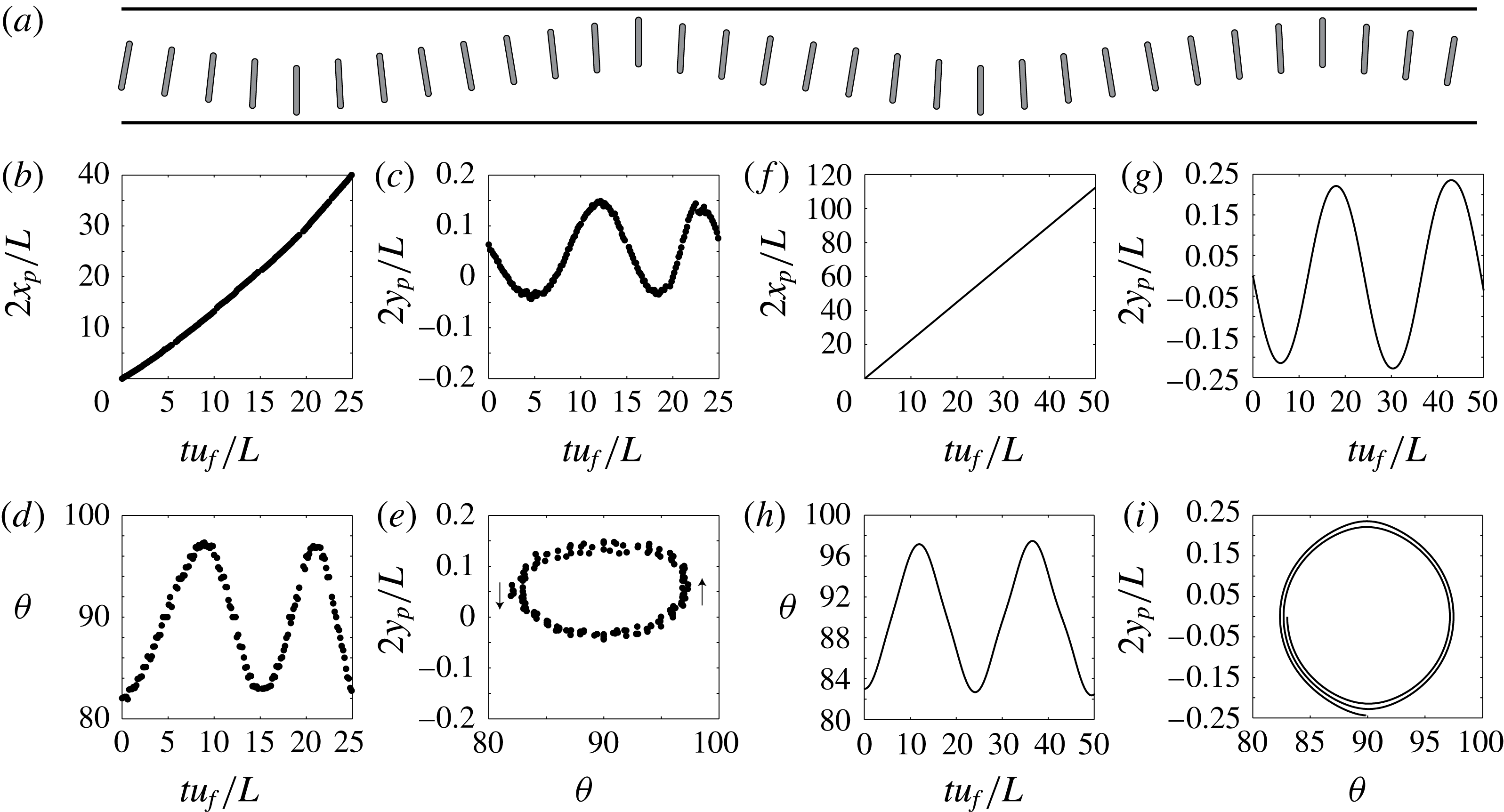
Figure 11. (a) Sketch of the oscillation mode. (b–i) Trajectory of a fibre advected by a mean flow for
 $\unicode[STIX]{x1D6FD}=0.78$
,
$\unicode[STIX]{x1D6FD}=0.78$
,
 $\unicode[STIX]{x1D709}=0.63$
and
$\unicode[STIX]{x1D709}=0.63$
and
 $\unicode[STIX]{x1D703}_{i}=82^{\circ }$
obtained experimentally (b–e) and numerically (f–i). (b,f) Axial position
$\unicode[STIX]{x1D703}_{i}=82^{\circ }$
obtained experimentally (b–e) and numerically (f–i). (b,f) Axial position
 $x_{p}(t)$
, (c,g) streamwise position
$x_{p}(t)$
, (c,g) streamwise position
 $y_{p}(t)$
, (d,h) orientation
$y_{p}(t)$
, (d,h) orientation
 $\unicode[STIX]{x1D703}(t)$
and (e,i) orbit
$\unicode[STIX]{x1D703}(t)$
and (e,i) orbit
 $y_{p}(\unicode[STIX]{x1D703})$
. All lengths are made dimensionless using
$y_{p}(\unicode[STIX]{x1D703})$
. All lengths are made dimensionless using
 $L/2$
, and time is normalized with the fibre velocity and channel length, i.e.
$L/2$
, and time is normalized with the fibre velocity and channel length, i.e.
 $L/u_{f}$
. The experimental trajectory corresponds to the experiments shown in figure 1.
$L/u_{f}$
. The experimental trajectory corresponds to the experiments shown in figure 1.
4.2.3 Trajectories near the walls
As seen previously, there is a layer near the wall which is not accessible through glancing (shaded area in figure 10
b). If the fibres are not initially placed at the centre of the channel but in this layer, that is in the vicinity of the wall, we can access different types of trajectories. To investigate the occurrence of these trajectories we position the fibre horizontally (
 $\unicode[STIX]{x1D703}_{i}=0^{\circ }$
) close to the wall
$\unicode[STIX]{x1D703}_{i}=0^{\circ }$
) close to the wall
 $y_{i}\simeq y_{w}$
and observe the resulting trajectories as a function of the distance
$y_{i}\simeq y_{w}$
and observe the resulting trajectories as a function of the distance
 $1-y_{i}$
(figure 12).
$1-y_{i}$
(figure 12).
For
 $y_{i}\leqslant y_{w}$
, the fibre rotates and drifts away at a constant angle as described in the previous sections. As we decrease the distance to the wall
$y_{i}\leqslant y_{w}$
, the fibre rotates and drifts away at a constant angle as described in the previous sections. As we decrease the distance to the wall
 $1-y_{i}$
, another situation occurs, as presented in (figure 12
a). The fibre remains near one wall, does not oscillate between the walls, but rotates around its tip in a pole-vaulting motion (Stover & Cohen Reference Stover and Cohen1990). In that case, the orbit is open (figure 12
c). We note that only a small difference in distance to the wall leads to the transition between pole-vaulting and glancing motions (figure 12
e). In fact, for large angles where fibre oscillation amplitudes are large, the fibre may alternate between those two types of motion as it moves downstream. Another situation occurs for even smaller fibre–wall distances
$1-y_{i}$
, another situation occurs, as presented in (figure 12
a). The fibre remains near one wall, does not oscillate between the walls, but rotates around its tip in a pole-vaulting motion (Stover & Cohen Reference Stover and Cohen1990). In that case, the orbit is open (figure 12
c). We note that only a small difference in distance to the wall leads to the transition between pole-vaulting and glancing motions (figure 12
e). In fact, for large angles where fibre oscillation amplitudes are large, the fibre may alternate between those two types of motion as it moves downstream. Another situation occurs for even smaller fibre–wall distances
 $1-y_{i}$
. The fibre remains in a layer near the wall, exhibiting small amplitude oscillations that we call wiggling (figure 12
b). The angle remains close to
$1-y_{i}$
. The fibre remains in a layer near the wall, exhibiting small amplitude oscillations that we call wiggling (figure 12
b). The angle remains close to
 $0^{\circ }$
(figure 12
d). The orbit is confined in a small parameter range (figure 12
e). Our numerical simulations recover these two trajectories, as shown in figure 12. Numerically, we investigate the occurrence of these trajectories in a similar fashion as in the experiments: we place the fibre, either horizontally or vertically, at different distances from the wall and record its rotation rate
$0^{\circ }$
(figure 12
d). The orbit is confined in a small parameter range (figure 12
e). Our numerical simulations recover these two trajectories, as shown in figure 12. Numerically, we investigate the occurrence of these trajectories in a similar fashion as in the experiments: we place the fibre, either horizontally or vertically, at different distances from the wall and record its rotation rate
 $\dot{\unicode[STIX]{x1D703}_{p}}$
(figure 6
b). For a fibre placed horizontally (i.e. parallel to the flow), we observe that the rotation rate becomes slightly positive very near the wall (
$\dot{\unicode[STIX]{x1D703}_{p}}$
(figure 6
b). For a fibre placed horizontally (i.e. parallel to the flow), we observe that the rotation rate becomes slightly positive very near the wall (
 $y_{p}\leqslant 0.9$
), which indicates the transition to wiggling. Similarly, for a fibre placed vertically (i.e. perpendicular to the flow), the rotation rate becomes negative when approaching the wall, indicating a transition to pole vaulting.
$y_{p}\leqslant 0.9$
), which indicates the transition to wiggling. Similarly, for a fibre placed vertically (i.e. perpendicular to the flow), the rotation rate becomes negative when approaching the wall, indicating a transition to pole vaulting.

Figure 12. Chronophotographs of a fibre flowing near the wall for
 $\unicode[STIX]{x1D6FD}=0.81$
,
$\unicode[STIX]{x1D6FD}=0.81$
,
 $\unicode[STIX]{x1D709}=0.81$
, exhibiting (a) pole vaulting and (b) wiggling, obtained both experimentally (top) and numerically (bottom). (c) Orbit for pole vaulting for
$\unicode[STIX]{x1D709}=0.81$
, exhibiting (a) pole vaulting and (b) wiggling, obtained both experimentally (top) and numerically (bottom). (c) Orbit for pole vaulting for
 $\unicode[STIX]{x1D6FD}=0.78$
,
$\unicode[STIX]{x1D6FD}=0.78$
,
 $\unicode[STIX]{x1D709}=0.93$
. (d) Orbit for wiggling for
$\unicode[STIX]{x1D709}=0.93$
. (d) Orbit for wiggling for
 $\unicode[STIX]{x1D6FD}=0.75$
,
$\unicode[STIX]{x1D6FD}=0.75$
,
 $\unicode[STIX]{x1D709}=0.17$
. (e) Trajectories near the walls for
$\unicode[STIX]{x1D709}=0.17$
. (e) Trajectories near the walls for
 $\unicode[STIX]{x1D6FD}=0.86$
,
$\unicode[STIX]{x1D6FD}=0.86$
,
 $\unicode[STIX]{x1D709}=0.16$
. Numerical simulations with the same parameters are shown in solid lines. For (e) the numerical pole-vaulting and glancing trajectories become so close that they are indistinguishable near the wall.
$\unicode[STIX]{x1D709}=0.16$
. Numerical simulations with the same parameters are shown in solid lines. For (e) the numerical pole-vaulting and glancing trajectories become so close that they are indistinguishable near the wall.
4.3 State diagram
We build a state diagram in the parameter space (
 $\unicode[STIX]{x1D703}_{p}$
,
$\unicode[STIX]{x1D703}_{p}$
,
 $y_{p}$
) to identify the various trajectories and isolate the regions in the parameter space where the different types of dynamics occur. We first present the diagram corresponding to a regime of high confinement, both transverse and lateral (
$y_{p}$
) to identify the various trajectories and isolate the regions in the parameter space where the different types of dynamics occur. We first present the diagram corresponding to a regime of high confinement, both transverse and lateral (
 $\unicode[STIX]{x1D6FD}=0.8$
and
$\unicode[STIX]{x1D6FD}=0.8$
and
 $\unicode[STIX]{x1D709}=0.8$
) (figure 13). We report a remarkable agreement between experiments and simulations, showing that our 2-D scheme captures the physics of this 3-D problem. In addition, the numerical simulations give access to all possible trajectories to obtain a complete diagram. The experimental glancing orbit shows a spiralling behaviour that is absent in the simulation, and that will be discussed further in § 5.
$\unicode[STIX]{x1D709}=0.8$
) (figure 13). We report a remarkable agreement between experiments and simulations, showing that our 2-D scheme captures the physics of this 3-D problem. In addition, the numerical simulations give access to all possible trajectories to obtain a complete diagram. The experimental glancing orbit shows a spiralling behaviour that is absent in the simulation, and that will be discussed further in § 5.

Figure 13. Experimental (
 $\unicode[STIX]{x1D6FD}\simeq 0.8$
,
$\unicode[STIX]{x1D6FD}\simeq 0.8$
,
 $\unicode[STIX]{x1D709}\simeq 0.8$
, black dots) and numerical state diagram (
$\unicode[STIX]{x1D709}\simeq 0.8$
, black dots) and numerical state diagram (
 $\unicode[STIX]{x1D6FD}=0.8$
,
$\unicode[STIX]{x1D6FD}=0.8$
,
 $\unicode[STIX]{x1D709}=0.8$
, grey lines). Experimental results retrace the numerical orbits for glancing (around
$\unicode[STIX]{x1D709}=0.8$
, grey lines). Experimental results retrace the numerical orbits for glancing (around
 $\pm 30^{\circ }$
) in light grey and pole vaulting in dark grey. The region in white corresponds to impossible configurations, i.e. the fibre tip touches the wall.
$\pm 30^{\circ }$
) in light grey and pole vaulting in dark grey. The region in white corresponds to impossible configurations, i.e. the fibre tip touches the wall.
We can observe the pole-vaulting orbits, centred on
 $\unicode[STIX]{x1D703}_{p}=90^{\circ }$
, and the glancing orbits, i.e. oscillations around the fixed point at
$\unicode[STIX]{x1D703}_{p}=90^{\circ }$
, and the glancing orbits, i.e. oscillations around the fixed point at
 $\unicode[STIX]{x1D703}_{p}=0^{\circ }$
. For these values of
$\unicode[STIX]{x1D703}_{p}=0^{\circ }$
. For these values of
 $\unicode[STIX]{x1D6FD}$
and
$\unicode[STIX]{x1D6FD}$
and
 $\unicode[STIX]{x1D709}$
, reversing oscillations are never observed, neither experimentally nor numerically.
$\unicode[STIX]{x1D709}$
, reversing oscillations are never observed, neither experimentally nor numerically.
The obtained state diagram is reminiscent of that of an undamped perfect pendulum (Strogatz Reference Strogatz1994). It is characteristic of an Hamiltonian system, with time-reversal symmetry. In the present case, this property does not result from the absence of dissipation in the system, but from the symmetries of the fibre and the reciprocal properties of the Stokes equations. The orbits can be categorized exactly like for a pendulum. The pole-vaulting orbits are free (unbounded) trajectories, while the glancing orbits are bound states and both are separated by a separatrix. The state diagram is organized around two centres, the stable
 $\unicode[STIX]{x1D703}_{p}=0^{\circ },y_{p}=0$
horizontal position and the structurally unstable hyperbolic centre corresponding to the vertically aligned fibre
$\unicode[STIX]{x1D703}_{p}=0^{\circ },y_{p}=0$
horizontal position and the structurally unstable hyperbolic centre corresponding to the vertically aligned fibre
 $\unicode[STIX]{x1D703}_{p}=90^{\circ },y_{p}=0$
.
$\unicode[STIX]{x1D703}_{p}=90^{\circ },y_{p}=0$
.
While, as stated earlier, reversing orbits could not been observed for the parameters of figure 13, they can be obtained for lower values of the lateral confinement
 $\unicode[STIX]{x1D709}$
. For
$\unicode[STIX]{x1D709}$
. For
 $\unicode[STIX]{x1D6FD}=0.8$
, reversing is only obtained for
$\unicode[STIX]{x1D6FD}=0.8$
, reversing is only obtained for
 $\unicode[STIX]{x1D709}\leqslant 0.6$
as observed in the experiments (figure 11). This regime is further explored numerically and a complete state diagram for this value is presented in figure 14. In addition to glancing, pole vaulting and wiggling, reversing can be observed in the vicinity of
$\unicode[STIX]{x1D709}\leqslant 0.6$
as observed in the experiments (figure 11). This regime is further explored numerically and a complete state diagram for this value is presented in figure 14. In addition to glancing, pole vaulting and wiggling, reversing can be observed in the vicinity of
 $\unicode[STIX]{x1D703}_{p}=90^{\circ }$
. This diagram is also characteristic of Hamiltonian dynamics, but it is more complex than that of a simple pendulum. It has stable centres at
$\unicode[STIX]{x1D703}_{p}=90^{\circ }$
. This diagram is also characteristic of Hamiltonian dynamics, but it is more complex than that of a simple pendulum. It has stable centres at
 $\unicode[STIX]{x1D703}_{p}=0^{\circ },180^{\circ },y_{p}=0$
,
$\unicode[STIX]{x1D703}_{p}=0^{\circ },180^{\circ },y_{p}=0$
,
 $\unicode[STIX]{x1D703}_{p}=\pm 90^{\circ },y_{p}=0$
and
$\unicode[STIX]{x1D703}_{p}=\pm 90^{\circ },y_{p}=0$
and
 $\unicode[STIX]{x1D703}_{p}=0^{\circ },180^{\circ },y_{p}\approx \pm 0.92$
as well as unstable hyperbolic centres at
$\unicode[STIX]{x1D703}_{p}=0^{\circ },180^{\circ },y_{p}\approx \pm 0.92$
as well as unstable hyperbolic centres at
 $\unicode[STIX]{x1D703}_{p}=\pm 90^{\circ },y_{p}\approx \pm 0.32$
and
$\unicode[STIX]{x1D703}_{p}=\pm 90^{\circ },y_{p}\approx \pm 0.32$
and
 $\unicode[STIX]{x1D703}_{p}=0^{\circ },180^{\circ },y_{p}\approx \pm 0.9$
. These fix points structure the phase space which has dynamics with three types of bound states, glancing, reversing and wiggling orbits and separatrices that connect the hyperbolic points.
$\unicode[STIX]{x1D703}_{p}=0^{\circ },180^{\circ },y_{p}\approx \pm 0.9$
. These fix points structure the phase space which has dynamics with three types of bound states, glancing, reversing and wiggling orbits and separatrices that connect the hyperbolic points.

Figure 14. Numerical state diagram for
 $\unicode[STIX]{x1D6FD}=0.8$
,
$\unicode[STIX]{x1D6FD}=0.8$
,
 $\unicode[STIX]{x1D709}=0.6$
. displaying all four orbit types: glancing, reversing, pole vaulting and wiggling together with their associated fix points. Separatrices exist in between the coloured regions, where the numerical scheme was unable to resolve trajectories the colour is left grey. The region in white corresponds to impossible configurations, i.e. the fibre tip touches the wall.
$\unicode[STIX]{x1D709}=0.6$
. displaying all four orbit types: glancing, reversing, pole vaulting and wiggling together with their associated fix points. Separatrices exist in between the coloured regions, where the numerical scheme was unable to resolve trajectories the colour is left grey. The region in white corresponds to impossible configurations, i.e. the fibre tip touches the wall.
From a theoretical point of view, the motion of a fibre is completely described by the coordinates
 $y_{p}$
and
$y_{p}$
and
 $\unicode[STIX]{x1D703}_{p}$
for a given configuration in a rectangular channel. Therefore, in theory, the trajectories in the state diagram are, apart from singular points, free of intersections and consequently closed loops. However, in both experimental and numerical diagrams, the orbits are close to each other, especially near the walls (along the pole-vaulting separatrix) and at the glancing–reversing limit. As a result, the fibre easily jumps from one orbit to another, as we will discuss in the next paragraph.
$\unicode[STIX]{x1D703}_{p}$
for a given configuration in a rectangular channel. Therefore, in theory, the trajectories in the state diagram are, apart from singular points, free of intersections and consequently closed loops. However, in both experimental and numerical diagrams, the orbits are close to each other, especially near the walls (along the pole-vaulting separatrix) and at the glancing–reversing limit. As a result, the fibre easily jumps from one orbit to another, as we will discuss in the next paragraph.
5 Discussion
5.1 Glancing
We first investigate the glancing trajectories. The trajectory of a fibre is a combination of drift, due to drag anisotropy, and rotation due to the presence of the lateral walls. We can compute numerically both the vertical drift velocity
 $\dot{y_{p}}$
, and the rotation velocity
$\dot{y_{p}}$
, and the rotation velocity
 $\dot{\unicode[STIX]{x1D703}_{p}}$
. We compare the evolution of these velocities as the fibre oscillates between the walls for two different initial angles (figure 15). As the fibre travels from the bottom wall to the centre of the channel, the drift velocity increases (with
$\dot{\unicode[STIX]{x1D703}_{p}}$
. We compare the evolution of these velocities as the fibre oscillates between the walls for two different initial angles (figure 15). As the fibre travels from the bottom wall to the centre of the channel, the drift velocity increases (with
 $\dot{y_{p}}>0$
) while the fibre rotates away for a horizontal orientation (
$\dot{y_{p}}>0$
) while the fibre rotates away for a horizontal orientation (
 $\dot{\unicode[STIX]{x1D703}_{p}}<0^{\circ }$
). Near the centre of the channel, the rotation velocity
$\dot{\unicode[STIX]{x1D703}_{p}}<0^{\circ }$
). Near the centre of the channel, the rotation velocity
 $\dot{\unicode[STIX]{x1D703}_{p}}=0^{\circ }$
and the curve present an inflection point; the orientation of the fibre is thus constant, which leads to a constant drift velocity as seen in figure 15(a). As the fibre travels away from the centre and approaches the wall, the drift velocity rapidly decreases to reach zero when the fibre is horizontal, and the rotation velocity increases as the fibre reorients (
$\dot{\unicode[STIX]{x1D703}_{p}}=0^{\circ }$
and the curve present an inflection point; the orientation of the fibre is thus constant, which leads to a constant drift velocity as seen in figure 15(a). As the fibre travels away from the centre and approaches the wall, the drift velocity rapidly decreases to reach zero when the fibre is horizontal, and the rotation velocity increases as the fibre reorients (
 $\dot{\unicode[STIX]{x1D703}_{p}}>0^{\circ }$
). The top to bottom trajectory is symmetrical (with
$\dot{\unicode[STIX]{x1D703}_{p}}>0^{\circ }$
). The top to bottom trajectory is symmetrical (with
 $\dot{y_{p}}<0$
).
$\dot{y_{p}}<0$
).
We note that the drift velocity strongly depends on the fibre angle (
 $\dot{y_{p}}(\unicode[STIX]{x1D703}=20^{\circ })\simeq 2\dot{y_{p}}(\unicode[STIX]{x1D703}=10^{\circ })$
). Indeed, the drift velocity, given in (4.2), is proportional to
$\dot{y_{p}}(\unicode[STIX]{x1D703}=20^{\circ })\simeq 2\dot{y_{p}}(\unicode[STIX]{x1D703}=10^{\circ })$
). Indeed, the drift velocity, given in (4.2), is proportional to
 $\cos \unicode[STIX]{x1D703}\sin \unicode[STIX]{x1D703}$
. The drift velocity thus increases almost linearly with the orientation angle up to
$\cos \unicode[STIX]{x1D703}\sin \unicode[STIX]{x1D703}$
. The drift velocity thus increases almost linearly with the orientation angle up to
 $\unicode[STIX]{x1D703}=45^{\circ }$
. On the contrary, the rotation velocity is nearly independent of the fibre angle.
$\unicode[STIX]{x1D703}=45^{\circ }$
. On the contrary, the rotation velocity is nearly independent of the fibre angle.
These results qualitatively explain the observations made on the fibre trajectories. The fibre drifts and rotates simultaneously. Since the rotation velocity is nearly constant, the maximum displacement
 $|y_{p}|$
of the motion depends on the drift velocity: the faster the drift velocity, the further the fibre can travel in the channel. Indeed, as we increase the initial angle, the rotation velocity is unaffected while the drift velocity strongly increases, leading to larger amplitude oscillations (i.e. the fibre travels a longer distance before it is rotated, hence glances closer to the wall). On the contrary, small angles lead to slow drift velocities and to small amplitude oscillations, so that a fibre whose orientation is close to zero remains in the centre of the channel.
$|y_{p}|$
of the motion depends on the drift velocity: the faster the drift velocity, the further the fibre can travel in the channel. Indeed, as we increase the initial angle, the rotation velocity is unaffected while the drift velocity strongly increases, leading to larger amplitude oscillations (i.e. the fibre travels a longer distance before it is rotated, hence glances closer to the wall). On the contrary, small angles lead to slow drift velocities and to small amplitude oscillations, so that a fibre whose orientation is close to zero remains in the centre of the channel.
Furthermore, as we increase the confinement, we can tune the difference between
 $u_{\Vert }$
and
$u_{\Vert }$
and
 $u_{\bot }$
, and thus increase the drift velocity (
$u_{\bot }$
, and thus increase the drift velocity (
 $\dot{y_{p}}\propto (u_{\Vert }-u_{\bot })$
) and the oscillation amplitude, as observed experimentally and numerically.
$\dot{y_{p}}\propto (u_{\Vert }-u_{\bot })$
) and the oscillation amplitude, as observed experimentally and numerically.

Figure 15. Evolution of the drift velocity
 $v_{p}=\text{d}y_{p}/\text{d}t$
(a) and the rotation velocity
$v_{p}=\text{d}y_{p}/\text{d}t$
(a) and the rotation velocity
 $\dot{\unicode[STIX]{x1D703}}=\text{d}\unicode[STIX]{x1D703}/\text{d}t$
(b) as a function of the fibre position
$\dot{\unicode[STIX]{x1D703}}=\text{d}\unicode[STIX]{x1D703}/\text{d}t$
(b) as a function of the fibre position
 $y_{p}$
as the fibre oscillates between the walls. Computed for
$y_{p}$
as the fibre oscillates between the walls. Computed for
 $\unicode[STIX]{x1D6FD}=0.8$
and
$\unicode[STIX]{x1D6FD}=0.8$
and
 $\unicode[STIX]{x1D709}=0.8$
and for two initial angles
$\unicode[STIX]{x1D709}=0.8$
and for two initial angles
 $\unicode[STIX]{x1D703}_{i}=10^{\circ }$
(dashed line, grey) and
$\unicode[STIX]{x1D703}_{i}=10^{\circ }$
(dashed line, grey) and
 $\unicode[STIX]{x1D703}_{i}=20^{\circ }$
(full line, black).
$\unicode[STIX]{x1D703}_{i}=20^{\circ }$
(full line, black).
5.2 Transition between glancing and reversing
During an oscillation in the reversing regime, the evolution of the drift velocity is analogous to glancing. Similarly, the drift velocity decreases when approaching
 $\unicode[STIX]{x1D703}_{p}=90^{\circ }$
so that the amplitude of the oscillations decreases as the fibre angle gets closer to
$\unicode[STIX]{x1D703}_{p}=90^{\circ }$
so that the amplitude of the oscillations decreases as the fibre angle gets closer to
 $\unicode[STIX]{x1D703}_{p}=90^{\circ }$
(as can be seen from the state diagram figure 14). However, the sign of the rotation speed is inverted (i.e. the angle decreases as the fibre leaves the wall and increases as the fibre approaches a wall, in an opposite fashion compared to the glancing regime). The transition between glancing and reversing can be obtained by looking at the sign of the rotation speed. We obtain the critical angle
$\unicode[STIX]{x1D703}_{p}=90^{\circ }$
(as can be seen from the state diagram figure 14). However, the sign of the rotation speed is inverted (i.e. the angle decreases as the fibre leaves the wall and increases as the fibre approaches a wall, in an opposite fashion compared to the glancing regime). The transition between glancing and reversing can be obtained by looking at the sign of the rotation speed. We obtain the critical angle
 $\unicode[STIX]{x1D703}^{\star }$
for which the transition occurs for different confinements. For
$\unicode[STIX]{x1D703}^{\star }$
for which the transition occurs for different confinements. For
 $\unicode[STIX]{x1D709}\sim 0.8$
, the value of
$\unicode[STIX]{x1D709}\sim 0.8$
, the value of
 $\unicode[STIX]{x1D703}^{\star }$
remains close to
$\unicode[STIX]{x1D703}^{\star }$
remains close to
 $90^{\circ }$
, and slightly decreases for increasing confinement
$90^{\circ }$
, and slightly decreases for increasing confinement
 $\unicode[STIX]{x1D6FD}$
. This explains why reversing is difficult to observe at high lateral confinement, where the region of reversing in the parameter space is narrow around
$\unicode[STIX]{x1D6FD}$
. This explains why reversing is difficult to observe at high lateral confinement, where the region of reversing in the parameter space is narrow around
 $90^{\circ }$
. The reversing region expands when decreasing
$90^{\circ }$
. The reversing region expands when decreasing
 $\unicode[STIX]{x1D709}$
. Experimentally, we indeed observe systematically reversing in the wide channels (
$\unicode[STIX]{x1D709}$
. Experimentally, we indeed observe systematically reversing in the wide channels (
 $\unicode[STIX]{x1D709}=O(10^{-2})$
). However, in such wide channels it is not possible to follow an entire oscillation as the fibre travels through a long distance between the walls. We thus limit ourselves to the trajectories near one wall (figure 16). Numerically, we observe that the reversing region expands when decreasing
$\unicode[STIX]{x1D709}=O(10^{-2})$
). However, in such wide channels it is not possible to follow an entire oscillation as the fibre travels through a long distance between the walls. We thus limit ourselves to the trajectories near one wall (figure 16). Numerically, we observe that the reversing region expands when decreasing
 $\unicode[STIX]{x1D709}$
, i.e.
$\unicode[STIX]{x1D709}$
, i.e.
 $\unicode[STIX]{x1D703}^{\star }$
decreases to approach zero. While in highly confined channels (
$\unicode[STIX]{x1D703}^{\star }$
decreases to approach zero. While in highly confined channels (
 $\unicode[STIX]{x1D709}\sim 1$
), reversing is confined in a narrow region around
$\unicode[STIX]{x1D709}\sim 1$
), reversing is confined in a narrow region around
 $90^{\circ }$
, for low confinement this region can reach larger regions (as observed in figures 14 and 16). We also note that the limit orbit between reversing and glancing is peculiar (see the line separating the yellow and blue regions in figure 14); indeed, the angle first increases then decreases as the fibre approaches the wall. This can also be observed experimentally (figure 16). The corresponding orbits are given for
$90^{\circ }$
, for low confinement this region can reach larger regions (as observed in figures 14 and 16). We also note that the limit orbit between reversing and glancing is peculiar (see the line separating the yellow and blue regions in figure 14); indeed, the angle first increases then decreases as the fibre approaches the wall. This can also be observed experimentally (figure 16). The corresponding orbits are given for
 $\unicode[STIX]{x1D709}=0.14$
and initial angles around
$\unicode[STIX]{x1D709}=0.14$
and initial angles around
 $25^{\circ }$
, at the limit of glancing, reversing and pole vaulting. We note the reversing (dark grey) and pole-vaulting (light grey) trajectories. For the glancing trajectory (black), the fibre drifts near the centre of the channel, its angle increases as in the reversing trajectory, however the angle then decreases to reach zero in a glancing motion. Similarly, upon leaving the wall, the angle first increases then decreases.
$25^{\circ }$
, at the limit of glancing, reversing and pole vaulting. We note the reversing (dark grey) and pole-vaulting (light grey) trajectories. For the glancing trajectory (black), the fibre drifts near the centre of the channel, its angle increases as in the reversing trajectory, however the angle then decreases to reach zero in a glancing motion. Similarly, upon leaving the wall, the angle first increases then decreases.

Figure 16. Trajectory obtained experimentally for
 $\unicode[STIX]{x1D6FD}=0.76$
,
$\unicode[STIX]{x1D6FD}=0.76$
,
 $\unicode[STIX]{x1D709}=0.14$
. (a) Orbits. (b) Chronophotography of the limit trajectory between glancing, reversing and pole vaulting. The channel being wide, we only display a region near the bottom wall, i.e.
$\unicode[STIX]{x1D709}=0.14$
. (a) Orbits. (b) Chronophotography of the limit trajectory between glancing, reversing and pole vaulting. The channel being wide, we only display a region near the bottom wall, i.e.
 $-0.5>y_{p}>-1$
.
$-0.5>y_{p}>-1$
.
5.3 Transition between wiggling, pole vaulting and glancing
While the flow within the rectangular channel is a plug flow throughout most of the width of the channel, there is a small layer near the walls, of size
 ${\sim}\,H$
, where there is shear due to the no-slip condition at the wall. For the data presented in figure 10(b), the boundary layer thickness corresponds to
${\sim}\,H$
, where there is shear due to the no-slip condition at the wall. For the data presented in figure 10(b), the boundary layer thickness corresponds to
 $|1-y_{w}|\simeq 0.1$
, i.e. during glancing the fibre always remains outside the boundary layer. When placed within the boundary layer, the fibre exhibits different trajectories, i.e. either a pole-vaulting or a wiggling motion.
$|1-y_{w}|\simeq 0.1$
, i.e. during glancing the fibre always remains outside the boundary layer. When placed within the boundary layer, the fibre exhibits different trajectories, i.e. either a pole-vaulting or a wiggling motion.
We can discriminate between the different trajectories using the boundary layer thickness. We rescale the data corresponding to the different trajectories near the walls (figure 12
e) with the boundary layer thickness
 $H$
, as shown in figure 17. We indeed observe that wiggling exists for
$H$
, as shown in figure 17. We indeed observe that wiggling exists for
 $y<H$
, pole vaulting for
$y<H$
, pole vaulting for
 $y\sim H$
and glancing for
$y\sim H$
and glancing for
 $y>H$
. As the fibre is entirely within the boundary layer (
$y>H$
. As the fibre is entirely within the boundary layer (
 $y<H$
), it oscillates without leaving the wall in a wiggling motion. If the fibre tip is within the boundary layer
$y<H$
), it oscillates without leaving the wall in a wiggling motion. If the fibre tip is within the boundary layer
 $y\sim H$
, the fibre may be rotated around its tip, thus exhibiting a pole-vaulting motion. For larger distances, the fibre is not affected by the shear and simply rotates away from the wall in a glancing motion.
$y\sim H$
, the fibre may be rotated around its tip, thus exhibiting a pole-vaulting motion. For larger distances, the fibre is not affected by the shear and simply rotates away from the wall in a glancing motion.

Figure 17. Trajectories near the wall (same data as figure 12
e) rescaled with channel height
 $H$
. The inset is a zoom of the data around
$H$
. The inset is a zoom of the data around
 $y/H=1$
.
$y/H=1$
.
5.4 Transition between reversing and pole vaulting
In a sufficiently wide channel, i.e. with
 $\unicode[STIX]{x1D709}$
lower than
$\unicode[STIX]{x1D709}$
lower than
 $0.8$
in the case
$0.8$
in the case
 $\unicode[STIX]{x1D6FD}=0.8$
and
$\unicode[STIX]{x1D6FD}=0.8$
and
 $\ell /h=8$
, a fibre can show reversing or pole vaulting when oriented perpendicular to the flow. For the description of reversing the presence of a potential Hele-Shaw flow (corresponding to a plug flow) is sufficient. A reversing motion has been indeed justified by image potentials (Uspal et al.
Reference Uspal, Burak Eral and Doyle2013; Shen et al.
Reference Shen, Leman, Reyssat and Tabeling2014). As the fibre enters the shear boundary layer near the lateral walls, potential flow is no longer valid and one observes a competition between a tip acceleration due to the leaking flow and tip deceleration due to wall friction. In figure 18(a) one sees a fibre performing a reversing motion, where the liquid flows through the gap between fibre tip and lateral wall. A negative vorticity is observed at the fibre tip. In comparison, if the fibre is too close to the wall no fluid leakage is observed between the fibre tip and the wall. A positive vorticity close to the fibre tip leads to a pole-vaulting motion (figure 18
b).
$\ell /h=8$
, a fibre can show reversing or pole vaulting when oriented perpendicular to the flow. For the description of reversing the presence of a potential Hele-Shaw flow (corresponding to a plug flow) is sufficient. A reversing motion has been indeed justified by image potentials (Uspal et al.
Reference Uspal, Burak Eral and Doyle2013; Shen et al.
Reference Shen, Leman, Reyssat and Tabeling2014). As the fibre enters the shear boundary layer near the lateral walls, potential flow is no longer valid and one observes a competition between a tip acceleration due to the leaking flow and tip deceleration due to wall friction. In figure 18(a) one sees a fibre performing a reversing motion, where the liquid flows through the gap between fibre tip and lateral wall. A negative vorticity is observed at the fibre tip. In comparison, if the fibre is too close to the wall no fluid leakage is observed between the fibre tip and the wall. A positive vorticity close to the fibre tip leads to a pole-vaulting motion (figure 18
b).

Figure 18. Three-dimensional simulation of a moving fibre with
 $\unicode[STIX]{x1D6FD}=0.8$
in a wide channel
$\unicode[STIX]{x1D6FD}=0.8$
in a wide channel
 $\unicode[STIX]{x1D709}=0.5$
. Shown are the data from the centre plane in
$\unicode[STIX]{x1D709}=0.5$
. Shown are the data from the centre plane in
 $z$
. Streamlines are drawn with respect to the fibres mean velocity for (a) reversing fibre and (b) pole-vaulting fibre.
$z$
. Streamlines are drawn with respect to the fibres mean velocity for (a) reversing fibre and (b) pole-vaulting fibre.
5.5 Perturbations and damped oscillations
The system is sensitive to perturbations. Any perturbation leads to a small change in orientation, thus a change in trajectory. In particular, we often observe in experiments that the fibre leaves the wall with an angle slightly smaller than the initial approaching angle. The amplitude of oscillations may thus decrease as the fibre moves along the channel. This effect may be important, leading to damped oscillations as presented in figure 19. The amplitude of the oscillations decreases and the fibre moves towards the centre of the channel, until reaching the equilibrium position, i.e. the fix point (
 $\unicode[STIX]{x1D703}_{p}=0^{\circ }$
,
$\unicode[STIX]{x1D703}_{p}=0^{\circ }$
,
 $y_{p}=0$
), staying parallel to the flow in the centre of the channel
$y_{p}=0$
), staying parallel to the flow in the centre of the channel
 $y_{p}=0$
. Uspal et al. (Reference Uspal, Burak Eral and Doyle2013) showed that a fore–aft asymmetry also leads to the reorientation of the particle towards
$y_{p}=0$
. Uspal et al. (Reference Uspal, Burak Eral and Doyle2013) showed that a fore–aft asymmetry also leads to the reorientation of the particle towards
 $\unicode[STIX]{x1D703}_{p}=0^{\circ }$
. The analogy with the pendulum’s trajectories evoked earlier (§ 4.3) can be pushed further. The addition of a slight imperfection, here taking the form of a small experimental spatial asymmetry or an experimental or numerical time-symmetry breaking, acts in a similar way as the addition of a small damping in the pendulum (Strogatz Reference Strogatz1994). While the stable orbits disappear, the previously neutrally stable centres become focal points attracting the dynamics through spiralling trajectories. This behaviour results from the structural instability of the hyperbolic fix points.
$\unicode[STIX]{x1D703}_{p}=0^{\circ }$
. The analogy with the pendulum’s trajectories evoked earlier (§ 4.3) can be pushed further. The addition of a slight imperfection, here taking the form of a small experimental spatial asymmetry or an experimental or numerical time-symmetry breaking, acts in a similar way as the addition of a small damping in the pendulum (Strogatz Reference Strogatz1994). While the stable orbits disappear, the previously neutrally stable centres become focal points attracting the dynamics through spiralling trajectories. This behaviour results from the structural instability of the hyperbolic fix points.

Figure 19. Damped oscillations obtained experimentally for
 $\unicode[STIX]{x1D6FD}=0.8$
,
$\unicode[STIX]{x1D6FD}=0.8$
,
 $\unicode[STIX]{x1D709}=0.8$
. (a) Position
$\unicode[STIX]{x1D709}=0.8$
. (a) Position
 $y$
and angle
$y$
and angle
 $\unicode[STIX]{x1D703}$
as a function of time. (b) Spiralling orbit.
$\unicode[STIX]{x1D703}$
as a function of time. (b) Spiralling orbit.
6 Conclusion
We have investigated experimentally and numerically the motion of rigid fibres confined in a Hele-Shaw cell and transported by a pressure-driven flow. Due to the transverse and lateral confinements, complex fibre oscillations between the channel walls are observed in experiments, as well as pole vaulting and ‘wiggling’ when the fibre is placed near the walls. We have shown that the trajectories can be controlled by adjusting the geometry of the fibre and the channel. We have in particular shown the effect of the transverse confinement (height of the channel), which controls the magnitude of the drag anisotropy, thus the drift angles and as a consequence the amplitude of the oscillations.
We have developed a model using the 2-D Brinkman equations that correctly describes the dynamics. By numerically solving the model equations, we can quantitatively reproduce and predict the experimental trajectories, as well as qualitatively explain the different motions and transitions. Due to the ideal setting of a numerical simulation with perfectly smooth walls and rigid fibres, clear distinctions can be made between stable and unstable flow configurations in the absence of fabrication defaults.
The glancing and reversing motion of the fibre are controlled by the pressure field that develops around the fibre. As a consequence, these can be, at least qualitatively (Uspal et al. Reference Uspal, Burak Eral and Doyle2013), described by the Darcy equation. Pole-vaulting and wiggling motions are driven by shear flow close to the walls and can therefore not be described by the Darcy equation since there is no in-plane shear contribution, requiring therefore a more elaborate approach. Interestingly, a qualitative analysis of sedimenting flows can rely solely on the Darcy equation since the pole-vaulting motion can be thought of as being part of the reversing motion and the wiggling motion being part of the glancing motion. Only in pressure-driven flows, when the drift direction is about perpendicular to the fibre orientation, pole vaulting and wiggling exist as singular limits in a boundary layer close to the walls.
From looking at the state diagram (figure 14) one sees that the fibre trajectories come very close in certain regions, which gives rise to random changes in orbits due to small perturbations, which we observed experimentally as well as numerically. The limited numerical predictability thus reflects a physically unpredictable state.
An asymmetrically designed particle has been observed to create a driving force that keeps the perturbed particle in a well-defined orbit (Uspal et al. Reference Uspal, Burak Eral and Doyle2013), where regions of close contact of orbits from different oscillatory regimes are avoided. Within the framework of our numerical method it is possible to address the behaviour of tailored asymmetric particles, as well as multiple particle interactions. In addition, we correctly account for the effect of the confinement, which can be used to tune the strength of the drag anisotropy, thus the trajectories of the particles. We believe that this extension will be useful for the investigation of design principles for the transport of rigid objects in microfluidic devices.
Our efforts in developing and implementing the routines presented in this work are made available for the community. We share the source codes and documentation of the simulation tool (ulambator.sourceforge.net) and provide online tutorials and examples (lfmi.epfl.ch/ulambator).
Acknowledgements
The authors acknowledge the help of Caroline Frot with microfabrication, and useful discussions with Howard A. Stone. The European Research Council is acknowledged for funding the work through a starting grant (ERC SimCoMiCs 280117) and a consolidator grant (ERC PaDyFlow 682367). Agence Nationale de la Recherche (ANR-DefHy) is acknowledged for partial funding of this work and travel support.
Appendix. Three-dimensional Stokes solution with the finite element method
The FEM simulation of the 3-D Stokes equation is done with FreeFEM
 $++$
(Hecht Reference Hecht2012), where the mesh is generated in a layered structure. Owing to the symmetry in the
$++$
(Hecht Reference Hecht2012), where the mesh is generated in a layered structure. Owing to the symmetry in the
 $z$
-direction only half of the domain is solved. Due to the sparse matrices, the force free condition on the fibre cannot be imposed directly. Instead, four independent problems are solved in series, with four different boundary conditions: outer flow, fibre moving at
$z$
-direction only half of the domain is solved. Due to the sparse matrices, the force free condition on the fibre cannot be imposed directly. Instead, four independent problems are solved in series, with four different boundary conditions: outer flow, fibre moving at
 $U_{p}=1$
, fibre moving at
$U_{p}=1$
, fibre moving at
 $V_{p}=1$
and fibre rotating at
$V_{p}=1$
and fibre rotating at
 $\dot{\unicode[STIX]{x1D703}}_{p}=1$
. The torque and the
$\dot{\unicode[STIX]{x1D703}}_{p}=1$
. The torque and the
 $x$
- and
$x$
- and
 $y$
- forces on the fibre are saved, and the fibre displacement is obtained from a force balance once the four calculations are completed. We use
$y$
- forces on the fibre are saved, and the fibre displacement is obtained from a force balance once the four calculations are completed. We use
 $P_{1}^{b}/P_{1}$
elements, well suited for geometries with sharp edges, where the additional degree of freedom for the velocity description (the so-called bubble) avoids spurious pressure modes. The mesh size is approximately
$P_{1}^{b}/P_{1}$
elements, well suited for geometries with sharp edges, where the additional degree of freedom for the velocity description (the so-called bubble) avoids spurious pressure modes. The mesh size is approximately
 $1.3$
million nodes, which results in approximately
$1.3$
million nodes, which results in approximately
 $5$
millions unknowns. The convergence is given for one example in the inset in figure 6.
$5$
millions unknowns. The convergence is given for one example in the inset in figure 6.


