


1. Introduction
Vortical flows are ubiquitous in nature, often occurring in the form of large-scale structures like tornadoes, cyclones, vortex streets on the leeward side of islands and mountains; vortices are observed in several industrial shear flows too. Questions regarding the conditions under which a given vortex becomes unstable have therefore received considerable attention. In this paper, we derive an analytical criterion for centrifugal instability in an axisymmetric vortex with axial flow and background rotation, and then heuristically extend the criterion to non-axisymmetric vortices.
Early studies on the prediction of instability in an inviscid, axisymmetric vortex (with no axial flow and background rotation) subject to axisymmetric perturbations were carried out by Rayleigh (Reference Rayleigh1917), who derived a necessary and sufficient condition for centrifugal instability based on physical arguments. Billant & Gallaire (Reference Billant and Gallaire2005) have extended Rayleigh’s criterion to non-axisymmetric disturbances of any azimuthal wavenumber using large-axial-wavenumber asymptotics. For the more general scenario of a two-component, two-dimensional (2C2D), inviscid base flow, i.e. a base flow described by a velocity field (
 $u(x,y),v(x,y)$
) in the Cartesian
$u(x,y),v(x,y)$
) in the Cartesian
 $(x,y)$
-plane, with no background rotation, Bayly (Reference Bayly1988) concluded that (i) the streamlines being convex closed curves in some region of the flow and (ii) the magnitude of the circulation decreasing outward are sufficient conditions for centrifugal instability.
$(x,y)$
-plane, with no background rotation, Bayly (Reference Bayly1988) concluded that (i) the streamlines being convex closed curves in some region of the flow and (ii) the magnitude of the circulation decreasing outward are sufficient conditions for centrifugal instability.
Motivated by the velocity profiles in a trailing line vortex far downstream of a wing tip and in the region upstream of a vortex breakdown in experiments, Leibovich & Stewartson (Reference Leibovich and Stewartson1983) studied axisymmetric vortices with an axial flow (and no background rotation) to derive a centrifugal instability criterion using an asymptotic analysis for large-azimuthal-wavenumber perturbations. Billant & Gallaire (Reference Billant and Gallaire2013) have further extended the study of Leibovich & Stewartson (Reference Leibovich and Stewartson1983) to the case of large total wavenumber. Gallaire & Chomaz (Reference Gallaire and Chomaz2003a ), using asymptotic expansions, have shown that centrifugal instability is active for all azimuthal wavenumbers in the axisymmetric screened Rankine vortex with a plug axial flow. Centrifugal instability has also been shown to be an important mechanism in the selection of the double-helix structure in realistic axisymmetric swirling jet flows (Gallaire & Chomaz Reference Gallaire and Chomaz2003b ). Recently, Mathur et al. (Reference Mathur, Ortiz, Dubos and Chomaz2014) investigated the effects of an axial flow on the centrifugal instability of Stuart vortices, a class of non-axisymmetric vortices that model mixing layer vortices. Solving the local stability equations numerically and also heuristically, deriving a criterion for centrifugal instability in non-axisymmetric vortices with no background rotation, Mathur et al. (Reference Mathur, Ortiz, Dubos and Chomaz2014) estimated a threshold value of the axial velocity gradient above which streamlines of the Stuart vortices become centrifugally unstable.
To model geophysical flows, Kloosterziel & van Heijst (Reference Kloosterziel and van Heijst1991) performed laboratory experiments and inferred, as a rule of thumb, that in a rotating fluid, only very weak anticyclonic, barotropic vortices are centrifugally stable, and only very strong cyclonic, barotropic vortices are centrifugally unstable. Three-dimensional direct numerical simulations (Potylitsin & Peltier Reference Potylitsin and Peltier2003) have further shown the centrifugal destabilization of columnar anticyclonic vortices subjected to weak rotation. An analytical centrifugal instability criterion for axisymmetric vortices (with no axial flow) with background rotation was derived by Mutabazi, Normand & Wesfreid (Reference Mutabazi, Normand and Wesfreid1992). Three-dimensional linear stability analysis, using both the normal mode and the local stability approaches, of the non-axisymmetric Stuart vortices with background rotation have shown centrifugal instability to be a potential reason for instability in anticyclonic vortices (Leblanc & Cambon Reference Leblanc and Cambon1998; Potylitsin & Peltier Reference Potylitsin and Peltier1999; Godeferd, Cambon & Leblanc Reference Godeferd, Cambon and Leblanc2001). In the Taylor–Green vortices of a specific aspect ratio with background rotation and no axial flow, Sipp, Lauga & Jacquin (Reference Sipp, Lauga and Jacquin1999) have shown the anticyclones to be centrifugally unstable if the Rossby number is larger than a threshold value. For the general case of any 2C2D flow in the presence of background rotation, Sipp & Jacquin (Reference Sipp and Jacquin2000) used the local stability approach to derive a sufficient condition for centrifugal instability, which accurately captures most of the centrifugally unstable streamlines only in highly concentrated Stuart vortices.
To the best of our knowledge, no existing centrifugal instability criterion accounts for the combined effects of axial flow and background rotation. The current paper addresses this gap, and is organized as follows. Adopting the local stability approach (Lifschitz & Hameiri Reference Lifschitz and Hameiri1991), we derive an analytical centrifugal instability criterion for axisymmetric vortices, and then extend it to non-axisymmetric vortices in § 2. The validity of our criterion in describing centrifugal instability in Stuart vortices and Taylor–Green vortices is investigated in § 3, followed by our discussion and conclusions in § 4.
2. Theory
We start by analytically solving the local stability equations for an inviscid, incompressible, steady, axisymmetric vortex (in the
 $xy$
-plane) with an axial velocity,
$xy$
-plane) with an axial velocity,
 $w\boldsymbol{e}_{\boldsymbol{z}}$
, and a background rotation,
$w\boldsymbol{e}_{\boldsymbol{z}}$
, and a background rotation,
 ${\it\bf\Omega}_{\!\boldsymbol{B}}={\it\Omega}_{z}\boldsymbol{e}_{\boldsymbol{z}}$
, where
${\it\bf\Omega}_{\!\boldsymbol{B}}={\it\Omega}_{z}\boldsymbol{e}_{\boldsymbol{z}}$
, where
 $\boldsymbol{e}_{\boldsymbol{z}}$
is the unit vector along the
$\boldsymbol{e}_{\boldsymbol{z}}$
is the unit vector along the
 $z$
direction. The base flow is described by a streamfunction
$z$
direction. The base flow is described by a streamfunction
 ${\it\psi}(r)$
, with the velocity components along
${\it\psi}(r)$
, with the velocity components along
 $\boldsymbol{e}_{\boldsymbol{r}}$
,
$\boldsymbol{e}_{\boldsymbol{r}}$
,
 $\boldsymbol{e}_{{\it\theta}}$
and
$\boldsymbol{e}_{{\it\theta}}$
and
 $\boldsymbol{e}_{\boldsymbol{z}}$
in cylindrical polar coordinates given by
$\boldsymbol{e}_{\boldsymbol{z}}$
in cylindrical polar coordinates given by
 $u_{r}=-(1/r)(\partial {\it\psi}/\partial {\it\theta})=0$
,
$u_{r}=-(1/r)(\partial {\it\psi}/\partial {\it\theta})=0$
,
 $u_{{\it\theta}}={\it\psi}^{\prime }$
and
$u_{{\it\theta}}={\it\psi}^{\prime }$
and
 $u_{z}=w(r)$
, respectively; the prime denotes the derivative with respect to
$u_{z}=w(r)$
, respectively; the prime denotes the derivative with respect to
 $r=\sqrt{x^{2}+y^{2}}$
. The velocity field of the base flow is thus
$r=\sqrt{x^{2}+y^{2}}$
. The velocity field of the base flow is thus
 $\boldsymbol{U}_{\!\boldsymbol{B}}={\it\psi}^{\prime }(r)\boldsymbol{e}_{{\it\theta}}+w(r)\boldsymbol{e}_{\boldsymbol{z}}$
.
$\boldsymbol{U}_{\!\boldsymbol{B}}={\it\psi}^{\prime }(r)\boldsymbol{e}_{{\it\theta}}+w(r)\boldsymbol{e}_{\boldsymbol{z}}$
.
2.1. Local stability equations
Linearized equations governing the velocity and pressure perturbations in an inviscid, incompressible flow are
 $$\begin{eqnarray}\displaystyle & \boldsymbol{{\rm\nabla}}\boldsymbol{\cdot }\boldsymbol{u}=0, & \displaystyle\end{eqnarray}$$
 $$\begin{eqnarray}\displaystyle & \displaystyle \frac{\partial \boldsymbol{u}}{\partial t}+(\boldsymbol{U}_{\!\boldsymbol{B}}\boldsymbol{\cdot }\boldsymbol{{\rm\nabla}})\boldsymbol{u}+(\boldsymbol{u}\boldsymbol{\cdot }\boldsymbol{{\rm\nabla}})\boldsymbol{U}_{\!\boldsymbol{B}}+2({\it\bf\Omega}_{\!\boldsymbol{B}}\times \boldsymbol{u})+\boldsymbol{{\rm\nabla}}P=0, & \displaystyle\end{eqnarray}$$
 $\boldsymbol{u}$
and
$\boldsymbol{u}$
and
 $p$
are the perturbations in velocity and pressure, respectively,
$p$
are the perturbations in velocity and pressure, respectively,
 $P=p/{\it\rho}_{0}$
and
$P=p/{\it\rho}_{0}$
and
 ${\it\rho}_{0}$
is the constant density. We consider short-wavelength perturbations (Godeferd et al.
Reference Godeferd, Cambon and Leblanc2001) in the limit of the WKBJ approximation:
${\it\rho}_{0}$
is the constant density. We consider short-wavelength perturbations (Godeferd et al.
Reference Godeferd, Cambon and Leblanc2001) in the limit of the WKBJ approximation:  $$\begin{eqnarray}(\boldsymbol{u},p)=\exp \left(\text{i}\frac{{\it\phi}(\boldsymbol{x},t)}{{\it\epsilon}}\right)[(\boldsymbol{a}(\boldsymbol{x},t),{\rm\pi}(\boldsymbol{x},t))+{\it\epsilon}(\boldsymbol{a}_{{\it\epsilon}}(\boldsymbol{x},t),{\rm\pi}_{{\it\epsilon}}(\boldsymbol{x},t))+\cdots \hspace{-0.02pt}],\end{eqnarray}$$
where
 ${\it\phi}$
is a real scalar function of position vector
${\it\phi}$
is a real scalar function of position vector
 $\boldsymbol{x}$
and time
$\boldsymbol{x}$
and time
 $t$
,
$t$
,
 ${\it\epsilon}$
a small parameter and
${\it\epsilon}$
a small parameter and
 $\boldsymbol{k}=\boldsymbol{{\rm\nabla}}{\it\phi}$
the wave vector. Leading-order complex amplitudes of the velocity and pressure perturbations are
$\boldsymbol{k}=\boldsymbol{{\rm\nabla}}{\it\phi}$
the wave vector. Leading-order complex amplitudes of the velocity and pressure perturbations are
 $\boldsymbol{a}$
and
$\boldsymbol{a}$
and
 ${\rm\pi}$
, respectively. Equations governing the evolution of
${\rm\pi}$
, respectively. Equations governing the evolution of
 $\boldsymbol{a}$
and
$\boldsymbol{a}$
and
 $\boldsymbol{k}$
are given by Godeferd et al. (Reference Godeferd, Cambon and Leblanc2001):
$\boldsymbol{k}$
are given by Godeferd et al. (Reference Godeferd, Cambon and Leblanc2001):
 $$\begin{eqnarray}\displaystyle & \displaystyle \frac{\text{d}\boldsymbol{k}}{\text{d}t}=[(\boldsymbol{{\rm\nabla}}\times \boldsymbol{U}_{\!\boldsymbol{B}})\times \boldsymbol{k}-(\boldsymbol{k}\boldsymbol{\cdot }\boldsymbol{{\rm\nabla}})\boldsymbol{U}_{\!\boldsymbol{B}}], & \displaystyle\end{eqnarray}$$
 $$\begin{eqnarray}\displaystyle & \displaystyle \frac{\text{d}\boldsymbol{a}}{\text{d}t}=-\boldsymbol{{\rm\nabla}}\boldsymbol{U}_{\!\boldsymbol{B}}\boldsymbol{\cdot }\boldsymbol{a}+\frac{2}{|\boldsymbol{k}|^{2}}[(\boldsymbol{{\rm\nabla}}\boldsymbol{U}_{\!\boldsymbol{B}}\boldsymbol{\cdot }\boldsymbol{a})\boldsymbol{\cdot }\boldsymbol{k}]\boldsymbol{k}-2{\it\bf\Omega}_{\!\boldsymbol{B}}\times \boldsymbol{a}+\frac{2}{|\boldsymbol{k}|^{2}}[({\it\bf\Omega}_{\!\boldsymbol{B}}\times \boldsymbol{a})\boldsymbol{\cdot }\boldsymbol{k}]\boldsymbol{k}, & \displaystyle\end{eqnarray}$$
 ${\rm\pi}=0$
and
${\rm\pi}=0$
and
 $\boldsymbol{k}\boldsymbol{\cdot }\boldsymbol{a}=0$
. The operator
$\boldsymbol{k}\boldsymbol{\cdot }\boldsymbol{a}=0$
. The operator
 $\text{d}/\text{d}t=\partial /\partial t+\boldsymbol{U}_{\!\boldsymbol{B}}\boldsymbol{\cdot }\boldsymbol{{\rm\nabla}}$
is the material time derivative in the base flow
$\text{d}/\text{d}t=\partial /\partial t+\boldsymbol{U}_{\!\boldsymbol{B}}\boldsymbol{\cdot }\boldsymbol{{\rm\nabla}}$
is the material time derivative in the base flow
 $\boldsymbol{U}_{\!\boldsymbol{B}}$
, i.e. derivative along fluid trajectories in the base flow.
$\boldsymbol{U}_{\!\boldsymbol{B}}$
, i.e. derivative along fluid trajectories in the base flow.
2.2. Growth rate for axisymmetric vortices
We solve (2.5) for those wave vectors
 $\boldsymbol{k}$
that are periodic upon integrating equation (2.4) along one period of a three-dimensional streamline whose projection on the
$\boldsymbol{k}$
that are periodic upon integrating equation (2.4) along one period of a three-dimensional streamline whose projection on the
 $xy$
-plane is periodic. For a wave vector
$xy$
-plane is periodic. For a wave vector
 $\boldsymbol{k}={\it\alpha}(t){\it\psi}^{\prime }\boldsymbol{e}_{{\it\theta}}+{\it\beta}(t){\it\psi}^{\prime }\boldsymbol{e}_{r}+{\it\gamma}\boldsymbol{e}_{\boldsymbol{z}}$
, where
$\boldsymbol{k}={\it\alpha}(t){\it\psi}^{\prime }\boldsymbol{e}_{{\it\theta}}+{\it\beta}(t){\it\psi}^{\prime }\boldsymbol{e}_{r}+{\it\gamma}\boldsymbol{e}_{\boldsymbol{z}}$
, where
 ${\it\alpha}$
and
${\it\alpha}$
and
 ${\it\beta}$
evolve along the fluid trajectory in general, and
${\it\beta}$
evolve along the fluid trajectory in general, and
 $\text{d}{\it\gamma}/\text{d}t=0$
for 3C2D base flows, the periodicity criterion for an axisymmetric base flow is (Mathur et al.
Reference Mathur, Ortiz, Dubos and Chomaz2014)
$\text{d}{\it\gamma}/\text{d}t=0$
for 3C2D base flows, the periodicity criterion for an axisymmetric base flow is (Mathur et al.
Reference Mathur, Ortiz, Dubos and Chomaz2014)
 $$\begin{eqnarray}{\it\alpha}=\frac{-{\it\gamma}w^{\prime }}{{\it\psi}^{\prime }({\it\psi}^{\prime \prime }-{\it\psi}^{\prime }/r)},\end{eqnarray}$$
which is invariant along a streamline. It was further shown by Mathur et al. (Reference Mathur, Ortiz, Dubos and Chomaz2014) that
 $\text{d}{\it\beta}/\text{d}t$
reduces to zero for an axisymmetric flow if (2.6) is satisfied. Therefore,
$\text{d}{\it\beta}/\text{d}t$
reduces to zero for an axisymmetric flow if (2.6) is satisfied. Therefore,
 ${\it\alpha}$
,
${\it\alpha}$
,
 ${\it\beta}$
and
${\it\beta}$
and
 ${\it\gamma}$
are all invariant along a streamline for periodic wave vectors in an axisymmetric base flow. Since (2.4)–(2.5) are linear in
${\it\gamma}$
are all invariant along a streamline for periodic wave vectors in an axisymmetric base flow. Since (2.4)–(2.5) are linear in
 $\boldsymbol{k}$
, it suffices to consider unit periodic wave vectors, for which the procedure described in §4.1 in Mathur et al. (Reference Mathur, Ortiz, Dubos and Chomaz2014) allows us to write (2.5) as
$\boldsymbol{k}$
, it suffices to consider unit periodic wave vectors, for which the procedure described in §4.1 in Mathur et al. (Reference Mathur, Ortiz, Dubos and Chomaz2014) allows us to write (2.5) as
 $[\text{d}a_{r}/\text{d}t\;\text{d}a_{{\it\theta}}/\text{d}t\;\text{d}a_{z}/\text{d}t]=\unicode[STIX]{x1D63E}[a_{r}\;a_{{\it\theta}}\;a_{z}]$
, where
$[\text{d}a_{r}/\text{d}t\;\text{d}a_{{\it\theta}}/\text{d}t\;\text{d}a_{z}/\text{d}t]=\unicode[STIX]{x1D63E}[a_{r}\;a_{{\it\theta}}\;a_{z}]$
, where
 $\unicode[STIX]{x1D63E}$
is a time-invariant
$\unicode[STIX]{x1D63E}$
is a time-invariant
 $3\times 3$
matrix. Eigenvalues of the coefficient matrix
$3\times 3$
matrix. Eigenvalues of the coefficient matrix
 $\unicode[STIX]{x1D63E}$
are then the growth rates of the velocity perturbations. One of the three eigenvalues is zero, while the other two are given by
$\unicode[STIX]{x1D63E}$
are then the growth rates of the velocity perturbations. One of the three eigenvalues is zero, while the other two are given by
 $$\begin{eqnarray}{\it\sigma}_{\unicode[STIX]{x1D63E}\{1,2\}}^{2}=(1-{\it\beta}^{2}{\it\psi}^{\prime 2})\left[\frac{4w^{\prime 2}(r{\it\Omega}_{z}+{\it\psi}^{\prime })^{2}}{(r{\it\psi}^{\prime \prime }-{\it\psi}^{\prime })^{2}+r^{2}w^{\prime 2}}-2\left(\frac{{\it\psi}^{\prime }}{r}+{\it\Omega}_{z}\right)\left({\it\psi}^{\prime \prime }+\frac{{\it\psi}^{\prime }}{r}+2{\it\Omega}_{z}\right)\right],\end{eqnarray}$$
where the subscripts 1 and 2 correspond to the positive and negative roots of (2.7), respectively. We note that
 $\boldsymbol{k}$
being of unit magnitude imposes the constraint
$\boldsymbol{k}$
being of unit magnitude imposes the constraint
 ${\it\beta}^{2}{\it\psi}^{\prime 2}\leqslant 1$
.
${\it\beta}^{2}{\it\psi}^{\prime 2}\leqslant 1$
.
2.3. Instability criterion for axisymmetric vortices
A streamline in an axisymmetric vortex is unstable if the eigenvalues in (2.7) satisfy
 ${\it\sigma}_{\unicode[STIX]{x1D63E}\{1,2\}}^{2}>0$
. Since
${\it\sigma}_{\unicode[STIX]{x1D63E}\{1,2\}}^{2}>0$
. Since
 $0\leqslant {\it\beta}^{2}{\it\psi}^{\prime 2}\leqslant 1$
, the criterion for instability reduces to
$0\leqslant {\it\beta}^{2}{\it\psi}^{\prime 2}\leqslant 1$
, the criterion for instability reduces to
 $$\begin{eqnarray}({\it\sigma}_{\unicode[STIX]{x1D63E}\{1,2\}}^{\ast })^{2}=\left[\frac{4w^{\prime 2}(r{\it\Omega}_{z}+{\it\psi}^{\prime })^{2}}{(r{\it\psi}^{\prime \prime }-{\it\psi}^{\prime })^{2}+r^{2}w^{\prime 2}}-2\left(\frac{{\it\psi}^{\prime }}{r}+{\it\Omega}_{z}\right)\left({\it\psi}^{\prime \prime }+\frac{{\it\psi}^{\prime }}{r}+2{\it\Omega}_{z}\right)\right]>0,\end{eqnarray}$$
where
 ${\it\sigma}_{\unicode[STIX]{x1D63E}\{1,2\}}^{\ast }$
are the values of
${\it\sigma}_{\unicode[STIX]{x1D63E}\{1,2\}}^{\ast }$
are the values of
 ${\it\sigma}_{\unicode[STIX]{x1D63E}\{1,2\}}$
evaluated at
${\it\sigma}_{\unicode[STIX]{x1D63E}\{1,2\}}$
evaluated at
 ${\it\beta}=0$
. For unstable streamlines,
${\it\beta}=0$
. For unstable streamlines,
 ${\it\sigma}_{\unicode[STIX]{x1D63E}\{1\}}^{\ast }$
represents the maximum growth rate, with the corresponding most unstable wave vector given by
${\it\sigma}_{\unicode[STIX]{x1D63E}\{1\}}^{\ast }$
represents the maximum growth rate, with the corresponding most unstable wave vector given by
 ${\it\beta}=0$
. It is noteworthy that
${\it\beta}=0$
. It is noteworthy that
 ${\it\beta}=0$
corresponds to the periodic wave vector with the smallest angle
${\it\beta}=0$
corresponds to the periodic wave vector with the smallest angle
 ${\it\theta}={\it\theta}_{min}$
made with the
${\it\theta}={\it\theta}_{min}$
made with the
 $z$
-axis (Mathur et al.
Reference Mathur, Ortiz, Dubos and Chomaz2014). In the rest of this paper, we replace
$z$
-axis (Mathur et al.
Reference Mathur, Ortiz, Dubos and Chomaz2014). In the rest of this paper, we replace
 ${\it\sigma}_{\unicode[STIX]{x1D63E}\{1\}}^{\ast }$
by
${\it\sigma}_{\unicode[STIX]{x1D63E}\{1\}}^{\ast }$
by
 ${\it\sigma}_{\unicode[STIX]{x1D63E}}^{\ast }$
. The criterion in (2.8) can also be obtained by replacing
${\it\sigma}_{\unicode[STIX]{x1D63E}}^{\ast }$
. The criterion in (2.8) can also be obtained by replacing
 ${\it\psi}$
by
${\it\psi}$
by
 ${\it\psi}+{\it\Omega}_{z}r^{2}/2$
in the centrifugal instability criterion for axisymmetric vortices with an axial velocity and no background rotation (Leibovich & Stewartson Reference Leibovich and Stewartson1983; Eckhoff Reference Eckhoff1984; Mathur et al.
Reference Mathur, Ortiz, Dubos and Chomaz2014).
${\it\psi}+{\it\Omega}_{z}r^{2}/2$
in the centrifugal instability criterion for axisymmetric vortices with an axial velocity and no background rotation (Leibovich & Stewartson Reference Leibovich and Stewartson1983; Eckhoff Reference Eckhoff1984; Mathur et al.
Reference Mathur, Ortiz, Dubos and Chomaz2014).
In the absence of axial flow and background rotation, i.e.
 $\text{d}w/\text{d}{\it\psi}=0$
and
$\text{d}w/\text{d}{\it\psi}=0$
and
 ${\it\Omega}_{z}=0$
, the criterion (2.8) reduces to the criterion for centrifugal instability of an axisymmetric flow subjected to axisymmetric perturbations:
${\it\Omega}_{z}=0$
, the criterion (2.8) reduces to the criterion for centrifugal instability of an axisymmetric flow subjected to axisymmetric perturbations:
 $({\it\psi}^{\prime }/r)({\it\psi}^{\prime \prime }+{\it\psi}^{\prime }/r)<0$
, derived by Rayleigh (Reference Rayleigh1917) based on the displaced-particle argument in a system whose angular momentum is conserved. Without background rotation (
$({\it\psi}^{\prime }/r)({\it\psi}^{\prime \prime }+{\it\psi}^{\prime }/r)<0$
, derived by Rayleigh (Reference Rayleigh1917) based on the displaced-particle argument in a system whose angular momentum is conserved. Without background rotation (
 ${\it\Omega}_{z}=0$
), the criterion (2.8) reduces to the centrifugal instability criterion derived using the normal mode approach (Leibovich & Stewartson Reference Leibovich and Stewartson1983) and the local stability approach (Mathur et al.
Reference Mathur, Ortiz, Dubos and Chomaz2014). In the absence of axial flow (
${\it\Omega}_{z}=0$
), the criterion (2.8) reduces to the centrifugal instability criterion derived using the normal mode approach (Leibovich & Stewartson Reference Leibovich and Stewartson1983) and the local stability approach (Mathur et al.
Reference Mathur, Ortiz, Dubos and Chomaz2014). In the absence of axial flow (
 $\text{d}w/\text{d}{\it\psi}=0$
), the criterion (2.8) reduces to the criterion for centrifugal instability of an axisymmetric vortex with a background rotation:
$\text{d}w/\text{d}{\it\psi}=0$
), the criterion (2.8) reduces to the criterion for centrifugal instability of an axisymmetric vortex with a background rotation:
 $({\it\psi}^{\prime }/r+{\it\Omega}_{z})({\it\psi}^{\prime \prime }+{\it\psi}^{\prime }/r+2{\it\Omega}_{z})<0$
, derived using both the displaced-particle argument (Mutabazi et al.
Reference Mutabazi, Normand and Wesfreid1992) and the local stability approach (Sipp & Jacquin Reference Sipp and Jacquin2000).
$({\it\psi}^{\prime }/r+{\it\Omega}_{z})({\it\psi}^{\prime \prime }+{\it\psi}^{\prime }/r+2{\it\Omega}_{z})<0$
, derived using both the displaced-particle argument (Mutabazi et al.
Reference Mutabazi, Normand and Wesfreid1992) and the local stability approach (Sipp & Jacquin Reference Sipp and Jacquin2000).
2.4. Extension to non-axisymmetric vortices
Based on the heuristic approach of Mathur et al. (Reference Mathur, Ortiz, Dubos and Chomaz2014), we now extend the analytical criterion (2.8) to the case of a non-axisymmetric vortex and numerically evaluate its validity for the specific cases of Stuart vortices and Taylor–Green vortices. Replacing
 $\text{d}/\text{d}r$
by
$\text{d}/\text{d}r$
by
 ${\it\psi}^{\prime }\text{d}/\text{d}{\it\psi}$
in (2.8), we get
${\it\psi}^{\prime }\text{d}/\text{d}{\it\psi}$
in (2.8), we get
 $$\begin{eqnarray}({\it\sigma}_{\unicode[STIX]{x1D63E}\{1,2\}}^{\ast })^{2}=\left[\frac{4(\text{d}w/\text{d}{\it\psi})^{2}({\it\Omega}_{z}+{\it\psi}^{\prime }/r)^{2}}{r^{2}(\text{d}({\it\psi}^{\prime }/r)/\text{d}{\it\psi})^{2}+(\text{d}w/\text{d}{\it\psi})^{2}}-2\left(\frac{{\it\psi}^{\prime }}{r}+{\it\Omega}_{z}\right)\left(\frac{{\it\psi}^{\prime }}{r}\frac{\text{d}(r{\it\psi}^{\prime })}{\text{d}{\it\psi}}+2{\it\Omega}_{z}\right)\right]>0.\end{eqnarray}$$
We now choose to write the criterion in (2.9) in terms of
 ${\it\Gamma}=2{\rm\pi}r{\it\psi}^{\prime }$
and
${\it\Gamma}=2{\rm\pi}r{\it\psi}^{\prime }$
and
 $T=2{\rm\pi}r/{\it\psi}^{\prime }$
, where the integral quantities
$T=2{\rm\pi}r/{\it\psi}^{\prime }$
, where the integral quantities
 ${\it\Gamma}$
and
${\it\Gamma}$
and
 $T$
are the circulation and the time period of the streamline, respectively. Specifically, replacing
$T$
are the circulation and the time period of the streamline, respectively. Specifically, replacing
 ${\it\psi}^{\prime }$
by
${\it\psi}^{\prime }$
by
 $({\it\Gamma}/T)^{1/2}$
and
$({\it\Gamma}/T)^{1/2}$
and
 $r$
by
$r$
by
 $({\it\Gamma}T)^{1/2}/2{\rm\pi}$
, the criterion (2.9) reduces to
$({\it\Gamma}T)^{1/2}/2{\rm\pi}$
, the criterion (2.9) reduces to
 $$\begin{eqnarray}({\it\sigma}_{\unicode[STIX]{x1D63E}\{1,2\}}^{\ast })^{2}=\frac{4(\text{d}w/\text{d}{\it\psi})^{2}({\it\Omega}_{z}+2{\rm\pi}/T)^{2}}{({\it\Gamma}/T^{3})(\text{d}T/\text{d}{\it\psi})^{2}+(\text{d}w/\text{d}{\it\psi})^{2}}-2\left(\frac{2{\rm\pi}}{T}+{\it\Omega}_{z}\right)\left(\frac{1}{T}\frac{\text{d}{\it\Gamma}}{\text{d}{\it\psi}}+2{\it\Omega}_{z}\right)>0,\end{eqnarray}$$
an expression that can be evaluated for any non-axisymmetric vortex. The base flow quantities that appear in criterion (2.10) are dependent only on
 ${\it\psi}$
, i.e. every streamline (specified by a unique value of
${\it\psi}$
, i.e. every streamline (specified by a unique value of
 ${\it\psi}$
) has a corresponding unique value of
${\it\psi}$
) has a corresponding unique value of
 $T$
,
$T$
,
 ${\it\Gamma}$
,
${\it\Gamma}$
,
 $\text{d}T/\text{d}{\it\psi}$
,
$\text{d}T/\text{d}{\it\psi}$
,
 $\text{d}{\it\Gamma}/\text{d}{\it\psi}$
and
$\text{d}{\it\Gamma}/\text{d}{\it\psi}$
and
 $\text{d}w/\text{d}{\it\psi}$
, rendering the criterion easy to evaluate in comparison to criteria that require the velocity field at every point on the streamline. To the best of our knowledge, criterion (2.10) represents the first effort to derive a criterion for centrifugal instability in non-axisymmetric vortices with an axial flow and a background rotation.
$\text{d}w/\text{d}{\it\psi}$
, rendering the criterion easy to evaluate in comparison to criteria that require the velocity field at every point on the streamline. To the best of our knowledge, criterion (2.10) represents the first effort to derive a criterion for centrifugal instability in non-axisymmetric vortices with an axial flow and a background rotation.
The heuristic approach to express criterion (2.8) in terms of
 ${\it\Gamma}$
and
${\it\Gamma}$
and
 $T$
is motivated by their significant roles in the centrifugal instability of non-axisymmetric vortices without axial flow and background rotation (Bayly Reference Bayly1988) and the periodicity condition for wave vectors (Mathur et al.
Reference Mathur, Ortiz, Dubos and Chomaz2014), respectively. While the criterion in (2.10) remains exactly valid for axisymmetric vortices, its validity for non-axisymmetric vortices is to be investigated. Furthermore, though the expression of (2.8) in terms of
$T$
is motivated by their significant roles in the centrifugal instability of non-axisymmetric vortices without axial flow and background rotation (Bayly Reference Bayly1988) and the periodicity condition for wave vectors (Mathur et al.
Reference Mathur, Ortiz, Dubos and Chomaz2014), respectively. While the criterion in (2.10) remains exactly valid for axisymmetric vortices, its validity for non-axisymmetric vortices is to be investigated. Furthermore, though the expression of (2.8) in terms of
 ${\it\Gamma}$
,
${\it\Gamma}$
,
 $T$
and their derivatives with respect to
$T$
and their derivatives with respect to
 ${\it\psi}$
is not uniquely defined, our choice ensures that the criterion in (2.10) converges to the exact criterion of Bayly (Reference Bayly1988) in the limit of
${\it\psi}$
is not uniquely defined, our choice ensures that the criterion in (2.10) converges to the exact criterion of Bayly (Reference Bayly1988) in the limit of
 $\text{d}w/\text{d}{\it\psi}=0$
and
$\text{d}w/\text{d}{\it\psi}=0$
and
 ${\it\Omega}_{z}=0$
. Finally, the coupling between
${\it\Omega}_{z}=0$
. Finally, the coupling between
 $\text{d}w/\text{d}{\it\psi}$
and
$\text{d}w/\text{d}{\it\psi}$
and
 ${\it\Omega}_{z}$
in criterion (2.10) means one cannot look at their effects in isolation to derive a criterion for a flow with non-zero
${\it\Omega}_{z}$
in criterion (2.10) means one cannot look at their effects in isolation to derive a criterion for a flow with non-zero
 $\text{d}w/\text{d}{\it\psi}$
and
$\text{d}w/\text{d}{\it\psi}$
and
 ${\it\Omega}_{z}$
.
${\it\Omega}_{z}$
.
3. Results
In this paper, we investigate the validity of criterion (2.10) in describing the centrifugal instability in two specific vortex models: (i) Stuart vortices (Stuart Reference Stuart1967) and (ii) steady, flattened Taylor–Green vortices (Taylor & Green Reference Taylor and Green1937), in the presence of axial flow and background rotation. The validations are carried out via comparisons with the numerical solutions of (2.4)–(2.5).
The streamfunction describing Stuart vortices centred at the origin in the
 $xy$
-plane is given by Godeferd et al. (Reference Godeferd, Cambon and Leblanc2001)
$xy$
-plane is given by Godeferd et al. (Reference Godeferd, Cambon and Leblanc2001)
 $$\begin{eqnarray}{\it\psi}(x,y)=\log (\cosh y-{\it\rho}\cos x),\end{eqnarray}$$
where
 ${\it\rho}~(0<{\it\rho}\leqslant 1)$
is the concentration parameter. As
${\it\rho}~(0<{\it\rho}\leqslant 1)$
is the concentration parameter. As
 ${\it\rho}$
decreases from 1 to smaller values, the vorticity distribution goes from highly concentrated around the origin to more widely spread away from the origin. Streamlines for four different values of
${\it\rho}$
decreases from 1 to smaller values, the vorticity distribution goes from highly concentrated around the origin to more widely spread away from the origin. Streamlines for four different values of
 ${\it\rho}$
are plotted in figure 5 of Godeferd et al. (Reference Godeferd, Cambon and Leblanc2001). Defining
${\it\rho}$
are plotted in figure 5 of Godeferd et al. (Reference Godeferd, Cambon and Leblanc2001). Defining
 $\tilde{{\it\psi}}=({\it\psi}-{\it\psi}_{min})/({\it\psi}_{max}-{\it\psi}_{min})$
, where
$\tilde{{\it\psi}}=({\it\psi}-{\it\psi}_{min})/({\it\psi}_{max}-{\it\psi}_{min})$
, where
 ${\it\psi}_{max}=\log (1+{\it\rho})$
and
${\it\psi}_{max}=\log (1+{\it\rho})$
and
 ${\it\psi}_{min}=\log (1-{\it\rho})$
, we consider only those streamlines that lie in the range
${\it\psi}_{min}=\log (1-{\it\rho})$
, we consider only those streamlines that lie in the range
 $0<\tilde{{\it\psi}}<1$
, thus restricting our studies to closed streamlines. We note, however, that the open streamlines in Stuart vortices may be susceptible to centrifugal instability too.
$0<\tilde{{\it\psi}}<1$
, thus restricting our studies to closed streamlines. We note, however, that the open streamlines in Stuart vortices may be susceptible to centrifugal instability too.
An isolated, steady, flattened Taylor–Green vortex with anticlockwise fluid motion, centred at the origin is described by the following streamfunction (Sipp & Jacquin Reference Sipp and Jacquin1998; Sipp et al. Reference Sipp, Lauga and Jacquin1999):
 $$\begin{eqnarray}{\it\psi}(x,y)=\text{sin}(x-{\rm\pi}/2)\text{sin}(Ey+{\rm\pi}/2),\end{eqnarray}$$
where
 $E~(0<E\leqslant 1)$
is the aspect ratio of the vortex. Denoting the
$E~(0<E\leqslant 1)$
is the aspect ratio of the vortex. Denoting the
 $x$
-coordinate of the intersection between a streamline and the positive
$x$
-coordinate of the intersection between a streamline and the positive
 $x$
-axis by
$x$
-axis by
 $x_{0}$
, we consider only those streamlines that lie inside the vortex centred at the origin, i.e.
$x_{0}$
, we consider only those streamlines that lie inside the vortex centred at the origin, i.e.
 $0<x_{0}<{\rm\pi}/2$
. This anticlockwise vortex corresponds to the upper right quadrant of figure 1 in Sipp et al. (Reference Sipp, Lauga and Jacquin1999).
$0<x_{0}<{\rm\pi}/2$
. This anticlockwise vortex corresponds to the upper right quadrant of figure 1 in Sipp et al. (Reference Sipp, Lauga and Jacquin1999).
As discussed in § 2.4, the criterion in (2.10) is exact for axisymmetric vortices whereas the extent of its validity to describe centrifugal instability in non-axisymmetric vortices has to be numerically established. We therefore start by quantifying the extent of non-axisymmetry of the streamlines in the two vortex models we consider in this paper. Specifically, we define the extent of non-axisymmetry for any streamline as (Mathur et al. Reference Mathur, Ortiz, Dubos and Chomaz2014)
 $$\begin{eqnarray}S=\frac{r_{{\it\sigma}}(x_{0})}{\bar{r}(x_{0})},\end{eqnarray}$$
where
 $r_{{\it\sigma}}$
and
$r_{{\it\sigma}}$
and
 $\bar{r}$
are the standard deviation and mean, respectively of
$\bar{r}$
are the standard deviation and mean, respectively of
 $r(i)=\sqrt{x(i)^{2}+y(i)^{2}}$
, with
$r(i)=\sqrt{x(i)^{2}+y(i)^{2}}$
, with
 $(x(i),y(i))$
being the
$(x(i),y(i))$
being the
 $i$
th point on the streamline which intersects the positive
$i$
th point on the streamline which intersects the positive
 $x$
-axis at
$x$
-axis at
 $(x_{0},0)$
. For the calculation of
$(x_{0},0)$
. For the calculation of
 $S$
, we represent every streamline by 1000 points that are equispaced in terms of the distance measured along the streamline. The smaller the value of
$S$
, we represent every streamline by 1000 points that are equispaced in terms of the distance measured along the streamline. The smaller the value of
 $S$
, the closer the streamline is to a circular shape.
$S$
, the closer the streamline is to a circular shape.
Figures 1(a) and 1(b) show the contour lines of
 $S$
as a function of the streamline and the corresponding vortex model parameter for Stuart vortices and Taylor–Green vortices, respectively. In the Stuart vortices (figure 1
a), for a fixed
$S$
as a function of the streamline and the corresponding vortex model parameter for Stuart vortices and Taylor–Green vortices, respectively. In the Stuart vortices (figure 1
a), for a fixed
 $\tilde{{\it\psi}}$
,
$\tilde{{\it\psi}}$
,
 $S$
is larger for smaller
$S$
is larger for smaller
 ${\it\rho}$
, implying that streamlines become more strongly non-axisymmetric as
${\it\rho}$
, implying that streamlines become more strongly non-axisymmetric as
 ${\it\rho}$
decreases. For a fixed value of
${\it\rho}$
decreases. For a fixed value of
 ${\it\rho}$
,
${\it\rho}$
,
 $S$
increases with
$S$
increases with
 $\tilde{{\it\psi}}$
, i.e. streamlines away from the origin are more strongly non-axisymmetric than the ones close to the origin. At
$\tilde{{\it\psi}}$
, i.e. streamlines away from the origin are more strongly non-axisymmetric than the ones close to the origin. At
 ${\it\rho}=1$
,
${\it\rho}=1$
,
 $S$
increases from 0 for the innermost streamlines to around 0.177 for streamlines at the edge of the vortex.
$S$
increases from 0 for the innermost streamlines to around 0.177 for streamlines at the edge of the vortex.

Figure 1. The non-axisymmetry parameter
 $S$
, defined in (3.3), as a function of the streamline and the vortex model parameter for (a) Stuart vortices and (b) Taylor–Green vortices. Both plots show the contour lines corresponding to the same set of nine different values of
$S$
, defined in (3.3), as a function of the streamline and the vortex model parameter for (a) Stuart vortices and (b) Taylor–Green vortices. Both plots show the contour lines corresponding to the same set of nine different values of
 $S$
equispaced between 0.06 and 0.54.
$S$
equispaced between 0.06 and 0.54.
In the Taylor–Green vortices (figure 1
b), streamlines become more non-axisymmetric when the aspect ratio
 $E$
moves away from unity. For a fixed
$E$
moves away from unity. For a fixed
 $x_{0}$
, as seen in figure 1(b),
$x_{0}$
, as seen in figure 1(b),
 $S$
is smaller for larger
$S$
is smaller for larger
 $E$
. For a fixed small enough value of
$E$
. For a fixed small enough value of
 $E~(0<E\lesssim 0.5)$
, all the streamlines correspond to almost the same value of
$E~(0<E\lesssim 0.5)$
, all the streamlines correspond to almost the same value of
 $S$
, whereas for larger
$S$
, whereas for larger
 $E$
, there is a sudden increase in
$E$
, there is a sudden increase in
 $S$
as we approach the outer edge of the vortex. At
$S$
as we approach the outer edge of the vortex. At
 $E=1$
,
$E=1$
,
 $S$
increases from 0 for the innermost streamlines to around 0.092 for streamlines at the edge of the vortex.
$S$
increases from 0 for the innermost streamlines to around 0.092 for streamlines at the edge of the vortex.
To evaluate the validity of criterion (2.10), we also compute the actual growth rate
 ${\it\sigma}_{N}$
by numerically solving (2.4)–(2.5) for periodic wave vectors with
${\it\sigma}_{N}$
by numerically solving (2.4)–(2.5) for periodic wave vectors with
 ${\it\theta}={\it\theta}_{min}$
. As shown in § 2.3, since the most unstable wave vector for centrifugal instability corresponds to
${\it\theta}={\it\theta}_{min}$
. As shown in § 2.3, since the most unstable wave vector for centrifugal instability corresponds to
 ${\it\beta}=0$
, it suffices to consider only the wave vector with
${\it\beta}=0$
, it suffices to consider only the wave vector with
 ${\it\beta}=0$
, i.e.
${\it\beta}=0$
, i.e.
 ${\it\theta}={\it\theta}_{min}$
. To compute
${\it\theta}={\it\theta}_{min}$
. To compute
 ${\it\sigma}_{N}$
we use the numerical algorithm described in Mathur et al. (Reference Mathur, Ortiz, Dubos and Chomaz2014). Owing to the presence of very small numerical errors that result from the machine accuracy and the numerical schemes used, which in turn would wrongly pick up stable regimes as unstable, we assign any value of
${\it\sigma}_{N}$
we use the numerical algorithm described in Mathur et al. (Reference Mathur, Ortiz, Dubos and Chomaz2014). Owing to the presence of very small numerical errors that result from the machine accuracy and the numerical schemes used, which in turn would wrongly pick up stable regimes as unstable, we assign any value of
 $\text{Re}[{\it\sigma}_{N}]$
smaller than
$\text{Re}[{\it\sigma}_{N}]$
smaller than
 $10^{-14}$
to zero. Here, Re denotes the real part.
$10^{-14}$
to zero. Here, Re denotes the real part.
On a given streamline inside a two-dimensional vortex centred at the origin, the influence of the axial flow on its stability is completely described by the parameter
 ${\it\tau}$
(Mathur et al.
Reference Mathur, Ortiz, Dubos and Chomaz2014):
${\it\tau}$
(Mathur et al.
Reference Mathur, Ortiz, Dubos and Chomaz2014):
 $$\begin{eqnarray}{\it\tau}=\frac{(\text{d}w/\text{d}{\it\psi})v(x_{0},0)}{{\it\omega}},\end{eqnarray}$$
where the streamline intersects the positive
 $x$
-axis at
$x$
-axis at
 $(x_{0},0)$
and
$(x_{0},0)$
and
 ${\it\omega}={\rm\nabla}^{2}{\it\psi}$
is the constant vorticity along
${\it\omega}={\rm\nabla}^{2}{\it\psi}$
is the constant vorticity along
 $\boldsymbol{e}_{\boldsymbol{z}}$
associated with the streamline. We now proceed to investigate various regimes in the parameter space of
$\boldsymbol{e}_{\boldsymbol{z}}$
associated with the streamline. We now proceed to investigate various regimes in the parameter space of
 ${\it\rho}$
(or
${\it\rho}$
(or
 $E$
depending on the vortex model),
$E$
depending on the vortex model),
 ${\it\Omega}_{z}$
and
${\it\Omega}_{z}$
and
 ${\it\tau}$
, concluding with the combined effects of axial flow and background rotation on the centrifugal instability in Stuart vortices and Taylor–Green vortices. Our validation studies in this paper are restricted to anticyclonic vortices, i.e.
${\it\tau}$
, concluding with the combined effects of axial flow and background rotation on the centrifugal instability in Stuart vortices and Taylor–Green vortices. Our validation studies in this paper are restricted to anticyclonic vortices, i.e.
 ${\it\Omega}_{z}<0$
, which previous studies have shown to be more susceptible to instability than cyclonic vortices when there is no axial flow (Hopfinger & van Heijst Reference Hopfinger and van Heijst1993). Furthermore, Sipp et al. (Reference Sipp, Lauga and Jacquin1999) have shown that centrifugal instability in Taylor–Green vortices with no axial flow is activated by anticyclonic rotation but not cyclonic rotation.
${\it\Omega}_{z}<0$
, which previous studies have shown to be more susceptible to instability than cyclonic vortices when there is no axial flow (Hopfinger & van Heijst Reference Hopfinger and van Heijst1993). Furthermore, Sipp et al. (Reference Sipp, Lauga and Jacquin1999) have shown that centrifugal instability in Taylor–Green vortices with no axial flow is activated by anticyclonic rotation but not cyclonic rotation.
3.1. No axial flow
 $(\text{d}w/\text{d}{\it\psi}=0)$
, no background rotation
$({\it\Omega}_{z}=0)$
$(\text{d}w/\text{d}{\it\psi}=0)$
, no background rotation
$({\it\Omega}_{z}=0)$


The centrifugal instability criterion in (2.10) reduces to
 $\text{d}{\it\Gamma}/\text{d}{\it\psi}<0$
for flows with no axial velocity and background rotation, i.e. 2C2D flows with
$\text{d}{\it\Gamma}/\text{d}{\it\psi}<0$
for flows with no axial velocity and background rotation, i.e. 2C2D flows with
 ${\it\Omega}_{z}=0$
. Based on this limiting criterion, which is consistent with the results of Bayly (Reference Bayly1988), the Stuart vortices and the Taylor–Green vortices are both centrifugally stable for
${\it\Omega}_{z}=0$
. Based on this limiting criterion, which is consistent with the results of Bayly (Reference Bayly1988), the Stuart vortices and the Taylor–Green vortices are both centrifugally stable for
 $\text{d}w/\text{d}{\it\psi}=0$
and
$\text{d}w/\text{d}{\it\psi}=0$
and
 ${\it\Omega}_{z}=0$
, i.e. the two base flows described by (3.1) and (3.2) satisfy
${\it\Omega}_{z}=0$
, i.e. the two base flows described by (3.1) and (3.2) satisfy
 $\text{d}{\it\Gamma}/\text{d}{\it\psi}>0$
for all the streamlines inside the respective vortices.
$\text{d}{\it\Gamma}/\text{d}{\it\psi}>0$
for all the streamlines inside the respective vortices.
3.2. Axial flow with no background rotation
In the limit of
 ${\it\Omega}_{z}=0$
, the analytical criterion (2.10) reduces to the criterion of Mathur et al. (Reference Mathur, Ortiz, Dubos and Chomaz2014) for centrifugal instability in non-axisymmetric vortices with an axial flow and no background rotation. Mathur et al. (Reference Mathur, Ortiz, Dubos and Chomaz2014) have shown that there is always a threshold value of
${\it\Omega}_{z}=0$
, the analytical criterion (2.10) reduces to the criterion of Mathur et al. (Reference Mathur, Ortiz, Dubos and Chomaz2014) for centrifugal instability in non-axisymmetric vortices with an axial flow and no background rotation. Mathur et al. (Reference Mathur, Ortiz, Dubos and Chomaz2014) have shown that there is always a threshold value of
 ${\it\tau}$
above which a given streamline in the Stuart vortices becomes centrifugally unstable; their criterion accurately predicts the threshold value of
${\it\tau}$
above which a given streamline in the Stuart vortices becomes centrifugally unstable; their criterion accurately predicts the threshold value of
 ${\it\tau}$
even for small values of
${\it\tau}$
even for small values of
 ${\it\rho}$
, for which the base flow is strongly non-axisymmetric.
${\it\rho}$
, for which the base flow is strongly non-axisymmetric.
An interesting result from Mathur et al. (Reference Mathur, Ortiz, Dubos and Chomaz2014) is that, in the limit of a strong axial flow with no background rotation, the criterion in (2.10) seems to be quantitatively accurate in describing centrifugal instability in Stuart vortices for all the streamlines with
 $S\lesssim 0.2$
. To test the robustness of this conclusion of Mathur et al. (Reference Mathur, Ortiz, Dubos and Chomaz2014), we perform a quantitative comparison between
$S\lesssim 0.2$
. To test the robustness of this conclusion of Mathur et al. (Reference Mathur, Ortiz, Dubos and Chomaz2014), we perform a quantitative comparison between
 ${\it\sigma}_{N}$
and
${\it\sigma}_{N}$
and
 ${\it\sigma}_{\unicode[STIX]{x1D63E}}^{\ast }$
for Taylor–Green vortices with no background rotation and a strong axial flow.
${\it\sigma}_{\unicode[STIX]{x1D63E}}^{\ast }$
for Taylor–Green vortices with no background rotation and a strong axial flow.
Figure 2 shows the variations of
 ${\it\sigma}_{N}$
and
${\it\sigma}_{N}$
and
 ${\it\sigma}_{\unicode[STIX]{x1D63E}}^{\ast }$
as a function of
${\it\sigma}_{\unicode[STIX]{x1D63E}}^{\ast }$
as a function of
 $x_{0}$
for
$x_{0}$
for
 $E=1,0.75$
and 0.5 with
$E=1,0.75$
and 0.5 with
 ${\it\Omega}_{z}=0$
and
${\it\Omega}_{z}=0$
and
 ${\it\tau}=2$
. We see that
${\it\tau}=2$
. We see that
 ${\it\sigma}_{\unicode[STIX]{x1D63E}}^{\ast }$
is in close agreement with
${\it\sigma}_{\unicode[STIX]{x1D63E}}^{\ast }$
is in close agreement with
 ${\it\sigma}_{N}$
for
${\it\sigma}_{N}$
for
 $E=1$
(figure 2
a), for which the extent of non-axisymmetry
$E=1$
(figure 2
a), for which the extent of non-axisymmetry
 $S$
increases from 0 to 0.09 as
$S$
increases from 0 to 0.09 as
 $x_{0}$
increases from 0 to
$x_{0}$
increases from 0 to
 ${\rm\pi}/2$
. The agreement between
${\rm\pi}/2$
. The agreement between
 ${\it\sigma}_{\unicode[STIX]{x1D63E}}^{\ast }$
and
${\it\sigma}_{\unicode[STIX]{x1D63E}}^{\ast }$
and
 ${\it\sigma}_{N}$
is reasonably good for
${\it\sigma}_{N}$
is reasonably good for
 $E=0.75$
(figure 2
b) too, a scenario where
$E=0.75$
(figure 2
b) too, a scenario where
 $S$
varies from 0.1 to 0.135 across the streamlines in the vortex. For
$S$
varies from 0.1 to 0.135 across the streamlines in the vortex. For
 $E=0.5$
(figure 2
c), however, the prediction based on
$E=0.5$
(figure 2
c), however, the prediction based on
 ${\it\sigma}_{\unicode[STIX]{x1D63E}}^{\ast }$
is poor and is attributed to
${\it\sigma}_{\unicode[STIX]{x1D63E}}^{\ast }$
is poor and is attributed to
 $S\geqslant 0.23$
for all the streamlines (as seen in figure 1
b). In summary, the criterion of
$S\geqslant 0.23$
for all the streamlines (as seen in figure 1
b). In summary, the criterion of
 $S\lesssim 0.2$
for
$S\lesssim 0.2$
for
 ${\it\sigma}_{\unicode[STIX]{x1D63E}}^{\ast }$
to accurately describe centrifugal instability with no background rotation and large axial flow is reasonably valid for Taylor–Green vortices too. Furthermore, since the Taylor–Green vortices are centrifugally stable at
${\it\sigma}_{\unicode[STIX]{x1D63E}}^{\ast }$
to accurately describe centrifugal instability with no background rotation and large axial flow is reasonably valid for Taylor–Green vortices too. Furthermore, since the Taylor–Green vortices are centrifugally stable at
 ${\it\Omega}_{z}=0$
and
${\it\Omega}_{z}=0$
and
 ${\it\tau}=0$
, finite growth rates for all three values of
${\it\tau}=0$
, finite growth rates for all three values of
 $E$
at
$E$
at
 ${\it\Omega}_{z}=0$
and
${\it\Omega}_{z}=0$
and
 ${\it\tau}=2$
show that centrifugal instability emerges beyond a threshold magnitude of axial flow.
${\it\tau}=2$
show that centrifugal instability emerges beyond a threshold magnitude of axial flow.

Figure 2. A plot of
 $\text{Re}[{\it\sigma}_{N}],{\it\sigma}_{\unicode[STIX]{x1D63E}}^{\ast }$
as a function of
$\text{Re}[{\it\sigma}_{N}],{\it\sigma}_{\unicode[STIX]{x1D63E}}^{\ast }$
as a function of
 $x_{0}$
for Taylor–Green vortices with (a)
$x_{0}$
for Taylor–Green vortices with (a)
 $E=1$
and
$E=1$
and
 ${\it\Omega}_{z}=0$
, (b)
${\it\Omega}_{z}=0$
, (b)
 $E=0.75$
and
$E=0.75$
and
 ${\it\Omega}_{z}=0$
and (c)
${\it\Omega}_{z}=0$
and (c)
 $E=0.5$
and
$E=0.5$
and
 ${\it\Omega}_{z}=0$
. Values of
${\it\Omega}_{z}=0$
. Values of
 $\text{Re}[{\it\sigma}_{\unicode[STIX]{x1D63E}}^{\ast }]\leqslant 0$
are not shown. All the plots correspond to
$\text{Re}[{\it\sigma}_{\unicode[STIX]{x1D63E}}^{\ast }]\leqslant 0$
are not shown. All the plots correspond to
 ${\it\tau}=2$
.
${\it\tau}=2$
.
3.3. Background rotation with no axial flow
We now consider the effect of background rotation in the absence of axial flow. Substituting
 $\text{d}w/\text{d}{\it\psi}=0$
reduces criterion (2.10) to
$\text{d}w/\text{d}{\it\psi}=0$
reduces criterion (2.10) to
 $$\begin{eqnarray}-({\it\sigma}_{\unicode[STIX]{x1D63E}\{1,2\}}^{\ast })^{2}=2\left(\frac{2{\rm\pi}}{T}+{\it\Omega}_{z}\right)\left(\frac{1}{T}\frac{\text{d}{\it\Gamma}}{\text{d}{\it\psi}}+2{\it\Omega}_{z}\right)<0.\end{eqnarray}$$
Sipp & Jacquin (Reference Sipp and Jacquin2000) have previously proposed an alternative criterion for instability of two-dimensional flows (without an axial velocity) subject to background rotation. Their sufficient criterion for instability on a streamline with streamfunction
 ${\it\psi}$
is
${\it\psi}$
is
 $$\begin{eqnarray}-{\it\sigma}_{S\& J}^{2}({\it\psi})={\rm\Delta}_{S\& J}({\it\psi})=\max \left[2\left(\frac{V}{R}+{\it\Omega}_{z}\right)(W+2{\it\Omega}_{z})\right]<0,\end{eqnarray}$$
 $V$
being the local norm of the velocity,
$V$
being the local norm of the velocity,
 $R$
the local radius of curvature on the streamline and
$R$
the local radius of curvature on the streamline and
 $W$
the vorticity associated with the streamline. The criterion (3.6), referred to as S&J’s criterion in the rest of this paper, is not very accurate for highly non-axisymmetric Stuart vortices (Sipp & Jacquin Reference Sipp and Jacquin2000).
$W$
the vorticity associated with the streamline. The criterion (3.6), referred to as S&J’s criterion in the rest of this paper, is not very accurate for highly non-axisymmetric Stuart vortices (Sipp & Jacquin Reference Sipp and Jacquin2000).
3.3.1. Stuart vortices
Using the criterion in (2.10), we classify the base flow with a specific set of values for
 $({\it\rho},{\it\Omega}_{z})$
as unstable if there exists at least one streamline in the range
$({\it\rho},{\it\Omega}_{z})$
as unstable if there exists at least one streamline in the range
 $0<\tilde{{\it\psi}}<1$
for which
$0<\tilde{{\it\psi}}<1$
for which
 $\text{Re}[{\it\sigma}_{\unicode[STIX]{x1D63E}}^{\ast }]>0$
. The identification of instability based on S&J’s criterion in (3.6) and the numerical solution use
$\text{Re}[{\it\sigma}_{\unicode[STIX]{x1D63E}}^{\ast }]>0$
. The identification of instability based on S&J’s criterion in (3.6) and the numerical solution use
 ${\it\sigma}_{S\& J}$
and
${\it\sigma}_{S\& J}$
and
 ${\it\sigma}_{N}$
, respectively. The calculation of
${\it\sigma}_{N}$
, respectively. The calculation of
 ${\it\sigma}_{\unicode[STIX]{x1D63E}}^{\ast }$
,
${\it\sigma}_{\unicode[STIX]{x1D63E}}^{\ast }$
,
 ${\it\sigma}_{S\& J}$
and
${\it\sigma}_{S\& J}$
and
 ${\it\sigma}_{N}$
is performed for
${\it\sigma}_{N}$
is performed for
 $0.01\leqslant x_{0}\leqslant 3$
, thus skipping the streamlines in the range
$0.01\leqslant x_{0}\leqslant 3$
, thus skipping the streamlines in the range
 $3<x_{0}\leqslant {\rm\pi}$
. We note here that
$3<x_{0}\leqslant {\rm\pi}$
. We note here that
 $\text{Re}[{\it\sigma}_{N}]$
may sometimes be greater than zero due to the presence of non-centrifugal (elliptic, hyperbolic) instabilities.
$\text{Re}[{\it\sigma}_{N}]$
may sometimes be greater than zero due to the presence of non-centrifugal (elliptic, hyperbolic) instabilities.
Plotted in figure 3 are the curves that delineate the stable and unstable regions based on the
 $\text{Re}[{\it\sigma}_{\unicode[STIX]{x1D63E}}^{\ast }]>0$
(solid line) and
$\text{Re}[{\it\sigma}_{\unicode[STIX]{x1D63E}}^{\ast }]>0$
(solid line) and
 $\text{Re}[{\it\sigma}_{S\& J}]>0$
(dashed line) criteria. The background grey colour corresponds to regions with
$\text{Re}[{\it\sigma}_{S\& J}]>0$
(dashed line) criteria. The background grey colour corresponds to regions with
 $\text{Re}[{\it\sigma}_{N}]>0$
. Both our criterion (3.5) and S&J’s criterion (3.6) predict that the flow is centrifugally stable at
$\text{Re}[{\it\sigma}_{N}]>0$
. Both our criterion (3.5) and S&J’s criterion (3.6) predict that the flow is centrifugally stable at
 ${\it\Omega}_{z}=0$
for every
${\it\Omega}_{z}=0$
for every
 ${\it\rho}$
. Owing to the presence of elliptic and/or hyperbolic instabilities that occur for
${\it\rho}$
. Owing to the presence of elliptic and/or hyperbolic instabilities that occur for
 ${\it\Omega}_{z}=0$
(Godeferd et al.
Reference Godeferd, Cambon and Leblanc2001),
${\it\Omega}_{z}=0$
(Godeferd et al.
Reference Godeferd, Cambon and Leblanc2001),
 $\text{Re}[{\it\sigma}_{N}]$
is greater than zero and hence the background colour at and around
$\text{Re}[{\it\sigma}_{N}]$
is greater than zero and hence the background colour at and around
 ${\it\Omega}_{z}=0$
is grey. Based on criterion (3.5), for all
${\it\Omega}_{z}=0$
is grey. Based on criterion (3.5), for all
 ${\it\rho}$
, as the magnitude of background rotation increases from
${\it\rho}$
, as the magnitude of background rotation increases from
 ${\it\Omega}_{z}=0$
, there exists a threshold value
${\it\Omega}_{z}=0$
, there exists a threshold value
 $|{\it\Omega}_{z}|_{1,\unicode[STIX]{x1D63E}}$
(which is a function of
$|{\it\Omega}_{z}|_{1,\unicode[STIX]{x1D63E}}$
(which is a function of
 ${\it\rho}$
) above which the flow becomes centrifugally unstable (the
${\it\rho}$
) above which the flow becomes centrifugally unstable (the
 $\unicode[STIX]{x1D63E}$
in the subscript refers to predictions based on
$\unicode[STIX]{x1D63E}$
in the subscript refers to predictions based on
 ${\it\sigma}_{\unicode[STIX]{x1D63E}}^{\ast }$
in criterion (3.5)). For
${\it\sigma}_{\unicode[STIX]{x1D63E}}^{\ast }$
in criterion (3.5)). For
 $0.5\lesssim {\it\rho}<1$
, there is a good agreement in this threshold value of
$0.5\lesssim {\it\rho}<1$
, there is a good agreement in this threshold value of
 $|{\it\Omega}_{z}|$
between criterion (3.5) and S&J’s criterion. For smaller values of
$|{\it\Omega}_{z}|$
between criterion (3.5) and S&J’s criterion. For smaller values of
 ${\it\rho}$
, i.e.
${\it\rho}$
, i.e.
 ${\it\rho}<0.43$
, corresponding to strongly non-axisymmetric vortices, S&J’s criterion predicts the flow to be stable for all values of
${\it\rho}<0.43$
, corresponding to strongly non-axisymmetric vortices, S&J’s criterion predicts the flow to be stable for all values of
 ${\it\Omega}_{z}$
whereas our criterion continues to predict a threshold value of
${\it\Omega}_{z}$
whereas our criterion continues to predict a threshold value of
 $|{\it\Omega}_{z}|$
above which the flow becomes centrifugally unstable.
$|{\it\Omega}_{z}|$
above which the flow becomes centrifugally unstable.

Figure 3. Contours delineating the stable and unstable flow regimes of Stuart vortices without an axial flow
 $({\it\tau}=0)$
. The solid and dashed lines are obtained based on
$({\it\tau}=0)$
. The solid and dashed lines are obtained based on
 ${\it\sigma}_{\unicode[STIX]{x1D63E}}^{\ast }$
(criterion (3.5)) and
${\it\sigma}_{\unicode[STIX]{x1D63E}}^{\ast }$
(criterion (3.5)) and
 ${\it\sigma}_{S\& J}$
(criterion (3.6)), respectively. The background grey colour indicates regions with
${\it\sigma}_{S\& J}$
(criterion (3.6)), respectively. The background grey colour indicates regions with
 $\text{Re}[{\it\sigma}_{N}]>0$
obtained numerically. Stars indicate the specific cases shown in figure 4. Vertical lines at
$\text{Re}[{\it\sigma}_{N}]>0$
obtained numerically. Stars indicate the specific cases shown in figure 4. Vertical lines at
 ${\it\rho}=0.602$
and 0.745 correspond to the cases presented in figure 5.
${\it\rho}=0.602$
and 0.745 correspond to the cases presented in figure 5.
For
 ${\it\rho}\leqslant 0.67$
, as we increase the
${\it\rho}\leqslant 0.67$
, as we increase the
 $|{\it\Omega}_{z}|$
beyond the first threshold
$|{\it\Omega}_{z}|$
beyond the first threshold
 $|{\it\Omega}_{z}|_{1,\unicode[STIX]{x1D63E}}$
, the numerical growth rate
$|{\it\Omega}_{z}|_{1,\unicode[STIX]{x1D63E}}$
, the numerical growth rate
 ${\it\sigma}_{N}$
predicts that there is a threshold
${\it\sigma}_{N}$
predicts that there is a threshold
 $|{\it\Omega}_{z}|_{2,N}$
(which is a function of
$|{\it\Omega}_{z}|_{2,N}$
(which is a function of
 ${\it\rho}$
) above which the flow becomes stable (the
${\it\rho}$
) above which the flow becomes stable (the
 $N$
in the subscript refers to predictions based on the numerical growth rate
$N$
in the subscript refers to predictions based on the numerical growth rate
 ${\it\sigma}_{N}$
). This is indicated by the background colour changing from grey to white beyond
${\it\sigma}_{N}$
). This is indicated by the background colour changing from grey to white beyond
 $|{\it\Omega}_{z}|_{2,N}$
for
$|{\it\Omega}_{z}|_{2,N}$
for
 ${\it\rho}\leqslant 0.67$
. The corresponding threshold
${\it\rho}\leqslant 0.67$
. The corresponding threshold
 $|{\it\Omega}_{z}|_{2,\unicode[STIX]{x1D63E}}$
based on
$|{\it\Omega}_{z}|_{2,\unicode[STIX]{x1D63E}}$
based on
 ${\it\sigma}_{\unicode[STIX]{x1D63E}}^{\ast }$
is in remarkable agreement with the numerics for the prediction of
${\it\sigma}_{\unicode[STIX]{x1D63E}}^{\ast }$
is in remarkable agreement with the numerics for the prediction of
 $|{\it\Omega}_{z}|_{2,N}$
. S&J’s criterion, however, underpredicts
$|{\it\Omega}_{z}|_{2,N}$
. S&J’s criterion, however, underpredicts
 $|{\it\Omega}_{z}|_{2,N}$
for
$|{\it\Omega}_{z}|_{2,N}$
for
 $0.43\leqslant {\it\rho}<0.74$
and fails to predict any instability for
$0.43\leqslant {\it\rho}<0.74$
and fails to predict any instability for
 ${\it\rho}<0.43$
. In summary, the criterion based on
${\it\rho}<0.43$
. In summary, the criterion based on
 ${\it\sigma}_{\unicode[STIX]{x1D63E}}^{\ast }$
is very accurate in identifying the centrifugally unstable domain in the
${\it\sigma}_{\unicode[STIX]{x1D63E}}^{\ast }$
is very accurate in identifying the centrifugally unstable domain in the
 ${\it\rho}$
–
${\it\rho}$
–
 ${\it\Omega}_{z}$
plane. We now proceed to evaluate the validity of the
${\it\Omega}_{z}$
plane. We now proceed to evaluate the validity of the
 ${\it\sigma}_{\unicode[STIX]{x1D63E}}^{\ast }$
criterion for individual trajectories.
${\it\sigma}_{\unicode[STIX]{x1D63E}}^{\ast }$
criterion for individual trajectories.
In figure 4, we plot
 ${\it\sigma}_{N}$
,
${\it\sigma}_{N}$
,
 ${\it\sigma}_{\unicode[STIX]{x1D63E}}^{\ast }$
and
${\it\sigma}_{\unicode[STIX]{x1D63E}}^{\ast }$
and
 ${\it\sigma}_{S\& J}$
as a function of
${\it\sigma}_{S\& J}$
as a function of
 $\tilde{{\it\psi}}$
for three different pairs of
$\tilde{{\it\psi}}$
for three different pairs of
 $({\it\rho},{\it\Omega}_{z})$
, indicated by the three points marked by a star in figure 3. For
$({\it\rho},{\it\Omega}_{z})$
, indicated by the three points marked by a star in figure 3. For
 ${\it\rho}=0.77,{\it\Omega}_{z}=-2.318$
, shown in figure 4(a), there is almost an exact agreement between the numerics (circles) and the
${\it\rho}=0.77,{\it\Omega}_{z}=-2.318$
, shown in figure 4(a), there is almost an exact agreement between the numerics (circles) and the
 ${\it\sigma}_{\unicode[STIX]{x1D63E}}^{\ast }$
criterion (dashed line) for the range of centrifugally unstable streamlines (
${\it\sigma}_{\unicode[STIX]{x1D63E}}^{\ast }$
criterion (dashed line) for the range of centrifugally unstable streamlines (
 $0.12\leqslant \tilde{{\it\psi}}\leqslant 0.24$
) and the corresponding growth rates. The S&J criterion (solid line) identifies only a part of the unstable streamlines (
$0.12\leqslant \tilde{{\it\psi}}\leqslant 0.24$
) and the corresponding growth rates. The S&J criterion (solid line) identifies only a part of the unstable streamlines (
 $0.12\leqslant \tilde{{\it\psi}}\leqslant 0.18$
), with the maximum growth rate underpredicted by 54 %. For
$0.12\leqslant \tilde{{\it\psi}}\leqslant 0.18$
), with the maximum growth rate underpredicted by 54 %. For
 ${\it\rho}=0.57$
,
${\it\rho}=0.57$
,
 ${\it\Omega}_{z}=-0.894$
, the case presented in figure 4(b),
${\it\Omega}_{z}=-0.894$
, the case presented in figure 4(b),
 ${\it\sigma}_{\unicode[STIX]{x1D63E}}^{\ast }$
identifies the range
${\it\sigma}_{\unicode[STIX]{x1D63E}}^{\ast }$
identifies the range
 $0.27\leqslant \tilde{{\it\psi}}\leqslant 0.48$
as centrifugally unstable while the corresponding range based on
$0.27\leqslant \tilde{{\it\psi}}\leqslant 0.48$
as centrifugally unstable while the corresponding range based on
 ${\it\sigma}_{N}$
and
${\it\sigma}_{N}$
and
 ${\it\sigma}_{S\& J}$
are
${\it\sigma}_{S\& J}$
are
 $0.27\leqslant \tilde{{\it\psi}}\leqslant 0.53$
and
$0.27\leqslant \tilde{{\it\psi}}\leqslant 0.53$
and
 $0.27\leqslant \tilde{{\it\psi}}\leqslant 0.3$
, respectively. Here
$0.27\leqslant \tilde{{\it\psi}}\leqslant 0.3$
, respectively. Here
 ${\it\sigma}_{\unicode[STIX]{x1D63E}}^{\ast }$
underpredicts the maximum growth rate by only 18.6 % whereas
${\it\sigma}_{\unicode[STIX]{x1D63E}}^{\ast }$
underpredicts the maximum growth rate by only 18.6 % whereas
 ${\it\sigma}_{S\& J}$
is an order of magnitude smaller than
${\it\sigma}_{S\& J}$
is an order of magnitude smaller than
 ${\it\sigma}_{N}$
. Finally, for
${\it\sigma}_{N}$
. Finally, for
 ${\it\rho}=0.11$
,
${\it\rho}=0.11$
,
 ${\it\Omega}_{z}=-0.409$
, the strongly elliptic scenario presented in figure 4(c),
${\it\Omega}_{z}=-0.409$
, the strongly elliptic scenario presented in figure 4(c),
 ${\it\sigma}_{\unicode[STIX]{x1D63E}}^{\ast }$
correctly predicts the centrifugally unstable streamlines in the range
${\it\sigma}_{\unicode[STIX]{x1D63E}}^{\ast }$
correctly predicts the centrifugally unstable streamlines in the range
 $0\lesssim \tilde{{\it\psi}}\lesssim 0.95$
but with the growth rates around half of
$0\lesssim \tilde{{\it\psi}}\lesssim 0.95$
but with the growth rates around half of
 ${\it\sigma}_{N}$
for the streamlines close to the origin;
${\it\sigma}_{N}$
for the streamlines close to the origin;
 ${\it\sigma}_{S\& J}$
does not predict any streamline in the range
${\it\sigma}_{S\& J}$
does not predict any streamline in the range
 $0<\tilde{{\it\psi}}<1$
to be unstable.
$0<\tilde{{\it\psi}}<1$
to be unstable.

Figure 4. A plot of
 $\text{Re}[{\it\sigma}_{N}],{\it\sigma}_{\unicode[STIX]{x1D63E}}^{\ast }$
,
$\text{Re}[{\it\sigma}_{N}],{\it\sigma}_{\unicode[STIX]{x1D63E}}^{\ast }$
,
 ${\it\sigma}_{S\& J}$
as a function of
${\it\sigma}_{S\& J}$
as a function of
 $\tilde{{\it\psi}}$
for Stuart vortices with (a)
$\tilde{{\it\psi}}$
for Stuart vortices with (a)
 $({\it\rho},{\it\Omega}_{z})=(0.77,-2.318)$
, (b)
$({\it\rho},{\it\Omega}_{z})=(0.77,-2.318)$
, (b)
 $({\it\rho},{\it\Omega}_{z})=(0.57,-0.894)$
and (c)
$({\it\rho},{\it\Omega}_{z})=(0.57,-0.894)$
and (c)
 $({\it\rho},{\it\Omega}_{z})=(0.11,-0.409)$
. The three cases correspond to the stars on the
$({\it\rho},{\it\Omega}_{z})=(0.11,-0.409)$
. The three cases correspond to the stars on the
 ${\it\rho}$
–
${\it\rho}$
–
 ${\it\Omega}_{z}$
plane in figure 3. Values of
${\it\Omega}_{z}$
plane in figure 3. Values of
 $\text{Re}[{\it\sigma}_{\unicode[STIX]{x1D63E}}^{\ast },{\it\sigma}_{S\& J}]\leqslant 0$
are not shown. All the plots correspond to
$\text{Re}[{\it\sigma}_{\unicode[STIX]{x1D63E}}^{\ast },{\it\sigma}_{S\& J}]\leqslant 0$
are not shown. All the plots correspond to
 ${\it\tau}=0$
.
${\it\tau}=0$
.
To evaluate the validity of our criterion and S&J’s criterion over the entire range of
 ${\it\Omega}_{z}$
for a given
${\it\Omega}_{z}$
for a given
 ${\it\rho}$
, we plot a colourmap of
${\it\rho}$
, we plot a colourmap of
 ${\it\sigma}_{N}$
,
${\it\sigma}_{N}$
,
 ${\it\sigma}_{\unicode[STIX]{x1D63E}}^{\ast }$
and
${\it\sigma}_{\unicode[STIX]{x1D63E}}^{\ast }$
and
 ${\it\sigma}_{S\& J}$
as a function of
${\it\sigma}_{S\& J}$
as a function of
 $\tilde{{\it\psi}}$
and
$\tilde{{\it\psi}}$
and
 ${\it\Omega}_{z}$
for
${\it\Omega}_{z}$
for
 ${\it\rho}=0.745$
and
${\it\rho}=0.745$
and
 ${\it\rho}=0.602$
in figure 5. For both
${\it\rho}=0.602$
in figure 5. For both
 ${\it\rho}=0.745$
and
${\it\rho}=0.745$
and
 ${\it\rho}=0.602$
,
${\it\rho}=0.602$
,
 ${\it\sigma}_{N}$
displays two dominant sub-domains of instability, with the sub-domain occurring for smaller
${\it\sigma}_{N}$
displays two dominant sub-domains of instability, with the sub-domain occurring for smaller
 $|{\it\Omega}_{z}|$
likely to be a non-centrifugal-type instability, as was discussed to explain the grey background around
$|{\it\Omega}_{z}|$
likely to be a non-centrifugal-type instability, as was discussed to explain the grey background around
 ${\it\Omega}_{z}=0$
in figure 3. The sub-domain of instability, captured by
${\it\Omega}_{z}=0$
in figure 3. The sub-domain of instability, captured by
 ${\it\sigma}_{N}$
, occurring for larger
${\it\sigma}_{N}$
, occurring for larger
 $|{\it\Omega}_{z}|$
is quantitatively similar to the sub-domain of centrifugal instability identified by
$|{\it\Omega}_{z}|$
is quantitatively similar to the sub-domain of centrifugal instability identified by
 ${\it\sigma}_{\unicode[STIX]{x1D63E}}^{\ast }$
. For
${\it\sigma}_{\unicode[STIX]{x1D63E}}^{\ast }$
. For
 ${\it\rho}=0.745$
,
${\it\rho}=0.745$
,
 ${\it\sigma}_{S\& J}$
identifies a relatively smaller sub-domain of instability with the maximum growth rate being 26.6 % smaller than
${\it\sigma}_{S\& J}$
identifies a relatively smaller sub-domain of instability with the maximum growth rate being 26.6 % smaller than
 ${\it\sigma}_{N}$
. For
${\it\sigma}_{N}$
. For
 ${\it\rho}=0.602$
,
${\it\rho}=0.602$
,
 ${\it\sigma}_{S\& J}$
fails to identify a significant portion of the centrifugally unstable sub-domain, while
${\it\sigma}_{S\& J}$
fails to identify a significant portion of the centrifugally unstable sub-domain, while
 ${\it\sigma}_{\unicode[STIX]{x1D63E}}^{\ast }$
continues to be accurate in capturing the range of unstable streamlines.
${\it\sigma}_{\unicode[STIX]{x1D63E}}^{\ast }$
continues to be accurate in capturing the range of unstable streamlines.

Figure 5. (a,d)
 ${\it\sigma}_{N}$
, (b,e)
${\it\sigma}_{N}$
, (b,e)
 ${\it\sigma}_{\unicode[STIX]{x1D63E}}^{\ast }$
and (c,f)
${\it\sigma}_{\unicode[STIX]{x1D63E}}^{\ast }$
and (c,f)
 ${\it\sigma}_{S\& J}$
plotted as a function of
${\it\sigma}_{S\& J}$
plotted as a function of
 $\tilde{{\it\psi}}$
and
$\tilde{{\it\psi}}$
and
 ${\it\Omega}_{z}$
for Stuart vortices with (a–c)
${\it\Omega}_{z}$
for Stuart vortices with (a–c)
 ${\it\rho}=0.745$
and (d–f)
${\it\rho}=0.745$
and (d–f)
 ${\it\rho}=0.602$
. White regions in the plots correspond to
${\it\rho}=0.602$
. White regions in the plots correspond to
 $\text{Re}[{\it\sigma}_{N},{\it\sigma}_{\unicode[STIX]{x1D63E}}^{\ast },{\it\sigma}_{S\& J}]\leqslant 0$
. All the plots correspond to
$\text{Re}[{\it\sigma}_{N},{\it\sigma}_{\unicode[STIX]{x1D63E}}^{\ast },{\it\sigma}_{S\& J}]\leqslant 0$
. All the plots correspond to
 ${\it\tau}=0$
. The two solid black curves in each of (a) and (d), described by (4.2) and (4.3), correspond to the boundaries of the unstable domain in (b) and (e), respectively.
${\it\tau}=0$
. The two solid black curves in each of (a) and (d), described by (4.2) and (4.3), correspond to the boundaries of the unstable domain in (b) and (e), respectively.
In the centrifugal instability sub-domains of instability identified in the
 ${\it\sigma}_{N}$
plots in figure 5(a,d), each streamline corresponds to a lower threshold
${\it\sigma}_{N}$
plots in figure 5(a,d), each streamline corresponds to a lower threshold
 $|{\it\Omega}_{z}|_{L,N}$
and an upper threshold
$|{\it\Omega}_{z}|_{L,N}$
and an upper threshold
 $|{\it\Omega}_{z}|_{U,N}$
between which it is centrifugally unstable. The corresponding thresholds based on
$|{\it\Omega}_{z}|_{U,N}$
between which it is centrifugally unstable. The corresponding thresholds based on
 ${\it\sigma}_{\unicode[STIX]{x1D63E}}^{\ast }$
, referred to as
${\it\sigma}_{\unicode[STIX]{x1D63E}}^{\ast }$
, referred to as
 $|{\it\Omega}_{z}|_{L,\unicode[STIX]{x1D63E}}$
and
$|{\it\Omega}_{z}|_{L,\unicode[STIX]{x1D63E}}$
and
 $|{\it\Omega}_{z}|_{U,\unicode[STIX]{x1D63E}}$
, are indicated by the black curves in figure 5(a,d). We observe that
$|{\it\Omega}_{z}|_{U,\unicode[STIX]{x1D63E}}$
, are indicated by the black curves in figure 5(a,d). We observe that
 ${\it\sigma}_{\unicode[STIX]{x1D63E}}^{\ast }$
predicts the centrifugally unstable domain on the
${\it\sigma}_{\unicode[STIX]{x1D63E}}^{\ast }$
predicts the centrifugally unstable domain on the
 $\tilde{{\it\psi}}$
–
$\tilde{{\it\psi}}$
–
 ${\it\Omega}_{z}$
plane accurately for both
${\it\Omega}_{z}$
plane accurately for both
 ${\it\rho}=0.745$
and
${\it\rho}=0.745$
and
 ${\it\rho}=0.602$
.
${\it\rho}=0.602$
.
For smaller values of
 ${\it\rho}$
(the results of which are not shown in the figures), corresponding to strongly non-axisymmetric vortices, the sub-domain of centrifugal instability in the
${\it\rho}$
(the results of which are not shown in the figures), corresponding to strongly non-axisymmetric vortices, the sub-domain of centrifugal instability in the
 $\tilde{{\it\psi}}$
–
$\tilde{{\it\psi}}$
–
 ${\it\Omega}_{z}$
plane is observed to be smaller than that for larger
${\it\Omega}_{z}$
plane is observed to be smaller than that for larger
 ${\it\rho}$
. The criterion based on
${\it\rho}$
. The criterion based on
 ${\it\sigma}_{\unicode[STIX]{x1D63E}}^{\ast }$
is reasonably accurate even for
${\it\sigma}_{\unicode[STIX]{x1D63E}}^{\ast }$
is reasonably accurate even for
 ${\it\rho}=0.235$
, whereas
${\it\rho}=0.235$
, whereas
 ${\it\sigma}_{S\& J}$
fails to predict any unstable streamlines for
${\it\sigma}_{S\& J}$
fails to predict any unstable streamlines for
 ${\it\rho}\leqslant 0.43$
.
${\it\rho}\leqslant 0.43$
.
3.3.2. Taylor–Green vortices
Similar to the analysis in § 3.3.1, a given
 $(E,{\it\Omega}_{z})$
pair is termed unstable based on three different criteria, i.e. the sign of
$(E,{\it\Omega}_{z})$
pair is termed unstable based on three different criteria, i.e. the sign of
 $\text{Re}[{\it\sigma}_{N}]$
,
$\text{Re}[{\it\sigma}_{N}]$
,
 $\text{Re}[{\it\sigma}_{\unicode[STIX]{x1D63E}}^{\ast }]$
or
$\text{Re}[{\it\sigma}_{\unicode[STIX]{x1D63E}}^{\ast }]$
or
 $\text{Re}[{\it\sigma}_{S\& J}]$
being positive for at least one streamline in the range
$\text{Re}[{\it\sigma}_{S\& J}]$
being positive for at least one streamline in the range
 $0<x_{0}<{\rm\pi}/2$
. The calculation of
$0<x_{0}<{\rm\pi}/2$
. The calculation of
 ${\it\sigma}_{\unicode[STIX]{x1D63E}}^{\ast }$
,
${\it\sigma}_{\unicode[STIX]{x1D63E}}^{\ast }$
,
 ${\it\sigma}_{S\& J}$
and
${\it\sigma}_{S\& J}$
and
 ${\it\sigma}_{N}$
is performed for
${\it\sigma}_{N}$
is performed for
 $0.01\leqslant x_{0}\leqslant 1.55$
, thus skipping the streamlines in the range
$0.01\leqslant x_{0}\leqslant 1.55$
, thus skipping the streamlines in the range
 $1.55<x_{0}\leqslant {\rm\pi}/2$
. The unstable domain, in the two-dimensional parameter space of
$1.55<x_{0}\leqslant {\rm\pi}/2$
. The unstable domain, in the two-dimensional parameter space of
 $(E,{\it\Omega}_{z})$
, evaluated based on
$(E,{\it\Omega}_{z})$
, evaluated based on
 ${\it\sigma}_{\unicode[STIX]{x1D63E}}^{\ast }$
is bound within the solid lines marked as
${\it\sigma}_{\unicode[STIX]{x1D63E}}^{\ast }$
is bound within the solid lines marked as
 $|{\it\Omega}_{z}|_{1,\unicode[STIX]{x1D63E}}$
and
$|{\it\Omega}_{z}|_{1,\unicode[STIX]{x1D63E}}$
and
 $|{\it\Omega}_{z}|_{2,\unicode[STIX]{x1D63E}}$
in figure 6. The corresponding unstable domain based on
$|{\it\Omega}_{z}|_{2,\unicode[STIX]{x1D63E}}$
in figure 6. The corresponding unstable domain based on
 ${\it\sigma}_{N}$
is shown with a grey background. The criterion based on
${\it\sigma}_{N}$
is shown with a grey background. The criterion based on
 ${\it\sigma}_{S\& J}$
predicts every streamline to be stable over the entire
${\it\sigma}_{S\& J}$
predicts every streamline to be stable over the entire
 $(E,{\it\Omega}_{z})$
domain considered in figure 6.
$(E,{\it\Omega}_{z})$
domain considered in figure 6.

Figure 6. Contours delineating the stable and unstable flow regimes of Taylor–Green vortices without an axial flow
 $({\it\tau}=0)$
. The domain bound within the solid lines marked as
$({\it\tau}=0)$
. The domain bound within the solid lines marked as
 $|{\it\Omega}_{z}|_{1,\unicode[STIX]{x1D63E}}$
and
$|{\it\Omega}_{z}|_{1,\unicode[STIX]{x1D63E}}$
and
 $|{\it\Omega}_{z}|_{2,\unicode[STIX]{x1D63E}}$
is the unstable
$|{\it\Omega}_{z}|_{2,\unicode[STIX]{x1D63E}}$
is the unstable
 $(E,{\it\Omega}_{z})$
parameter space based on
$(E,{\it\Omega}_{z})$
parameter space based on
 ${\it\sigma}_{\unicode[STIX]{x1D63E}}^{\ast }$
. The background grey color indicates unstable regions with
${\it\sigma}_{\unicode[STIX]{x1D63E}}^{\ast }$
. The background grey color indicates unstable regions with
 $\text{Re}[{\it\sigma}_{N}]>0$
. Note that
$\text{Re}[{\it\sigma}_{N}]>0$
. Note that
 ${\it\sigma}_{S\& J}$
(criterion (3.6)) does not predict instability over the entire
${\it\sigma}_{S\& J}$
(criterion (3.6)) does not predict instability over the entire
 $E$
–
$E$
–
 ${\it\Omega}_{z}$
plane considered. Stars indicate the specific cases shown in figure 7. Vertical lines at
${\it\Omega}_{z}$
plane considered. Stars indicate the specific cases shown in figure 7. Vertical lines at
 $E=0.5$
,
$E=0.5$
,
 $E=0.75$
and
$E=0.75$
and
 $E=1$
correspond to the cases presented in figure 8.
$E=1$
correspond to the cases presented in figure 8.
For
 ${\it\Omega}_{z}=0$
, the Taylor–Green vortices are centrifugally stable owing to the positive sign of
${\it\Omega}_{z}=0$
, the Taylor–Green vortices are centrifugally stable owing to the positive sign of
 $\text{d}{\it\Gamma}/\text{d}{\it\psi}$
;
$\text{d}{\it\Gamma}/\text{d}{\it\psi}$
;
 ${\it\sigma}_{N}$
, however, suggests that the vortex is susceptible to a non-centrifugal-type instability, as indicated by the grey background at
${\it\sigma}_{N}$
, however, suggests that the vortex is susceptible to a non-centrifugal-type instability, as indicated by the grey background at
 ${\it\Omega}_{z}=0$
in figure 6. For each value of
${\it\Omega}_{z}=0$
in figure 6. For each value of
 $E$
,
$E$
,
 ${\it\sigma}_{\unicode[STIX]{x1D63E}}^{\ast }$
predicts a small threshold of
${\it\sigma}_{\unicode[STIX]{x1D63E}}^{\ast }$
predicts a small threshold of
 $|{\it\Omega}_{z}|=|{{\it\Omega}_{z}|}_{1,\unicode[STIX]{x1D63E}}$
(of the order of 0.01) above which the vortex becomes centrifugally unstable.
$|{\it\Omega}_{z}|=|{{\it\Omega}_{z}|}_{1,\unicode[STIX]{x1D63E}}$
(of the order of 0.01) above which the vortex becomes centrifugally unstable.
 $|{{\it\Omega}_{z}|}_{1,\unicode[STIX]{x1D63E}}$
, as to be discussed in § 4, would be zero if the outermost streamline corresponding to
$|{{\it\Omega}_{z}|}_{1,\unicode[STIX]{x1D63E}}$
, as to be discussed in § 4, would be zero if the outermost streamline corresponding to
 $x_{0}={\rm\pi}/2$
is included in the calculations. Upon increasing
$x_{0}={\rm\pi}/2$
is included in the calculations. Upon increasing
 $|{\it\Omega}_{z}|$
further,
$|{\it\Omega}_{z}|$
further,
 ${\it\sigma}_{\unicode[STIX]{x1D63E}}^{\ast }$
identifies another threshold
${\it\sigma}_{\unicode[STIX]{x1D63E}}^{\ast }$
identifies another threshold
 $|{\it\Omega}_{z}|=|{{\it\Omega}_{z}|}_{2,\unicode[STIX]{x1D63E}}$
, above which the Taylor–Green vortex becomes centrifugally stable. The functional dependence of
$|{\it\Omega}_{z}|=|{{\it\Omega}_{z}|}_{2,\unicode[STIX]{x1D63E}}$
, above which the Taylor–Green vortex becomes centrifugally stable. The functional dependence of
 $|{{\it\Omega}_{z}|}_{2,\unicode[STIX]{x1D63E}}$
on
$|{{\it\Omega}_{z}|}_{2,\unicode[STIX]{x1D63E}}$
on
 $E$
is in reasonably good quantitative agreement with the predictions based on
$E$
is in reasonably good quantitative agreement with the predictions based on
 ${\it\sigma}_{N}$
, i.e. the lower solid curve captures the lower boundary of the grey domain in figure 6 reasonably well.
${\it\sigma}_{N}$
, i.e. the lower solid curve captures the lower boundary of the grey domain in figure 6 reasonably well.
We now define the Rossby number for a fixed
 $E$
and
$E$
and
 ${\it\Omega}_{z}$
as (Sipp et al.
Reference Sipp, Lauga and Jacquin1999)
${\it\Omega}_{z}$
as (Sipp et al.
Reference Sipp, Lauga and Jacquin1999)
 $$\begin{eqnarray}\mathit{Ro}=\frac{{\it\omega}_{max}}{2|{\it\Omega}_{z}|},\end{eqnarray}$$
where
 ${\it\omega}_{max}$
is the maximum vorticity among all the streamlines in the range
${\it\omega}_{max}$
is the maximum vorticity among all the streamlines in the range
 $0<x_{0}<{\rm\pi}/2$
. One can now write
$0<x_{0}<{\rm\pi}/2$
. One can now write
 $|{{\it\Omega}_{z}|}_{2,\unicode[STIX]{x1D63E}}$
as an equivalent Rossby number below which the vortex is centrifugally stable at a given
$|{{\it\Omega}_{z}|}_{2,\unicode[STIX]{x1D63E}}$
as an equivalent Rossby number below which the vortex is centrifugally stable at a given
 $E$
. For
$E$
. For
 $E=0.5$
, we find that
$E=0.5$
, we find that
 ${\it\sigma}_{\unicode[STIX]{x1D63E}}^{\ast }$
predicts the flow to be centrifugally stable for
${\it\sigma}_{\unicode[STIX]{x1D63E}}^{\ast }$
predicts the flow to be centrifugally stable for
 $\mathit{Ro}<1.003$
. This result is in close agreement with the result of Sipp et al. (Reference Sipp, Lauga and Jacquin1999) that for Taylor–Green cells with an aspect ratio
$\mathit{Ro}<1.003$
. This result is in close agreement with the result of Sipp et al. (Reference Sipp, Lauga and Jacquin1999) that for Taylor–Green cells with an aspect ratio
 $E=2$
, anticyclones undergo centrifugal instability if the Rossby number satisfies
$E=2$
, anticyclones undergo centrifugal instability if the Rossby number satisfies
 $\mathit{Ro}>1$
. We note here that
$\mathit{Ro}>1$
. We note here that
 $E=0.5$
and
$E=0.5$
and
 $E=2$
correspond to equivalent vortices that share the same shape for all the streamlines. Writing
$E=2$
correspond to equivalent vortices that share the same shape for all the streamlines. Writing
 $|{{\it\Omega}_{z}|}_{2,\unicode[STIX]{x1D63E}}$
as an equivalent Rossby number for all values of
$|{{\it\Omega}_{z}|}_{2,\unicode[STIX]{x1D63E}}$
as an equivalent Rossby number for all values of
 $E$
, we further find that
$E$
, we further find that
 $\mathit{Ro}$
at the lower solid black curve in figure 6 is in the range 1–1.005, thus leading to the conclusion that the criterion
$\mathit{Ro}$
at the lower solid black curve in figure 6 is in the range 1–1.005, thus leading to the conclusion that the criterion
 $\mathit{Ro}<1$
for centrifugal stability in Taylor–Green vortices is valid for all values of
$\mathit{Ro}<1$
for centrifugal stability in Taylor–Green vortices is valid for all values of
 $E$
when there is no axial flow. Performing a similar calculation for Stuart vortices with
$E$
when there is no axial flow. Performing a similar calculation for Stuart vortices with
 ${\it\tau}=0$
, we find that
${\it\tau}=0$
, we find that
 $|{\it\Omega}_{z}|_{2,\unicode[STIX]{x1D63E}}$
shown in figure 3 corresponds to
$|{\it\Omega}_{z}|_{2,\unicode[STIX]{x1D63E}}$
shown in figure 3 corresponds to
 $\mathit{Ro}\approx 1$
too for all values of
$\mathit{Ro}\approx 1$
too for all values of
 ${\it\rho}$
.
${\it\rho}$
.
In figure 7, we plot
 ${\it\sigma}_{\unicode[STIX]{x1D63E}}^{\ast }$
and
${\it\sigma}_{\unicode[STIX]{x1D63E}}^{\ast }$
and
 ${\it\sigma}_{N}$
as a function of
${\it\sigma}_{N}$
as a function of
 $x_{0}$
for three different pairs of values of
$x_{0}$
for three different pairs of values of
 $(E,{\it\Omega}_{z})$
, corresponding to the three stars in figure 6. For
$(E,{\it\Omega}_{z})$
, corresponding to the three stars in figure 6. For
 $E=0.9$
,
$E=0.9$
,
 ${\it\Omega}_{z}=-0.75$
(figure 7
a),
${\it\Omega}_{z}=-0.75$
(figure 7
a),
 ${\it\sigma}_{N}$
identifies unstable streamlines to be in the range
${\it\sigma}_{N}$
identifies unstable streamlines to be in the range
 $0.6<x_{0}<0.85$
, with a maximum growth rate of 0.109. Correspondingly,
$0.6<x_{0}<0.85$
, with a maximum growth rate of 0.109. Correspondingly,
 ${\it\sigma}_{\unicode[STIX]{x1D63E}}^{\ast }$
predicts the centrifugally unstable streamlines to be in the range
${\it\sigma}_{\unicode[STIX]{x1D63E}}^{\ast }$
predicts the centrifugally unstable streamlines to be in the range
 $0.59<x_{0}<0.82$
, with 0.098 as the maximum growth rate. For
$0.59<x_{0}<0.82$
, with 0.098 as the maximum growth rate. For
 $E=0.9$
,
$E=0.9$
,
 ${\it\Omega}_{z}=-0.5$
,
${\it\Omega}_{z}=-0.5$
,
 ${\it\sigma}_{\unicode[STIX]{x1D63E}}^{\ast }$
underpredicts the maximum growth rate by around 20 %, whereas the range of unstable streamlines is captured somewhat accurately (figure 7
b). In figure 7(c), which corresponds to
${\it\sigma}_{\unicode[STIX]{x1D63E}}^{\ast }$
underpredicts the maximum growth rate by around 20 %, whereas the range of unstable streamlines is captured somewhat accurately (figure 7
b). In figure 7(c), which corresponds to
 $E=0.6$
,
$E=0.6$
,
 ${\it\Omega}_{z}=-0.5$
,
${\it\Omega}_{z}=-0.5$
,
 ${\it\sigma}_{\unicode[STIX]{x1D63E}}^{\ast }$
further underpredicts both the maximum growth rate and the range of unstable streamlines. In summary, while the criterion based on
${\it\sigma}_{\unicode[STIX]{x1D63E}}^{\ast }$
further underpredicts both the maximum growth rate and the range of unstable streamlines. In summary, while the criterion based on
 ${\it\sigma}_{\unicode[STIX]{x1D63E}}^{\ast }$
accurately captures the overall unstable domain in the
${\it\sigma}_{\unicode[STIX]{x1D63E}}^{\ast }$
accurately captures the overall unstable domain in the
 $E$
–
$E$
–
 ${\it\Omega}_{z}$
plane, the predictions on the range of unstable streamlines and the corresponding growth rates deviate from those based on
${\it\Omega}_{z}$
plane, the predictions on the range of unstable streamlines and the corresponding growth rates deviate from those based on
 ${\it\sigma}_{N}$
for some individual pairs of
${\it\sigma}_{N}$
for some individual pairs of
 $(E,{\it\Omega}_{z})$
. We now proceed to investigate the accuracy of
$(E,{\it\Omega}_{z})$
. We now proceed to investigate the accuracy of
 ${\it\sigma}_{\unicode[STIX]{x1D63E}}^{\ast }$
over a finite range of
${\it\sigma}_{\unicode[STIX]{x1D63E}}^{\ast }$
over a finite range of
 ${\it\Omega}_{z}$
.
${\it\Omega}_{z}$
.

Figure 7. A plot of
 $\text{Re}[{\it\sigma}_{N}]$
and
$\text{Re}[{\it\sigma}_{N}]$
and
 ${\it\sigma}_{\unicode[STIX]{x1D63E}}^{\ast }$
as a function of
${\it\sigma}_{\unicode[STIX]{x1D63E}}^{\ast }$
as a function of
 $x_{0}$
for Taylor–Green vortices with (a)
$x_{0}$
for Taylor–Green vortices with (a)
 $(E,{\it\Omega}_{z})=(0.9,-0.75)$
, (b)
$(E,{\it\Omega}_{z})=(0.9,-0.75)$
, (b)
 $(E,{\it\Omega}_{z})=(0.9,-0.5)$
and (c)
$(E,{\it\Omega}_{z})=(0.9,-0.5)$
and (c)
 $(E,{\it\Omega}_{z})=(0.6,-0.5)$
. The three cases correspond to the stars on the
$(E,{\it\Omega}_{z})=(0.6,-0.5)$
. The three cases correspond to the stars on the
 $E$
–
$E$
–
 ${\it\Omega}_{z}$
plane in figure 6. Values of
${\it\Omega}_{z}$
plane in figure 6. Values of
 $\text{Re}[{\it\sigma}_{\unicode[STIX]{x1D63E}}^{\ast }]\leqslant 0$
are not shown. All the plots correspond to
$\text{Re}[{\it\sigma}_{\unicode[STIX]{x1D63E}}^{\ast }]\leqslant 0$
are not shown. All the plots correspond to
 ${\it\tau}=0$
.
${\it\tau}=0$
.
Colourmaps of the growth rate as a function of
 $x_{0}$
and
$x_{0}$
and
 ${\it\Omega}_{z}$
for Taylor–Green vortices with
${\it\Omega}_{z}$
for Taylor–Green vortices with
 $E=1,0.75$
and 0.5 and
$E=1,0.75$
and 0.5 and
 ${\it\tau}=0$
are shown in figure 8. For
${\it\tau}=0$
are shown in figure 8. For
 $E=1$
, as shown by the
$E=1$
, as shown by the
 ${\it\sigma}_{N}$
distribution in figure 8(a), an instability emerges near the outermost streamline (
${\it\sigma}_{N}$
distribution in figure 8(a), an instability emerges near the outermost streamline (
 $x_{0}={\rm\pi}/2$
) as
$x_{0}={\rm\pi}/2$
) as
 $|{\it\Omega}_{z}|$
is increased from zero. The instability moves towards smaller values of
$|{\it\Omega}_{z}|$
is increased from zero. The instability moves towards smaller values of
 $x_{0}$
as
$x_{0}$
as
 $|{\it\Omega}_{z}|$
increases before disappearing below a threshold of around
$|{\it\Omega}_{z}|$
increases before disappearing below a threshold of around
 ${\it\Omega}_{z}=-1$
. Similar to the case of Stuart vortices, at each
${\it\Omega}_{z}=-1$
. Similar to the case of Stuart vortices, at each
 $x_{0}$
in figure 8(a), there exists a lower and an upper threshold
$x_{0}$
in figure 8(a), there exists a lower and an upper threshold
 $|{\it\Omega}_{z}|=|{\it\Omega}_{z}|_{L,N}$
and
$|{\it\Omega}_{z}|=|{\it\Omega}_{z}|_{L,N}$
and
 $|{\it\Omega}_{z}|=|{\it\Omega}_{z}|_{U,N}$
between which the corresponding streamline is centrifugally unstable;
$|{\it\Omega}_{z}|=|{\it\Omega}_{z}|_{U,N}$
between which the corresponding streamline is centrifugally unstable;
 $|{\it\Omega}_{z}|_{L,N}$
decreases as
$|{\it\Omega}_{z}|_{L,N}$
decreases as
 $x_{0}$
increases whereas
$x_{0}$
increases whereas
 $|{\it\Omega}_{z}|_{U,N}-|{\it\Omega}_{z}|_{L,N}$
is larger for the outer streamlines close to
$|{\it\Omega}_{z}|_{U,N}-|{\it\Omega}_{z}|_{L,N}$
is larger for the outer streamlines close to
 $x_{0}={\rm\pi}/2$
in comparison to those close to
$x_{0}={\rm\pi}/2$
in comparison to those close to
 $x_{0}=0$
. For each
$x_{0}=0$
. For each
 $E$
, the maximum
$E$
, the maximum
 $|{\it\Omega}_{z}|_{U,N}$
among all the streamlines is equal to the
$|{\it\Omega}_{z}|_{U,N}$
among all the streamlines is equal to the
 $|{\it\Omega}_{z}|_{2,N}$
defined earlier in the discussion of figure 6. The
$|{\it\Omega}_{z}|_{2,N}$
defined earlier in the discussion of figure 6. The
 ${\it\sigma}_{\unicode[STIX]{x1D63E}}^{\ast }$
distribution, shown in figure 8(d), captures all the qualitative features present in the
${\it\sigma}_{\unicode[STIX]{x1D63E}}^{\ast }$
distribution, shown in figure 8(d), captures all the qualitative features present in the
 ${\it\sigma}_{N}$
distribution in 8(a) with reasonable quantitative agreement in the domain of instability and growth rates.
${\it\sigma}_{N}$
distribution in 8(a) with reasonable quantitative agreement in the domain of instability and growth rates.

Figure 8. (a–c)
 ${\it\sigma}_{N}$
and (d–f)
${\it\sigma}_{N}$
and (d–f)
 ${\it\sigma}_{\unicode[STIX]{x1D63E}}^{\ast }$
plotted as a function of
${\it\sigma}_{\unicode[STIX]{x1D63E}}^{\ast }$
plotted as a function of
 $x_{0}$
and
$x_{0}$
and
 ${\it\Omega}_{z}$
for Taylor–Green vortices with (a,d)
${\it\Omega}_{z}$
for Taylor–Green vortices with (a,d)
 $E=1$
, (b,e)
$E=1$
, (b,e)
 $E=0.75$
and (c,f)
$E=0.75$
and (c,f)
 $E=0.5$
. White regions in the plots correspond to
$E=0.5$
. White regions in the plots correspond to
 $\text{Re}[{\it\sigma}_{N},{\it\sigma}_{\unicode[STIX]{x1D63E}}^{\ast }]\leqslant 0$
. All the plots correspond to
$\text{Re}[{\it\sigma}_{N},{\it\sigma}_{\unicode[STIX]{x1D63E}}^{\ast }]\leqslant 0$
. All the plots correspond to
 ${\it\tau}=0$
. The two solid black curves in each of (a), (b) and (c), described by (4.2) and (4.3), correspond to the boundaries of the unstable domain in (d), (e) and (f), respectively.
${\it\tau}=0$
. The two solid black curves in each of (a), (b) and (c), described by (4.2) and (4.3), correspond to the boundaries of the unstable domain in (d), (e) and (f), respectively.
For
 $E=0.75$
, which corresponds to more strongly non-axisymmetric streamlines in comparison to
$E=0.75$
, which corresponds to more strongly non-axisymmetric streamlines in comparison to
 $E=1$
, two domains of instability are seen in the
$E=1$
, two domains of instability are seen in the
 ${\it\sigma}_{N}$
distribution (figure 8
b). The instability domain that extends from around
${\it\sigma}_{N}$
distribution (figure 8
b). The instability domain that extends from around
 $x_{0}=0$
,
$x_{0}=0$
,
 ${\it\Omega}_{z}=-0.5$
is probably a non-centrifugal instability as it is continuously connected to the instability present at
${\it\Omega}_{z}=-0.5$
is probably a non-centrifugal instability as it is continuously connected to the instability present at
 ${\it\Omega}_{z}=0$
. We recall, based on the discussion in § 3.1, that the Taylor–Green vortices are centrifugally stable at
${\it\Omega}_{z}=0$
. We recall, based on the discussion in § 3.1, that the Taylor–Green vortices are centrifugally stable at
 ${\it\Omega}_{z}=0$
if there is no axial flow. The other instability domain, associated with the centrifugal instability, is similar to the unstable domain captured by
${\it\Omega}_{z}=0$
if there is no axial flow. The other instability domain, associated with the centrifugal instability, is similar to the unstable domain captured by
 ${\it\sigma}_{\unicode[STIX]{x1D63E}}^{\ast }$
in figure 8(e). For
${\it\sigma}_{\unicode[STIX]{x1D63E}}^{\ast }$
in figure 8(e). For
 $E=0.5$
, corresponding to strongly non-axisymmetric streamlines, the non-centrifugal instability domain in the
$E=0.5$
, corresponding to strongly non-axisymmetric streamlines, the non-centrifugal instability domain in the
 ${\it\sigma}_{N}$
distribution (figure 8
c) is larger than that for
${\it\sigma}_{N}$
distribution (figure 8
c) is larger than that for
 $E=0.75$
, with the corresponding centrifugal instability domain being smaller. The criterion based on
$E=0.75$
, with the corresponding centrifugal instability domain being smaller. The criterion based on
 ${\it\sigma}_{\unicode[STIX]{x1D63E}}^{\ast }$
(figure 8
f) captures the centrifugal instability domain reasonably well, albeit with an extra feature near
${\it\sigma}_{\unicode[STIX]{x1D63E}}^{\ast }$
(figure 8
f) captures the centrifugal instability domain reasonably well, albeit with an extra feature near
 $x_{0}\approx 0$
,
$x_{0}\approx 0$
,
 ${\it\Omega}_{z}\approx -0.5$
that is not present in the
${\it\Omega}_{z}\approx -0.5$
that is not present in the
 ${\it\sigma}_{N}$
distribution.
${\it\sigma}_{N}$
distribution.
3.4. Axial flow and background rotation
In this section, we consider axial flows quantified by
 ${\it\tau}=0.3$
and
${\it\tau}=0.3$
and
 ${\it\tau}=1.0$
for both the Stuart vortices and the Taylor–Green vortices.
${\it\tau}=1.0$
for both the Stuart vortices and the Taylor–Green vortices.
3.4.1. Stuart vortices
There exists at least one unstable streamline for almost the entire plane of
 $0<{\it\rho}<1$
and
$0<{\it\rho}<1$
and
 $-2.5<{\it\Omega}_{z}<$
0 for Stuart vortices with
$-2.5<{\it\Omega}_{z}<$
0 for Stuart vortices with
 ${\it\tau}=0.3$
and
${\it\tau}=0.3$
and
 ${\it\tau}=1$
. We therefore refrain from showing a contour plot like figure 3 as it would indicate instability almost over the entire
${\it\tau}=1$
. We therefore refrain from showing a contour plot like figure 3 as it would indicate instability almost over the entire
 ${\it\rho}$
–
${\it\rho}$
–
 ${\it\Omega}_{z}$
plane.
${\it\Omega}_{z}$
plane.
Colour plots of
 ${\it\sigma}_{N}$
and
${\it\sigma}_{N}$
and
 ${\it\sigma}_{\unicode[STIX]{x1D63E}}^{\ast }$
on the
${\it\sigma}_{\unicode[STIX]{x1D63E}}^{\ast }$
on the
 $\tilde{{\it\psi}}$
–
$\tilde{{\it\psi}}$
–
 ${\it\Omega}_{z}$
plane for
${\it\Omega}_{z}$
plane for
 ${\it\rho}=0.9,0.745$
and 0.337 at
${\it\rho}=0.9,0.745$
and 0.337 at
 ${\it\tau}=0.3$
are shown in figure 9. For all three values of
${\it\tau}=0.3$
are shown in figure 9. For all three values of
 ${\it\rho}$
, there exist streamlines that display a threshold of
${\it\rho}$
, there exist streamlines that display a threshold of
 $|{\it\Omega}_{z}|=|{\it\Omega}_{z}|_{L,N}$
above which they become unstable and a higher threshold of
$|{\it\Omega}_{z}|=|{\it\Omega}_{z}|_{L,N}$
above which they become unstable and a higher threshold of
 $|{\it\Omega}_{z}|=|{\it\Omega}_{z}|_{U,N}$
above which they become stable (figure 9
a–c). For
$|{\it\Omega}_{z}|=|{\it\Omega}_{z}|_{U,N}$
above which they become stable (figure 9
a–c). For
 ${\it\rho}=0.9$
and 0.745, the streamlines in the immediate neighbourhood around the origin (
${\it\rho}=0.9$
and 0.745, the streamlines in the immediate neighbourhood around the origin (
 $\tilde{{\it\psi}}\leqslant 0.05$
) are unstable for all
$\tilde{{\it\psi}}\leqslant 0.05$
) are unstable for all
 ${\it\Omega}_{z}>-2.5$
; this set of unstable streamlines is absent for
${\it\Omega}_{z}>-2.5$
; this set of unstable streamlines is absent for
 ${\it\tau}=0$
. The colour plots of
${\it\tau}=0$
. The colour plots of
 ${\it\sigma}_{\unicode[STIX]{x1D63E}}^{\ast }$
are in remarkable qualitative and quantitative agreement with those of
${\it\sigma}_{\unicode[STIX]{x1D63E}}^{\ast }$
are in remarkable qualitative and quantitative agreement with those of
 ${\it\sigma}_{N}$
for
${\it\sigma}_{N}$
for
 ${\it\rho}=0.9,0.745$
(figure 9
d,e), but compare poorly with
${\it\rho}=0.9,0.745$
(figure 9
d,e), but compare poorly with
 ${\it\sigma}_{N}$
for the strongly elliptic scenario of
${\it\sigma}_{N}$
for the strongly elliptic scenario of
 ${\it\rho}=0.337$
(figure 9
f).
${\it\rho}=0.337$
(figure 9
f).

Figure 9. Colour plot of (a–c)
 ${\it\sigma}_{N}$
and (d–f)
${\it\sigma}_{N}$
and (d–f)
 ${\it\sigma}_{\unicode[STIX]{x1D63E}}^{\ast }$
as a function of
${\it\sigma}_{\unicode[STIX]{x1D63E}}^{\ast }$
as a function of
 $\tilde{{\it\psi}}$
and
$\tilde{{\it\psi}}$
and
 ${\it\Omega}_{z}$
for Stuart vortices with (a,d)
${\it\Omega}_{z}$
for Stuart vortices with (a,d)
 ${\it\rho}=0.9$
, (b,e)
${\it\rho}=0.9$
, (b,e)
 ${\it\rho}=0.745$
and (c,f)
${\it\rho}=0.745$
and (c,f)
 ${\it\rho}=0.337$
. White regions in the plots correspond to
${\it\rho}=0.337$
. White regions in the plots correspond to
 $\text{Re}[{\it\sigma}_{N},{\it\sigma}_{\unicode[STIX]{x1D63E}}^{\ast }]\leqslant 0$
. All the plots correspond to
$\text{Re}[{\it\sigma}_{N},{\it\sigma}_{\unicode[STIX]{x1D63E}}^{\ast }]\leqslant 0$
. All the plots correspond to
 ${\it\tau}=0.3$
. The solid black curves in (a–c) show the
${\it\tau}=0.3$
. The solid black curves in (a–c) show the
 $-|{\it\Omega}_{z}|_{L,\unicode[STIX]{x1D63E}}$
versus
$-|{\it\Omega}_{z}|_{L,\unicode[STIX]{x1D63E}}$
versus
 $\tilde{{\it\psi}}$
and
$\tilde{{\it\psi}}$
and
 $-|{\it\Omega}_{z}|_{U,\unicode[STIX]{x1D63E}}$
versus
$-|{\it\Omega}_{z}|_{U,\unicode[STIX]{x1D63E}}$
versus
 $\tilde{{\it\psi}}$
variations, as described by (4.2) and (4.3).
$\tilde{{\it\psi}}$
variations, as described by (4.2) and (4.3).
For
 ${\it\tau}=1$
, which corresponds to a stronger axial flow than
${\it\tau}=1$
, which corresponds to a stronger axial flow than
 ${\it\tau}=0.3$
, the colourmaps of
${\it\tau}=0.3$
, the colourmaps of
 ${\it\sigma}_{N}$
and
${\it\sigma}_{N}$
and
 ${\it\sigma}_{\unicode[STIX]{x1D63E}}^{\ast }$
are shown in figure 10. The results are qualitatively similar to those of
${\it\sigma}_{\unicode[STIX]{x1D63E}}^{\ast }$
are shown in figure 10. The results are qualitatively similar to those of
 ${\it\tau}=0.3$
, with the existence of two thresholds
${\it\tau}=0.3$
, with the existence of two thresholds
 $|{\it\Omega}_{z}|_{L,N}$
and
$|{\it\Omega}_{z}|_{L,N}$
and
 $|{\it\Omega}_{z}|_{U,N}$
, between which the streamlines away from the origin are unstable for
$|{\it\Omega}_{z}|_{U,N}$
, between which the streamlines away from the origin are unstable for
 ${\it\rho}=0.9,0.745$
(figure 10
a,b). Also, as shown in figure 10(a,b),
${\it\rho}=0.9,0.745$
(figure 10
a,b). Also, as shown in figure 10(a,b),
 ${\it\tau}=1$
corresponds to a larger (compared to
${\it\tau}=1$
corresponds to a larger (compared to
 ${\it\tau}=0.3$
) range of streamlines around the origin that are unstable for all
${\it\tau}=0.3$
) range of streamlines around the origin that are unstable for all
 ${\it\Omega}_{z}>-2.5$
. The colourmaps based on
${\it\Omega}_{z}>-2.5$
. The colourmaps based on
 ${\it\sigma}_{\unicode[STIX]{x1D63E}}^{\ast }$
continue to be in good qualitative and quantitative agreement with
${\it\sigma}_{\unicode[STIX]{x1D63E}}^{\ast }$
continue to be in good qualitative and quantitative agreement with
 ${\it\sigma}_{N}$
for
${\it\sigma}_{N}$
for
 ${\it\rho}=0.9,0.745$
, whereas the agreement is poor for
${\it\rho}=0.9,0.745$
, whereas the agreement is poor for
 ${\it\rho}=0.337$
.
${\it\rho}=0.337$
.

Figure 10. Colour plot of (a–c)
 ${\it\sigma}_{N}$
and (d–f)
${\it\sigma}_{N}$
and (d–f)
 ${\it\sigma}_{\unicode[STIX]{x1D63E}}^{\ast }$
as a function of
${\it\sigma}_{\unicode[STIX]{x1D63E}}^{\ast }$
as a function of
 $\tilde{{\it\psi}}$
and
$\tilde{{\it\psi}}$
and
 ${\it\Omega}_{z}$
for Stuart vortices with (a,d)
${\it\Omega}_{z}$
for Stuart vortices with (a,d)
 ${\it\rho}=0.9$
, (b,e)
${\it\rho}=0.9$
, (b,e)
 ${\it\rho}=0.745$
and (c,f)
${\it\rho}=0.745$
and (c,f)
 ${\it\rho}=0.337$
. White regions in the plots correspond to
${\it\rho}=0.337$
. White regions in the plots correspond to
 $\text{Re}[{\it\sigma}_{N},{\it\sigma}_{\unicode[STIX]{x1D63E}}^{\ast }]\leqslant 0$
. All the plots correspond to
$\text{Re}[{\it\sigma}_{N},{\it\sigma}_{\unicode[STIX]{x1D63E}}^{\ast }]\leqslant 0$
. All the plots correspond to
 ${\it\tau}=1.0$
. The solid black curves in (a–c) show the
${\it\tau}=1.0$
. The solid black curves in (a–c) show the
 $-|{\it\Omega}_{z}|_{L,\unicode[STIX]{x1D63E}}$
versus
$-|{\it\Omega}_{z}|_{L,\unicode[STIX]{x1D63E}}$
versus
 $\tilde{{\it\psi}}$
and
$\tilde{{\it\psi}}$
and
 $-|{\it\Omega}_{z}|_{U,\unicode[STIX]{x1D63E}}$
versus
$-|{\it\Omega}_{z}|_{U,\unicode[STIX]{x1D63E}}$
versus
 $\tilde{{\it\psi}}$
variations, as described by (4.2) and (4.3).
$\tilde{{\it\psi}}$
variations, as described by (4.2) and (4.3).
The threshold values
 $|{\it\Omega}_{z}|_{L,N}$
and
$|{\it\Omega}_{z}|_{L,N}$
and
 $|{\it\Omega}_{z}|_{U,N}$
are, in general, functions of both
$|{\it\Omega}_{z}|_{U,N}$
are, in general, functions of both
 ${\it\rho}$
and
${\it\rho}$
and
 $\tilde{{\it\psi}}$
.
$\tilde{{\it\psi}}$
.
 $|{\it\Omega}_{z}|_{L,N}$
, the threshold above which a given streamline becomes centrifugally unstable, decreases with an increase in
$|{\it\Omega}_{z}|_{L,N}$
, the threshold above which a given streamline becomes centrifugally unstable, decreases with an increase in
 ${\it\tau}$
, consistent with the observations of Mathur et al. (Reference Mathur, Ortiz, Dubos and Chomaz2014) that an increase in
${\it\tau}$
, consistent with the observations of Mathur et al. (Reference Mathur, Ortiz, Dubos and Chomaz2014) that an increase in
 ${\it\tau}$
increases the likelihood of centrifugal instability. However, the larger threshold value
${\it\tau}$
increases the likelihood of centrifugal instability. However, the larger threshold value
 $|{\it\Omega}_{z}|_{U,N}$
, above which a given streamline becomes centrifugally stable, is invariant with
$|{\it\Omega}_{z}|_{U,N}$
, above which a given streamline becomes centrifugally stable, is invariant with
 ${\it\tau}$
. As a consequence, for large enough
${\it\tau}$
. As a consequence, for large enough
 $|{\it\Omega}_{z}|$
, streamlines far from the origin remain centrifugally stable even for large values of
$|{\it\Omega}_{z}|$
, streamlines far from the origin remain centrifugally stable even for large values of
 ${\it\tau}$
, thus suggesting that the results of Mathur et al. (Reference Mathur, Ortiz, Dubos and Chomaz2014) for
${\it\tau}$
, thus suggesting that the results of Mathur et al. (Reference Mathur, Ortiz, Dubos and Chomaz2014) for
 ${\it\Omega}_{z}=0$
cannot be extended to the case of
${\it\Omega}_{z}=0$
cannot be extended to the case of
 ${\it\Omega}_{z}\neq 0$
. Similarly, owing to a new set of streamlines around the origin becoming centrifugally unstable for
${\it\Omega}_{z}\neq 0$
. Similarly, owing to a new set of streamlines around the origin becoming centrifugally unstable for
 ${\it\tau}>0$
, the
${\it\tau}>0$
, the
 ${\it\tau}=0$
results cannot be simply extended to the case of
${\it\tau}=0$
results cannot be simply extended to the case of
 ${\it\tau}>0$
. The relevance of the solid black curves in figures 9(a–c) and 10(a–c) is discussed in § 4.
${\it\tau}>0$
. The relevance of the solid black curves in figures 9(a–c) and 10(a–c) is discussed in § 4.
3.4.2. Taylor–Green vortices
We consider axial velocity strengths of
 ${\it\tau}=0.3$
and
${\it\tau}=0.3$
and
 ${\it\tau}=1.0$
in this subsection too. Figure 11 shows the variations of
${\it\tau}=1.0$
in this subsection too. Figure 11 shows the variations of
 ${\it\sigma}_{\unicode[STIX]{x1D63E}}^{\ast }$
and
${\it\sigma}_{\unicode[STIX]{x1D63E}}^{\ast }$
and
 ${\it\sigma}_{N}$
as a function of
${\it\sigma}_{N}$
as a function of
 $x_{0}$
and
$x_{0}$
and
 ${\it\Omega}_{z}$
for three different values of
${\it\Omega}_{z}$
for three different values of
 $E$
at
$E$
at
 ${\it\tau}=0.3$
. For
${\it\tau}=0.3$
. For
 $E=1$
, as shown in figure 11(a,d), the variation in
$E=1$
, as shown in figure 11(a,d), the variation in
 ${\it\sigma}_{\unicode[STIX]{x1D63E}}^{\ast }$
is in close agreement with
${\it\sigma}_{\unicode[STIX]{x1D63E}}^{\ast }$
is in close agreement with
 ${\it\sigma}_{N}$
over the entire
${\it\sigma}_{N}$
over the entire
 $x_{0}{-}{\it\Omega}_{z}$
plane, with some differences in the growth rate magnitudes for the streamlines close to the edge of the vortex (
$x_{0}{-}{\it\Omega}_{z}$
plane, with some differences in the growth rate magnitudes for the streamlines close to the edge of the vortex (
 $x_{0}\lesssim {\rm\pi}/2$
).
$x_{0}\lesssim {\rm\pi}/2$
).
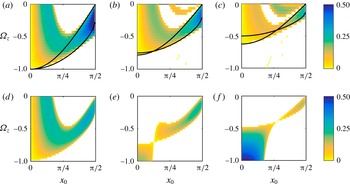
Figure 11. Colour plot of (a–c)
 ${\it\sigma}_{N}$
and (d–f)
${\it\sigma}_{N}$
and (d–f)
 ${\it\sigma}_{\unicode[STIX]{x1D63E}}^{\ast }$
as a function of
${\it\sigma}_{\unicode[STIX]{x1D63E}}^{\ast }$
as a function of
 $x_{0}$
and
$x_{0}$
and
 ${\it\Omega}_{z}$
for Taylor–Green vortices with (a,d)
${\it\Omega}_{z}$
for Taylor–Green vortices with (a,d)
 $E=1$
, (b,e)
$E=1$
, (b,e)
 $E=0.75$
and (c,f)
$E=0.75$
and (c,f)
 $E=0.5$
. White regions in the plots correspond to
$E=0.5$
. White regions in the plots correspond to
 $\text{Re}[{\it\sigma}_{N},{\it\sigma}_{\unicode[STIX]{x1D63E}}^{\ast }]\leqslant 0$
. All the plots correspond to
$\text{Re}[{\it\sigma}_{N},{\it\sigma}_{\unicode[STIX]{x1D63E}}^{\ast }]\leqslant 0$
. All the plots correspond to
 ${\it\tau}=0.3$
. The solid black curves in (a–c) show the
${\it\tau}=0.3$
. The solid black curves in (a–c) show the
 $-|{\it\Omega}_{z}|_{L,\unicode[STIX]{x1D63E}}$
versus
$-|{\it\Omega}_{z}|_{L,\unicode[STIX]{x1D63E}}$
versus
 $x_{0}$
and
$x_{0}$
and
 $-|{\it\Omega}_{z}|_{U,\unicode[STIX]{x1D63E}}$
versus
$-|{\it\Omega}_{z}|_{U,\unicode[STIX]{x1D63E}}$
versus
 $x_{0}$
variations, as described by (4.2) and (4.3).
$x_{0}$
variations, as described by (4.2) and (4.3).
For
 $E=0.75$
, a new smaller domain of instability emerges close to
$E=0.75$
, a new smaller domain of instability emerges close to
 ${\it\Omega}_{z}=0$
in the
${\it\Omega}_{z}=0$
in the
 ${\it\sigma}_{N}$
distribution (figure 11
b), whereas
${\it\sigma}_{N}$
distribution (figure 11
b), whereas
 ${\it\sigma}_{\unicode[STIX]{x1D63E}}^{\ast }$
does not pick up this new instability domain (figure 11
e). While
${\it\sigma}_{\unicode[STIX]{x1D63E}}^{\ast }$
does not pick up this new instability domain (figure 11
e). While
 ${\it\sigma}_{\unicode[STIX]{x1D63E}}^{\ast }$
captures the centrifugal instability for
${\it\sigma}_{\unicode[STIX]{x1D63E}}^{\ast }$
captures the centrifugal instability for
 $x_{0}\gtrsim 0.51$
, it does not predict the instability present in the region
$x_{0}\gtrsim 0.51$
, it does not predict the instability present in the region
 $x_{0}\lesssim 0.51,{\it\Omega}_{z}\geqslant -0.7$
and wrongly predicts instability for
$x_{0}\lesssim 0.51,{\it\Omega}_{z}\geqslant -0.7$
and wrongly predicts instability for
 $x_{0}\leqslant 0.39,{\it\Omega}_{z}\leqslant -0.707$
. The comparison between
$x_{0}\leqslant 0.39,{\it\Omega}_{z}\leqslant -0.707$
. The comparison between
 ${\it\sigma}_{N}$
and
${\it\sigma}_{N}$
and
 ${\it\sigma}_{\unicode[STIX]{x1D63E}}^{\ast }$
for
${\it\sigma}_{\unicode[STIX]{x1D63E}}^{\ast }$
for
 $E=0.5$
is qualitatively similar to that of
$E=0.5$
is qualitatively similar to that of
 $E=0.75$
, albeit with a larger domain for which
$E=0.75$
, albeit with a larger domain for which
 ${\it\sigma}_{\unicode[STIX]{x1D63E}}^{\ast }$
wrongly predicts instability. Upon increasing the axial velocity parameter
${\it\sigma}_{\unicode[STIX]{x1D63E}}^{\ast }$
wrongly predicts instability. Upon increasing the axial velocity parameter
 ${\it\tau}$
to 1.0 (figure 12), we observe an improvement in the agreement between
${\it\tau}$
to 1.0 (figure 12), we observe an improvement in the agreement between
 ${\it\sigma}_{\unicode[STIX]{x1D63E}}^{\ast }$
and
${\it\sigma}_{\unicode[STIX]{x1D63E}}^{\ast }$
and
 ${\it\sigma}_{N}$
. Specifically, the existence of two separate bands of unstable streamlines for a fixed
${\it\sigma}_{N}$
. Specifically, the existence of two separate bands of unstable streamlines for a fixed
 ${\it\Omega}_{z}$
is predicted by
${\it\Omega}_{z}$
is predicted by
 ${\it\sigma}_{\unicode[STIX]{x1D63E}}^{\ast }$
for
${\it\sigma}_{\unicode[STIX]{x1D63E}}^{\ast }$
for
 $E=1$
and
$E=1$
and
 $E=0.75$
.
$E=0.75$
.

Figure 12. Colour plot of (a–c)
 ${\it\sigma}_{N}$
and (d–f)
${\it\sigma}_{N}$
and (d–f)
 ${\it\sigma}_{\unicode[STIX]{x1D63E}}^{\ast }$
as a function of
${\it\sigma}_{\unicode[STIX]{x1D63E}}^{\ast }$
as a function of
 $x_{0}$
and
$x_{0}$
and
 ${\it\Omega}_{z}$
for Taylor–Green vortices with (a,d)
${\it\Omega}_{z}$
for Taylor–Green vortices with (a,d)
 $E=1$
, (b,e)
$E=1$
, (b,e)
 $E=0.75$
and (c,f)
$E=0.75$
and (c,f)
 $E=0.5$
. White regions in the plots correspond to
$E=0.5$
. White regions in the plots correspond to
 $\text{Re}[{\it\sigma}_{N},{\it\sigma}_{\unicode[STIX]{x1D63E}}^{\ast }]\leqslant 0$
. All the plots correspond to
$\text{Re}[{\it\sigma}_{N},{\it\sigma}_{\unicode[STIX]{x1D63E}}^{\ast }]\leqslant 0$
. All the plots correspond to
 ${\it\tau}=1.0$
. The solid black curves in (a–c) show the
${\it\tau}=1.0$
. The solid black curves in (a–c) show the
 $-|{\it\Omega}_{z}|_{L,\unicode[STIX]{x1D63E}}$
versus
$-|{\it\Omega}_{z}|_{L,\unicode[STIX]{x1D63E}}$
versus
 $x_{0}$
and
$x_{0}$
and
 $-|{\it\Omega}_{z}|_{U,\unicode[STIX]{x1D63E}}$
versus
$-|{\it\Omega}_{z}|_{U,\unicode[STIX]{x1D63E}}$
versus
 $x_{0}$
variations, as described by (4.2) and (4.3).
$x_{0}$
variations, as described by (4.2) and (4.3).
Similar to the thresholds introduced in the discussion of figure 8 for
 ${\it\tau}=0$
, we define corresponding
${\it\tau}=0$
, we define corresponding
 $|{\it\Omega}_{z}|_{L,N}$
and
$|{\it\Omega}_{z}|_{L,N}$
and
 $|{\it\Omega}_{z}|_{U,N}$
for the centrifugal instability domains for each
$|{\it\Omega}_{z}|_{U,N}$
for the centrifugal instability domains for each
 $x_{0}$
in figures 11(a–c) and 12(a–c). The lower threshold
$x_{0}$
in figures 11(a–c) and 12(a–c). The lower threshold
 $|{\it\Omega}_{z}|_{L,N}$
for streamlines with
$|{\it\Omega}_{z}|_{L,N}$
for streamlines with
 $x_{0}\leqslant 0.55$
is zero for
$x_{0}\leqslant 0.55$
is zero for
 ${\it\tau}=0.3$
and
${\it\tau}=0.3$
and
 $E=1$
(figure 11
a). The corresponding range of streamlines for which
$E=1$
(figure 11
a). The corresponding range of streamlines for which
 $|{\it\Omega}_{z}|_{L,N}=0$
at
$|{\it\Omega}_{z}|_{L,N}=0$
at
 ${\it\tau}=0.3$
are
${\it\tau}=0.3$
are
 $x_{0}\leqslant 0.5$
and
$x_{0}\leqslant 0.5$
and
 $x_{0}\leqslant 0.46$
for
$x_{0}\leqslant 0.46$
for
 $E=0.75$
and
$E=0.75$
and
 $E=0.5$
, respectively. With a further increase in
$E=0.5$
, respectively. With a further increase in
 ${\it\tau}$
to 1, the range of streamlines with
${\it\tau}$
to 1, the range of streamlines with
 $|{\it\Omega}_{z}|_{L,N}=0$
spreads to larger values of
$|{\it\Omega}_{z}|_{L,N}=0$
spreads to larger values of
 $x_{0}$
. For a small range of streamlines close to the edge of the vortex,
$x_{0}$
. For a small range of streamlines close to the edge of the vortex,
 $|{\it\Omega}_{z}|_{L,N}$
is invariant with
$|{\it\Omega}_{z}|_{L,N}$
is invariant with
 ${\it\tau}$
for
${\it\tau}$
for
 ${\it\tau}\leqslant 1$
.
${\it\tau}\leqslant 1$
.
For each of
 $E=1,0.75$
and 0.5, the variation of
$E=1,0.75$
and 0.5, the variation of
 $|{\it\Omega}_{z}|_{U,N}$
as a function of
$|{\it\Omega}_{z}|_{U,N}$
as a function of
 $x_{0}$
is independent of
$x_{0}$
is independent of
 ${\it\tau}$
. Recalling that the threshold
${\it\tau}$
. Recalling that the threshold
 $|{\it\Omega}_{z}|_{2,N}$
corresponds to
$|{\it\Omega}_{z}|_{2,N}$
corresponds to
 $\mathit{Ro}=1$
for all
$\mathit{Ro}=1$
for all
 $E$
in figure 6, we conclude that the criterion
$E$
in figure 6, we conclude that the criterion
 $\mathit{Ro}<1$
for centrifugal stability in anticyclonic Taylor–Green vortices is independent of
$\mathit{Ro}<1$
for centrifugal stability in anticyclonic Taylor–Green vortices is independent of
 $E$
and
$E$
and
 ${\it\tau}$
for
${\it\tau}$
for
 ${\it\tau}\leqslant 1$
. The significance of the solid black curves in figures 11(a–c) and 12(a–c), which capture the upper threshold
${\it\tau}\leqslant 1$
. The significance of the solid black curves in figures 11(a–c) and 12(a–c), which capture the upper threshold
 $|{\it\Omega}_{z}|_{U,N}$
well, is discussed in § 4.
$|{\it\Omega}_{z}|_{U,N}$
well, is discussed in § 4.
4. Discussion and conclusions
In this paper, we derived a criterion for centrifugal instability in an axisymmetric vortex with axial flow and background rotation. The criterion was then heuristically extended to non-axisymmetric vortices. The resulting non-axisymmetric criterion (2.10), which converges to the criterion of Bayly (Reference Bayly1988) in the absence of background rotation and axial flow, was then evaluated for two different vortex models: the Stuart vortices and the Taylor–Green vortices. For Taylor–Green vortices with no background rotation and large axial flow,
 ${\it\sigma}_{\unicode[STIX]{x1D63E}}^{\ast }$
is shown to be reasonably accurate for streamlines satisfying
${\it\sigma}_{\unicode[STIX]{x1D63E}}^{\ast }$
is shown to be reasonably accurate for streamlines satisfying
 $S\lesssim 0.2$
, with
$S\lesssim 0.2$
, with
 $S$
being the extent of non-axisymmetry. An investigation of how the threshold axial flow, beyond which centrifugal instability emerges in Taylor–Green vortices with no background rotation, varies as a function of
$S$
being the extent of non-axisymmetry. An investigation of how the threshold axial flow, beyond which centrifugal instability emerges in Taylor–Green vortices with no background rotation, varies as a function of
 $x_{0}$
and
$x_{0}$
and
 $E$
would be worthwhile.
$E$
would be worthwhile.
For Stuart and Taylor–Green vortices without an axial flow, the criterion (2.10) based on
 ${\it\sigma}_{\unicode[STIX]{x1D63E}}^{\ast }$
performs remarkably well in delineating the stable and unstable regions in the
${\it\sigma}_{\unicode[STIX]{x1D63E}}^{\ast }$
performs remarkably well in delineating the stable and unstable regions in the
 ${\it\rho}$
–
${\it\rho}$
–
 ${\it\Omega}_{z}$
and
${\it\Omega}_{z}$
and
 $E$
–
$E$
–
 ${\it\Omega}_{z}$
planes, respectively. This criterion is also shown to perform qualitatively and quantitatively better than the sufficient criterion proposed by Sipp & Jacquin (Reference Sipp and Jacquin2000). In the presence of both axial flow and background rotation, our criterion accurately predicts the range of centrifugally unstable streamlines and their growth rates for sufficiently large values of
${\it\Omega}_{z}$
planes, respectively. This criterion is also shown to perform qualitatively and quantitatively better than the sufficient criterion proposed by Sipp & Jacquin (Reference Sipp and Jacquin2000). In the presence of both axial flow and background rotation, our criterion accurately predicts the range of centrifugally unstable streamlines and their growth rates for sufficiently large values of
 ${\it\rho}$
and
${\it\rho}$
and
 $E$
.
$E$
.
We now explain some of the numerical results in § 3 using the criterion in (2.10). In the absence of an axial flow, the criterion for instability in (2.10) reduces to
 $$\begin{eqnarray}-({\it\sigma}_{\unicode[STIX]{x1D63E}\{1,2\}}^{\ast })^{2}=\left(\frac{4{\rm\pi}}{T}+2{\it\Omega}_{z}\right)\left(\frac{1}{T}\frac{\text{d}{\it\Gamma}}{\text{d}{\it\psi}}+2{\it\Omega}_{z}\right)<0,\end{eqnarray}$$
as already shown in (3.5). Restricting our analysis to streamlines in vortices for which
 $T$
and
$T$
and
 $\text{d}{\it\Gamma}/\text{d}{\it\psi}$
are both positive, we consider the variation of
$\text{d}{\it\Gamma}/\text{d}{\it\psi}$
are both positive, we consider the variation of
 $({\it\sigma}_{\unicode[STIX]{x1D63E}\{1,2\}}^{\ast })^{2}$
with
$({\it\sigma}_{\unicode[STIX]{x1D63E}\{1,2\}}^{\ast })^{2}$
with
 ${\it\Omega}_{z}$
. At
${\it\Omega}_{z}$
. At
 ${\it\Omega}_{z}=0$
, the criterion in (4.1) is not satisfied, and the corresponding streamline is centrifugally stable. As
${\it\Omega}_{z}=0$
, the criterion in (4.1) is not satisfied, and the corresponding streamline is centrifugally stable. As
 ${\it\Omega}_{z}$
is decreased from zero,
${\it\Omega}_{z}$
is decreased from zero,
 $({\it\sigma}_{\unicode[STIX]{x1D63E}\{1,2\}}^{\ast })^{2}$
becomes positive first at
$({\it\sigma}_{\unicode[STIX]{x1D63E}\{1,2\}}^{\ast })^{2}$
becomes positive first at
 ${\it\Omega}_{z}=(-1/2T)\min (4{\rm\pi},\text{d}{\it\Gamma}/\text{d}{\it\psi})$
. For every streamline in figures 5(b,e) and 8(d–f), the threshold
${\it\Omega}_{z}=(-1/2T)\min (4{\rm\pi},\text{d}{\it\Gamma}/\text{d}{\it\psi})$
. For every streamline in figures 5(b,e) and 8(d–f), the threshold
 $|{\it\Omega}_{z}|_{L,\unicode[STIX]{x1D63E}}$
is therefore given by
$|{\it\Omega}_{z}|_{L,\unicode[STIX]{x1D63E}}$
is therefore given by
 $$\begin{eqnarray}|{\it\Omega}_{z}|_{L,\unicode[STIX]{x1D63E}}=(1/2T)\min (4{\rm\pi},\text{d}{\it\Gamma}/\text{d}{\it\psi}),\end{eqnarray}$$
with the
 $\unicode[STIX]{x1D63E}$
in the subscript referring to the criterion in (4.1). The above threshold is an estimate of the threshold
$\unicode[STIX]{x1D63E}$
in the subscript referring to the criterion in (4.1). The above threshold is an estimate of the threshold
 $|{\it\Omega}_{z}|_{L,N}$
found in the corresponding
$|{\it\Omega}_{z}|_{L,N}$
found in the corresponding
 ${\it\sigma}_{N}$
distributions. The outermost streamline in both Stuart (
${\it\sigma}_{N}$
distributions. The outermost streamline in both Stuart (
 $x_{0}={\rm\pi}$
) and Taylor–Green (
$x_{0}={\rm\pi}$
) and Taylor–Green (
 $x_{0}={\rm\pi}/2$
) vortices corresponds to
$x_{0}={\rm\pi}/2$
) vortices corresponds to
 $T\rightarrow \infty$
, thus resulting in
$T\rightarrow \infty$
, thus resulting in
 $|{\it\Omega}_{z}|_{L,\unicode[STIX]{x1D63E}}=0$
based on (4.2).
$|{\it\Omega}_{z}|_{L,\unicode[STIX]{x1D63E}}=0$
based on (4.2).
Upon increasing
 $|{\it\Omega}_{z}|$
further beyond
$|{\it\Omega}_{z}|$
further beyond
 $|{\it\Omega}_{z}|_{L,\unicode[STIX]{x1D63E}}$
for a given streamline,
$|{\it\Omega}_{z}|_{L,\unicode[STIX]{x1D63E}}$
for a given streamline,
 $({\it\sigma}_{\unicode[STIX]{x1D63E}\{1,2\}}^{\ast })^{2}$
becomes negative again at
$({\it\sigma}_{\unicode[STIX]{x1D63E}\{1,2\}}^{\ast })^{2}$
becomes negative again at
 $$\begin{eqnarray}|{\it\Omega}_{z}|_{U,\unicode[STIX]{x1D63E}}=(1/2T)\max (4{\rm\pi},\text{d}{\it\Gamma}/\text{d}{\it\psi}),\end{eqnarray}$$
which is an estimate of the threshold
 $|{\it\Omega}_{z}|_{U,N}$
above which the streamline becomes centrifugally stable based on
$|{\it\Omega}_{z}|_{U,N}$
above which the streamline becomes centrifugally stable based on
 ${\it\sigma}_{N}$
.
${\it\sigma}_{N}$
.
In Stuart vortices with no axial flow (
 ${\it\tau}=0$
),
${\it\tau}=0$
),
 $|{\it\Omega}_{z}|_{L,\unicode[STIX]{x1D63E}}$
and
$|{\it\Omega}_{z}|_{L,\unicode[STIX]{x1D63E}}$
and
 $|{\it\Omega}_{z}|_{U,\unicode[STIX]{x1D63E}}$
accurately capture the centrifugally unstable domain on the
$|{\it\Omega}_{z}|_{U,\unicode[STIX]{x1D63E}}$
accurately capture the centrifugally unstable domain on the
 $\tilde{{\it\psi}}$
–
$\tilde{{\it\psi}}$
–
 ${\it\Omega}_{z}$
plane for both
${\it\Omega}_{z}$
plane for both
 ${\it\rho}=0.745$
(solid black curves in figure 5
a) and
${\it\rho}=0.745$
(solid black curves in figure 5
a) and
 ${\it\rho}=0.602$
(solid black curves in figure 5
d). We recall that the maximum of
${\it\rho}=0.602$
(solid black curves in figure 5
d). We recall that the maximum of
 $|{\it\Omega}_{z}|_{U,\unicode[STIX]{x1D63E}}$
among all the streamlines for a given
$|{\it\Omega}_{z}|_{U,\unicode[STIX]{x1D63E}}$
among all the streamlines for a given
 ${\it\rho}$
represents the threshold
${\it\rho}$
represents the threshold
 $|{\it\Omega}_{z}|_{2,\unicode[STIX]{x1D63E}}$
plotted in figure 3.
$|{\it\Omega}_{z}|_{2,\unicode[STIX]{x1D63E}}$
plotted in figure 3.
In the presence of an axial flow, the upper threshold estimate
 $|{\it\Omega}_{z}|_{U,\unicode[STIX]{x1D63E}}$
in (4.3) remains remarkably accurate in predicting the maximum magnitude of rotation above which streamlines in the Stuart vortices with
$|{\it\Omega}_{z}|_{U,\unicode[STIX]{x1D63E}}$
in (4.3) remains remarkably accurate in predicting the maximum magnitude of rotation above which streamlines in the Stuart vortices with
 ${\it\rho}=0.9$
and
${\it\rho}=0.9$
and
 ${\it\rho}=0.745$
become centrifugally stable (the bottom solid black curves in figures 9
a,b and 10
a,b). The lower threshold
${\it\rho}=0.745$
become centrifugally stable (the bottom solid black curves in figures 9
a,b and 10
a,b). The lower threshold
 $|{\it\Omega}_{z}|_{L,\unicode[STIX]{x1D63E}}$
, however, does not capture the centrifugal instability induced by the axial flow effects in the streamlines around the origin.
$|{\it\Omega}_{z}|_{L,\unicode[STIX]{x1D63E}}$
, however, does not capture the centrifugal instability induced by the axial flow effects in the streamlines around the origin.
In Taylor–Green vortices,
 $|{\it\Omega}_{z}|_{L,\unicode[STIX]{x1D63E}}$
is accurate in describing the lower threshold for
$|{\it\Omega}_{z}|_{L,\unicode[STIX]{x1D63E}}$
is accurate in describing the lower threshold for
 ${\it\tau}=0$
(figure 8
a–c) whereas
${\it\tau}=0$
(figure 8
a–c) whereas
 $|{\it\Omega}_{z}|_{U,\unicode[STIX]{x1D63E}}$
remains accurate even in the presence of axial flow (figures 8
a–c, 11
a–c and 12
a–c). In summary,
$|{\it\Omega}_{z}|_{U,\unicode[STIX]{x1D63E}}$
remains accurate even in the presence of axial flow (figures 8
a–c, 11
a–c and 12
a–c). In summary,
 $|{\it\Omega}_{z}|_{U,\unicode[STIX]{x1D63E}}$
represents a reasonably accurate estimate of
$|{\it\Omega}_{z}|_{U,\unicode[STIX]{x1D63E}}$
represents a reasonably accurate estimate of
 $|{\it\Omega}_{z}|_{U,N}$
for both Stuart and Taylor–Green vortices with
$|{\it\Omega}_{z}|_{U,N}$
for both Stuart and Taylor–Green vortices with
 ${\it\tau}\leqslant 1$
, and hence its maximum among all streamlines represents an estimate of
${\it\tau}\leqslant 1$
, and hence its maximum among all streamlines represents an estimate of
 $|{\it\Omega}_{z}|_{2,N}$
beyond which the vortex with a specific value of
$|{\it\Omega}_{z}|_{2,N}$
beyond which the vortex with a specific value of
 ${\it\rho}$
or
${\it\rho}$
or
 $E$
is centrifugally stable.
$E$
is centrifugally stable.
An interesting observation based on figures 9(f), 10(f), 11(e,f) and 12(e,f) is that
 ${\it\sigma}_{\unicode[STIX]{x1D63E}}^{\ast }$
fails to predict the instability for
${\it\sigma}_{\unicode[STIX]{x1D63E}}^{\ast }$
fails to predict the instability for
 $|{\it\Omega}_{z}|<|{\it\Omega}_{z}|_{L,\unicode[STIX]{x1D63E}}$
, and wrongly predicts instability well above
$|{\it\Omega}_{z}|<|{\it\Omega}_{z}|_{L,\unicode[STIX]{x1D63E}}$
, and wrongly predicts instability well above
 $|{\it\Omega}_{z}|=|{\it\Omega}_{z}|_{L,\unicode[STIX]{x1D63E}}$
for a range of streamlines around the origin. This range of streamlines, for which
$|{\it\Omega}_{z}|=|{\it\Omega}_{z}|_{L,\unicode[STIX]{x1D63E}}$
for a range of streamlines around the origin. This range of streamlines, for which
 ${\it\sigma}_{\unicode[STIX]{x1D63E}}^{\ast }$
fails, coincides with the region to the left of the point of intersection between the
${\it\sigma}_{\unicode[STIX]{x1D63E}}^{\ast }$
fails, coincides with the region to the left of the point of intersection between the
 $|{\it\Omega}_{z}|_{L,\unicode[STIX]{x1D63E}}$
and
$|{\it\Omega}_{z}|_{L,\unicode[STIX]{x1D63E}}$
and
 $|{\it\Omega}_{z}|_{U,\unicode[STIX]{x1D63E}}$
curves plotted in the corresponding
$|{\it\Omega}_{z}|_{U,\unicode[STIX]{x1D63E}}$
curves plotted in the corresponding
 ${\it\sigma}_{N}$
figures. The point of intersection between
${\it\sigma}_{N}$
figures. The point of intersection between
 $|{\it\Omega}_{z}|_{L,\unicode[STIX]{x1D63E}}$
and
$|{\it\Omega}_{z}|_{L,\unicode[STIX]{x1D63E}}$
and
 $|{\it\Omega}_{z}|_{U,\unicode[STIX]{x1D63E}}$
occurs at
$|{\it\Omega}_{z}|_{U,\unicode[STIX]{x1D63E}}$
occurs at
 $\text{d}{\it\Gamma}/\text{d}{\it\psi}=4{\rm\pi}$
, and the criterion based on
$\text{d}{\it\Gamma}/\text{d}{\it\psi}=4{\rm\pi}$
, and the criterion based on
 ${\it\sigma}_{\unicode[STIX]{x1D63E}}^{\ast }$
(2.10) is therefore observed to fail on streamlines with
${\it\sigma}_{\unicode[STIX]{x1D63E}}^{\ast }$
(2.10) is therefore observed to fail on streamlines with
 $\text{d}{\it\Gamma}/\text{d}{\it\psi}>4{\rm\pi}$
in the presence of background rotation and/or axial flow.
$\text{d}{\it\Gamma}/\text{d}{\it\psi}>4{\rm\pi}$
in the presence of background rotation and/or axial flow.
In the case of cyclonic rotation, i.e.
 ${\it\Omega}_{z}>0$
, the criterion in (4.1) is not satisfied for all
${\it\Omega}_{z}>0$
, the criterion in (4.1) is not satisfied for all
 ${\it\Omega}_{z}$
if
${\it\Omega}_{z}$
if
 $T>0$
and
$T>0$
and
 $\text{d}{\it\Gamma}/\text{d}{\it\psi}>0$
. Therefore, a centrifugally stable vortex (with no axial flow and background rotation) remains centrifugally stable with the addition of cyclonic rotation, a result consistent with the results of Sipp et al. (Reference Sipp, Lauga and Jacquin1999). It would furthermore be worthwhile to investigate the validity of (2.10) in describing centrifugal instability in vortices that are centrifugally unstable even without axial flow and background rotation.
$\text{d}{\it\Gamma}/\text{d}{\it\psi}>0$
. Therefore, a centrifugally stable vortex (with no axial flow and background rotation) remains centrifugally stable with the addition of cyclonic rotation, a result consistent with the results of Sipp et al. (Reference Sipp, Lauga and Jacquin1999). It would furthermore be worthwhile to investigate the validity of (2.10) in describing centrifugal instability in vortices that are centrifugally unstable even without axial flow and background rotation.
The heuristic transformation from the axisymmetric to non-axisymmetric criterion presented in § 2 is not unique, and other ways of expressing criterion (2.8) in terms of
 ${\it\Gamma}$
and
${\it\Gamma}$
and
 $T$
could be explored. For example, the denominator of the first term in criterion (2.8) could also be rewritten to give
$T$
could be explored. For example, the denominator of the first term in criterion (2.8) could also be rewritten to give
 $$\begin{eqnarray}\displaystyle ({\it\sigma}_{\unicode[STIX]{x1D63E}\{1,2\}}^{\ast })^{2} & = & \displaystyle \left[\frac{4(\text{d}w/\text{d}{\it\psi})^{2}({\it\Omega}_{z}+{\it\psi}^{\prime }/r)^{2}}{(1/r^{2})(\text{d}(r{\it\psi}^{\prime })/\text{d}{\it\psi}-2)^{2}+(\text{d}w/\text{d}{\it\psi})^{2}}\right.\nonumber\\ \displaystyle & & \displaystyle \left.-\,2\left(\frac{{\it\psi}^{\prime }}{r}+{\it\Omega}_{z}\right)\left(\frac{{\it\psi}^{\prime }}{r}\frac{\text{d}(r{\it\psi}^{\prime })}{\text{d}{\it\psi}}+2{\it\Omega}_{z}\right)\right]>0,\end{eqnarray}$$
which would then not involve
 $\text{d}T/\text{d}{\it\psi}$
when
$\text{d}T/\text{d}{\it\psi}$
when
 ${\it\psi}^{\prime }$
and
${\it\psi}^{\prime }$
and
 $r$
are written in terms of
$r$
are written in terms of
 ${\it\Gamma}$
and
${\it\Gamma}$
and
 $T$
. It would be interesting to evaluate the accuracy of the resulting criterion, which would still converge to the exact criterion of Bayly (Reference Bayly1988) for
$T$
. It would be interesting to evaluate the accuracy of the resulting criterion, which would still converge to the exact criterion of Bayly (Reference Bayly1988) for
 ${\it\Omega}_{z}=0$
and
${\it\Omega}_{z}=0$
and
 ${\it\tau}=0$
, in describing centrifugal instability in non-axisymmetric vortices. An exact analytical criterion to describe centrifugal instability in arbitrarily non-axisymmetric vortices remains elusive.
${\it\tau}=0$
, in describing centrifugal instability in non-axisymmetric vortices. An exact analytical criterion to describe centrifugal instability in arbitrarily non-axisymmetric vortices remains elusive.
Acknowledgements
We thank J.-M. Chomaz for suggesting the form of figure 3. We also thank the anonymous referees for their comments which helped improve the paper.


