3.1. Modification of the Betz analysis

The Betz analysis proceeds by equating the horizontal force on an actuator disk representing the turbine multiplied by the horizontal velocity through the disk, with the power extracted by the turbine. Accordingly the vertical and cross-stream components of the momentum equation play no role in the analysis, and only the horizontal (streamwise) component of the momentum equation is of interest. The analysis in § 3.1 again largely follows that in Young et al. (Reference Young, Tian and Lai2017), but with important additional physics considered (work by viscous forces and viscous dissipation as noted above, and fluctuating forces on the turbine plane as discussed below). The horizontal component of (2.10), and (2.11) are rewritten as

(3.1)\begin{gather} {F_x} = -\int_{CS} \rho U U_j n_j \, \textrm{d} A + C_{\alpha}\tfrac{1}{2}\dot{m}U_{\infty} = \tfrac{1}{2}\dot{m}U_{\infty} (C_{FM}+C_{\alpha}), \end{gather}

(3.2)\begin{gather}\overline{\dot{W}} = -\int_{CS}\tfrac{1}{2}\rho U_i U_i U_j n_j \, \textrm{d} A + C_{\beta}\tfrac{1}{2}\dot{m}U_{\infty}^2 = \tfrac{1}{2}\dot{m}U_{\infty}^2(C_{WKE}+C_{\beta}), \end{gather}

where $C_{FM}$ and $C_{WKE}$ encompass respectively the time-average horizontal momentum and the time-average kinetic energy entering and leaving the control volume. Note the omission of subscript for the first $U$ in (3.1), indicating this is the horizontal velocity component only; $C_{\alpha }$ and $C_{\beta }$ encapsulate the effects ignored in the standard Betz analysis, including non-free-stream pressure on the control surface boundary, viscous effects and unsteady flow effects, with each of these defined in coefficient form below:

(3.3)\begin{gather} \left.\begin{array}{c@{}} C_{FM} = -\displaystyle\dfrac{1}{\frac{1}{2}\dot{m}U_{\infty}} \int_{CS}\rho U U_j n_j \, \textrm{d} A \\ C_{WKE} = -\displaystyle\dfrac{1}{\frac{1}{2}\dot{m}U_{\infty}^2} \int_{CS}\frac{1}{2}\rho U_i U_i U_j n_j \, \textrm{d} A \\ \end{array}\right\}, \end{gather}

(3.4)\begin{gather}C_{\alpha} = C_{FP} + C_{FV} + C_{FR}, \end{gather}

(3.5)\begin{gather}C_{\beta} = C_{WPA} + C_{WPF} + C_{WA} + C_{WB} + C_{WC}, \end{gather}

(3.6)\begin{gather}\left.\begin{array}{c@{}} C_{FP} = -\displaystyle\dfrac{1}{\frac{1}{2}\dot{m}U_{\infty}} \int_{CS}P n_x \, \textrm{d} A \\ C_{FV} = \displaystyle\dfrac{1}{\frac{1}{2}\dot{m}U_{\infty}} \int_{CS} \bar{\tau}_{xj} n_j \, \textrm{d} A \\ C_{FR} = -\displaystyle\dfrac{1}{\frac{1}{2}\dot{m}U_{\infty}} \int_{CS}\rho \overline{u' u'_j} n_j \, \textrm{d} A \\ C_{WPA} = -\displaystyle\dfrac{1}{\frac{1}{2}\dot{m}U_{\infty}^2} \int_{CS}PU_j n_j \, \textrm{d} A \\ C_{WPF} = -\displaystyle\dfrac{1}{\frac{1}{2}\dot{m}U_{\infty}^2} \int_{CS}\overline{p'u'_j} n_j \, \textrm{d} A \\ C_{WA} = -\displaystyle\dfrac{1}{\frac{1}{2}\dot{m}U_{\infty}^2} \int_{CS} \frac{1}{2}\rho (\overline{u'_i u'_i}U_j +2 U_i \overline{u'_i u'_j}+ \overline{u'_i u'_i u'_j} ) n_j \, \textrm{d} A \\ C_{WB} = \displaystyle\dfrac{1}{\frac{1}{2}\dot{m}U_{\infty}^2} \int_{CS} \overline{u_i \tau_{ij}} n_j \, \textrm{d} A \\ C_{WC} = -\displaystyle\dfrac{1}{\frac{1}{2}\dot{m}U_{\infty}^2} \int_{CV} \bar{\phi} \, \textrm{d} V \end{array}\right\}. \end{gather}

Note again the use of the $x$ subscript ($n_x$ in $C_{FP}$ and $\bar {\tau }_{xj}$ in $C_{FV}$), and the lack of subscript for the first $u'$ in $C_{FR}$, as these coefficients are based on horizontal (i.e. streamwise) components of force. The additional terms representing momentum ($C_{\alpha }$) and energy ($C_{\beta }$) flows in and out of the control volume provide a mechanism by which the energy extraction and efficiency of the turbine may be altered, by modifying the pressure drop across (and hence force on) the turbine plane, or the average flow velocity through the turbine plane or both, either separately or together.

We take the usual step of equating the power extracted by the turbine $\dot {W}$, with the vector multiplication of the force $f_i$ on the turbine and the velocity through the turbine plane $u_{T_i}=U_{T_i}+u'_{T_i}$. Unlike the standard Betz analysis we must take into account that the force and velocity are fluctuating quantities, and we must also include dissipation and any other losses of mechanical energy across the turbine plane $\dot {W}_{LT}$. At this point $\dot {W}_{LT}$ is included as a necessary term, and its evaluation is discussed in § 3.3.

(3.7)\begin{equation} \left.\begin{array}{c@{}} \dot{W} = f_i u_{T_i} - \dot{W}_{LT}\\ \overline{\dot{W}} = F_i U_{T_i} + \overline{f'_i u'_{T_i}} - \overline{\dot{W}}_{LT} = F_x U_{T} + \overline{f'_i u'_{T_i}} - \overline{\dot{W}}_{LT} \end{array}\right\}.\end{equation}

Here the time-averaged values of forces on the turbine and velocities through the turbine plane are zero in all directions except streamwise due to symmetry. Noting that mass flow rate $\dot {m}=\rho U_{\infty } A_1=\rho U_T A_T$ and having used (3.7) to solve for $U_{T}$, the efficiency of power extraction is then

(3.8)\begin{equation} \eta = \frac{\overline{\dot{W}}}{\frac{1}{2}\rho U_{\infty}^3 A_T} = \frac{1}{\frac{1}{2}\dot{m}U_{\infty}^3}\frac{\overline{\dot{W}}}{{F_x}}(\overline{\dot{W}} - \overline{f'_i u'_{T_i}} + \overline{\dot{W}}_{LT}), \end{equation}

with the efficiency being related to the mean output power coefficient via

(3.9)\begin{equation} \bar{C}_P = \frac{\overline{\dot{W}}}{\frac{1}{2}\rho U_{\infty}^3 A_F} = \eta \frac{A_T}{A_F},\end{equation}

where $A_F$ is the planform area of the foil. For a rectangular foil this reduces to $\bar {C}_P = \eta d/c$ where $c$ is the foil chord and $d$ is the vertical distance swept by the trailing edge.

We define one further coefficient

(3.10)\begin{equation} C_{\gamma} = \frac{- \overline{f'_i u'_{T_i}} + \overline{\dot{W}}_{LT} }{\frac{1}{2}\dot{m}U_{\infty}^2},\end{equation}

which encapsulates the fluctuating force and velocity terms and losses of mechanical energy across the turbine plane. Using (3.1)–(3.6) and (3.10), the efficiency reduces to

(3.11)\begin{equation} \eta = \frac{(C_{WKE}+C_{\beta})(C_{WKE}+C_{\beta}+C_{\gamma})}{C_{FM}+C_{\alpha}}.\end{equation}

We now perform the integrations over the control surface in (3.3), noting that the only places where the time-averaged velocity is not orthogonal to the local outward normal are the inlet and exit. This gives an efficiency of

(3.12)\begin{equation} \eta = \frac{(1-a^2+C_{\beta})(1-a^2+C_{\beta}+C_{\gamma})}{2(1-a)+C_{\alpha}},\end{equation}

and a time-averaged velocity through the turbine plane of

(3.13)\begin{equation} \frac{U_T}{U_{\infty}} = \frac{\overline{\dot{W}}-\overline{f'_i u'_{T_i}}}{U_{\infty} {F_x}} = \frac{C_{WKE}+C_{\beta}+C_{\gamma}}{C_{FM}+C_{\alpha}} = \frac{1-a^2+C_{\beta}+C_{\gamma}}{2(1-a)+C_{\alpha}}, \end{equation}

using the definition $a = U_{E}/U_{\infty }$, the ratio of the far downstream wake and upstream velocities. The horizontal time-averaged velocity components at the CS inlet and exit, $U_{\infty }$ and $U_{E}$ are taken to be uniform across those boundaries, and the vertical components $V_1$ and $V_2$ are ignored as small relative to the horizontal components. These assumptions are examined in § 3.3. For comparison when only the mean momentum and energy terms are considered, as in the standard Betz analysis, the efficiency becomes the usual

(3.14)\begin{equation} \eta = \frac{(C_{WKE})^2}{C_{FM}} = \frac{(1-a^2)^2}{2(1-a)}.\end{equation}

Differentiating (3.12) with respect to $a$ and setting the result to zero to find the $a = a_{opt}$ value for maximum efficiency requires solution of a quartic equation in $a$.

(3.15)\begin{gather} a_{opt} = a : \frac{\partial \eta}{\partial a} = 0, \end{gather}

(3.16)\begin{gather}\eta_{max} =\frac{(1-a_{opt}^2+C_{\beta})(1-a_{opt}^2+C_{\beta}+C_{\gamma})}{2(1-a_{opt})+C_{\alpha}}. \end{gather}

This is done symbolically using the Matlab Symbolic Math Toolbox, which returns four roots. The correct physical one can be identified because setting $C_{\alpha } = C_{\beta } = C_{\gamma } = 0$ (indicating no unsteadiness, no mean pressure flow work, no viscous effects, etc.) recovers the usual Betz result of $a_{opt} = 1/3$, $U_T / U_{\infty } = 2/3$ and $\eta _{max} = 16/27$ for only one of the roots. The resulting expression for $a_{opt}$ is not provided here due to its length.

3.2. Performance limits from the modified Betz analysis

Equation (3.11) represents the actual efficiency achieved by the flapping foil turbine, which may be determined by calculating all the coefficients defined in (3.3)–(3.10). In contrast, (3.16) represents the maximum efficiency that the turbine could potentially achieve under the same conditions. In this section we determine the latter, while the following section evaluates the coefficients from numerical simulation to show whether this maximum performance could be achieved in practice.

Without knowing a priori physically realistic signs or magnitudes of $C_{\alpha }$, $C_{\beta }$ and $C_{\gamma }$, we can nevertheless determine that there exist numerical combinations of these coefficients that result in $\eta _{max} > 16/27$ in (3.16). A starting point to make the analysis tractable is to consider the effect of $C_{\alpha }$ and $C_{\beta }$ (momentum and energy fluxes), with $C_{\gamma }=0$. Applying constraints to ensure non-imaginary solutions for $\eta _{max}$, $0 < a_{opt} < 1$ (i.e. the downstream flow velocity remains both positive and less than the upstream velocity), and $\eta _{max} < 1$ (the turbine cannot extract more energy than exists in the flow) results in the region shown in figure 2, and the corresponding contours of turbine plane velocity $U_T / U_{\infty }$ in figure 3. Figure 2 suggests that in principle the Betz limit may be exceeded – the question then becomes whether these numerical values of $C_{\alpha }$, $C_{\beta }$ and $C_{\gamma }$ are physically realistic or indeed possible for the flapping foil turbine.

Figure 2. Region of $C_{\alpha }$ and $C_{\beta }$ space (shaded) for which $16/27 < \eta _{max} < 1$ and $0 < a_{opt} < 1$, from (3.15) and (3.16), with $C_{\gamma }=0$. Contours equally spaced between $\eta _{max} = 16/27$ and $\eta _{max} = 1$, adapted from Young et al. (Reference Young, Tian and Lai2017).

Figure 3. Contours of $U_T / U_{\infty }$ from (3.13), with $a = a_{opt}$ for all values of $C_{\alpha }$ and $C_{\beta }$, with $C_{\gamma }=0$. Shaded region as for figure 2.

For example, in figure 2 with $C_{\beta } = 0$, positive values of $C_{\alpha }$ reduce $\eta _{max}$, but $-0.268 < C_{\alpha } < 0$ results in $0.77 > \eta _{max} > 0.593$. This would require either the net force due to non-uniform pressure on the control surface to be negative (pressure at the downstream CS outlet higher than at the inlet, which is not physically realistic), or the viscous force on the sides of the CS to be negative (again not physically realistic given that the flow on the CS sides is in the downstream direction), or that there is a net transport of momentum out of the CS sides due to unsteady effects. Whether the latter is realistic is not immediately apparent, but is evaluated in § 3.3. Alternatively, leaving $C_{\alpha } = 0$, $\eta _{max} > 16/27$ for $0 < C_{\beta } < 0.25$. The $C_{WPA}$ component due to non-uniform pressure would be zero along the CS sides (no time-average flow across the boundary) but would be expected to be small and positive from contributions at the CS inlet and outlet since again $P_1 < P_2$ is not physically realistic. The expected sign and magnitude of the other terms comprising $C_{\beta }$ are harder to estimate without direct evaluation as in § 3.3. Figure 2 also shows values of $\eta _{max} > 16/27$ even where $C_{\beta } < 0$, i.e. where energy is being extracted from the control volume by unsteady effects and mean pressure flow work, rather than additional energy being provided. This is discussed further in § 3.4. Finally, one may note additional issues at the extremes of this analysis; for example at $C_{\alpha }=0$ and $C_{\beta }=0.25$, the predicted maximum efficiency is $\eta _{max}=1.0$ and yet $U_T / U_{\infty }=1.0$, thus the foil is extracting all the available power without creating any velocity change between the far upstream and the turbine plane. This comes about because we have imposed these given values of $C_{\alpha }$ and $C_{\beta }$, without accounting for how they would be or whether they could be produced, which is the focus of the next section.

Note that it is sufficient to consider the effect of $C_{\alpha }$, $C_{\beta }$ and $C_{\gamma }$ on the maximum efficiency $\eta _{max}$ alone, and not also on the mean power coefficient $\bar {C}_P$, due to the relationship between them in (3.9). For a given foil and kinematics, the foil area and turbine plane area are constants and the power coefficient differs from the efficiency only by a constant multiple.

It should also be noted that the analysis so far has made no assumption of the dimensionality of the control volume, so is equally applicable to two-dimensional (2-D) or 3-D flows. In what follows here for a single foil an evaluation of the pressure and velocity correlation terms has been made using 2-D simulations, as a demonstration of the methodology and to simplify the interpretation of the results. The impact of three-dimensionality is further discussed in § 4.2.

3.3. Evaluation of non-idealised momentum and energy terms

The 2-D unsteady viscous incompressible flow around a flapping foil was simulated with an in-house immersed-boundary lattice-Boltzmann method solver (Tian et al. Reference Tian, Luo, Zhu, Liao and Lu2011; Liu et al. Reference Liu, Lai, Young and Tian2017). The most efficient case from Kinsey & Dumas (Reference Kinsey and Dumas2008) was chosen to examine the relative size and impact of each of the terms comprising $C_{\alpha }$, $C_{\beta }$ and $C_{\gamma }$ in § 3.1, and is referred to here as Case 1.

A NACA0015 aerofoil section oscillates in heave $y(t)=hc\sin (2 {\rm \pi}f t)$ and pitch $\theta (t)=\theta _0\sin (2 {\rm \pi}f t + \phi )$, pitching about the $1/3$ chord point with heave amplitude $h=1.0$ chords, pitch amplitude $\theta _0=76.3^{\circ }$, pitch leading heave with phase $\phi =90^{\circ }$, non-dimensional frequency $f^*=fc/U_{\infty }=0.14$, at Reynolds number ${\textit {Re}}=1100$ based on chord length. This case serves also as a validation of the solver and mesh spacing, conducted and reported in Liu et al. (Reference Liu, Lai, Young and Tian2017) and further detailed here. The computational domain is a $60c\times 40c$ rectangular box with domain boundaries at $20c$ upstream, $40c$ downstream, and $20c$ in each cross-stream direction from the foil pivot point. Boundary conditions are $u=U_1$, $v=0$, and $\partial {p}/\partial {n}=0$ at the upstream, $p=0$ and $\partial {(u,v)}/\partial {n}=0$ at the downstream, and $\partial {(u,v,p)}/\partial {n}=0$ at the top and bottom boundaries. A multi-block Cartesian grid is employed, uniform in both $x$ and $y$ directions within a $7c\times 3c$ inner box enclosing the flapping foil, with grid spacing of $\Delta x=\Delta y=3.125\times 10^{-3}c$ (320 points along the foil chord). The grid spacing is gradually increased in the remainder of the domain moving towards the boundaries, with a total of 4.62 million cells in the grid. A convective timestep $\Delta \hat {t} = \Delta t U_1 / c = 0.002$ is used, resulting in $3571$ time steps per flapping cycle for $f^* = 0.14$. The simulation was run for 12 flapping cycles, with periodicity being reached after four cycles and the final four cycles used for time averaging.

Figure 4 shows the high level of agreement in force and power developed by the foil, between the present simulation and the literature on which Case 1 is based. This shows that details of the time history of the flow (critical in this analysis given the need to evaluate fluctuations from the time average) have been faithfully reproduced.

Figure 4. Comparison of simulation results against Kinsey & Dumas (Reference Kinsey and Dumas2008). (a) Instantaneous lift coefficient $C_L = f_y / \frac {1}{2}\rho U_{\infty }^2 c$; (b) instantaneous output power coefficient $C_P = \dot {W} / \frac {1}{2}\rho U_{\infty }^3 c$.

Figure 5 shows the time-averaged values of the pressure coefficient and non-dimensional vorticity, while figure 6 shows time-averaged values of steady and unsteady kinetic energy, with the control surface CS defined as the streamlines based on the time-averaged velocities $U$ and $V$ passing through the maximum extent of the swept area of the flapping wing. This may be compared to the schematic of the situation shown in figure 1. In the steady kinetic energy field we see some unexpected features, such as the lowest velocity point in the wake not immediately behind the turbine plane but some 3 to 5 chord lengths downstream, as well as a non-monotonic variation of velocity magnitude along the streamtube boundaries. Similarly in the pressure field there is a wavy structure of low pressure that extends significantly downstream of the turbine and again leads to a non-monotonic variation of pressure along the streamtube boundaries. The low pressure regions are seen to correspond closely to the regions of high vorticity magnitude, indicating the paths of vortices shed from the leading edge of the foil during the flapping cycle and convecting downstream. This suggests that unsteady effects will make a significant contribution to the time-average behaviour of the system. The highly vortical nature of this case is underlined in figure 7, showing the development of a strong leading edge vortex over the foil, and the mixing of flow regions inside and outside the time-average streamtube induced by the shed vortices in the wake.

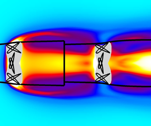
Figure 5. Time-averaged values of pressure coefficient $C_P$ (a) and non-dimensional vorticity $\varOmega c / U_{\infty }$ (anticlockwise positive, b) for Case 1. The grey region in each plot indicates the cross-section of the area swept by the foil, black lines show the time-average streamtube that defines the control volume used for analysis.

Figure 6. Time-averaged values of non-dimensional steady kinetic energy (KE) $= 0.5(U^2+V^2)/U_{\infty }^2$ (a) and unsteady KE $=0.5(\overline {u'u'}+\overline {v'v'})/U_{\infty }^2$ (b) for Case 1.

Figure 7. Instantaneous non-dimensional vorticity $\omega c / U_{\infty }$ (anticlockwise positive), $t/T = 0.125$, for Case 1. Black lines show the time-average streamtube.

Each of the terms in (3.1)–(3.6) and (3.10) is now integrated on the control surface shown in figure 5, to determine their respective contributions to the force and power output from the flapping foil turbine. The upstream and downstream boundaries (inlet and exit of the streamtube) are placed at $x/c=-19.5$ and $x/c=39.5$ respectively, just inside the boundaries of the computational domain. In the modified Betz analysis the effect of oscillating forces and velocities through the turbine plane in (3.10) is calculated by spatially averaging the velocity components across the turbine plane at each time step to obtain $u_{T_i}$, then subtracting off the time-averaged values $U_{T_i}$ to obtain the fluctuating velocities $u'_{T_i}$, and multiplying by the instantaneous fluctuating force components $f'_i$ derived from (2.6); $\dot {W}_{LT}$ is then determined by subtracting the product of force and velocity from the overall power and thus accounts for viscous dissipation of mechanical energy, as well as any effects that cannot be directly measured such as that introduced by the spatial averaging process where the velocity components across the turbine plane are non-uniform.

The efficacy of the control volume approach developed in § 3.1 is tested here, with the results shown in table 1. The power developed by the flapping foil may be calculated directly from instantaneous forces and moments on the foil surface and the translational and rotational velocities as $\dot {W} = f_y \dot {y} + M \dot {\theta }$, and the efficiency obtained from (3.8). Equation (3.11) is then used to calculate the efficiency via the CV approach for comparison, using the calculated coefficient values in table 2. The time-averaged drag coefficient on the turbine is also compared.

Table 1. Comparison between time-averaged power coefficient $\bar {C}_P$, time-averaged drag coefficient $\bar {C}_D=F_x/(0.5\rho U_{\infty }^2 c)$ and efficiency $\eta$. Values taken from the literature (Kinsey & Dumas Reference Kinsey and Dumas2008), direct measurement from foil surface and via CV approach from (3.11) (Case 1).

Table 2. Force and power coefficient contributions integrated over the complete streamtube (Case 1). Definitions of the coefficients given in (3.6) and (3.10).

We see that there is very good agreement between all three sets of values (note that Kinsey & Dumas (Reference Kinsey and Dumas2008) reported values of $\eta =0.337$ and $\bar {C}_P=0.86$, and the value of $\bar {C}_P=0.863$ given in table 1 is inferred from the value of $\eta$ and the known value of the trailing edge vertical swept distance $d$). The slight discrepancy in the direct power and efficiency values compared to the literature is considered acceptable given the differing numerical approaches used to solve the flow. The close similarity between the direct and CV-based values of force, power and the actual efficiency of the turbine from (3.11) gives a high degree of confidence in the methodology, and its ability to then predict the maximum potential efficiency from (3.16).

Figure 8 shows the contribution of terms in (3.6), as a function of distance along the streamtube sides (i.e. excluding the contributions from the CV upstream and downstream boundaries). Here, the upstream control volume boundary is kept fixed at $x/c=-19.5$, and the contributions integrated from that point to a variable point represented by the $x/c$ coordinate, thus these are cumulative contributions from the upstream boundary to the point plotted. We see weak force contributions from viscous effects and pressure along the streamtube sides, but a strong diffusion of unsteady momentum from the Reynolds stress (represented by the $C_{FR}$ term) into the streamtube between 0 and 4 chords downstream of the foil pivot. See figure 7 for an illustration of this occurring in the instantaneous flow field. Momentum is removed between 4 and 7 chords, then increases and decreases again several times further downstream, corresponding to the locations in figure 5 where strong vorticity is crossing the streamtube sides.

Figure 8. Force and power coefficient contributions on the sides of the streamtube, integrated from the control volume inlet to the value of $x/c$ indicated (Case 1).

Examining the power contributions, $C_{WPA}$ on the streamtube sides is exactly zero as expected due to the time-averaged flow field being aligned to the streamtube, so is not plotted here. There is a relatively weak negative contribution in $C_{WPF}$ (power reduced by correlation of fluctuating pressure and velocity), and as expected the work from viscous forces on the streamtube sides is also very small. There is a large contribution from $C_{WA}$ representing convection of unsteady kinetic energy ($\overline {u'_i u'_i}U_j$), work done by Reynolds stresses ($2 U_i \overline {u'_i u'_j}$) and transport of unsteady kinetic energy by fluctuating velocities ($\overline {u'_i u'_i u'_j}$), with a similar spatial distribution as $C_{FR}$. The strongest contributor to $C_{\beta }$ in this case is the viscous dissipation of mechanical energy represented by a relatively large negative value of $C_{WC}$.

Examining the values of $C_{\alpha }$ and $C_{\beta }$ from table 2 we see that for this set of flapping kinematic parameters, there are effects ignored in the standard Betz analysis that make a strong contribution to the force and power output. This is particularly true of the force due to diffusion of unsteady momentum across the streamtube sides $(C_{FR}=0.1576)$ which is approximately a quarter of that due to momentum in and out of the streamtube through the inlet and exit $(C_{FM}=0.5945)$. There is also a strong contribution to force due to non-free-stream pressure on the downstream exit of the streamtube. In the Betz analysis the pressure far downstream is assumed to be equal to free stream; however, here we see that even 40 chords downstream, the pressure is non-uniform across the wake, and low pressure regions are correlated with the mean path of vorticity shed from the flapping foil as shown in figure 5, indicating that these vortices remain coherent far downstream. Overall the additional terms make almost as much contribution to force as does the momentum flux ($C_{\alpha } / C_{FM} = 0.77$), with various contributions to the power almost cancelling in this case, but regardless large enough to indicate that they should not be ignored.

3.4. Interpretation of single foil results

Figure 9 shows the $C_{\alpha }$ and $C_{\beta }$ results obtained above, overlaid on the potential maximum efficiency contours plotted as in figure 2, but now with the non-zero value of $C_{\gamma }$ available to use in the calculation of (3.16). Case 1 falls just short of the region where $\eta _{max}$ is theoretically greater than the Betz limit of $16/27$, yet is well short of this value in the actual efficiency achieved. Also using measured values of inlet area $A_1$ and turbine plane area $A_T$ and mass conservation $U_T / U_{\infty } = A_1 / A_T$, gives $U_T / U_{\infty } = 0.7306$ for Case 1, somewhat higher than the optimum Betz value of $2/3$. To understand this discrepancy between potential and actual performance we must first return to the definition of efficiency in (3.8) and (3.12).

Figure 9. Contours of $\eta _{max}$ vs $C_{\alpha }$ and $C_{\beta }$ from (3.15) and (3.16), with $C_{\gamma }=0.35$. Values from singe foil Case 1 annotated.

Equation (3.8) (or in coefficient form, (3.11)) states that the efficiency is determined by the balance of kinetic energy fluxes entering and leaving the streamtube used as the control volume, along with effects from viscous dissipation and fluctuating forces and velocities through the turbine plane. If we first fix the denominator (constant mean force on the turbine), to increase efficiency we must increase the net power which may be achieved by a positive $C_{\beta }$ in (3.12). If instead we allow the denominator to change, additional force on the turbine ($C_{\alpha }$ increasing) acts to slow the turbine plane velocity $U_T$ as seen in figure 3, and additional energy must then be added to the streamtube to overcome this, leading to the observed shape of the shaded region in figures 2 and 9.

Why then does Case 1 come close to the shaded region in figure 9, thus indicating a very high potential performance, yet not achieve an actual efficiency anywhere near the Betz limit? The answer is that the analysis of the single foil in § 3.1 does not take into consideration where in the streamtube that extra energy is entering, just that it is entering somewhere. Figure 8 shows very clearly that energy enters several to many chords downstream of the turbine plane, where it is not available to pass through and be extracted by the turbine. Figure 6 shows that while significant kinetic energy is generated by the unsteady behaviour of the vortices shed from the foil, this manifests itself in the wake of the foil within the time-averaged stream tube, and little additional kinetic energy is entrained into the streamtube as a result. So the maximum theoretical efficiency might exceed the Betz limit, but in practice that efficiency will never be achieved as the extra energy is not used and escapes downstream.

The entry point of this additional energy is governed by the nature of the flapping foil and the flow dynamics that is induced, and will necessarily be downstream of the turbine plane as the generated leading and trailing edge vortices are convected by the mean flow. Thus a single flapping foil turbine can still be said to be limited by the Betz efficiency in practice. This analysis raises the prospect, however, that a second foil placed in tandem several chords downstream of the first, may experience a meaningful benefit of the additional energy induced by the unsteady action of the upstream foil. In what follows, the analysis is further developed to consider just such a tandem foil geometry.

4.1. Modification of the Newman analysis

Newman (Reference Newman1986) analysed the performance of an array of an arbitrary number of equally sized turbines placed one behind the other, with the same assumptions as in the standard Betz analysis (steady flow, atmospheric pressure on all streamtube boundaries, no viscous effects, purely axial flow). This work used the Bernoulli equation applied along streamlines between and around the turbines to find a maximum achievable efficiency for two tandem turbines of $0.64$, and $0.66$ for an infinite number of turbines. We use the terminology of tandem-turbine Betz limit and Newman limit interchangeably, believing the former is the more recognisable form.

Here we perform a similar analysis using control volumes, in a manner more amenable to including the additional momentum and energy transport terms that result from the unsteady behaviour of the flapping foils. This is done for two tandem foils, as shown in figure 10, but may be extended to an arbitrary number of foils in a relatively straightforward manner (that is to say setting up the analysis is straightforward, but as will become apparent the complexity of the solutions rapidly increases once more than one foil is considered). Once again the analysis makes no assumption of dimensionality of the control volumes.

Figure 10. Time-averaged streamtubes (solid lines) as the control surfaces for tandem flapping foil turbines $T_1$ and $T_2$ (nominal planes with areas $A_1$ and $A_2$ represented by dash-dot lines, see figure 1 for the relationship between these planes and the physical foils). Streamlines are shown as dotted lines. Despite the optical illusion, turbine areas $A_1$ and $A_2$ are equal in this figure.

In figure 10 the same approach is used as for the single foil case, where the leading turbine $T_1$ is enclosed in a control surface $CS_1$ which starts far upstream, follows the time-average streamlines that pass through the limits of the swept area of the turbine, but now terminates at the midpoint $M$ between $T_1$ and the trailing turbine $T_2$. This trailing turbine is similarly enclosed in control surface $CS_2$ which starts at the midpoint $M$, follows the streamlines passing through the limits of the swept area of $T_2$, and ends far downstream. Control surfaces which entirely enclose the foils, rather than abutting them or crossing them (as in Newman Reference Newman1986) are deliberately chosen here due to the need to perform time averaging of computational fluid dynamics (CFD) solutions. This approach avoids the question of how to appropriately calculate the time-average value of any flow quantity, at a point in the flow through which the foil passes at some times during the flapping cycle, i.e. where there is fluid–solid intermittency. The velocity at midpoint $M$ is assumed to be constant across the exit of $CS_1$, as in Newman (Reference Newman1986), with any vertical component negligible in comparison to the horizontal component.

The efficiency of the entire system is given by (3.8), with the power output now split between the two foils

(4.1)\begin{equation} \eta = \frac{\overline{\dot{W}}}{\frac{1}{2}\rho U_{\infty}^3 A_T} = \frac{\overline{\dot{W}}_1+\overline{\dot{W}}_2}{\frac{1}{2}\rho U_{\infty}^3 A_T},\end{equation}

with both turbines assumed to have the same swept area $A_T$, without loss of generality. In situations where the areas differed, the largest would be used in the calculation of the overall efficiency of the system.

Similarly the power output of each individual foil may be defined by the forces on and velocities through the turbine plane, along with any losses of mechanical energy across it as in (3.7). The time-average horizontal velocities through each turbine $U_{T1}$ and $U_{T2}$ are solved for and then substituted into the expression for efficiency to give

(4.2)\begin{align} \eta &= \frac{\overline{\dot{W}}_1}{\frac{1}{2}\rho U_{\infty}^3 A_T} + \frac{\overline{\dot{W}}_2}{\frac{1}{2}\rho U_{\infty}^3 A_T} \nonumber\\ &= \frac{1}{\frac{1}{2}\dot{m}_1U_{\infty}^3}\frac{\overline{\dot{W}}_1}{{F_x}_1}(\overline{\dot{W}}_1 - {\overline{(f'_i u'_{T_i})}}_1+ \overline{\dot{W}}_{LT1}) \nonumber\\ & \quad + \frac{1}{\frac{1}{2}\dot{m}_2U_{\infty}^3}\frac{\overline{\dot{W}}_2}{{F_x}_2} (\overline{\dot{W}}_2 - {\overline{(f'_i u'_{T_i})}}_2+ \overline{\dot{W}}_{LT2}) \nonumber\\ &= \frac{(C_{WKE1}+C_{\beta1})(C_{WKE1}+C_{\beta1}+C_{\gamma1})}{C_{FM1}+C_{\alpha1}} \nonumber\\ & \quad + \frac{(C_{WKE2}+C_{\beta2})(C_{WKE2}+C_{\beta2}+C_{\gamma2})}{C_{FM2}+C_{\alpha2}}, \end{align}

where $\dot {m}_1 = \rho U_{T1} A_T$ and $\dot {m}_2 = \rho U_{T2} A_T$ are the mass flow rates through the upstream and downstream turbines respectively. We now define force and power coefficient terms as per (3.4)–(3.6) for each of the control surfaces, but with slightly differing non-dimensionalising factors as in table 3.

Table 3. Non-dimensionalising factors for force and power coefficients for upstream and downstream turbines.

Integrating over the control surfaces as for the single foil case results in

(4.3)\begin{align} \eta &= \frac{\left(1-a^2+C_{\beta1}\right)\left(1-a^2+C_{\beta1}+C_{\gamma1}\right)}{2(1-a)+C_{\alpha1}} \nonumber\\ & \quad+ \frac{\left(a^2-b^2+C_{\beta2}\right)\left(a^2-b^2+C_{\beta2}+C_{\gamma2}\right)}{2(a-b)+C_{\alpha2}}, \end{align}

where now velocity ratios $a = U_M / U_{\infty }$ and $b = U_{E} / U_{\infty }$ are defined, and $A_{M1}$ and $A_{M2}$ are the areas of the exit of $CS_1$ and inlet of $CS_2$ respectively. Following the same procedure as for the single foil case, one may in principle find an expression for the maximum possible efficiency $\eta _{max}$ by differentiating $\eta$ with respect to $a$ and $b$, setting both results to zero to obtain two equations for the two unknowns $a_{opt}$ and $b_{opt}$, and substituting these back into (4.3). This is done first as a check with $C_{\alpha 1} = C_{\alpha 2} = C_{\beta 1} = C_{\beta 2} = C_{\gamma 1} = C_{\gamma 2} = 0$, where the resulting equations are straightforward to solve (although there are four solutions, only one of which is physical), resulting in $a_{opt}=U_M / U_{\infty } = 3/5$, $b_{opt}=U_{E} / U_{\infty } =1/5$, and $\eta _{max}=16/25 = 0.64$. This is precisely the result obtained by Newman (Reference Newman1986) for a two turbine system, giving confidence in the methodology used here.

The equations may in principle be solved exactly as for a single foil, although when all the additional force and power coefficients are non-zero the process of maximisation becomes too complex to solve in symbolic form; thus for any given values of the coefficients, $a_{opt}$, $b_{opt}$ and $\eta _{max}$ are obtained numerically. For this more general case, there are multiple solutions for each set of coefficient values, and these are reduced to the single physical solution by application of the constraints $0 < a_{opt} < 1$, $0 < b_{opt} < 1$, $b_{opt} < a_{opt}$ (the flow velocity must be reduced through each turbine, and cannot be reversed in direction), $\partial ^2\eta / \partial a^2 < 0$ and $\partial ^2\eta / \partial b^2 < 0$ (the final two being imposed to ensure a genuine maximum in the efficiency rather than an inflection point).

With six independent variables instead of three, the dependence of efficiency on the force and power coefficients is difficult to show graphically. Four special cases are illustrated in figure 11. In figures 11(a) and 11(b) the constraints ensuring non-imaginary solutions are solved exactly and are indicated in equation form on the figure, whereas in figures 11(c) and 11(d) the constraints are determined numerically and do not have a closed-form solution. As for the single foil case, there are clearly sizeable regions of this space where the tandem-turbine Betz limit is theoretically exceeded, and it is necessary to determine whether the coefficient values required to push the overall efficiency up to or beyond that limit can actually be achieved. In particular, the entry of momentum and energy through the sides of the control volume ahead of the downstream turbine, induced by the unsteady action of the upstream turbine, will be examined in detail. The separation distance between the upstream and downstream turbines also clearly becomes an important parameter, discussed further below.

Figure 11. Region of $C_{\alpha 1}$, $C_{\alpha 2}$, $C_{\beta 1}$, $C_{\beta 2}$ space (shaded) for which $16/25 < \eta _{max} < 1$. (a) $C_{\alpha 2} = C_{\beta 2} = 0$; (b) $C_{\alpha 1} = C_{\beta 1} = 0$; (c) $C_{\alpha 1} = C_{\alpha 2} = 0$; (d) $C_{\alpha 1} = C_{\alpha 2} = 0.25$. $C_{\gamma 1} = C_{\gamma 2} = 0$ in each panel.

4.2. Evaluation of non-idealised momentum and energy terms

Once again 2-D tandem foil flapping parameter combinations were chosen inspired by cases from the literature, to examine the relative size and impact of each of the terms comprising $C_{\alpha 1}$, $C_{\alpha 2}$, $C_{\beta 1}$, $C_{\beta 2}$, $C_{\gamma 1}$ and $C_{\gamma 2}$. Case 2 was based upon Kinsey & Dumas (Reference Kinsey and Dumas2012b) representing the most efficient case from that study (they reported a maximum efficiency of $\eta =0.641$, right at the tandem foil Betz limit). Since force and power time histories of the upstream and downstream foils were not available for this case in Kinsey & Dumas (Reference Kinsey and Dumas2012b), two more cases (here referred to as 3 and 4) for which they were available were considered to act as validation of the numerical solver.

In Case 2 the upstream foil is a NACA0015 aerofoil oscillating in heave $y_1(t)=hc\sin (\omega t)$ and pitch $\theta _1(t)=\theta _0\sin (\omega t + \phi )$, pitching about the $1/3$ chord point with heave amplitude $h=1.0$ chords, pitch amplitude $\theta _0=75.0^{\circ }$, pitch leading heave with phase $\phi =90^{\circ }$, non-dimensional frequency $f^*=fc/U_{\infty }=0.14$, at Reynolds number ${\textit {Re}}=5.0\times 10^5$. The second foil is placed downstream from the first with a distance of $5.4$ chords separating their respective pivot points and with identical geometry and motion parameters, except that the downstream foil oscillates out of phase relative to the upstream foil, i.e. $y_2(t)=hc\sin (\omega t + \phi _{1-2})$ and pitch $\theta _1(t)=\theta _0\sin (\omega t + \phi + \phi _{1-2})$ with $\phi _{1-2} = 180^{\circ }$. Kinsey & Dumas (Reference Kinsey and Dumas2012b) simulated a range of separation distances and inter-foil phases with these values producing the highest efficiency found for the chosen individual foil kinematics at this Reynolds number. They argued that critical to the high efficiency achieved was a strong interaction between the downstream foil and the shed vortices of the upstream foil, and those vortices entraining additional momentum and energy to increase the dynamic pressure of the flow that the downstream foil would otherwise be exposed to.

Case 3 is identical to Case 2, except for a reduced pitch amplitude ($\theta _0=70.0^{\circ }$). Case 4 is identical to Case 3 except for an increased flapping frequency ($\,f^*=0.18$).

The solver employed for the single foil cases is unsuitable here due to the much higher Reynolds number, so the commercial code ANSYS Fluent 19.2 is used. The computational domain is $72.8c\times 40c$ with domain boundaries at $21.4c$ upstream of the leading foil pivot point and $46c$ downstream of the trailing foil pivot point (plus $5.4c$ separation between the pivot points), and $20c$ in each cross-stream direction. A second-order pressure-based coupled scheme is used to solve the incompressible Navier–Stokes equations, and the $k\text{-}\omega$ SST turbulence model (see Menter Reference Menter1994) is used with turbulent viscosity ratio of 1.0 and turbulence intensity of 0.1 % assumed at the upstream inlet. The overset mesh technique is used, with high resolution body-fitted grids around the foils (200 cells along the foil chord, and first cell spacing of $1.0\times 10^{-6}$ chords, resulting in $y^+<1.0$ at all times) and a multi-block Cartesian background grid (with spacing $\Delta x=\Delta y=0.0125c$ gradually increasing away from the foils and wake region). Total cell count is approximately 750 000 and there are 2000 time steps per flapping cycle. The simulations were run for 18 flapping cycles to ensure periodicity of the solution, with the final 8 cycles used for time averaging.

The Case 2 simulation resulted in a combined efficiency for the upstream and downstream foils of $\eta =0.653$, very close to the $0.641$ predicted by Kinsey & Dumas (Reference Kinsey and Dumas2012b). Case 3 and 4 results were $0.620$ vs $0.614$, and $0.532$ vs $0.521$, respectively. In addition, figure 12 shows the high level of agreement in vertical force generated by the upstream and downstream foils, between the present simulations and the literature on which Cases 3 and 4 are based. While there are some very small discrepancies in the vertical force time histories leading to the differences in the computed efficiencies, most likely due to differences in mesh construction and motion strategy between the present work (overset mesh) and the literature (non-conformal sliding mesh), the quantitative and qualitative levels of agreement are considered high for these three different foil kinematics, indicating that details of vortex shedding and other interactions between the upstream foil wake and the downstream foil have been successfully captured. While unsteady RANS was used here for direct comparison with Kinsey & Dumas (Reference Kinsey and Dumas2012b), at this Reynolds number there are likely to be smaller scale vortical structures overlaid on the larger scales captured by the solver. It was considered that this was unlikely to significantly affect the conclusions to be drawn from this analysis, although a fuller treatment in three dimensions with large eddy simulation is suggested for future work as noted at the end of this section.

Figure 12. Comparison of simulation results (CFD) against Kinsey & Dumas (Reference Kinsey and Dumas2012b). Instantaneous lift coefficient $C_L = F_y / \frac {1}{2}\rho U_{\infty }^2 c$, Case 3 (a) and Case 4 (b), parameters given in § 4.2. $\text {US = upstream foil}$, $\text {DS = downstream foil}$.

Since Case 2 involves turbulent flow simulated using an unsteady RANS turbulence model ($k$-$\omega$ SST), the solver tracks two additional variables in addition to the pressure and velocities, namely turbulent kinetic energy $k$ and specific dissipation rate $\omega$. The only interaction between the turbulence and the momentum equation in the solver is through modification of the viscosity (addition of the so-called turbulent viscosity $\mu _T$ derived from $k$ and $\omega$ in the turbulence model). Thus (2.6) requires no modification other than using $\mu +\mu _T$ in calculation of the shear stress $\tau _{ij}$ instead of $\mu$. At this point it should be noted that the conservation of mechanical energy equation is not explicitly solved by the CFD solver. Rather (2.7) represents the conservation equation that is inherently satisfied by the CFD solutions, and is derived by multiplying (2.6) by instantaneous velocity vector $u_i$ and summing over tensor indices. Since the flow field is modified by the effects of turbulence via the turbulent viscosity, such effects are inherently included in the energy equation, including the additional turbulent dissipation and similarly do not require separate treatment. For completeness though in the following analysis we examine the magnitude of the transport of turbulent kinetic energy for comparison with the other energy transport mechanisms. In the time-averaging time scale of one flapping period, this turbulent kinetic energy can be considered to have steady and fluctuating components

(4.4a,b)\begin{equation} k(t) = K+k', \quad K=\bar{k}=\frac{1}{T}\int_t^{t+T} k(t)\,\textrm{d} t. \end{equation}

Figure 13 shows the time-averaged values of the pressure coefficient and non-dimensional vorticity, with the control surfaces $CS_1$ and $CS_2$ defined as the streamlines based on the time-averaged velocities $U$ and $V$ passing through the maximum extent of the swept area of the upstream and downstream flapping wings, respectively. The exit of $CS_1$ and the inlet of $CS_2$ are both placed at the midpoint between the two nominal turbine planes, in correspondence with the schematic shown in figure 10. As in the single foil Case 1, there is significant pressure variation along the streamtube boundaries, although the pressure field is no longer strongly correlated with the time-averaged vorticity. Comparison of kinetic energy components in figure 14 shows that unsteady KE is a significant proportion of the total entering the inlet of the downstream streamtube and into the turbine plane, confirming predictions made at the end of § 3.4. This is also readily apparent in figure 15, where the downstream foil is observed strongly interacting with the vortex wake shed from the upstream foil. Interestingly both the unsteady KE and steady turbulent $K$ in figure 14 show streams coming from the trailing edge of the upstream foil and entering the sides of the downstream streamtube, just ahead of the downstream foil, supporting the optimality of the chosen separation distance. This behaviour is similar to the laminar case in figure 6, although there the two streams do not diverge as widely and come together much closer to the upstream foil, only about two chords downstream of the nominal turbine plane. This suggests that the ideal separation distance between upstream and downstream foils would be strongly influenced by Reynolds number. It is noted that the turbulent kinetic energy in this case is an order of magnitude smaller than the unsteady kinetic energy, and is also not as strongly transported into the downstream streamtube (lacking the strong central ‘jet’ of unsteady KE shown behind the upstream foil). Thus the effect of the turbulent flow in Case 2 is to alter the vortex shedding and wake of the two turbines in comparison to the laminar single foil cases, rather than contributing directly to the downstream turbine energy budget.

Figure 13. Time-averaged values of pressure coefficient $C_P$ (a) and non-dimensional vorticity $\varOmega c / U_{\infty }$ (anticlockwise positive, b) for Case 2. The grey regions in each panel indicate the cross-section of the areas swept by the foils, black lines show the time-average streamtubes.

Figure 14. Time-averaged values of non-dimensional steady KE $=0.5(U^2+V^2)/U_{\infty }^2$ (a), unsteady KE $=0.5(\overline {u'u'}+\overline {v'v'})/U_{\infty }^2$ (b) and turbulent $K/U_{\infty }^2$ (c) for Case 2. Note colour scale differences between panels, emphasising the relative sizes of the energy components.

Figure 15. Instantaneous non-dimensional vorticity $\omega c / U_{\infty }$ (anticlockwise positive), $t/T = 0.035$, for Case 2. Black lines show the time-average streamtubes.

Now we must look closely at the breakdown of the momentum and energy components entering the streamtubes. Noting the discussion at the end of § 3.4, it makes little sense to quantify the $C_{\alpha }$ and $C_{\beta }$ values for each control surface in its entirety, but rather to look only at components which flow into the control surface ahead of the turbine, and hence are available for use by that turbine and will have a material effect on the performance. Thus the exit for each streamtube is taken to be at the maximum horizontal extent of the flapping motion of the foil trailing edge (just aft of the nominal turbine plane). As was done for the single foil case, we first check the efficacy of the control volume approach in measuring the actual performance of the tandem foil turbine system, before using it to predict the maximum potential performance. Table 4 shows very good agreement between the overall and individual foil efficiencies comparing values from Kinsey & Dumas (Reference Kinsey and Dumas2012b) and the present calculation, when measuring forces and moments directly on the foil surfaces. Importantly the control volume analysis also yields the same level of agreement in the overall system efficiency and in the breakdown between the upstream and downstream foils, giving a high degree of confidence in the ability of the method to predict the maximum potential efficiency of the system.

Table 4. Comparison of upstream ($\eta _1$), downstream ($\eta _2$) and total efficiency ($\eta$). Values taken from the literature (Kinsey & Dumas Reference Kinsey and Dumas2012b), direct measurement from foil surface and via CV approach (Case 2).

The various coefficients used in the calculation of the CV-based efficiencies in table 4 are provided in table 5. Examining the values of $C_{\alpha 1}$, $C_{\beta 1}$, $C_{\alpha 2}$, $C_{\beta 2}$, $C_{\gamma 1}$ and $C_{\gamma 2}$ shows that in this tandem foil Case 2, as for the single foil Case 1, there are significant effects not considered in the standard Betz analysis. Once again there is a major contribution from non-uniform pressure in terms of the force placed on the control surface seen in $C_{FP}$, and in the flow work $C_{WPA}$. This is true of both upstream and downstream foils. Reynolds stresses seen in $C_{FR}$ also contribute to the forces, through the sides of $CS_1$ and the sides and inlet of $CS_2$ although the contribution is small in comparison to the pressure. Interestingly for this case the transport of unsteady kinetic energy and steady turbulent kinetic energy via the steady flow field, as well as flow work done by the Reynolds stresses, showing up in the $C_{WA}$ terms, produces slightly negative values. Thus the overall effect of unsteady energy transport is removing some energy from that available for both foils, rather than adding it as expected. However, the negative effect from $C_{WA}$ for the downstream foil is only one third the magnitude of the upstream foil value, suggesting that in comparison the downstream foil is benefiting from the unsteady flows of energy from the upstream foil. The viscous dissipation $C_{WC}$ terms are negative (as they must be), but are relatively much less strong than for the single foil case, which is reasonable given the much higher Reynolds number of the tandem foil case. Overall the size of the $C_{\alpha }$ and $C_{\beta }$ terms in comparison to the standard momentum and energy flux terms $C_{FM}$ and $C_{WKE}$, for both upstream and downstream terms, show that they cannot sensibly be ignored.

Table 5. Force and power coefficient contributions from upstream (subscript 1) and downstream (subscript 2) foils (Case 2). Definitions of the coefficients given in (3.6) and (3.10). Note the different non-dimensionalisation of upstream and downstream coefficients as given in table 3.

Referring to (4.3) with the measured values of $C_{\alpha 1}$, $C_{\beta 1}$, $C_{\alpha 2}$, $C_{\beta 2}$, $C_{\gamma 1}$ and $C_{\gamma 2}$ in table 5, we may now calculate the optimum velocity ratios $a = U_M / U_{\infty }$ and $b = U_{E} / U_{\infty }$ and the corresponding maximum efficiency for Case 2. This gives results of $a_{opt}=0.503$, $b_{opt}=0.177$ and $\eta _{max}=0.777$, an efficiency significantly beyond the achieved value of $0.644$, and well outside the variation seen in the three different values in table 4. This result, shown graphically in figure 16, suggests that there is scope for improvement in the already high performance achieved by the tandem foil system, and an efficiency somewhat beyond the tandem-turbine Betz (Newman) limit of $\eta =0.64$, at least for high aspect ratio foils where the flow is predominantly two-dimensional as examined here.

Figure 16. Contours of overall system $\eta _{max}$ from (4.3), values from tandem foil Case 2 annotated. Shaded region indicates $16/25 < \eta _{max} < 1$. Contours equally spaced between the lowest and highest $\eta _{max}$ values indicated in each frame. (a) $C_{\alpha 2}$ and $C_{\beta 2}$ variable, all other values as per table 5. (b) $C_{\beta 1}$ and $C_{\beta 2}$ variable, all other values as per table 5.

As pointed out in § 3.1 the analysis method is applicable to 3-D flows, although the evaluation of the unsteady effects has been conducted here in two dimensions. Kinsey & Dumas (Reference Kinsey and Dumas2012a) examined the performance of a 3-D rectangular planform foil of aspect ratio 7.0 with endplates, at ${\textit {Re}}=5.0 \times 10^5$. Simulations in three dimensions showed excellent agreement with experimental results, with a 15 %–16 % reduction in power generation compared to the same case in two dimensions. Further work (Kinsey & Dumas Reference Kinsey and Dumas2012c) at different aspect ratios with and without endplates resulted in power reductions of 20 %–30 % compared to the equivalent 2-D cases. This was attributed to changes in structure and diminution of leading edge vortices at the foil tips and interaction with the trailing tip vortices. The question arises whether the reduction in performance seen in three dimensions would thus definitively preclude the tandem-turbine Betz limit being exceeded in practice. This will again depend on whether the flow of additional unsteady momentum and energy (i.e. unaccounted for in the standard steady analysis) is into or out of the control volume sides behind the tips of the leading foil. Visualisations of the 3-D wake structure are available in the literature for a single finite aspect ratio foil in propulsive (e.g. Buchholz & Smits Reference Buchholz and Smits2008) and power extracting (e.g. Kim et al. Reference Kim, Strom, Mandre and Breuer2017) regimes, in the form of dye streaklines and vorticity iso-surfaces. However, figures 13–15 show that it is difficult to infer the flow of unsteady kinetic energy from the time-averaged vorticity field, and harder again from the instantaneous vorticity. Therefore 3-D simulations of the turbulent flow around tandem flapping foil turbines with high resolution of the wake structures, time averaged over many flapping cycles to ensure statistically stationary results, are needed to answer this question more fully.