2. Derivation of the momentum equation and the particle--particle drag relation

For completeness, a brief review of the derivation of the momentum equation for a particular particle type is shown as follows, and readers can refer to Garzo, Dufty & Hrenya (Reference Garzo, Dufty and Hrenya2007), Marchisio & Fox (Reference Marchisio and Fox2013) and Zhao & Wang (Reference Zhao and Wang2021) for more details. The single-particle VDF of particle type i is denoted by ${f_i}({\boldsymbol{c}_i},\boldsymbol{r},t)$, and ${f_i}({\boldsymbol{c}_i},\boldsymbol{r},t)\,\textrm{d}{\boldsymbol{c}_i}\,\textrm{d}\boldsymbol{r}$ is equivalent to the probable number of particles in the velocity and position element $\textrm{d}{\boldsymbol{c}_i}\,\textrm{d}\boldsymbol{r}$ at time t. Similarly, the two-particle VDF is represented by $f_{ij}^{(2)}({\boldsymbol{c}_i},{\boldsymbol{r}_i},{\boldsymbol{c}_j},{\boldsymbol{r}_j},t)$, and $f_{ij}^{(2)}({\boldsymbol{c}_i},{\boldsymbol{r}_i},{\boldsymbol{c}_j},{\boldsymbol{r}_j},t)\,\textrm{d}{\boldsymbol{c}_i}\,\textrm{d}{\boldsymbol{r}_i}\,\textrm{d}{\boldsymbol{c}_j}\,\textrm{d}{\boldsymbol{r}_j}$ equals the probable number of the particle pairs in which the two particles are respectively lying in velocity and position elements $\textrm{d}{\boldsymbol{c}_i}\,\textrm{d}{\boldsymbol{r}_i}$ and $\textrm{d}{\boldsymbol{c}_j}\,\textrm{d}{\boldsymbol{r}_j}$. The spatio-temporal evolution of the single-particle VDF is described by the Boltzmann equation

(2.1)\begin{equation}\frac{{\partial {f_i}}}{{\partial t}} + {\boldsymbol{c}_i}\boldsymbol{\cdot }{\nabla _{\boldsymbol{r}}}{f_i} + {\nabla _{{\boldsymbol{c}_i}}}\boldsymbol{\cdot }({\boldsymbol{a}_i}\,{f_i}) = \frac{{{\partial _e}\,{f_i}}}{{\partial t}},\end{equation}

where ${\nabla _{\boldsymbol{r}}}$ and ${\nabla _{{\boldsymbol{c}_i}}} \cdot $ are the gradient with respect to the position $\boldsymbol{r}$ and the divergence with respect to the velocity ${\boldsymbol{c}_i}$, respectively, and ${\boldsymbol{a}_i}$ is the acceleration of a particle of type i due to the external force, such as the gas–particle drag force. The term on the right-hand side represents the rate at which the single-particle VDF is changed by collisions and has the following form:

(2.2)\begin{align}\frac{{{\partial _e}\,{f_i}}}{{\partial t}} = \sum\limits_j {\iint_{\boldsymbol{g}\boldsymbol{\cdot }\boldsymbol{k} > 0} {\left[ {\frac{1}{{e_{ij}^2}}f_{ij}^{(2)}(\boldsymbol{c}_i^b,\boldsymbol{r},\boldsymbol{c}_j^b,\boldsymbol{r} - {d_{ij}}\boldsymbol{k},t) - f_{ij}^{(2)}({\boldsymbol{c}_i},\boldsymbol{r},{\boldsymbol{c}_j},\boldsymbol{r} + {d_{ij}}\boldsymbol{k},t)} \right]} d_{ij}^2(\boldsymbol{g}\boldsymbol{\cdot }\boldsymbol{k})\,\textrm{d}\boldsymbol{k}\,\textrm{d}{\boldsymbol{c}_j}} .\end{align}

Here, ${e_{ij}}$ is the coefficient of restitution, ${d_{ij}}$ is the arithmetic mean diameter, $\boldsymbol{k}$ is the unit vector directed from the centre of a particle of type i to the centre of a particle of type $j$ and $\boldsymbol{g} = {\boldsymbol{c}_i} - {\boldsymbol{c}_j}$. The superscript b denotes the property before the inverse collision, and the prime will be used to indicate the property after the direct collision. The inverse collision is defined as collisions after which the pre-collision velocities $(\boldsymbol{c}_i^b,\boldsymbol{c}_j^b)$ are changed into $({\boldsymbol{c}_i},{\boldsymbol{c}_j})$, and the direct collision is defined as collisions after which the pre-collision velocities $({\boldsymbol{c}_i},{\boldsymbol{c}_j})$ are changed into $({\boldsymbol{c^{\prime}}_i},{\boldsymbol{c^{\prime}}_j})$.

Let ${\psi _i}$ be any particle property. In general, ${\psi _i}$ is a function of ${\boldsymbol{c}_i}$ and invariable with $\boldsymbol{r}$ and t. The mean value of ${\psi _i}$, i.e. the hydrodynamic property of particle type i, is defined by

(2.3)\begin{equation}{n_i}\langle {\psi _i}\rangle = \int {{\psi _i}\,{f_i}\,\textrm{d}{\boldsymbol{c}_i}} ,\end{equation}

where ${n_i}$ is the particle number density. Multiplying ${\psi _i}$ and integrating over ${\boldsymbol{c}_i}$ on both sides of (2.1) yields the transport equation of particle type $i$

(2.4)\begin{equation}\frac{{\partial {n_i}\langle {\psi _i}\rangle }}{{\partial t}} + {\nabla _{\boldsymbol{r}}}\boldsymbol{\cdot }({n_i}\langle {\psi _i}{\boldsymbol{c}_i}\rangle ) - {n_i}\langle {\boldsymbol{a}_i}\boldsymbol{\cdot }{\nabla _{{\boldsymbol{c}_i}}}{\psi _i}\rangle = {\varPsi _i}({\psi _i}).\end{equation}

Using Taylor expansion and neglecting the second-order and higher-order terms, the collision source term ${\varPsi _i}$ can be decomposed into a collision source term ${\varPhi _i}$ and a collision flux term ${\boldsymbol{\varOmega }_i}$ as follows:

(2.5)\begin{equation}{\varPsi _i}({\psi _i}) = {\varPhi _i}({\psi _i}) - {\nabla _{\boldsymbol{r}}}\boldsymbol{\cdot }{\boldsymbol{\varOmega }_i}({\psi _i}),\end{equation}

where

(2.6)\begin{gather}{\varPhi _i}({\psi _i}) = \sum\limits_j {d_{ij}^2} \iint\!\!\!\int_{\boldsymbol{g}\boldsymbol{\cdot }\boldsymbol{k} > 0} {({{\psi ^{\prime}}_i} - {\psi _i}){\chi _{ij}}} \left( {{f_i}\,{f_j} - \frac{{{d_{ij}}}}{2}\boldsymbol{k}\boldsymbol{\cdot }{f_i}\,{f_j}{\nabla_{\boldsymbol{r}}}\ln \frac{{{f_i}}}{{{f_j}}}} \right)(\boldsymbol{g}\boldsymbol{\cdot }\boldsymbol{k})\,\textrm{d}\boldsymbol{k}\,\textrm{d}{\boldsymbol{c}_j}\,\textrm{d}{\boldsymbol{c}_i},\end{gather}

(2.7)\begin{gather}{\boldsymbol{\varOmega }_i}({\psi _i}) = \sum\limits_j {\frac{{d_{ij}^3}}{2}} \iint\!\!\!\int_{\boldsymbol{g}\boldsymbol{\cdot }\boldsymbol{k} > 0} {({{\psi ^{\prime}}_i} - {\psi _i}){\chi _{ij}}} \left( { - {f_i}\,{f_j} + \frac{{{d_{ij}}}}{2}\boldsymbol{k}\boldsymbol{\cdot }{f_i}\,{f_j}{\nabla_{\boldsymbol{r}}}\ln \frac{{{f_i}}}{{{f_j}}}} \right)\boldsymbol{k}(\boldsymbol{g}\boldsymbol{\cdot }\boldsymbol{k})\,\textrm{d}\boldsymbol{k}\,\textrm{d}{\boldsymbol{c}_j}\,\textrm{d}{\boldsymbol{c}_i}.\end{gather}

In the above equations, the correlation of the pre-collision velocities is neglected, i.e. the assumption of molecular chaos, and therefore the two-particle VDF can be written as the product of the two single-particle VDFs with the pair correlation function ${\chi _{ij}}$. For inertial particles, the assumption of molecular chaos is valid when the total solid volume fraction is very small $(\phi \ll 0.1)$. The reason for this is twofold. First, the collision interval is long enough so that post-collision velocities can relax completely. Second, the particle motion is less restricted, leading to a low probability of repeated collisions. Both of these two aspects weaken the correlation between pre-collision velocities. However, for dense systems, the assumption of molecular chaos may be invalid (Chapman & Cowling Reference Chapman and Cowling1970). When ${\psi _i} = {m_i}{\boldsymbol{c}_i}$ where ${m_i}$ is the particle mass, the momentum equation for particle type i is obtained from (2.4) and (2.5) and reads

(2.8)\begin{equation}\frac{{\partial {\phi _i}{\rho _i}{\boldsymbol{u}_i}}}{{\partial t}} + {\nabla _{\boldsymbol{r}}}\boldsymbol{\cdot }({\phi _i}{\rho _i}{\boldsymbol{u}_i}{\boldsymbol{u}_i}) ={-} {\nabla _{\boldsymbol{r}}}\boldsymbol{\cdot }{\boldsymbol{\mathsf{p}}_i} + {\phi _i}{\rho _i}\langle {\boldsymbol{a}_i}\rangle + {\boldsymbol{\varPhi }_i}({m_i}{\boldsymbol{c}_i}).\end{equation}

Here, ${\boldsymbol{u}_i} = \langle {\boldsymbol{c}_i}\rangle $, and ${\phi _i}{\rho _i} = {n_i}{m_i}$, where ${\phi _i}$ and ${\rho _i}$ are respectively the particle volume fraction and the particle mass density. The stress tensor ${\boldsymbol{\mathsf{p}}_i} = {\phi _i}{\rho _i}\langle {\boldsymbol{C}_i}{\boldsymbol{C}_i}\rangle + {\boldsymbol{\varOmega }_i}({m_i}{\boldsymbol{c}_i})$ in which the peculiar velocity ${\boldsymbol{C}_i} = {\boldsymbol{c}_i} - {\boldsymbol{u}_i}$. ${\boldsymbol{\varPhi }_i}({m_i}{\boldsymbol{c}_i})$ is the particle–particle drag force experienced by particle type i per unit volume and is the focus of the present study.

In a collision, the relation between the pre-collision velocity ${\boldsymbol{c}_i}$ and post-collision velocity ${\boldsymbol{c^{\prime}}_i}$ is

(2.9)\begin{equation}{\boldsymbol{c^{\prime}}_i} = {\boldsymbol{c}_i} - \frac{{{m_j}}}{{{m_i} + {m_j}}}(1 + {e_{ij}})(\boldsymbol{g}\boldsymbol{\cdot }\boldsymbol{k})\boldsymbol{k}.\end{equation}

The present study considers the particle–particle drag force at first approximation, so the gradient terms in (2.6) and (2.7) are neglected. Substituting equation (2.9) into the equation of ${\boldsymbol{\varPhi }_i}({m_i}{\boldsymbol{c}_i})$, the integral form of the particle–particle drag force is finally given by

(2.10)\begin{equation}{\boldsymbol{\varPhi }_i}({m_i}{\boldsymbol{c}_i}) ={-} \sum\limits_j {d_{ij}^2} \frac{{{m_i}{m_j}}}{{{m_i} + {m_j}}}(1 + {e_{ij}})\iint\!\!\!\int_{\boldsymbol{g}\boldsymbol{\cdot }\boldsymbol{k} > 0} {{\chi _{ij}}{f_i}\,{f_j}{{(\boldsymbol{g}\boldsymbol{\cdot }\boldsymbol{k})}^2}\boldsymbol{k}\,\textrm{d}\boldsymbol{k}\,\textrm{d}{\boldsymbol{c}_j}\,\textrm{d}{\boldsymbol{c}_i}} .\end{equation}

It should be noted that, due to symmetry, ${\boldsymbol{\varPhi }_i}$ is zero when $i = j$, which means that only collisions between different particle types contribute to the particle–particle drag force. At the first approximation, the single-particle VDF is Maxwellian and reads

(2.11)\begin{equation}{f_i} = \frac{{{n_i}}}{{{{(2{\rm \pi} {T_i})}^{3/2}}}}\,{\textrm{e}^{ - {{({\boldsymbol{c}_i} - {\boldsymbol{u}_i})}^2}\,/(2T_i)}},\end{equation}

where ${T_i}$ is the granular temperature and defined by

(2.12)\begin{equation}{T_i} = \frac{{\langle C_i^2\rangle }}{3}.\end{equation}

Note that the equipartition of the kinetic energy of the peculiar motion indicates ${m_i}{T_i} = {m_j}{T_j}$. Zhao & Wang (Reference Zhao and Wang2021) rigorously derived the particle–particle drag relation from (2.10) and (2.11) without any mathematical approximations, and it is given as

(2.13)\begin{align} {\boldsymbol{\unicode{x1D4BB}}_{\!ij}} & ={-} 2{\rm \pi} d_{ij}^2\dfrac{{{m_i}{m_j}}}{{{m_i} + {m_j}}}(1 + {e_{ij}}){n_i}{n_j}({T_i} + {T_j}){\chi _{ij}}\left[ {\dfrac{1}{{\sqrt {\rm \pi} }}\left( {\dfrac{1}{2} + \dfrac{1}{{4{{\langle {g^\ast }\rangle }^2}}}} \right)\,{\textrm{e}^{ - {{\langle {g^\ast }\rangle }^2}}}} \right.\nonumber\\ & \left. \quad + \left( {\dfrac{{\langle {g^\ast }\rangle }}{2} + \dfrac{1}{{2\langle {g^\ast }\rangle }} - \dfrac{1}{{8{{\langle {g^\ast }\rangle }^3}}}} \right)erf(\langle {g^\ast }\rangle ) \right]\langle {\boldsymbol{g}^\ast }\rangle,\end{align}

in which ${\boldsymbol{g}^\ast } = \boldsymbol{g}/\sqrt {2({T_i} + {T_j})}$ and the error function is defined by $erf(\langle {g^\ast }\rangle ) = (2/\sqrt {\rm \pi} )\int_0^{\langle {g^\ast }\rangle } {{\textrm{e}^{ - {y^2}}}\,\textrm{d}y}$. Notice that the summation notation is dropped in (2.13) since bidisperse mixtures are considered in this study, and $\boldsymbol{\unicode{x1D4BB}}_{\!ij}$ represents the particle–particle drag force on the particle type i exerted by j per unit volume. For the latter analysis, the number of collisions per time per unit volume between particle types i and j is denoted by ${N_{ij}}$, and ${N_{ij}}/{n_i}$, named the collision frequency, is the average number of collisions experienced by a particle of type i with particle type j. The relation of ${N_{ij}}/{n_i}$ proposed by Zhao & Wang (Reference Zhao and Wang2020) is

(2.14)\begin{equation}\frac{{{N_{ij}}}}{{{n_i}}} = \sqrt {2{\rm \pi} } d_{ij}^2{n_j}\sqrt {{T_i} + {T_j}} {\chi _{ij}}\left[ {{\textrm{e}^{ - {{\langle {g^\ast }\rangle }^2}}} + \sqrt {\rm \pi} \left( {{g^\ast } + \frac{1}{{2\langle {g^\ast }\rangle }}} \right)erf(\langle {g^\ast }\rangle )} \right].\end{equation}

When the particle distribution is homogeneous and isotropic, the pair correlation function only depends on the radial distance and degenerates into the radial distribution function. For the contact value of the radial distribution function, Lebowitz (Reference Lebowitz1964) proposed the following expression for a mixture of hard spheres:

(2.15)\begin{equation}{\chi _{ij}} = \frac{1}{{1 - \phi }} + \frac{{3{d_i}{d_j}}}{{{{(1 - \phi )}^2}({d_i} + {d_j})}}\left( {\frac{{{\phi_i}}}{{{d_i}}} + \frac{{{\phi_j}}}{{{d_j}}}} \right),\end{equation}

where the total solid volume fraction $\phi = {\phi _i} + {\phi _j}$. Simulation results show that, in the current parameter range, ${\chi _{ij}}$ is invariant with respect to the Reynolds number, and the prediction error of (2.15) is less than $5 \%$, indicating that the microstructure of the suspensions is close to binary hard-sphere fluids. Therefore, (2.15) is employed in the calculations of the particle–particle drag force and the collision frequency.

3. Simulation method

The second-order accurate immersed boundary-lattice Boltzmann method (IB-LBM) developed by Zhou & Fan (Reference Zhou and Fan2014) is employed to solve the gas flow, and the particle motion is tracked by the DEM. The particle collision is simulated by the soft-sphere model and resolved by 8 LBM time steps, each containing 15 DEM time steps. The reader can refer to the document of MFIX (Garg et al. Reference Garg, Galvin, Li and Pannala2012) for more details. The accuracy of these methods is proved by simulating flow past arrays of rotating spheres (Zhou & Fan Reference Zhou and Fan2015a,Reference Zhou and Fanb) and gas–particle suspensions (Duan et al. Reference Duan, Zhao, Chen and Zhou2020; Zhao, Chen & Zhou Reference Zhao, Chen and Zhou2021). When the gap size between a pair of particles becomes comparable to the grid size, the flow in the gap is not fully resolved, and consequently the lubrication force cannot be correctly computed. In this situation, a theoretical formula (Guazzelli & Morris Reference Guazzelli and Morris2012) is adopted to compensate for the unresolved part of the lubrication force and is given by

(3.1)\begin{equation}\boldsymbol{F}_{ij}^l ={-} \frac{{3{\rm \pi} \mu }}{2}{\left( {\frac{{{d_i}{d_j}}}{{{d_i} + {d_j}}}} \right)^2}\frac{{(\boldsymbol{g}\boldsymbol{\cdot }\boldsymbol{k})\boldsymbol{k}}}{{|{\boldsymbol{r}_i} - {\boldsymbol{r}_j}|- {d_{ij}}}},\end{equation}

where $\mu $ is the dynamic viscosity of the gas. The detailed implementation can be found in Nguyen & Ladd (Reference Nguyen and Ladd2002), Simeonov & Calantoni (Reference Simeonov and Calantoni2012) and Brandle de Motta et al. (Reference Brandle de Motta, Breugem, Gazanion, Estivalezes, Vincent and Climent2013)

Initially, a particle configuration, the microstructure of which is identical to that of a bidisperse hard-sphere fluid, is generated by the Monte Carlo procedure in a fully periodic cube (Hill, Koch & Ladd Reference Hill, Koch and Ladd2001), and the particle velocity is set to zero. Then, the gas and particle phases start to move freely under gravity and an upward pressure gradient. Since the particle density is larger than the gas, the particle phase accelerates downward relative to the gas phase, and therefore the slip velocity between the gas and particle phases increases. The increase rate of the slip velocity decreases because the gas–particle drag force increases with the slip velocity. Finally, the increase rate of the slip velocity is close to zero, and the slip velocity is statistically stationary. The value of the gravitational acceleration is varied so that different particle Reynolds numbers are obtained. The reported particle Reynolds number is computed after the flow reaches its statistically steady state. The pressure gradient is dynamically adjusted in simulations to keep the total volumetric flux of the flow constant (Fullmer et al. Reference Fullmer, Liu, Yin and Hrenya2017). The flow simulated in this study corresponds to sedimentation or fluidization in a fully periodic domain, depending on whether the constant is zero or not. Note that the physics should not change with the constant. The quantities of interest are first averaged over a period of simulation time after the statistically stationary state is reached and then averaged over three different initial particle configurations. For instance, the mean particle–particle drag force is computed as follows:

(3.2)\begin{equation}{\boldsymbol{\unicode{x1D4BB}}_{\!ij}} = \frac{{\sum\limits_{s = 1}^3 {\sum\limits_{k = 1}^N {\sum\limits_{m = 1}^{{N_i}} {\sum\limits_{n = 1}^{{N_j}} {\boldsymbol{F}_{im,jn}^c({t_k},s)} } } } }}{{3NV}},\end{equation}

where $\boldsymbol{F}_{im,jn}^c({t_k},s)$ is the collision force on $no.\ m$ particle of type i exerted by $no.\ n$ particle of type j at time ${t_k}$ for the initial particle configuration s, where N is the number of time slices, ${N_i}$ and ${N_j}$ are, respectively, the particle numbers of type i and $j$ and V is the volume of the computation domain. As was always done for the gas–particle drag force, $\boldsymbol{\unicode{x1D4BB}}_{\!ij}$ is normalized by the Stokes drag force as follows:

(3.3)\begin{equation}F_{ij}^c = \frac{{{\boldsymbol{\unicode{x1D4BB}}_{\!ij}}\boldsymbol{\cdot }{\boldsymbol{U}_i}}}{{3{\rm \pi} \mu {d_i}U_i^2{n_i}}},\end{equation}

in which ${\boldsymbol{U}_i}$ is the superficial gas velocity relative to particle type i, and equals $(1 - \phi )({\boldsymbol{u}_g} - {\boldsymbol{u}_i})$. Here, ${\boldsymbol{u}_g}$ is the gas velocity. It is found from simulation results that the ratio of the particle–particle drag force to the gas–particle drag force is $0.16$ (maximum $0.20$), $0.31$ (maximum $0.36$) and $0.37$ (maximum $0.42$) for ${d_l}/{d_s} = 1.2$, $1.6$ and $2$, respectively, which indicates that the particle–particle drag force cannot be neglected in predicting the segregation phenomenon.

The ratio of the particle mass density to the gas density is fixed at $1000$, ensuring that the effect of the lubrication force on the particle collision is quite small in the current range of the Reynolds number. In order to keep the suspensions homogeneous and save computational costs, the edge length of the computation domain is chosen to be five times the diameter of large particles. The effect of the domain size on the particle–particle drag force is studied in Appendix A. The particle collision is assumed elastic and frictionless. The ranges of other parameters are listed in table 1. In LBM simulations, the quantities are in lattice units, and the conversion between lattice units and physical units can be readily achieved by exploiting the fact that key dimensionless numbers are the same between different systems of units. According to the law of similarity, the physics obtained from a case applies to the cases with the same geometry and key dimensionless numbers, regardless of what the values of physical quantities are. Therefore, only the critical geometry parameters and key dimensionless numbers are provided in table 1.

Table 1. The parameter ranges in the present study. The subscripts s and l respectively denote small and large particles. Here, $\phi $ is the total solid volume fraction, and ${x_s}$ is the ratio of the solid volume fraction of small particles to the total solid volume fraction, that is, ${x_s} = {\phi _s}/\phi $; $\langle R{e_p}\rangle $ represents the mean particle Reynold number defined based on the Sauter mean diameter ${\langle d\rangle _{32}}$ and the mean of the superficial relative velocity $\langle \boldsymbol{U}\rangle $; ${\langle d\rangle _{32}} = 1/(\sum\nolimits_i {{x_i}/{d_i}} )$ and $\langle \boldsymbol{U}\rangle = \sum\nolimits_i {{x_i}{\boldsymbol{U}_i}} $; $S{t_{hi}}$ is the hydrodynamic Stokes number with the expression of ${d_i}{\rho _i}{U_i}/(18\mu {F_{di}})$, where ${F_{di}}$ is the gas–particle drag force normalized by the Stokes drag force, i.e. $3{\rm \pi} \mu {d_i}{\boldsymbol{U}_i}$; $S{t_{hi}}$ is the ratio of the particle inertial response time to the flow time scale; $S{t_{ci}}$ is the collision Stokes number with the expression of $d_i^2{\rho _i}\sum\nolimits_j {{N_{ij}}/(18\mu {F_{di}}{n_i})} $, representing the ratio of the particle inertial response time to the inter-collision time. When ${d_l}/{d_s} = 1.2$ or $1.6$, only the cases of ${x_s} = 0.3$ are simulated.

It has been found that the relative velocity $\langle g\rangle $, the granular temperature ${T_s}({T_l})$ and the particle–particle drag force $\unicode{x1D4BB}_{\!sl}$ are less sensitive to the grid resolution. Here, the subscripts s and l respectively denote small and large particles. For the case of $\phi = 0.3$ and $\langle R{e_p}\rangle \approx 113.5$, relative to the results at the grid resolution of ${d_s}/20$, the deviations of $\langle g\rangle $, ${T_s}({T_l})$ and $\unicode{x1D4BB}_{\!sl}$ at the grid resolution of ${d_s}/12$ are $5.7\,\textrm{%}$, $0.2 \%\textrm{(}1.1 \%\textrm{)}$ and $0.6\,\textrm{%}$, respectively, and the deviations at the grid resolution of ${d_s}/16$ are $0.8\,\textrm{%}$, $0.5 \%\textrm{(}1.1 \%\textrm{)}$ and $0.6\,\textrm{%}$, respectively. In this study, the grid size of ${d_s}/16$ is adopted.

4. Application of the particle--particle drag relation to bidisperse gas--particle suspensions

Figures 1(a) and 1(b) respectively show the collision frequency between small and large particles and the particle–particle drag force of small particles at various $\langle R{e_p}\rangle $ and $\phi $. The volume fraction of small particles ${x_s}$ is around $0.3$, and the particle diameter ratio is $2$. For other cases listed in table 1, that is, ${x_s} = 0.1$, ${x_s} = 0.5$, ${d_l}/{d_s} = 1.2$ and ${d_l}/{d_s} = 1.6$, similar behaviour is found and therefore they are not shown for brevity. As the particle Reynolds number increases, the granular temperature increases. Consequently, the collision frequency and the particle–particle drag force increase. The predictions of the collision frequency by (2.14) agree well with the simulation results. However, (2.13) seriously overestimates the particle–particle drag force, especially when the total solid volume fraction is high, and its deviations at $\phi = 0.1$, $0.2$ and $0.3$ are $34 \%$, $68 \%$ and $89 \%$, respectively.

Figure 1. Simulated and predicted values of (a) the collision frequency between small particles and large particles and (b) the particle–particle drag force of small particles exerted by large particles at various $\langle R{e_p}\rangle $ and $\phi $. The collision frequency is normalized by $\nu /d_{sl}^2$, where $\nu $ is the kinematic viscosity of the gas and the particle–particle drag force is normalized by the Stokes drag force. The volume fraction of small particles ${x_s}$ is around $0.3$, and the particle diameter ratio is $2$. The circle, square and triangle symbols respectively correspond to $\phi = 0.1$, $0.2$ and $0.3$. Solid and void symbols respectively denote the simulation results and the predictions by the equations of Zhao & Wang (Reference Zhao and Wang2020, Reference Zhao and Wang2021), i.e. (2.14) in (a) and (2.13) in (b).

For the cases in figure 1, the mean of the skewness and the mean of the kurtosis (the kurtosis of the normal distribution, i.e. 3, is subtracted) of the single-particle VDFs are both smaller than $0.1$, indicating the assumption of the Maxwellian is valid. The ratio of the granular temperature in the streamwise direction to the non-streamwise direction is $1.15$ on average. However, there is no apparent correlation between the ratio and the total solid volume fraction, which is inconsistent with the tendency of in the deviations of (2.13) shown in figure 1(b), and hence the slight anisotropy is not the cause of the poor performance of (2.13). Before further analysis, the mean free path of particle type i, in the reference frame of the mass centre of particle type j, will first be derived. The mean free path is the mean distance travelled by a particle between successive collisions during a given time and is defined by

(4.1)\begin{equation}{l_i} = \frac{{{n_i}\langle {v_i}\rangle \Delta t}}{{{n_i}\Delta t/{\tau _i}}},\end{equation}

where ${\tau _i}$ is the collision interval and equals to ${n_i}/({N_{ii}} + {N_{ij}})$. In the reference frame of the mass centre of particle type j, the velocity of a particle of type i, denoted by ${\boldsymbol{v}_i}$, is ${\boldsymbol{c}_i} - {\boldsymbol{u}_j}$, and the mean of ${\boldsymbol{v}_i}$ is the relative velocity $\langle \boldsymbol{g}\rangle $. The mean of the module of ${\boldsymbol{v}_i}$ is then computed from (2.3) and (2.11) with ${\boldsymbol{c}_i}$ and ${\boldsymbol{u}_i}$ replaced by ${\boldsymbol{v}_i}$ and $\langle \boldsymbol{g}\rangle $ respectively. By the integral method in Glansdorff (Reference Glansdorff1962), Zhao & Wang (Reference Zhao and Wang2020), the final form of $\langle {v_i}\rangle $ is

(4.2)\begin{equation}\langle {v_i}\rangle = \sqrt {\frac{{2{T_i}}}{{\rm \pi} }} \,{\textrm{e}^{ - {{\langle g\rangle }^2}/(2{T_i})}} + \left( {\langle g\rangle + \frac{{{T_i}}}{{\langle g\rangle }}} \right)erf\left( {\frac{{\langle g\rangle }}{{\sqrt {2{T_i}} }}} \right).\end{equation}

We should note that, when $\langle g\rangle = 0$, the above equation reduces to the form $\langle {v_i}\rangle = 2\sqrt {2{T_i}/{\rm \pi} } $, which is the relation of $\langle {C_i}\rangle $ proposed in the book of Chapman & Cowling (Reference Chapman and Cowling1970).

Figure 2 shows the collisions between a small particle, labelled by m, and large particles during $20{\tau _{sl}}$. Here, ${\tau _{sl}}$ is the mean of the collision interval between small particles and large particles and equals ${n_s}/{N_{sl}}$. Once a small particle collides with a large particle, over the following time, the small particle will probably be trapped within the space around the large particle, and bounce back and forth, with a much shorter interval than ${\tau _{sl}}$, among the large particle and its neighbours. For example, during the time period $t/{\tau _{sl}} = 14.8\sim 18.8$, the small particle m is trapped within the space between the large particles of no. 13 and no. 21, and in turn collides with them by an interval of $0.44{\tau _{sl}}$. Note that other small particles also play a role in trapping the small particle $m$. Similar phenomena can also be found in the time periods $t/{\tau _{sl}} = 0.1\sim 1.6$ $(0.21{\tau _{sl}})$ and $8.7\sim 11.7(0.43{\tau _{sl}})$, and these time periods are named the time period of trapping for brevity (indicated by the shadows in figure 2). Under the prerequisite condition of ${\tau _{sl}} < {\tau _{ps}}$, a shorter collision interval gives a smaller relative velocity. This is because the collisions between different particle types reduce their relative velocity. Here, ${\tau _{ps}}$ is the small-particle relaxation time and can be roughly estimated by $d_s^2{\rho _s}/(18\mu {F_{ds}})$ (Zaichik et al. Reference Zaichik, Fede, Simonin and Alipchenkov2009). It can be calculated by simulation results that ${\tau _{ps}}/{\tau _{sl}}\sim O(10)$ in this case. Consequently, it is expected that the relative velocity over the time period of trapping is statistically smaller than the relative velocity over the entire time period. Because most of the collision events occur during the time period of trapping, it is more reasonable to use the relative velocity over this time period instead of that over the entire time period. By fitting (2.13) and (2.14) with polynomials, it has been found that for $\langle {g^\ast }\rangle < 1$ in this study, ${N_{ij}}$ is insensitive to $\langle {g^\ast }\rangle $ and $\boldsymbol{\unicode{x1D4BB}}_{\!ij}$ almost linearly increases as $\langle {g^\ast }\rangle $. Therefore, with the mean of the relative velocity over the entire time period, (2.14) well predicts the collision frequency, but (2.13) significantly overestimates the particle–particle drag force. Considering that the small particle that has just collided with a large particle will collide with other particles on average at the location ${l_s}$ away from the large particle, and then be probably bounced back and trapped, in what follows, the relative velocity during the time period when the relative distance of the particle pair is smaller than a mean free path ${l_s}$ is assumed to be relevant to the particle–particle drag force.

Figure 2. The collisions between a small particle, labelled by the subscript m, and large particles during $20{\tau _{sl}}$ for the case of $\phi = 0.3$, ${x_s} \approx 0.3$, ${d_l}/{d_s} = 2$ and $\langle R{e_p}\rangle \approx 69.2$. The shadows indicate the time periods of trapping. (a) The instantaneous change of the minimum distance between the small particle m and large particles, normalized by the arithmetic mean diameter ${d_{sl}}$. Here, $|{\boldsymbol{r}_{sm}} - {\boldsymbol{r}_l}{|_{min}}/{d_{sl}} = 1$ implies the collision between the small particle m and a large particle. (b) Number of the particles that collided with the small particle m. Circles and squares respectively denote small and large particles. According to the time sequence of collisions, the shown particles are labelled by no. 1, 2, 3, ….

The position and velocity of each particle in a computational domain are collected after a statistically stationary state has been reached, and then the relative velocity of each particle pair of different size, $\boldsymbol{g} = {\boldsymbol{c}_s} - {\boldsymbol{c}_l}$, is binned in terms of the distance $|{\boldsymbol{r}_s} - {\boldsymbol{r}_l}|$ and ${\theta _{\boldsymbol{k}}}$, which is the angle between $\boldsymbol{k}$ and the flow direction. Recall that $\boldsymbol{k}$ is the unit vector along ${\boldsymbol{r}_l} - {\boldsymbol{r}_s}$. Figure 3 shows the geometry of the left part of a bin in two dimensions, denoted by $\Delta A$, and the geometry in three dimensions is obtained by rotating $\Delta A$ around the z-axis. Figure 4 is the contour plot of the mean of the relative velocities within each bin, $\langle \boldsymbol{g}\rangle ({\theta _{\boldsymbol{k}}},|{\boldsymbol{r}_s} - {\boldsymbol{r}_l}|)$, normalized by that within the entire domain, $\langle \boldsymbol{g}\rangle $. 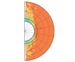Because the distribution of the relative velocity is symmetrical about the z-axis of the spherical coordinate system $({\theta _{\boldsymbol{k}}},|{\boldsymbol{r}_s} - {\boldsymbol{r}_l}|,\varphi )$ shown in figure 3, the x and y components of $\langle \boldsymbol{g}\rangle ({\theta _{\boldsymbol{k}}},|{\boldsymbol{r}_s} - {\boldsymbol{r}_l}|)$ and $\langle \boldsymbol{g}\rangle $ are close to zero. As discussed earlier, a small particle is easily trapped within the space around a large particle, and statistically has a velocity close to that of the large particle. As a result, the regions of the low relative velocity are formed near large particles, as shown in figure 4. As the total solid volume fraction increases, the distance that the trapped small particle is allowed to travel becomes smaller and smaller, and therefore the regions of low relative velocity gradually shrink. In the streamwise direction, the collision force, which hinders the growth of the relative velocity, decreases with ${\theta _{\boldsymbol{k}}}$ approaching ${\rm \pi} /2$, and therefore the relative velocity increases under the action of the gas–particle drag force, as shown in figure 4. The mean free path signified by the dotted line decreases as $\phi $ increases since the collision frequency increases with $\phi $. The modules of the mean relative velocities within the mean free path, denoted by $\langle g\rangle (|{\boldsymbol{r}_s} - {\boldsymbol{r}_l}|< {l_s})$, respectively equal $0.93\langle g\rangle $, $0.88\langle g\rangle $ and $0.78\langle g\rangle $ when $\phi = 0.1$, $0.2$ and $0.3$. With $\langle g\rangle (|{\boldsymbol{r}_s} - {\boldsymbol{r}_l}|< {l_s})$, the predictions of (2.13) will be smaller and hence become closer to the simulation results. However, before doing that, the effect of the anisotropy observed in figure 4 on the particle–particle drag force is first discussed.

Figure 3. Geometry of the left part of a bin in two dimensions, which is denoted by $\Delta A$ and indicated by the shadowed area. Here, ${O_1}$ is the origin of a fixed coordinate system, and ${O_2}$ is the origin of a spherical coordinate system $({\theta _{\boldsymbol{k}}},|{\boldsymbol{r}_s} - {\boldsymbol{r}_l}|,\varphi )$, co-moving with large particles. The z-axis of the spherical coordinate system coincides with the flow direction. The geometry of a bin in three dimensions is obtained by rotating $\Delta A$ around the z-axis.

Figure 4. Contour plot of the relative velocity of particle pairs of different size in a polar coordinate system $({\theta _{\boldsymbol{k}}},|{\boldsymbol{r}_s} - {\boldsymbol{r}_l}|)$. The meanings of ${\theta _{\boldsymbol{k}}}$ and $|{\boldsymbol{r}_s} - {\boldsymbol{r}_l}|$ are described in figure 3. The subscript z denotes the streamwise direction. The dotted line indicates $|{\boldsymbol{r}_s} - {\boldsymbol{r}_l}|= {l_s}$, where ${l_s}$ is the mean free path of small particles and calculated by (4.1) and (4.2). Here, ${x_s} \approx 0.3$, ${d_l}/{d_s} = 2$, $\langle R{e_p}\rangle \approx 70.7$ and (a) $\phi = 0.1$, (b) $\phi = 0.2$, (c) $\phi = 0.3$.

By symmetry, the collision forces cancel each other in the directions perpendicular to the flow direction, and therefore only the streamwise component contributes to the particle–particle drag force. The streamwise component of the collision force varies with the polar angle as the function $\cos {\theta _{\boldsymbol{k}}}$, and consequently the relative velocity also changes as a function of ${\theta _{\boldsymbol{k}}}$, as mentioned above. It is necessary to consider the correlation between the two functions in calculating the particle–particle drag force. For example, the relative velocity is large around ${\theta _{\boldsymbol{k}}} = {\rm \pi}/2$, but the streamwise component of the collision force in this region is close to zero. Therefore, it can be expected that (2.13) will overestimate the particle–particle drag force by neglecting the anisotropic distribution of the relative velocity. A feasible way to consider the correlation is first to compute the particle–particle drag forces at different polar angles and then sum them up. Assuming the single-particle VDF at each polar angle is Maxwellian, the derivation process of the particle–particle drag force at a specific polar angle is given as follows:

(4.3)\begin{align} {\unicode{x1D4BB}_{\!sl}} & ={-} d_{sl}^2\dfrac{{{m_s}{m_l}}}{{{m_s} + {m_l}}}(1 + {e_{sl}}){\chi _{sl}}\iint\!\!\!\int_{\boldsymbol{g}\boldsymbol{\cdot }\boldsymbol{k} > 0} {{f_s}{f_l}{{(\boldsymbol{g}\boldsymbol{\cdot }\boldsymbol{k})}^2}\boldsymbol{k}\,\textrm{d}\boldsymbol{k}\,\textrm{d}{\boldsymbol{c}_l}\,\textrm{d}{\boldsymbol{c}_s}} \nonumber\\ & ={-} d_{sl}^2\dfrac{{{m_s}{m_l}}}{{{m_s} + {m_l}}}(1 + {e_{sl}})\dfrac{{{\chi _{sl}}{n_s}{n_l}}}{{{{(2{\rm \pi} )}^3}{{({T_s}{T_l})}^{3/2}}}}\iint\!\!\!\int_{\boldsymbol{g}\boldsymbol{\cdot }\boldsymbol{k} > 0}\nonumber\\ &\quad \times {{\textrm{e}^{ - {{[{\boldsymbol{c}_s} - {\boldsymbol{u}_s}({\theta _{\boldsymbol{k}}})]}^2}/(2{T_s}) - {{[{\boldsymbol{c}_l} - {\boldsymbol{u}_l}({\theta _{\boldsymbol{k}}})]}^2}/(2{T_l})}}{{(\boldsymbol{g}\boldsymbol{\cdot }\boldsymbol{k})}^2}\boldsymbol{k}\,\textrm{d}\boldsymbol{k}\,\textrm{d}{\boldsymbol{c}_l}\,\textrm{d}{\boldsymbol{c}_s}} . \end{align}

Note that ${\boldsymbol{u}_s}$ and ${\boldsymbol{u}_l}$ vary with ${\theta _{\boldsymbol{k}}}$ in this equation. By the integral method employed in Glansdorff (Reference Glansdorff1962) and Zhao & Wang (Reference Zhao and Wang2020), the above equation can be transformed into

(4.4)\begin{align} {{\unicode{x1D4BB}}_{\!sl}} = C\int {{\textrm{e}^{-({T_s} + {T_l})/(2T_s T_l){{(\boldsymbol{G} - \langle \boldsymbol{G}\rangle )}^2}}}\,\textrm{d}\boldsymbol{G}} \iint_{\boldsymbol{g}\boldsymbol{\cdot }\boldsymbol{k} > 0} {{\textrm{e}^{ - {{[\boldsymbol{g} - \langle \boldsymbol{g}\rangle ({\theta _{\boldsymbol{k}}})]}^2}/(2({T_s} + {T_l}))}}{{(\boldsymbol{g}\boldsymbol{\cdot }\boldsymbol{k})}^2}\boldsymbol{k}\,\textrm{d}\boldsymbol{g}\,\textrm{d}\boldsymbol{k}} ,\end{align}

where $\boldsymbol{G} = ({T_s}{\boldsymbol{c}_l} + {T_l}{\boldsymbol{c}_s})/({T_s} + {T_l})$, and $\textrm{d}{\boldsymbol{c}_l}\,\textrm{d}{\boldsymbol{c}_s} = \textrm{d}\boldsymbol{G}\,\textrm{d}\boldsymbol{g}$ according to the Jacobian determinant. Here, C is the constant before the integral sign of (4.3). The integral of $\boldsymbol{g}$ is carried out in the spherical coordinates where the z-axis coincides with $\boldsymbol{k}$ and is given as

(4.5)\begin{align} {{\unicode{x1D4BB}}_{\!sl}} & = C{\left( {\dfrac{{2{\rm \pi} {T_s}{T_l}}}{{{T_s} + {T_l}}}} \right)^{3/2}}\iint_{\boldsymbol{g}\boldsymbol{\cdot }\boldsymbol{k} > 0} {{\textrm{e}^{ - {{g^{\prime 2}}}/(2({T_s} + {T_l}))}}{{(\boldsymbol{g}\boldsymbol{\cdot }\boldsymbol{k})}^2}\boldsymbol{k}\,\textrm{d}\boldsymbol{g}^{\prime}\,\textrm{d}\boldsymbol{k}} \nonumber\\ & = 2{\rm \pi} C{\left( {\dfrac{{2{\rm \pi} {T_s}{T_l}}}{{{T_s} + {T_l}}}} \right)^{3/2}}\int_{\boldsymbol{g}\boldsymbol{\cdot}\boldsymbol{k} > 0} {{\textrm{e}^{ - {{g^{\prime 2}}}/(2(T_s+T_l))}} {{(g\cos {\theta _{\boldsymbol{g}}})}^2}{{g^{\prime 2}}}\sin {\theta _{\boldsymbol{g^{\prime}}}}\,\textrm{d}{\theta _{\boldsymbol{g^{\prime}}}}\,\textrm{d}g^{\prime}\boldsymbol{k}\,\textrm{d}\boldsymbol{k}} .\end{align}

From $\boldsymbol{g}\boldsymbol{\cdot }\boldsymbol{k} = \textrm{[}\langle \boldsymbol{g}\rangle \textrm{(}{\theta _{\boldsymbol{k}}}\textrm{) + }\boldsymbol{g^{\prime}}]\boldsymbol{\cdot }\boldsymbol{k}$, i.e. $g\cos {\theta _{\boldsymbol{g}}} = \langle g\rangle ({\theta _{\boldsymbol{k}}})\cos {\psi _{\boldsymbol{k}}} + g^{\prime}\cos {\theta _{\boldsymbol{g^{\prime}}}}$, we have that $\boldsymbol{g}\boldsymbol{\cdot }\boldsymbol{k} > 0$ is equivalent to $\cos {\theta _{\boldsymbol{g^{\prime}}}} > - \langle g\rangle ({\theta _{\boldsymbol{k}}})\cos {\psi _{\boldsymbol{k}}}/g^{\prime}$. Here, ${\psi _{\boldsymbol{k}}}$ is the angle between $\langle \boldsymbol{g}\rangle ({\theta _{\boldsymbol{k}}})$ and $\boldsymbol{k}$. Let $x = \cos {\theta _{\boldsymbol{g^{\prime}}}}$, (4.5) is changed into

(4.6) \begin{align}{{\unicode{x1D4BB}}_{\!sl}} &= 2{\rm \pi} C{\left( {\frac{{2{\rm \pi} {T_s}{T_l}}}{{{T_s} + {T_l}}}} \right)^{3/2}}\int_D {{e^{ - {{g^{\prime 2}}}/(2({T_s} + {T_l}))}}} [\langle g\rangle {\textrm{(}{\theta _{\boldsymbol{k}}}\textrm{)}^2}{g^{\prime 2}}{\cos ^2}{\psi _{\boldsymbol{k}}} + {g^{\prime 4}}{x^2}\nonumber\\ &\quad + 2\langle g\rangle \textrm{(}{\theta _{\boldsymbol{k}}}\textrm{)}{g^{\prime 3}}\cos {\psi _{\boldsymbol{k}}}x]\,\textrm{d}x\,\textrm{d}g^{\prime}\boldsymbol{k}\, \textrm{d}\boldsymbol{k}.\end{align}

Here, D is the domain of integration. When $0 < {\psi _{\boldsymbol{k}}} < {\rm \pi}/2$

(4.7) \begin{align}D &= \{ - 1 < x < 1,\,0 < g^{\prime} < \langle g\rangle \textrm{(}{\theta _{\boldsymbol{k}}})\cos {\psi _{\boldsymbol{k}}}\}\nonumber\\ &\quad \cup \left\{ { - \frac{{\langle g\rangle \textrm{(}{\theta_{\boldsymbol{k}}})\cos {\psi_{\boldsymbol{k}}}}}{{g^{\prime}}} < x < 1,\,\langle g\rangle({\theta_{\boldsymbol{k}}})\cos {\psi_{\boldsymbol{k}}} < g^{\prime} < + \infty } \right\}.\end{align}

When ${\rm \pi} /2 < {\psi_{\boldsymbol{k}}} < {\rm \pi}$

(4.8) \begin{equation}D = \left\{ { - \frac{{\langle g\rangle\textrm{(}{\theta_{\boldsymbol{k}}})\cos {\psi_{\boldsymbol{k}}}}}{{g^{\prime}}} < x < 1, - \langle g\rangle \textrm{(}{\theta_{\boldsymbol{k}}})\cos {\psi_{\boldsymbol{k}}} < g^{\prime} < + \infty } \right\}.\end{equation}

Equation (4.6) can be integrated by parts, and it is found that the results in both situations, i.e. $0 < {\psi _{\boldsymbol{k}}} < {\rm \pi}/2$ and ${\rm \pi} /2 < {\psi _{\boldsymbol{k}}} < {\rm \pi}$, are the same

(4.9) \begin{align} {{\unicode{x1D4BB}}_{\!sl}} & ={-} 2{\rm \pi} d_{sl}^2\dfrac{{{m_s}{m_l}}}{{{m_s} + {m_l}}}(1 + {e_{sl}}){n_s}{n_l}({T_s} + {T_l}){\chi _{sl}}\int {\left\{ {\dfrac{1}{{\sqrt {\rm \pi} }}{{\cos }^2}{\theta_{\boldsymbol{k}}}\,{\textrm{e}^{ - {{[\langle {g^\ast }\rangle ({\theta_{\boldsymbol{k}}})\cos {\theta_{\boldsymbol{k}}}]}^2}}}} \right.} \nonumber\\ & \quad +\, \left[ {\dfrac{{\cos {\theta_{\boldsymbol{k}}}}}{{2\langle {g^\ast }\rangle ({\theta_{\boldsymbol{k}}})}} + \langle {g^\ast }\rangle ({\theta_{\boldsymbol{k}}}){{\cos }^3}{\theta_{\boldsymbol{k}}}} \right]erf[\langle {g^\ast }\rangle ({\theta _{\boldsymbol{k}}})\cos {\theta _{\boldsymbol{k}}}]\nonumber\\ & \quad \left. { + \,\dfrac{{A\cos {\theta_{\boldsymbol{k}}}}}{{2\langle {g^\ast }\rangle ({\theta_{\boldsymbol{k}}})}} + A\langle {g^\ast }\rangle ({\theta_{\boldsymbol{k}}}){{\cos }^3}{\theta_{\boldsymbol{k}}}} \right\}\sin {\theta _{\boldsymbol{k}}}\langle {\boldsymbol{g}^\ast }\rangle ({\theta _{\boldsymbol{k}}})\,\textrm{d}{\theta _{\boldsymbol{k}}}, \end{align}

where the integrand function multiplied by $d{\theta _{\boldsymbol{k}}}$ is the particle–particle drag force at ${\theta _{\boldsymbol{k}}}$. In the above equation, $\cos {\psi _{\boldsymbol{k}}}$ is replaced by $\cos {\psi _{\boldsymbol{k}}} = A\cos {\theta _{\boldsymbol{k}}}$ since $\langle \boldsymbol{g}\rangle ({\theta _{\boldsymbol{k}}}\textrm{)}$ is parallel with $\langle \boldsymbol{g}\rangle $. Here, $A = \textrm{1}$ when $\langle \boldsymbol{g}\rangle ({\theta _{\boldsymbol{k}}}\textrm{)}$ is in the direction of $\langle \boldsymbol{g}\rangle $, and $A ={-} \textrm{1}$ when $\langle \boldsymbol{g}\rangle ({\theta _{\boldsymbol{k}}}\textrm{)}$ is in the opposite direction of $\langle \boldsymbol{g}\rangle $.

To compute the particle–particle drag force, the integral in (4.9) is discretized numerically, and the mean of the relative velocity in each discrete interval $\Delta {\theta _{\boldsymbol{k}}}$ within the range $|{\boldsymbol{r}_s} - {\boldsymbol{r}_l}|< {l_s}$, represented by $\langle \boldsymbol{g}\rangle \textrm{(}{\theta _{\boldsymbol{k}}},|{\boldsymbol{r}_s} - {\boldsymbol{r}_l}|< {l_s}\textrm{)}$, is substituted into the discrete equation. Figure 5 shows the comparison between predictions and simulation results for all simulation cases in this study. The square points are computed by substituting the mean of the relative velocity within the range $|{\boldsymbol{r}_s} - {\boldsymbol{r}_l}|< {l_s}$, i.e. $\langle \boldsymbol{g}\rangle \textrm{(}|{\boldsymbol{r}_s} - {\boldsymbol{r}_l}|< {l_s}\textrm{)}$, into (2.13), and therefore do not include the effect of the anisotropy. The predictions by (4.9) are the most accurate with a mean error of $8\,\textrm{%}$ (maximum $25\,\textrm{%}$), and the prediction by (2.13) with $\langle \boldsymbol{g}\rangle $ is the worst with a mean error of $61\,\textrm{%}$ (maximum $109\,\textrm{%}$). The predictions by (2.13) with $\langle \boldsymbol{g}\rangle \textrm{(}|{\boldsymbol{r}_s} - {\boldsymbol{r}_l}|< {l_s}\textrm{)}$ are between the predictions by (2.13) and (4.9) with a mean error of $32\,\textrm{%}$ (maximum $48\,\textrm{%}$), which indicates that the anisotropy of the relative-velocity distribution cannot be neglected. Note that (4.9) still slightly overestimates the particle–particle drag force. This may be caused by hydrodynamic interactions between particle pairs.

Figure 5. Predictions versus simulation results for the particle–particle drag force of small particles. Circles, squares and triangles respectively represent the predictions calculated by (2.13) with $\langle \boldsymbol{g}\rangle $, (2.13) with $\langle \boldsymbol{g}\rangle (|{\boldsymbol{r}_s} - {\boldsymbol{r}_l}|< {l_s})$ and (4.9) with $\langle \boldsymbol{g}\rangle ({\theta _{\boldsymbol{k}}},|{\boldsymbol{r}_s} - {\boldsymbol{r}_l}|< {l_s})$. The dotted line is the bisector line $y = x$. The parameter range is shown in table 1.

To apply (4.9) in MFM simulations, the relative velocity within a mean free path of small particles ${l_s}$, i.e. $\langle \boldsymbol{g}\rangle \textrm{(}{\theta _{\boldsymbol{k}}},|{\boldsymbol{r}_s} - {\boldsymbol{r}_l}|< {l_s}\textrm{)}$, must be adequately resolved, which implies that the grid size should be much smaller than ${l_s}$. For the case shown in figure 4(c), the mean free path is only $1.28{d_{sl}}$, leading to a grid size of a small fraction of a large-particle diameter. It is infeasible to use such a fine grid in MFM simulations mainly due to the huge computational cost. With this in mind, the relative velocity $\langle \boldsymbol{g}\rangle $ in (2.13) is replaced by an effective relative velocity, denoted as $\alpha \langle \boldsymbol{g}\rangle $, in order to make the predictions of (2.13) agree with those of (4.9), that is

(4.10)\begin{equation}{{\unicode{x1D4BB}}_{\!sl}}(\alpha \langle \boldsymbol{g}\rangle ) = {{\unicode{x1D4BB}}_{\!sl}}[\langle \boldsymbol{g}\rangle ({\theta _{\boldsymbol{k}}},|{\boldsymbol{r}_s} - {\boldsymbol{r}_l}|< {l_s})].\end{equation}

The factor $\alpha $ is solved by iteration. With $\phi $ increasing, the probability of repeated collisions increases since the particle motion is more restricted. Consequently, the correlation between pre-collision velocities becomes stronger, and accordingly, the factor $\alpha $ decreases, as seen in figure 6. The effect of ${x_s}$ on $\alpha $ is twofold. First, the effect of ${x_s}$ is the same as the effect of $\phi $ because the total particle number density increases with ${x_s}$. Second, as ${x_s}$ increases, the collisions between small particles become more frequent, and small particles relax more quickly. This is because the collisions between like particles help a post-collision pair to recover their statistically stationary velocities. If the correlation between pre-collision velocities is mainly controlled by the relaxation process of small particles, the correlation becomes weaker and therefore $\alpha $ increases. As shown in figure 6, the factor $\alpha $ decreases with ${x_s}$, which indicates the first effect dominates the correlation between pre-collision velocities. Note that the particle diameter ratio and the Reynolds number have a minor effect on $\alpha $. The factor $\alpha $ is approximately fitted by a linear function of $\phi $ and ${x_s}$, which is given as

(4.11)\begin{equation}\alpha ={-} 1.363\phi - 0.3875{x_s} + 1.089.\end{equation}

The predictions of (2.13) with $\alpha \langle \boldsymbol{g}\rangle $ where $\alpha $ is computed by (4.11) are close to that of (4.9), and deviate from simulation results by $10\,\textrm{%}$ on average ($23\,\textrm{%}$ maximum).

Figure 6. Variation of the factor $\alpha $, defined by (4.10), with the total solid volume fraction $\phi $ at different volume fractions of small particles ${x_s}$. The error bar characterizes the standard deviation derived from the cases of different particle diameter ratios and particle Reynolds numbers. The dotted lines are the fitting curves given by (4.11).

5. Model assessment

In order to assess the performance of the model proposed in this study, we implement the model

(5.1) \begin{align} {\boldsymbol{\unicode{x1D4BB}}_{\!ij}} & ={-} 2{\rm \pi} d_{ij}^2\dfrac{{{m_i}{m_j}}}{{{m_i} + {m_j}}}(1 + {e_{ij}}){n_i}{n_j}({T_i} + {T_j}){\chi _{ij}}\left[ {\dfrac{1}{{\sqrt {\rm \pi} }}\left( {\dfrac{1}{2} + \dfrac{1}{{4{\alpha^2}{{\langle {g^\ast }\rangle }^2}}}} \right)\,{\textrm{e}^{ - {\alpha^2}{{\langle {g^\ast }\rangle }^2}}}} \right.\nonumber\\ & \quad \left. { + \left( {\dfrac{{\alpha \langle {g^\ast }\rangle }}{2} + \dfrac{1}{{2\alpha \langle {g^\ast }\rangle }} - \dfrac{1}{{8{\alpha^3}{{\langle {g^\ast }\rangle }^3}}}} \right)erf(\alpha \langle {g^\ast }\rangle )} \right]\alpha \langle {\boldsymbol{g}^\ast }\rangle \nonumber\\ & \quad \alpha ={-} 1.363\phi - 0.3875{x_s} + 1.089, \end{align}

in MFIX-MFM and perform MFM simulations. The cases of $\phi = 0.1\sim 0.3$, ${x_s} \approx 0.3$, ${d_l}/{d_s} = 2$ and $\langle R{e_p}\rangle \approx 70.7$ are chosen. For comparison, the input parameter settings and boundary conditions are consistent with the PR-DNSs. Assuming the gas is air and the gravitational acceleration equals $9.81\ \textrm{m}\ {\textrm{s}^{ - 2}}$, the input parameters in lattice units are converted into those in physical units and listed in table 2. The gas–particle drag force is calculated by the model of Beetstra et al. (Reference Beetstra, van der Hoef and Kuipers2007), which is appropriate for bidisperse suspensions that are inertial and homogeneous. Benyahia (Reference Benyahia2008) compared the predictions of several kinetic theories with molecular dynamic data and found the kinetic theory of Iddir & Arastoopour (Reference Iddir and Arastoopour2005) is the most accurate one. Consequently, the kinetic theory of Iddir & Arastoopour (Reference Iddir and Arastoopour2005) is adopted in the present study. The grid size of $2.5{d_l}$ is chosen, and it has been found that the domain-averaged quantities do not change as the grid size decreases to $0.5{d_l}$.

Table 2. The input parameter settings for MFM simulations. Here, g is the gravitational acceleration, and $\Delta p$ is the pressure drop across the entire domain, which is used to drive the flow; e and ${C_f}$ represent the coefficient of restitution and the friction coefficient, respectively; t is the total simulation time.

Figure 7. The relative velocity (a), particle–particle drag force of small particles and gas–particle drag force are shown as functions of the total solid volume faction. Here, the relative velocity is non-dimensionalized by the Sauter mean diameter and kinematic viscosity to give the particle Reynold number, and the gas–particle drag force is normalized by the Stokes drag force. The abbreviations ZW, IA and S denote the models of Zhao & Wang (Reference Zhao and Wang2021), Iddir & Arastoopour (Reference Iddir and Arastoopour2005) and Syamlal (Reference Syamlal1987), respectively.

Besides the model of this study and Zhao & Wang (Reference Zhao and Wang2021), the models of Syamlal (Reference Syamlal1987) and Iddir & Arastoopour (Reference Iddir and Arastoopour2005) are also tested. Note that when $\alpha = 1$, (5.1) degenerates to the model of Zhao & Wang (Reference Zhao and Wang2021), i.e. (2.13). The models of Syamlal (Reference Syamlal1987) and Iddir & Arastoopour (Reference Iddir and Arastoopour2005) are respectively given as

(5.2)\begin{gather}{\boldsymbol{\unicode{x1D4BB}}_{\!ij}} ={-} d_{ij}^2\frac{{{m_i}{m_j}}}{{{m_i} + {m_j}}}(1 + {e_{ij}}){n_i}{n_j}{\chi _{ij}}\left( {\frac{{\rm \pi} }{2} + \frac{{{{\rm \pi} ^2}{C_f}}}{8}} \right)\langle g\rangle \langle \boldsymbol{g}\rangle \textrm{,}\end{gather}

(5.3)\begin{gather}{\boldsymbol{\unicode{x1D4BB}}_{\!ij}} ={-} \frac{{\sqrt {\rm \pi} d_{ij}^2}}{4}\frac{{{m_i}{m_j}}}{{{m_i} + {m_j}}}(1 + {e_{ij}}){n_i}{n_j}{\chi _{ij}}{\left( {\frac{1}{{{T_i}{T_j}}}} \right)^{3/2}}{R_2}\langle \boldsymbol{g}\rangle \textrm{,}\end{gather}

(5.4)\begin{gather}{R_2} = \frac{1}{{2A_{ij}^{3/2}D_{ij}^2}} + \frac{{3B_{ij}^2}}{{A_{ij}^{5/2}D_{ij}^3}} + \frac{{15B_{ij}^4}}{{A_{ij}^{7/2}D_{ij}^4}} + \cdots ,\end{gather}

(5.5a–c)\begin{gather}{A_{ij}} = \frac{{{T_i} + {T_j}}}{{2{T_i}{T_j}}},\quad {B_{ij}} = \frac{{{m_j}{T_j} - {m_i}{T_i}}}{{2({m_i} + {m_j}){T_i}{T_j}}},\quad {D_{ij}} = \frac{{m_i^2{T_i} + m_j^2{T_j}}}{{2{{({m_i} + {m_j})}^2}{T_i}{T_j}}}.\end{gather}

In (5.2), the model of Syamlal (Reference Syamlal1987), ${C_f}$ denotes the friction coefficient and equals zero in the present study. And in (5.3), the model of Iddir & Arastoopour (Reference Iddir and Arastoopour2005), the terms including the gradients of the particle number density and granular temperature are neglected because the studied suspensions are homogeneous. In addition, the granular temperature in the paper of Iddir & Arastoopour (Reference Iddir and Arastoopour2005) includes the particle mass, while the granular temperature in this paper, i.e. ${T_i}$, does not.

Figures 7(a), 7(b) and 7(c) respectively plot the dimensionless relative velocity, the particle–particle drag force and the gas–particle drag force as functions of $\phi $. For convenience, the abbreviations ZW, IA and S are introduced to respectively represent the models of Zhao & Wang (Reference Zhao and Wang2021), Iddir & Arastoopour (Reference Iddir and Arastoopour2005) and Syamlal (Reference Syamlal1987). As shown in figure 7(a,b), model S highly underestimates the particle–particle drag force due to neglecting the granular temperature. Consequently, the relative velocity predicted by model S is much higher than that of PR-DNSs. As discussed in this paper, model ZW overpredicts the particle–particle drag force by neglecting the correlation between pre-collision velocities and hence underpredicts the relative velocity. The particle–particle drag force predicted by model IA is reasonably good for $\phi = 0.1$ and $0.2$ but too high for $\phi = 0.3$. In the derivation process of Iddir & Arastoopour (Reference Iddir and Arastoopour2005), the Taylor expansion is applied to the Maxwell distribution function and some simplifications are made, such as the module of the relative velocity $|{\boldsymbol{c}_i} - {\boldsymbol{c}_j}|$ replaced by $|{\boldsymbol{C}_i} - {\boldsymbol{C}_j}|$. The readers can refer to the paper of Zhao & Wang (Reference Zhao and Wang2020) for more details. In fact, model IA should be the same as model ZW if no approximation is made. A comparison between the predictions of model IA and those of model ZW shows that the approximations made by Iddir & Arastoopour (Reference Iddir and Arastoopour2005) are inaccurate. Hence the good agreement of model IA for $\phi = 0.1$ and $0.2$ is just a coincidence. The model proposed in this study shows good agreement for the particle–particle drag force but underpredicts the relative velocity for $\phi = 0.1$ and $0.2$. The reason for this underestimate is due to the inaccuracy of the gas–particle drag model. As shown in figure 7(c), the model of Beetstra et al. (Reference Beetstra, van der Hoef and Kuipers2007) overpredicts the gas–particle drag force of large particles for $\phi = 0.1$ and $0.2$. Since the particle velocity increases with the gas–particle drag force, the large-particle velocity is overestimated, leading to an underestimated relative velocity. This is also the reason why the particle–particle drag forces predicted by model ZW and model IA gradually approach PR-DNSs as $\phi $ decreases while the relative velocities do not show this trend. At $\phi = 0.3$, where the model of Beetstra et al. (Reference Beetstra, van der Hoef and Kuipers2007) is accurate, the relative velocity predicted by the present model is in good agreement with PR-DNSs, verifying the accuracy of the model proposed in this study.