


1 Introduction
Whether flow over delta wings or tornadoes, axial vortices are ubiquitous in engineering and nature. Axial vortices are prone to a phenomenon called ‘vortex breakdown’, first observed by Peckham & Atkinson (Reference Peckham and Atkinson1957) in flow past delta wings. It is characterized by the appearance of one or more stagnation points on or near the axis of the vortex followed by a spiral (spiral-type vortex breakdown) or a re-circulatory bubble (bubble-type vortex breakdown) or a double helix (helical-type vortex breakdown) (Leibovich Reference Leibovich1978; Escudier Reference Escudier1984, Reference Escudier1988; Delery Reference Delery1994). Earliest known observations by Michaud (Reference Michaud1787) documented schematics showing breakdowns in tornadoes and waterspouts, which occur at different stages in the lifecycle (Pauley & Snow Reference Pauley and Snow1988). In hurricanes the vortex breakdown appears as the ‘eye’ which is a silent region, with little being known about the formation process and characterization of the eye. Recently, Sharma & Sameen (Reference Sharma and Sameen2019) have shown that axisymmetric vortex breakdown inhibits mixing by acting as a barrier to fluid transport. In this study we note that the breakdown bubble (defined as  $u_{z}=0$ surface) and planar helicity are correlated.
Helicity is one of the important variables used in the study of rotating flows. It has been used extensively to analyse the stability and the energy propagation in atmospheric flows (Elting Reference Elting1985). Lilly (Reference Lilly1986) has shown that supercell thunderstorms can be categorized with high helicity. Scheeler et al. (Reference Scheeler, Van Rees, Kedia, Kleckner and Irvine2017) have shown that for vortex tubes total helicity can be determined by computing twist, writhe and linking number. In the present analysis we use helicity density to understand vortex breakdown. While helicity is an integral quantity, helicity density is a local quantity, which is given by
 $$\begin{eqnarray}h=\boldsymbol{u}\boldsymbol{\cdot }\unicode[STIX]{x1D74E}.\end{eqnarray}$$
 Helicity density represents the orientation of the velocity vector  $\boldsymbol{u}=(u_{\unicode[STIX]{x1D703}},u_{r},u_{z})$ and the vorticity vector
  $\unicode[STIX]{x1D74E}=(\unicode[STIX]{x1D714}_{\unicode[STIX]{x1D703}},\unicode[STIX]{x1D714}_{r},\unicode[STIX]{x1D714}_{z})$, and, hence, is directly related to the local topology of the flow. Helicity density has been used to understand vortex breakdown in the past. A possible correlation of helicity density with vortex breakdown was first discussed briefly by Moffatt & Tsinober (Reference Moffatt and Tsinober1992), arguing that vortex breakdown is a result of the change in the topology of the flow and helicity may be a suitable parameter to characterize it. Spall & Gatski (Reference Spall and Gatski1990) have used helicity density to analyse vortex breakdown in rotating pipe flows while Yoshizawa et al. (Reference Yoshizawa, Yokoi, Nisizima, Itoh and Itoh2001) used helicity density to show that the axial vorticity component plays a central role in flow reversal at the axis for swirling pipe flow. The fact that helicity density changes sign across a separation or reattachment line makes it a suitable parameter for predicting the stagnation points which precede vortex breakdown.
To study the vortex breakdown phenomenon, we have used a model problem that generates bubble-type vortex breakdown. Bubble-type vortex breakdown is generated inside a circular cylinder with a rotating top lid, henceforth called Vogel–Escudier flow (Vogel Reference Vogel1968; Escudier Reference Escudier1984; Shtern Reference Shtern2018). Two non-dimensional parameters that govern the flow are: (i) aspect ratio,  $\unicode[STIX]{x1D6E4}=H/R$, where
  $H$ and
  $R$ are the height and radius of the cylinder, and (ii) Reynolds number,
  $Re=\unicode[STIX]{x1D6FA}R^{2}/\unicode[STIX]{x1D708}$, where
  $\unicode[STIX]{x1D6FA}$ is the rate at which the lid is rotated and
  $\unicode[STIX]{x1D708}$ is kinematic viscosity. The number of breakdown bubbles depends on the aspect ratio of the cylinder and the Reynolds number of the flow. Vogel (Reference Vogel1968) presented a map of the number of vortex breakdown bubbles in the
  $\unicode[STIX]{x1D6E4}{-}Re$ plane. Escudier (Reference Escudier1984) extended this map for several combinations of
  $\unicode[STIX]{x1D6E4}$ and
  $Re$ suggesting steady and unsteady regimes in the map along with the number of breakdown bubbles. Brown & Lopez (Reference Brown and Lopez1990) discussed the conditions under which vortex breakdown occurs and proposed that the generation of negative azimuthal vorticity is an essential feature of vortex breakdown. Spall & Gatski (Reference Spall and Gatski1990) have shown that axial vorticity redistributes itself to the other two components of vorticity in the event of vortex breakdown. Wang & Rusak (Reference Wang and Rusak1997) and Shtern & Hussain (Reference Shtern and Hussain1999) have explained vortex breakdown as a fold catastrophe that occurs in rotating pipe flow. Paterson, Wang & Mao (Reference Paterson, Wang and Mao2018) have conducted stability analysis of bubble-type vortex breakdown of an unconfined vortex. Several proposed mechanisms of vortex breakdown can be found elsewhere (Sarpkaya Reference Sarpkaya1971; Leibovich Reference Leibovich1978; Escudier & Keller Reference Escudier and Keller1983; Escudier Reference Escudier1988; Brown & Lopez Reference Brown and Lopez1990; Delery Reference Delery1994; Goldshtik & Hussain Reference Goldshtik and Hussain1998; Shtern & Hussain Reference Shtern and Hussain1999; Hiejima Reference Hiejima2018). Vishnu & Sameen (Reference Vishnu and Sameen2019) have investigated thermally unstable stratified Vogel–Escudier flow and observed that the large-scale circulation is affected by the breakdown bubble. The heat transfer increases with an increase in the Reynolds number, which is the result of enhanced upward flow at the bottom hot plate that assists the convection.
Helicity density can be decomposed as given in Biferale, Buzzicotti & Linkmann (Reference Biferale, Buzzicotti and Linkmann2017) to analyse the flow. When the physics of the flow is dominated by the dynamics in the two-dimensional (2-D) plane it is shown that the three-dimensional (3-D) flow can be written as the sum of the velocity vector in the 2-D plane and an out-of-plane velocity vector. This kind of decomposition is common for analysing transition from 2-D to 3-D turbulence. In this paper we have scenarios of a similar transition from axisymmetric to non-axisymmetric flow and the flow field is decomposed as two-dimensional three-component (2D3C) flow.
The paper is organized as follows. The numerical method is presented in § 2 along with the validation and streamline plots of the flow for various Reynolds numbers in the  $rz$ plane. Helicity density of the flow and the change in its sign associated with vortex breakdown are examined and discussed in § 3. Section 4 presents the decomposition of the 3-D velocity field into the sum of 2-D flow in the
  $rz$ plane and an out-of-plane component. An analytical expression for planar helicity, using this decomposed 2D3C velocity field, is also presented in that section. A correlation between planar helicity density and the breakdown bubble boundary is shown by order-of-magnitude analysis. This concurrence between the planar helicity and the vortex breakdown bubbles (axisymmetric as well as non-axisymmetric) is also shown by plotting planar helicity alongside the breakdown bubble in that section. Planar helicity is further used to reconstruct 3-D non-axisymmetric vortex breakdown bubbles for
  $\unicode[STIX]{x1D6E4}=2.5$ at
  $Re=5000$. The paper concludes with a discussion about the correlation of planar helicity with vortex breakdown in § 5.
2 Numerical method
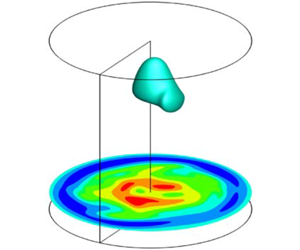
A schematic of the computational domain for Vogel–Escudier flow is shown in figure 1. The top wall of the cylinder is rotated at an angular speed  $\unicode[STIX]{x1D6FA}$. Vogel–Escudier flow is simulated numerically by solving 3-D incompressible Navier–Stokes equations in cylindrical polar coordinate system
  $(\unicode[STIX]{x1D703},r,z)$, which are written in an expanded form (Verzicco & Orlandi Reference Verzicco and Orlandi1996):
 $$\begin{eqnarray}\frac{\unicode[STIX]{x2202}q_{r}}{\unicode[STIX]{x2202}r}+\frac{\unicode[STIX]{x2202}q_{\unicode[STIX]{x1D703}}}{\unicode[STIX]{x2202}\unicode[STIX]{x1D703}}+r\frac{\unicode[STIX]{x2202}q_{z}}{\unicode[STIX]{x2202}z}=0,\end{eqnarray}$$
 $$\begin{eqnarray}\displaystyle \frac{\unicode[STIX]{x2202}q_{\unicode[STIX]{x1D703}}}{\unicode[STIX]{x2202}t}+\frac{1}{r}\frac{\unicode[STIX]{x2202}\left(q_{\unicode[STIX]{x1D703}}q_{\unicode[STIX]{x1D703}}\right)}{\unicode[STIX]{x2202}\unicode[STIX]{x1D703}}+\frac{1}{r^{2}}\frac{\unicode[STIX]{x2202}(rq_{\unicode[STIX]{x1D703}}q_{r})}{\unicode[STIX]{x2202}r}+\frac{\unicode[STIX]{x2202}(q_{\unicode[STIX]{x1D703}}q_{z})}{\unicode[STIX]{x2202}z} & = & \displaystyle -\frac{1}{r}\frac{\unicode[STIX]{x2202}p}{\unicode[STIX]{x2202}\unicode[STIX]{x1D703}}+\frac{1}{Re}\left[\frac{1}{r}\left(\frac{\unicode[STIX]{x2202}}{\unicode[STIX]{x2202}r}r\frac{\unicode[STIX]{x2202}q_{\unicode[STIX]{x1D703}}}{\unicode[STIX]{x2202}r}\right)-\frac{q_{\unicode[STIX]{x1D703}}}{r^{2}}\right.\nonumber\\ \displaystyle & & \displaystyle +\left.\frac{1}{r^{2}}\frac{\unicode[STIX]{x2202}^{2}q_{\unicode[STIX]{x1D703}}}{\unicode[STIX]{x2202}\unicode[STIX]{x1D703}^{2}}+\frac{\unicode[STIX]{x2202}^{2}q_{\unicode[STIX]{x1D703}}}{\unicode[STIX]{x2202}z^{2}}+\frac{2}{r^{3}}\frac{\unicode[STIX]{x2202}q_{r}}{\unicode[STIX]{x2202}\unicode[STIX]{x1D703}}\right],\end{eqnarray}$$
 $$\begin{eqnarray}\displaystyle & & \displaystyle \frac{\unicode[STIX]{x2202}q_{r}}{\unicode[STIX]{x2202}t}+\frac{\unicode[STIX]{x2202}}{\unicode[STIX]{x2202}\unicode[STIX]{x1D703}}\left(\frac{q_{\unicode[STIX]{x1D703}}q_{r}}{r}\right)+\frac{\unicode[STIX]{x2202}}{\unicode[STIX]{x2202}r}\left(\frac{q_{r}q_{r}}{r}\right)+\frac{\unicode[STIX]{x2202}(q_{r}q_{z})}{\unicode[STIX]{x2202}z}-q_{\unicode[STIX]{x1D703}}^{2}\nonumber\\ \displaystyle & & \displaystyle \quad =-r\frac{\unicode[STIX]{x2202}p}{\unicode[STIX]{x2202}r}+\frac{1}{Re}\left[r\frac{\unicode[STIX]{x2202}}{\unicode[STIX]{x2202}r}\left(\frac{1}{r}\frac{\unicode[STIX]{x2202}q_{r}}{\unicode[STIX]{x2202}r}\right)+\frac{1}{r^{2}}\frac{\unicode[STIX]{x2202}^{2}q_{r}}{\unicode[STIX]{x2202}\unicode[STIX]{x1D703}^{2}}+\frac{\unicode[STIX]{x2202}^{2}q_{r}}{\unicode[STIX]{x2202}z^{2}}-\frac{2}{r}\frac{\unicode[STIX]{x2202}q_{\unicode[STIX]{x1D703}}}{\unicode[STIX]{x2202}\unicode[STIX]{x1D703}}\right],\end{eqnarray}$$
 $$\begin{eqnarray}\displaystyle \frac{\unicode[STIX]{x2202}q_{z}}{\unicode[STIX]{x2202}t}+\frac{1}{r}\frac{\unicode[STIX]{x2202}\left(q_{\unicode[STIX]{x1D703}}q_{z}\right)}{\unicode[STIX]{x2202}\unicode[STIX]{x1D703}}+\frac{1}{r}\frac{\unicode[STIX]{x2202}(q_{r}q_{z})}{\unicode[STIX]{x2202}r}+\frac{\unicode[STIX]{x2202}(q_{z}q_{z})}{\unicode[STIX]{x2202}z} & = & \displaystyle -\frac{\unicode[STIX]{x2202}p}{\unicode[STIX]{x2202}z}+\frac{1}{Re}\left[\frac{1}{r}\frac{\unicode[STIX]{x2202}}{\unicode[STIX]{x2202}r}\left(r\frac{\unicode[STIX]{x2202}q_{z}}{\unicode[STIX]{x2202}r}\right)\right.\nonumber\\ \displaystyle & & \displaystyle +\left.\frac{1}{r^{2}}\frac{\unicode[STIX]{x2202}^{2}q_{z}}{\unicode[STIX]{x2202}\unicode[STIX]{x1D703}^{2}}+\frac{\unicode[STIX]{x2202}^{2}q_{z}}{\unicode[STIX]{x2202}z^{2}}\right].\end{eqnarray}$$
 Here  $(q_{\unicode[STIX]{x1D703}},q_{r},q_{z})=(u_{\unicode[STIX]{x1D703}},ru_{r},u_{z})$ is velocity and
  $p$ is pressure. All the lengths are non-dimensionalized using radius,
  $R$, and all the velocity components are non-dimensionalized using the maximum azimuthal velocity of the top lid,
  $\unicode[STIX]{x1D6FA}R$. These two scales give time scale as
  $1/\unicode[STIX]{x1D6FA}$ and pressure scale as
  $\unicode[STIX]{x1D70C}\unicode[STIX]{x1D6FA}^{2}R^{2}$, which are used to non-dimensionalize the respective variables. The density of the fluid is denoted by
  $\unicode[STIX]{x1D70C}$.
A finite-difference method employing a fractional-step algorithm is used to solve the above equations on a fully staggered arrangement. A fully staggered arrangement of variables helps to achieve a better coupling between the pressure and the velocity and reduces oscillations in the solution. It provides another advantage in that at the axis  $(r=0)$ only
  $ru_{r}$ is available and is zero, which avoids a singularity at the axis. Further details of the numerical method can be found in Verzicco & Orlandi (Reference Verzicco and Orlandi1996), Orlandi (Reference Orlandi2000) and Sharma & Sameen (Reference Sharma and Sameen2019). The boundary conditions at the lower wall and side wall are
  $u_{\unicode[STIX]{x1D703}}=u_{r}=u_{z}=0$, and at upper wall are
  $u_{\unicode[STIX]{x1D703}}=r/R,u_{r}=u_{z}=0$. Steady-state cases are started from zero initial conditions and take roughly 500 non-dimensional time units to settle down. For faster convergence, the high-Reynolds-number (unsteady) cases are started using the converged lower
  $Re$ steady-state solution as the initial conditions.

Figure 1. Schematic diagram of the computational domain. The schematic also shows vortex breakdown bubbles represented by isosurface of  $u_{z}=0$ and contours of
  $u_{z}$ in the
  $rz$ plane for
  $Re=2200$ and
  $\unicode[STIX]{x1D6E4}=2.5$. The radial,
  $r$, and axial,
  $z$, coordinates are also shown.
When the top lid is rotated, the fluid adjacent to the lid is pushed outward under the action of centrifuge. Upon reaching the radial wall, the flow descends down along the wall. When the flow reaches the non-rotating bottom wall, it turns radially inward and converges at the axis, where flow is forced to move up towards the top rotating lid to satisfy mass conservation. This phenomenon is also known as Ekman pumping or Ekman suction (Greenspan Reference Greenspan1969; Serre & Bontoux Reference Serre and Bontoux2002). This mechanism sets up a re-circulatory flow in the  $rz$ plane (meridional plane) simultaneously rotating in the
  $\unicode[STIX]{x1D703}$ direction (poloidal plane) driven by the top rotating lid and produces a slender axial vortex at the axis. This axial vortex breaks down beyond some critical value of Reynolds number forming what is known as bubble-type vortex breakdown.
2.1 Grid independence study and validation
A grid independence study is done for the cases that are considered in this study. For this purpose solutions for  $Re=2200$ and 5000 for
  $\unicode[STIX]{x1D6E4}=2.5$ are simulated for three different grids. Maximum and minimum values of axial and radial components of the velocity field in the domain are compared for these three grids. Grid dependency for both the Reynolds numbers is shown in table 1. The results are checked for consistency with both constant Courant–Friedrichs–Lewy number and constant time-step
  $(\unicode[STIX]{x0394}t)$ calculations and the results in the table 1 are presented for
  $\unicode[STIX]{x0394}t=10^{-3}$. Differences in the maximum and minimum values for
  $G2$ (
 $257\times 129\times 257$) and
  $G3$ (
 $385\times 197\times 385$) grids are within
  $5\,\%$ for both the Reynolds numbers. Hence,
  $G2$ is used for all the results of
  $\unicode[STIX]{x1D6E4}=2.5$ in this paper. Results presented in this study are simulated for a fixed time step,
  $\unicode[STIX]{x0394}t=10^{-3}$.
Table 1. Grid dependence study for  $\unicode[STIX]{x1D6E4}=2.5$ for
  $Re=2200$ and
  $Re=5000$. Maximum and minimum contour values in the domain have been compared for three different grids for axial and radial components of the velocity.


Figure 2. Present computational result for  $\unicode[STIX]{x1D6E4}=2.5$ and
  $Re=2200$ compared against experimental results of Fujimura et al. (Reference Fujimura, Yoshizawa, Iwatsu, Koyama and Hyun2001). (a) Axial variation of
  $u_{z}$ at the axis
  $(r=0)$. (b) Radial variation of
  $u_{z}$ at two different axial locations.
Flow has been simulated for various aspect ratios but mainly the results for  $\unicode[STIX]{x1D6E4}=2.5$ have been discussed and described in detail. This particular aspect ratio has been examined experimentally (Escudier Reference Escudier1984; Fujimura et al. Reference Fujimura, Yoshizawa, Iwatsu, Koyama and Hyun2001) as well as computationally (Lopez & Perry Reference Lopez and Perry1992; Stevens, Lopez & Cantwell Reference Stevens, Lopez and Cantwell1999; Blackburn & Lopez Reference Blackburn and Lopez2000). Results for
  $\unicode[STIX]{x1D6E4}=2.5$ and
  $Re=2200$ are compared quantitatively with experimental data of Fujimura et al. (Reference Fujimura, Yoshizawa, Iwatsu, Koyama and Hyun2001) in figure 2. Comparison of axial variation of
  $u_{z}$ at the axis is shown in figure 2(a). Variation of
  $u_{z}$ and the locations of four stagnation points, which are indicated by intersection of the
  $u_{z}$ profile with the axis, match well with the experimental data. Figure 2(b) shows comparison of radial variation of
  $u_{z}$ at two different axial locations (
 $z^{\ast }=z/H=0.924$ and 0.942). Further, the streamline patterns in the
  $rz$ plane for various aspect ratios at
  $Re=2000$ are shown in figure 3. The number of breakdown bubbles matches well with the existing literature (Escudier Reference Escudier1984; Lopez Reference Lopez1990); for higher aspect ratios
  $\unicode[STIX]{x1D6E4}\gtrsim 2.5$ at
  $Re=2000$, there is no vortex breakdown.

Figure 3. Streamlines in the  $rz$ plane at
  $Re=2000$ for (a)
  $\unicode[STIX]{x1D6E4}=1.5$, (b)
  $\unicode[STIX]{x1D6E4}=2.5$ and (c)
  $\unicode[STIX]{x1D6E4}=3$. The flow is steady and axisymmetric for all cases.

Figure 4. Streamlines in the  $rz$ plane for
  $\unicode[STIX]{x1D6E4}=2.5$ for various Reynolds numbers: (a)
  $Re=1000$, (b)
  $Re=1500$, (c)
  $Re=1800$, (d)
  $Re=1900$, (e)
  $Re=2000$, (f)
  $Re=2200$, (g)
  $Re=2494$, (h)
  $Re=2700$ and (i)
  $Re=5000$. The flow is unsteady for the cases shown in (h) and (i) and the streamlines are shown at an instant.
2.2 Vortex breakdown topology for  $\unicode[STIX]{x1D6E4}=2.5$

The flow topology, for  $\unicode[STIX]{x1D6E4}=2.5$, represented by the streamlines in the
  $rz$ plane are shown in figure 4 for various Reynolds numbers. At low
  $Re$ there is no vortex breakdown bubble and the curvature of the streamlines is small near the axis as can be seen in figure 4(a). The streamlines start to have noticeable curvature in the vicinity of the axis of the cylinder near the top rotating lid at
  $Re=1500$, even though there is no vortex breakdown. This curvature is more pronounced at
  $Re=1800$ and is shifted near the bottom stationary lid as shown in figure 4(c). When breakdown occurs and the flow is axisymmetric (figure 4d–h), the streamlines are closed at the axis and breakdown bubbles are visible. The flow is steady and axisymmetric for figure 4(d–g) and has two vortex breakdown bubbles. This result agrees qualitatively with the experimental observations of Escudier (Reference Escudier1984) in terms of the axisymmetric nature of the flow and the number of breakdown bubbles. Similar plots are also presented by Lopez & Perry (Reference Lopez and Perry1992) from axisymmetric computations for
  $\unicode[STIX]{x1D6E4}=2.5$. At
  $Re=2700$, the flow is unsteady and axisymmetric with a large breakdown bubble oscillating along the axis periodically. The breakdown bubble at an instant is shown in figure 4(h). At a higher Reynolds number such as
  $Re=5000$, the flow is non-axisymmetric and from the streamline pattern shown in figure 4(i) it is difficult to estimate the shape and size of the breakdown bubble. To overcome this difficulty,
  $u_{z}=0$ isosurface is used in this paper to represent the breakdown bubble as has been previously used by Serre & Bontoux (Reference Serre and Bontoux2002). In figure 5(a), the difference in size of the bubbles represented by streamlines and isosurface of
  $u_{z}=0$ is visible. Figure 5(b) shows the streamlines at the same instant as in figure 4(i) along with breakdown bubbles represented by
  $u_{z}=0$ isosurface. The breakdown bubbles capturing the essential features such as shape, size and stagnation points are well represented by isosurface of
  $u_{z}=0$.

Figure 5. (a) Two-dimensional streamlines in the  $rz$ plane and
  $u_{z}=0$ isosurface for
  $Re=2200$. (b) Three-dimensional streamlines and
  $u_{z}=0$ isosurface for
  $Re=5000$. Aspect ratio for both plots is
  $\unicode[STIX]{x1D6E4}=2.5$.
Using the isosurface of  $u_{z}=0$, the changes in the flow for
  $\unicode[STIX]{x1D6E4}=2.5$ as
  $Re$ is increased are shown in figure 6. At
  $Re=2700$ (figure 6b), flow exhibits unsteady behaviour but remains axisymmetric and a large breakdown bubble starts oscillating along the axis. This observation from 3-D simulation is in agreement with axisymmetric computations by Lopez & Perry (Reference Lopez and Perry1992). At higher Reynolds number, flow becomes non-axisymmetric as a result of the appearance of multiple azimuthal rotating waves. This case is shown in figure 6(c), where non-axisymmetry of the flow can be seen in the
  $u_{z}$ contours plotted in the
  $z$ plane for
  $Re=5000$.

Figure 6. Contours of  $u_{z}$ in the
  $z$ plane at
  $z=0.1$ and isosurface of
  $u_{z}=0$ for (a)
  $Re=2200$, (b)
  $Re=2700$ and (c)
  $Re=5000$ at an instant for
  $\unicode[STIX]{x1D6E4}=2.5$.

Figure 7. Contours of azimuthal vorticity in the  $rz$ plane for
  $\unicode[STIX]{x1D6E4}=2.5$ at (a)
  $Re=1600$ and (b)
  $Re=2200$.
3 Helicity density of the flow
Brown & Lopez (Reference Brown and Lopez1990) have shown that for axisymmetric vortex breakdowns in Vogel–Escudier flow, the flow far away from the breakdown bubble and the walls can be assumed inviscid. Under this assumption they have shown that in order to have stagnation points on the axis and hence the breakdown bubble, generation of the negative azimuthal vorticity is required in the vicinity of the axis. Contours of azimuthal vorticity in the  $rz$ plane for
  $\unicode[STIX]{x1D6E4}=2.5$, for two different Reynolds numbers, are shown in figure 7. Contours for
  $Re=1600$, which does not have a vortex breakdown, are shown in figure 7(a). Negative azimuthal vorticity can be seen concentrated near the axis. Figure 7(b) shows the contours for
  $Re=2200$, which exhibits two distinct vortex breakdown bubbles. For this case also, negative azimuthal vorticity, stronger than that for
  $Re=1600$, is concentrated in the vicinity of the axis. This indicates that even though negative azimuthal vorticity generation is essential to vortex breakdown, its mere presence does not guarantee vortex breakdown.

Figure 8. Contours of helicity density,  $h$, for
  $\unicode[STIX]{x1D6E4}=2.5$ at (a)
  $Re=1600$ and (b)
  $Re=2200$. Variation of
  $h$ along the axis for (a,b) is shown in (c). The inset shows a zoomed-in view of the variation near the stagnation points. The grey region in (b) is the vortex breakdown bubble represented by isosurface of
  $u_{z}=0$.
We analyse helicity density (1.1) of the flow with bubble-type vortex breakdown in detail in the following discussion. Helicity density contours for  $Re=1600$ and 2200 are shown in figures 8(a) and 8(b), respectively. It can be seen that there is no change in sign of helicity density in the vicinity of the axis in the absence of vortex breakdown (i.e. for
  $Re=1600$), while helicity density is negative in the region where vortex breakdown has formed (
 $Re=2200$) (Sarasija Reference Sarasija2014). Figure 8(c) shows the variation of
  $h$ along the axis of the cylinder for
  $Re=1600$ and 2200. In the case of
  $Re=1600$, since there is no stagnation point on the axis, helicity density does not change sign along the axis. At
  $Re=2200$, there are four stagnation points on the axis and figure 8(c) shows that helicity density changes sign exactly at these four points. It has been observed that helicity density is negative inside as well as in the near vicinity of the breakdown bubbles and is enveloped by positive helicity density. The breakdown bubble is a surface
  $(u_{z}=0)$ across which circulation of the flow changes direction. The bulk clockwise circulation induces an upward flow outside the breakdown bubble. Similarly, a counterclockwise circulation within the breakdown bubble induces a downward flow within the breakdown bubble at the axis. Also note in figure 8(b) that the negative region of helicity density does not match with the vortex breakdown bubble shown by grey contours of
  $u_{z}=0$, except at the stagnation points on the axis. This is true for others cases also, as seen in a sample set shown in figure 9, for three different aspect ratios.

Figure 9. Instantaneous contours of helicity density in the  $rz$ plane compared with the vortex breakdown bubbles represented by
  $u_{z}=0$ (shown by grey region) for three different cases: (a)
  $\unicode[STIX]{x1D6E4}=1.75$ at
  $Re=1850$, (b)
  $\unicode[STIX]{x1D6E4}=3$ at
  $Re=2500$ and (c)
  $\unicode[STIX]{x1D6E4}=4$ at
  $Re=4000$.
The negative helicity density is generated always near the top rotating wall and is transported into the bulk by axial velocity which can be understood by examining the helicity density evolution equation. The evolution equation of helicity density,  $h$, in Cartesian coordinates can be shown to be
 $$\begin{eqnarray}\frac{\unicode[STIX]{x2202}h}{\unicode[STIX]{x2202}t}+u_{j}\frac{\unicode[STIX]{x2202}h}{\unicode[STIX]{x2202}x_{j}}=-\unicode[STIX]{x1D714}_{i}\frac{\unicode[STIX]{x2202}p}{\unicode[STIX]{x2202}x_{i}}+\unicode[STIX]{x1D714}_{j}\frac{\unicode[STIX]{x2202}}{\unicode[STIX]{x2202}x_{j}}\left(\frac{u_{i}^{2}}{2}\right)+\frac{1}{Re}\left(\frac{\unicode[STIX]{x2202}^{2}h}{\unicode[STIX]{x2202}x_{j}^{2}}-2\frac{\unicode[STIX]{x2202}u_{i}}{\unicode[STIX]{x2202}x_{j}}\frac{\unicode[STIX]{x2202}\unicode[STIX]{x1D714}_{i}}{\unicode[STIX]{x2202}x_{j}}\right).\end{eqnarray}$$
 This equation can be rewritten and integrated for the whole volume ![]() (applying Gauss theorem for thetransport term) as
(applying Gauss theorem for thetransport term) as
Following Yoshizawa et al. (Reference Yoshizawa, Yokoi, Nisizima, Itoh and Itoh2001) for pipe flow, the second term on the right-hand side for the Vogel–Escudier flow results in the following form near bottom and top walls:
 $$\begin{eqnarray}\int _{S}\hat{n}\cdot (-hu_{j})\,\text{d}S\approx \int _{S}u_{z}h\,\text{d}S.\end{eqnarray}$$
 Surface  $S$ is parallel to top and bottom walls. This term shows that helicity, which is generated at the top rotating plate, is injected in the bulk flow by the axial component of velocity. Figures 10(a) and 10(b) show the variation of
  $\langle u_{z}h\rangle$ with Reynolds number at the top and bottom plates, respectively. The angle brackets
  $\langle \cdot \rangle$ indicate spatial average in the
  $r{-}\unicode[STIX]{x1D703}$ plane. The helicity density transport increases with Reynolds number at both the plates but the contribution from the bottom plate is negligibly small compared to the top plate. For low values of Reynolds number, the correlation
  $\langle u_{z}h\rangle _{t}$ is very small suggesting that from the top plate the helicity is not transported into the bulk. At large
  $Re$, the correlation becomes strong enough to inject the helicity generated at the top plate through axial velocity.

Figure 10. Variation of  $\langle u_{z}h\rangle$ at (a) the top plate and (b) the bottom plate with respect to
  $Re$. Subscript ‘
 $t$’ refers to the top plate and subscript ‘
 $b$’ refers to the bottom plate.
Presence of non-zero helicity has a significant effect on the dynamics of the flow. As discussed by Moffatt & Tsinober (Reference Moffatt and Tsinober1992), helicity density and the Lamb vector  $(\boldsymbol{u}\times \unicode[STIX]{x1D74E})$ form an identity:
 $$\begin{eqnarray}\frac{|\boldsymbol{u}\times \unicode[STIX]{x1D74E}|^{2}}{|\boldsymbol{u}|^{2}|\unicode[STIX]{x1D74E}|^{2}}+\frac{|\boldsymbol{u}\boldsymbol{\cdot }\unicode[STIX]{x1D74E}|^{2}}{|\boldsymbol{u}|^{2}|\unicode[STIX]{x1D74E}|^{2}}=1.\end{eqnarray}$$
The identity (3.4) indicates that as the magnitude of helicity density increases in the flow, the magnitude of the Lamb vector is bound to decrease. This reduction in the magnitude of the Lamb vector results in the reduction of nonlinearity of the flow (Lugt Reference Lugt1996). The second term of the identity (3.4), relative helicity density, is associated with the local curvature of streamlines in the flow (Levy, Degani & Seginer Reference Levy, Degani and Seginer1990), which is the cosine of the angle between the velocity and the vorticity vectors indicating the degree of alignment of the two vectors.

Figure 11. Contours of vortex breakdown bubble represented by  $u_{z}=0$ and the relative helicity density for
  $\unicode[STIX]{x1D6E4}=2.5$,
  $Re=2200$. Colour contours represent relative helicity density and the line contours show
  $u_{z}=0$.
Figure 11 shows contours of relative helicity density for  $\unicode[STIX]{x1D6E4}=2.5$ at
  $Re=2200$. It shows two distinct regions of negative helicity density in the vicinity of the breakdown bubbles (solid curves). The regions of maximum helicity density have minimum local curvature of the streamlines and vice versa. It can be observed from figure 11 that in the vicinity of the breakdown bubble, relative helicity density is negative indicating that the velocity vector and the vorticity vector are anti-correlated in these regions. However, negative relative helicity density does not conform to the vortex breakdown bubble as shown in the figure.
Decomposition of helicity density into planar helicity and out-of-plane helicity indicates a strong correlation between the breakdown bubble and the negative planar helicity, which is discussed in the next section.
4 Planar helicity density $(h_{r,z})$

A 2D3C decomposition is generally used to analyse 2-D turbulent flows (Biferale et al. Reference Biferale, Buzzicotti and Linkmann2017). In a 2D3C flow, the velocity field can be thought of as an out-of-plane component being advected in a 2-D in-plane flow, such that the 3-D velocity field is decomposed as  $\boldsymbol{u}=\boldsymbol{V}^{2D}+\unicode[STIX]{x1D753}$. In cylindrical polar coordinates
  $\boldsymbol{V}^{2D}=(0,u_{r},u_{z})$ is the 2-D in-plane (
 $rz$-plane) component and
  $\unicode[STIX]{x1D753}=(u_{\unicode[STIX]{x1D703}},0,0)$ is the out-of-plane component. Evolutions of these two velocity components are governed by the following equations:
 $$\begin{eqnarray}\displaystyle & \displaystyle \frac{\unicode[STIX]{x2202}\boldsymbol{V}^{2D}}{\unicode[STIX]{x2202}t}+(\boldsymbol{u}\boldsymbol{\cdot }\unicode[STIX]{x1D735})\boldsymbol{V}^{2D}=-\unicode[STIX]{x1D735}p+\unicode[STIX]{x1D708}\unicode[STIX]{x1D6FB}^{2}\boldsymbol{V}^{2D}, & \displaystyle\end{eqnarray}$$
 $$\begin{eqnarray}\displaystyle & \displaystyle \frac{\unicode[STIX]{x2202}\unicode[STIX]{x1D753}}{\unicode[STIX]{x2202}t}+(\boldsymbol{u}\boldsymbol{\cdot }\unicode[STIX]{x1D735})\unicode[STIX]{x1D753}=\unicode[STIX]{x1D708}\unicode[STIX]{x1D6FB}^{2}\unicode[STIX]{x1D753}. & \displaystyle\end{eqnarray}$$
 The evolution equation for  $\unicode[STIX]{x1D753}$ is coupled to (4.1) through the term
  $u_{\unicode[STIX]{x1D703}}u_{r}/r$. Equations (4.1) and (4.2) are shown here for completeness and are not used to compute any quantity in the paper. The results presented in the discussion are extracted from the velocity field obtained by solving (2.1)–(2.4). Volume-averaged energies in the
  $rz$ plane,
  $\langle E^{2D}\rangle$, and in the out-of-plane component,
  $\langle E^{\unicode[STIX]{x1D703}}\rangle$, are defined as
These components of energy are shown in figure 12 as a function of Reynolds number for  $\unicode[STIX]{x1D6E4}=2.5$, indicating the energy contents associated with the decomposed velocity fields are well separated and hence the 2D3C decomposition is justified. Vorticity fields associated with 2D3C flow are
  $\unicode[STIX]{x1D74E}^{2D}$ and
  $\unicode[STIX]{x1D74E}^{\unicode[STIX]{x1D719}}$, which can be shown as follows:
 $$\begin{eqnarray}\unicode[STIX]{x1D74E}^{2D}=\left\langle \frac{\unicode[STIX]{x2202}u_{r}}{\unicode[STIX]{x2202}z}-\frac{\unicode[STIX]{x2202}u_{z}}{\unicode[STIX]{x2202}r},0,0\right\rangle ;\quad \unicode[STIX]{x1D74E}^{\unicode[STIX]{x1D719}}=\left\langle 0,-\frac{\unicode[STIX]{x2202}u_{\unicode[STIX]{x1D703}}}{\unicode[STIX]{x2202}z},\frac{u_{\unicode[STIX]{x1D703}}}{r}+\frac{\unicode[STIX]{x2202}u_{\unicode[STIX]{x1D703}}}{\unicode[STIX]{x2202}r}\right\rangle .\end{eqnarray}$$
 Here, we are interested in decomposition of helicity density in the  $rz$ plane for the 2D3C flow defined above. Helicity density in the
  $rz$ plane,
  $h_{r,z}$ (referred to as planar helicity from now on), which is associated with
  $\boldsymbol{V}^{2D}$ is then given by
 $$\begin{eqnarray}h_{r,z}=\boldsymbol{V}^{2D}\boldsymbol{\cdot }\unicode[STIX]{x1D74E}^{\unicode[STIX]{x1D719}}=-u_{r}\frac{\unicode[STIX]{x2202}u_{\unicode[STIX]{x1D703}}}{\unicode[STIX]{x2202}z}+\frac{1}{r}u_{z}u_{\unicode[STIX]{x1D703}}+u_{z}\frac{\unicode[STIX]{x2202}u_{\unicode[STIX]{x1D703}}}{\unicode[STIX]{x2202}r}.\end{eqnarray}$$
 Similarly, out-of-plane helicity is given by  $h_{\unicode[STIX]{x1D703}}=\unicode[STIX]{x1D753}\boldsymbol{\cdot }\unicode[STIX]{x1D74E}^{2D}$. In the following sections, the planar helicity is shown to describe the bubble for both axisymmetric and non-axisymmetric vortex breakdowns.

Figure 12. Components of energy in the  $rz$ plane
  $(E^{2D})$ and in the
  $\unicode[STIX]{x1D703}$ plane
  $(E^{\unicode[STIX]{x1D703}})$. The values are scaled by total mean energy
  $(E^{3D})$.
4.1 Correlation between breakdown bubble and $h_{r,z}$ for axisymmetric flow

The planar helicity  $h_{r,z}$ represents the alignment of
  $\boldsymbol{V}^{2D}$ vector with respect to
  $\unicode[STIX]{x1D74E}^{\unicode[STIX]{x1D719}}$ vector in the
  $rz$ plane. It also indicates intuitively that planar helicity can capture the topology of the breakdown bubble. A simple order-of-magnitude analysis presented in this section shows that the first term on the right-hand side of (4.5) is negligible compared to the other two terms which indicates that
  $h_{r,z}=0$ correlates with
  $u_{z}=0$.
The radial velocity in the flow is generated near the top lid where the flow is radially pushed out by the rotating lid or at the bottom stationary lid where the flow converges towards the axis. For simplicity of the magnitude analysis, without loss of generality, for an axisymmetric flow, the continuity equation reduces to
 $$\begin{eqnarray}\frac{1}{r}\frac{\unicode[STIX]{x2202}}{\unicode[STIX]{x2202}r}(ru_{r})+\frac{\unicode[STIX]{x2202}u_{z}}{\unicode[STIX]{x2202}z}=0.\end{eqnarray}$$
 The characteristic length scale,  $\unicode[STIX]{x1D6FF}\sim \sqrt{\unicode[STIX]{x1D708}/\unicode[STIX]{x1D6FA}}$, represents the viscous diffusion length scale, which is obtained by balancing the advection and viscous terms in the absence of Coriolis forces and is valid anywhere in the flow where viscous terms are significant. In the near vicinity of the axis where the breakdown occurs,
  $r\sim \unicode[STIX]{x1D6FF}$ for determining the order of the gradients in (4.6) as the radial component of velocity is generated under the action of viscosity. It may be noted that in the absence of vortex breakdown,
  $u_{r}$ is 0 at the axis, except at the top- and bottom-wall boundary layers. Similarly in the bulk, near the vicinity of the breakdown bubble the axial coordinate
  $z\sim H$. Applying these scales to (4.6), we get an order for
  $u_{r}$ in terms of
  $u_{z}$ as
 $$\begin{eqnarray}\displaystyle u_{r}\sim \frac{u_{z}}{H}\sqrt{\frac{\unicode[STIX]{x1D708}}{\unicode[STIX]{x1D6FA}}}. & & \displaystyle\end{eqnarray}$$
 Equation (4.7) implies that the order of magnitude of the radial component depends on the axial component of velocity and the viscous diffusion length. The order of the azimuthal component of the velocity is then  $u_{\unicode[STIX]{x1D703}}\sim r\unicode[STIX]{x1D6FA}=\sqrt{\unicode[STIX]{x1D708}\unicode[STIX]{x1D6FA}}$. The orders of terms of (4.5) are as follows:
 $$\begin{eqnarray}\displaystyle & \displaystyle u_{r}\frac{\unicode[STIX]{x2202}u_{\unicode[STIX]{x1D703}}}{\unicode[STIX]{x2202}z}\sim \frac{u_{z}}{H}\sqrt{\frac{\unicode[STIX]{x1D708}}{\unicode[STIX]{x1D6FA}}}\frac{\sqrt{\unicode[STIX]{x1D708}\unicode[STIX]{x1D6FA}}}{H}=\frac{1}{\unicode[STIX]{x1D6E4}^{2}Re}\unicode[STIX]{x1D6FA}u_{z}, & \displaystyle\end{eqnarray}$$
 $$\begin{eqnarray}\displaystyle & \displaystyle \frac{1}{r}u_{z}u_{\unicode[STIX]{x1D703}}+u_{z}\frac{\unicode[STIX]{x2202}u_{\unicode[STIX]{x1D703}}}{\unicode[STIX]{x2202}r}\sim \sqrt{\frac{\unicode[STIX]{x1D6FA}}{\unicode[STIX]{x1D708}}}u_{z}\sqrt{\unicode[STIX]{x1D708}\unicode[STIX]{x1D6FA}}=\unicode[STIX]{x1D6FA}u_{z}. & \displaystyle\end{eqnarray}$$
 Comparing the orders of (4.8) and (4.9), the contribution of  $u_{r}\unicode[STIX]{x2202}u_{\unicode[STIX]{x1D703}}/\unicode[STIX]{x2202}z$ is negligible as
  $1/(\unicode[STIX]{x1D6E4}^{2}Re)\ll 1$, indicating that the vortex breakdown bubble (boundary of
  $u_{z}=0$) correlates with
  $h_{r,z}=0$.
The 3-D velocity field obtained from the numerical simulation is used to extract  $h_{r,z}$. Figure 13 shows a comparison of contours of negative planar helicity in the
  $rz$ plane with contours of
  $u_{z}=0$ in the vicinity of the axis for different Reynolds numbers. For the right-hand half of each plot in figure 13,
  $h_{r,z}$ below
  $0$ are shown in red and white region shows values above 0. The left-hand half of each plot is the closed region shown in blue, enveloped by
  $u_{z}=0$. Figure 13(a) shows contours of
  $h_{r,z}$ for
  $\unicode[STIX]{x1D6E4}=2.5$,
  $Re=2200$ compared against both the breakdown bubbles. It can be seen that the regions of negative
  $h_{r,z}$ coincide with the regions of the breakdown bubbles. This shows the concurrence between vortex breakdown and
  $h_{r,z}$ in the vicinity of the axis. Figure 13(b,c) shows a comparison of the breakdown bubble against the negative contours of
  $h_{r,z}$ in the
  $rz$ plane at two different time instants for
  $\unicode[STIX]{x1D6E4}=2.5$ and
  $Re=3000$. It can be seen that at each instant, the topology of the breakdown bubble is correlated to the planar helicity in the
  $rz$ plane, which can be used as an indicator for vortex breakdown in axisymmetric flows. Hence, it can be concluded that the topology of the vortex breakdown bubble is determined by the orientation of the velocity vector in the
  $rz$ plane and the vorticity vector in the same plane, which, in turn, is represented by
  $h_{r,z}$.

Figure 13. Comparison of planar helicity in the  $rz$ plane with the breakdown bubbles obtained for
  $u_{z}=0$ for (a)
  $Re=2200$,
  $\unicode[STIX]{x1D6E4}=2.5$, and (b,c)
  $Re=3000$,
  $\unicode[STIX]{x1D6E4}=2.5$ at two different instants. This comparison is shown for
  $Re=5000$,
  $\unicode[STIX]{x1D6E4}=2.5$ for
  $rz$ planes corresponding to (d)
  $\unicode[STIX]{x1D703}=0$, (e)
  $\unicode[STIX]{x1D703}=\unicode[STIX]{x03C0}/2$, (f)
  $\unicode[STIX]{x1D703}=\unicode[STIX]{x03C0}$ and (g)
  $\unicode[STIX]{x1D703}=3\unicode[STIX]{x03C0}/2$. In each panel, the left-hand half shows the vortex breakdown bubble contained within the contours of
  $u_{z}=0$ and the right-hand half shows the negative contours of planar helicity in the
  $rz$ plane in the vicinity of the axis. To show the comparison side-by-side, the left-hand planes are rotated about the
  $z$ axis by an angle of
  $\unicode[STIX]{x03C0}$.

Figure 14. (a,c,e) Breakdown bubbles represented by isosurface of  $u_{z}=0$ extracted from 3-D simulation at three different instants and (b,d,f) corresponding reconstructed breakdown bubbles from isosurface of negative
  $h_{r,z}$ for
  $\unicode[STIX]{x1D6E4}=2.5$ at
  $Re=5000$.
4.2 Reconstruction of 3-D breakdown bubble from $h_{r,z}$

Correlation between the vortex breakdown bubble and negative values of  $h_{r,z}$ exists even for the cases that are highly non-axisymmetric. For
  $\unicode[STIX]{x1D6E4}=2.5$ at
  $Re=5000$, the flow is dominated by rotating azimuthal waves as shown earlier in figure 6(c). Figure 13(d–g) shows a comparison of the non-axisymmetric vortex breakdown bubble with
  $h_{r,z}$ in four different
  $rz$ planes for the same instant shown in figure 6(c). In each plane, contours of negative values of
  $h_{r,z}$ match with the breakdown bubble. Full non-axisymmetric breakdown bubble can be reconstructed using negative values of
  $h_{r,z}$ in the vicinity of the axis. This concurrence of
  $h_{r,z}$ with the vortex breakdown bubble exists at each time instant. Figure 14 shows a comparison of the 3-D vortex breakdown bubble represented by isosurface of
  $u_{z}=0$ at three different instants with the corresponding 3-D negative isosurfaces of
  $h_{r,z}$ in the vicinity of the axis for
  $\unicode[STIX]{x1D6E4}=2.5$ at
  $Re=5000$. The isosurfaces of
  $h_{r,z}$ represent the topology of the breakdown bubble precisely at each instant. Hence, the breakdown bubble dynamics can be decoupled from the azimuthal direction (2D3C decomposition) and negative values of decomposed helicity density in the
  $rz$ plane completely determine the local topology of the breakdown bubble.
5 Conclusion
Bubble-type vortex breakdown is investigated numerically inside a circular cylinder with a rotating top lid. Negative helicity density is generated at the rotating top wall and is transported to the bulk by axial velocity and gets localized in regions where the vortex breakdown occurs, indicating that the breakdown bubble is of a different topology from that of the surrounding flow. The energies associated with the  $rz$ component and out-of-plane component (
 $\unicode[STIX]{x1D703}$ component) of the flow indicate that the flow field can be decomposed as a 2-D velocity vector and out-of-plane velocity vector (2D3C). The helicity density of the flow is decomposed as a planar helicity
  $(h_{r,z})$ part and out-of-plane helicity
  $(h_{\unicode[STIX]{x1D703}})$ part using the two velocity components. It is found that the
  $rz$ part of the helicity density (
 $h_{r,z}$) completely describes the topology of the breakdown bubble. The analysis shows that the dynamics of the breakdown bubble can be decoupled from the azimuthal direction and the local structure of the flow is dependent on the mutual orientation of the 2-D velocity vector and the in-plane vorticity vector represented by
  $h_{r,z}$. This confirms previous findings (Spall & Gatski Reference Spall and Gatski1990; Yoshizawa et al. Reference Yoshizawa, Yokoi, Nisizima, Itoh and Itoh2001) that the axial vorticity plays a central role in vortex breakdown. A correlation thus exists between the vortex breakdown bubble and
  $h_{r,z}$, which is used to reconstruct the 3-D topology of the breakdown bubble. Such correlation should exist for other forms of vortex breakdown such as spiral-type vortex breakdown. Spiral vortex breakdown is also a result of stagnation points on the axis and diverging streamlines. Planar helicity is instrumental in capturing both of these aspects of a flow.
Further, this paper has discussed the correlation between the planar helicity and the vortex breakdown where there is no axial mean flow. While analysing the planar helicity of the flow, no explicit assumption has been made with respect to the mean axial flow. Hence, this correlation of planar helicity with vortex breakdown should exist for flows such as rotating pipe flow, where a non-zero mean axial flow exists. A situation where this correlation might break down is flow where vortex breakdown occurs without stagnation points, as in the case for supersonic vortex breakdown. Nevertheless, helicity density has been used to identify breakdown in such cases (Hiejima Reference Hiejima2018). It is to be noted that helicity density is not a Galilean invariant quantity and it is worth inspecting the correlation of planar helicity with vortex breakdown for flows with non-zero axial mean flow as well as breakdowns without stagnation points.
Acknowledgements
The authors acknowledge discussions with Professors E. Knobloch, M. S. Mathur and O. N. Ramesh. All the computations reported in the paper were carried out at the HPCE facility at IIT Madras.
Declaration of interests
The authors report no conflict of interest.


