
Introduction
In symplectic geometry, an important and interesting class of submanifolds are the coisotropic ones. They are the submanifolds C satisfying
 $TC^{\Omega }\subset TC$
, where
$TC^{\Omega }\subset TC$
, where
 $TC^{\Omega }$
denotes the symplectic orthogonal of the tangent bundle
$TC^{\Omega }$
denotes the symplectic orthogonal of the tangent bundle
 $TC$
. They arise, for instance, as zero level sets of moment maps, and in mechanics as those submanifolds that are given by first class constraints (see Dirac’s theory of constraints). The notion of coisotropic submanifolds extends to the wider realm of Poisson geometry, and it plays an important role there too: for instance, a map is a Poisson morphism if and only if its graph is coisotropic, and coisotropic submanifolds admit canonical quotients that inherit a Poisson structure.
$TC$
. They arise, for instance, as zero level sets of moment maps, and in mechanics as those submanifolds that are given by first class constraints (see Dirac’s theory of constraints). The notion of coisotropic submanifolds extends to the wider realm of Poisson geometry, and it plays an important role there too: for instance, a map is a Poisson morphism if and only if its graph is coisotropic, and coisotropic submanifolds admit canonical quotients that inherit a Poisson structure.
The Poisson structures that are non-degenerate at every point are exactly the symplectic ones. Relaxing the non-degeneracy condition slightly, one obtains Poisson structures
 $(M,\Pi )$
for which the top power
$(M,\Pi )$
for which the top power
 $\wedge ^n \Pi $
is transverse to the zero section of the line bundle
$\wedge ^n \Pi $
is transverse to the zero section of the line bundle
 $\wedge ^{2n} TM$
(here
$\wedge ^{2n} TM$
(here
 $\dim (M)=2n$
): they are called log-symplectic structures. They are symplectic outside the vanishing set of
$\dim (M)=2n$
): they are called log-symplectic structures. They are symplectic outside the vanishing set of
 $\wedge ^n \Pi $
, a hypersurface that inherits a codimension-one symplectic foliation. Log-symplectic structures are studied systematically by Guillemin, Miranda, and Pires in [Reference Guillemin, Miranda and Pires11], and turn out to be equivalent to
b-symplectic structures. The latter are defined on manifolds M with a choice of codimension-one submanifold Z, as follows: they are non-degenerate sections
$\wedge ^n \Pi $
, a hypersurface that inherits a codimension-one symplectic foliation. Log-symplectic structures are studied systematically by Guillemin, Miranda, and Pires in [Reference Guillemin, Miranda and Pires11], and turn out to be equivalent to
b-symplectic structures. The latter are defined on manifolds M with a choice of codimension-one submanifold Z, as follows: they are non-degenerate sections
 $\omega $
of
$\omega $
of
 $\wedge ^2 ({}^{b}TM)^*$
that are closed with respect to the de Rham differential, where
$\wedge ^2 ({}^{b}TM)^*$
that are closed with respect to the de Rham differential, where
 ${}^{b}TM$
is the b-tangent bundle (a Lie algebroid over M that encodes Z). In other words, they are the analogue of symplectic forms if one replaces the tangent bundle with the b-tangent bundle. Because of this, various phenomena in symplectic geometry have counterparts for log-symplectic manifolds.
${}^{b}TM$
is the b-tangent bundle (a Lie algebroid over M that encodes Z). In other words, they are the analogue of symplectic forms if one replaces the tangent bundle with the b-tangent bundle. Because of this, various phenomena in symplectic geometry have counterparts for log-symplectic manifolds.
This paper is devoted to coisotropic submanifolds of log-symplectic manifolds. We single out two classes, which we call b-coisotropic and strong b-coisotropic. We prove that certain properties of coisotropic submanifolds in symplectic geometry—properties which certainly do not carry over to arbitrary coisotropic submanifolds of log-symplectic manifolds—do carry over to the above classes. Moreover, we show that these classes of submanifolds enjoy some properties that are b-geometric enhancements of well-known facts about coisotropic submanifolds in Poisson geometry. We now elaborate on this.
Main Results. Let
 $(M,Z,\omega )$
be a b-symplectic manifold, and denote by
$(M,Z,\omega )$
be a b-symplectic manifold, and denote by
 $\Pi $
the corresponding Poisson tensor on M. We consider two classes of submanifolds that are coisotropic (in the sense of Poisson geometry) with respect to
$\Pi $
the corresponding Poisson tensor on M. We consider two classes of submanifolds that are coisotropic (in the sense of Poisson geometry) with respect to
 $\Pi $
.
$\Pi $
.
A submanifold of M is called
b-coisotropic if it is coisotropic and a b-submanifold (i.e., transverse to Z). An equivalent characterization is the following: a b-submanifold C such that
 $({}^{b}TC)^\omega \subset {}^{b}TC$
. The latter formulation makes apparent that this notion is very natural in b-symplectic geometry. Section 2 is devoted to the class of b-coisotropic submanifolds.
$({}^{b}TC)^\omega \subset {}^{b}TC$
. The latter formulation makes apparent that this notion is very natural in b-symplectic geometry. Section 2 is devoted to the class of b-coisotropic submanifolds.
We show that the b-conormal bundle of a b-coisotropic submanifold is a Lie subalgebroid. We also show that for Poisson maps between log-symplectic manifolds compatible with the corresponding hypersurfaces, the graphs are b-coisotropic submanifolds, once “lifted” to a suitable blow-up [Reference Gualtieri and Li9]. Both of these statements are b-geometric analogs of well-known facts about coisotropic submanifolds in Poisson geometry. Next, in Theorem 2.13 we show that Gotay’s theorem in symplectic geometry [Reference Gotay8] extends to b-coisotropic submanifolds in b-symplectic geometry. The main consequence is a normal form theorem for the b-symplectic structure around such submanifolds.
Theorem A neighborhood of a b-coisotropic submanifold
 $C\overset {i}{\hookrightarrow }(M,Z,\omega )$
is b-symplectomorphic to the following model:
$C\overset {i}{\hookrightarrow }(M,Z,\omega )$
is b-symplectomorphic to the following model:
 $$ \begin{align*}(\text{a neighborhood of the zero section in}\; \text{E}^{\ast}, \Omega),\end{align*} $$
where the vector bundle
 $E:=\ker (^bi^*\omega )$
denotes the kernel of the pullback of
$E:=\ker (^bi^*\omega )$
denotes the kernel of the pullback of
 $\omega $
to C, and
$\omega $
to C, and
 $\Omega $
is a b-symplectic form that is constructed out of the pullback
$\Omega $
is a b-symplectic form that is constructed out of the pullback
 ${}^bi^*\omega $
and is canonical up to neighborhood equivalence (see equation (2.6) for the precise formula).
${}^bi^*\omega $
and is canonical up to neighborhood equivalence (see equation (2.6) for the precise formula).
Such a normal form allows us to study effectively the deformation theory of C as a coisotropic submanifold [Reference Geudens and Zambon7]. Another possible application is the construction of b-symplectic manifolds using surgeries, as done, for instance, in [Reference Cavalcanti6, Theorem 6.1]. We point out that in the special case of Lagrangian submanifolds, the above result is a version of Weinstein’s tubular neighborhood theorem, and was already obtained by Kirchhoff-Lukat [Reference Kirchhoff-Lukat13, Theorem 5.18].
In Section 3, we consider the following subclass of the b-coisotropic submanifolds. A submanifold C is called strong b-coisotropic if it is coisotropic and transverse to all the symplectic leaves of
 $ (M,\Pi )$
it meets. We remark that Lagrangian submanifolds intersecting the degeneracy hypersurface Z never satisfy this definition.
$ (M,\Pi )$
it meets. We remark that Lagrangian submanifolds intersecting the degeneracy hypersurface Z never satisfy this definition.
The main feature of strong b-coisotropic submanifolds is that the characteristic distribution
 $$ \begin{align*}D:=\Pi^{\sharp}(TC^{0}),\end{align*} $$
is regular, with rank equal to
 ${codim}(C)$
. Recall the following fact in Poisson geometry: when the quotient of a coisotropic submanifold by its characteristic distribution is a smooth manifold, then it inherits a Poisson structure, called the reduced Poisson structure. We show (see Proposition 3.6 for the full statement) the following proposition.
${codim}(C)$
. Recall the following fact in Poisson geometry: when the quotient of a coisotropic submanifold by its characteristic distribution is a smooth manifold, then it inherits a Poisson structure, called the reduced Poisson structure. We show (see Proposition 3.6 for the full statement) the following proposition.
Proposition Let C be a strong b-coisotropic submanifold of a b-symplectic manifold. If the quotient
 $C/D$
by the characteristic distribution is smooth, then the reduced Poisson structure is again b-symplectic.
$C/D$
by the characteristic distribution is smooth, then the reduced Poisson structure is again b-symplectic.
Instances of the above proposition arise when a connected Lie group acts on a b-symplectic manifold with equivariant moment map, in the sense of Poisson geometry, and C is the zero level set of the latter; see Corollary 3.10. At the end of the paper we provide examples of b-symplectic quotients, and—by reversing the procedure—in Corollary 3.16, we realize any b-symplectic structure on the 2-dimensional sphere as such a quotient.
In order to state and prove these results, in Section 1 we collect some facts about b-geometry. A few of them are new, to the best of our knowledge, and are of independent interest. More specifically, in Lemma 1.10, we show that, while the anchor map of the b-tangent bundle does not admit a canonical splitting, distributions tangent to Z do have a canonical lift to the b-tangent bundle. In Proposition 1.19, we provide a version of the b-Moser theorem relative to a b-submanifold, which we could not find elsewhere in the literature.
1 Background on b-geometry
In this section, we address the formalism of b-geometry, which originated from the work of Melrose [Reference Melrose18] in the context of manifolds with boundary. We review some of the main concepts, including b-symplectic structures, and we prove some preliminary results that will be used in the body of this paper.
1.1 b-manifolds and b-maps
We first introduce the objects and morphisms of the b-category, following [Reference Guillemin, Miranda and Pires11].
Definition 1.1 A
b-manifold is a pair
 $(M,Z)$
consisting of a manifold M and a codimension-one submanifold
$(M,Z)$
consisting of a manifold M and a codimension-one submanifold
 $Z\subset M$
.
$Z\subset M$
.
Given a b-manifold
 $(M,Z)$
, we denote by
$(M,Z)$
, we denote by
 ${}^{b}\mathfrak {X}(M)$
the set of vector fields on M that are tangent to Z. Note that
${}^{b}\mathfrak {X}(M)$
the set of vector fields on M that are tangent to Z. Note that
 ${}^{b}\mathfrak {X}(M)$
is a locally free
${}^{b}\mathfrak {X}(M)$
is a locally free
 $C^{\infty }(M)$
-module, with generators
$C^{\infty }(M)$
-module, with generators
 $$ \begin{align*} x_{1}\partial_{x_{1}},\partial_{x_{2}},\dots,\partial_{x_{n}} \end{align*} $$
in a coordinate chart
 $(x_{1},\dots ,x_{n})$
adapted to
$(x_{1},\dots ,x_{n})$
adapted to
 $Z=\{x_{1}=0\}$
. Thanks to the Serre–Swan theorem, these b-vector fields give rise to a vector bundle
$Z=\{x_{1}=0\}$
. Thanks to the Serre–Swan theorem, these b-vector fields give rise to a vector bundle
 ${}^{b}TM$
.
${}^{b}TM$
.
Definition 1.2 Let
 $(M,Z)$
be a b-manifold. The
b-tangent bundle
$(M,Z)$
be a b-manifold. The
b-tangent bundle
 ${}^{b}TM$
is the vector bundle over M satisfying
${}^{b}TM$
is the vector bundle over M satisfying
 $\Gamma ({}^{b}TM)={}^{b}\mathfrak {X}(M)$
.
$\Gamma ({}^{b}TM)={}^{b}\mathfrak {X}(M)$
.
The natural inclusion
 ${}^{b}\mathfrak {X}(M)\subset \mathfrak {X}(M)$
induces a vector bundle map
${}^{b}\mathfrak {X}(M)\subset \mathfrak {X}(M)$
induces a vector bundle map
 $\rho \colon {}^{b}TM\rightarrow TM$
, which is an isomorphism away from Z. Restricting to Z, we get a bundle epimorphism
$\rho \colon {}^{b}TM\rightarrow TM$
, which is an isomorphism away from Z. Restricting to Z, we get a bundle epimorphism
 $\rho |_{Z}\colon {}^{b}TM|_{Z}\rightarrow TZ$
, which gives rise to a trivial line bundle
$\rho |_{Z}\colon {}^{b}TM|_{Z}\rightarrow TZ$
, which gives rise to a trivial line bundle
 $\mathbb {L}:=\text{Ker}(\rho |_{Z})$
. Indeed,
$\mathbb {L}:=\text{Ker}(\rho |_{Z})$
. Indeed,
 $\mathbb {L}$
is canonically trivialized by the normal b-vector field
$\mathbb {L}$
is canonically trivialized by the normal b-vector field
 $\xi \in \Gamma (\mathbb {L})$
, which is locally given by
$\xi \in \Gamma (\mathbb {L})$
, which is locally given by
 $x\partial _{x}$
where x is any local defining function for Z. So at any point
$x\partial _{x}$
where x is any local defining function for Z. So at any point
 $p\in Z$
, we have a short exact sequence
$p\in Z$
, we have a short exact sequence

but this sequence does not split canonically.
Since
 ${}^{b}\mathfrak {X}(M)$
is a Lie subalgebra of
${}^{b}\mathfrak {X}(M)$
is a Lie subalgebra of
 $\mathfrak {X}(M)$
, it inherits a natural Lie bracket
$\mathfrak {X}(M)$
, it inherits a natural Lie bracket
 $[\cdot ,\cdot ]$
. The data
$[\cdot ,\cdot ]$
. The data
 $(\rho ,[\cdot ,\cdot ])$
endow
$(\rho ,[\cdot ,\cdot ])$
endow
 ${}^{b}TM$
with a Lie algebroid structure. The map
${}^{b}TM$
with a Lie algebroid structure. The map
 $\rho $
is called the anchor of
$\rho $
is called the anchor of
 ${}^{b}TM$
.
${}^{b}TM$
.
Definition 1.3 Let
 $(M,Z)$
be a b-manifold. The
b-cotangent bundle
$(M,Z)$
be a b-manifold. The
b-cotangent bundle
 ${}^{b}T^{*}M$
is the dual bundle of
${}^{b}T^{*}M$
is the dual bundle of
 ${}^{b}TM$
.
${}^{b}TM$
.
In coordinates
 $(x_{1},\dots ,x_{n})$
adapted to
$(x_{1},\dots ,x_{n})$
adapted to
 $Z=\{x_{1}=0\}$
, the b-cotangent bundle
$Z=\{x_{1}=0\}$
, the b-cotangent bundle
 ${}^{b}T^{*}M$
has local frame
${}^{b}T^{*}M$
has local frame
 $$ \begin{align*} \frac{dx_{1}}{x_{1}},dx_{2},\dots,dx_{n}. \end{align*} $$
We will denote the set
 $\Gamma (\wedge ^{k}({}^{b}T^{*}M))$
of Lie algebroid k-forms by
$\Gamma (\wedge ^{k}({}^{b}T^{*}M))$
of Lie algebroid k-forms by
 ${}^{b}\Omega ^{k}(M)$
, and we refer to them as b-k-forms. The space
${}^{b}\Omega ^{k}(M)$
, and we refer to them as b-k-forms. The space
 ${}^{b}\Omega ^{\bullet }(M)$
is endowed with the Lie algebroid differential
${}^{b}\Omega ^{\bullet }(M)$
is endowed with the Lie algebroid differential
 ${}^{b}d$
, which is determined by the fact that the restriction
${}^{b}d$
, which is determined by the fact that the restriction
 $({}^{b}\Omega ^{k}(M),{}^{b}d)\rightarrow (\Omega ^{k}(M\setminus Z),d)$
is a chain map. Note that the anchor
$({}^{b}\Omega ^{k}(M),{}^{b}d)\rightarrow (\Omega ^{k}(M\setminus Z),d)$
is a chain map. Note that the anchor
 $\rho $
induces an injective map
$\rho $
induces an injective map
 $\rho ^{*}\colon \Omega ^{k}(M)\rightarrow {}^{b}\Omega ^{k}(M)$
, which allows us to view honest de Rham forms as b-forms.
$\rho ^{*}\colon \Omega ^{k}(M)\rightarrow {}^{b}\Omega ^{k}(M)$
, which allows us to view honest de Rham forms as b-forms.
Definition 1.4 Given b-manifolds
 $(M_{1},Z_{1})$
and
$(M_{1},Z_{1})$
and
 $(M_{2},Z_{2})$
, a
b-map
$(M_{2},Z_{2})$
, a
b-map
 $f\colon (M_{1},Z_{1})\rightarrow (M_{2},Z_{2})$
is a smooth map
$f\colon (M_{1},Z_{1})\rightarrow (M_{2},Z_{2})$
is a smooth map
 $f\colon M_{1}\rightarrow M_{2}$
such that f is transverse to
$f\colon M_{1}\rightarrow M_{2}$
such that f is transverse to
 $Z_{2}$
and
$Z_{2}$
and
 $f^{-1}(Z_{2})=Z_{1}$
.
$f^{-1}(Z_{2})=Z_{1}$
.
Given a b-map
 $f\colon (M_{1},Z_{1})\rightarrow (M_{2},Z_{2})$
, the usual pullback
$f\colon (M_{1},Z_{1})\rightarrow (M_{2},Z_{2})$
, the usual pullback
 $f^{*}\colon \Omega ^{\bullet }(M_{2})\rightarrow \Omega ^{\bullet }(M_{1})$
extends to an algebra morphism
$f^{*}\colon \Omega ^{\bullet }(M_{2})\rightarrow \Omega ^{\bullet }(M_{1})$
extends to an algebra morphism
 ${}^{b}f^{*}\colon {}^{b}\Omega ^{\bullet }(M_{2})\rightarrow {}^{b}\Omega ^{\bullet }(M_{1})$
; see [Reference Klaasse14, Proof of Proposition 3.5.2]. That is, we have a commutative diagram
${}^{b}f^{*}\colon {}^{b}\Omega ^{\bullet }(M_{2})\rightarrow {}^{b}\Omega ^{\bullet }(M_{1})$
; see [Reference Klaasse14, Proof of Proposition 3.5.2]. That is, we have a commutative diagram

This b-pullback has the expected properties; for instance, the assignment
 $f\mapsto {}^{b}f^{*}$
is functorial, and the b-pullback
$f\mapsto {}^{b}f^{*}$
is functorial, and the b-pullback
 ${}^{b}f^{*}$
commutes with the b-differential
${}^{b}f^{*}$
commutes with the b-differential
 ${}^{b}d$
.
${}^{b}d$
.
We can now define the Lie derivative of a b-form
 $\omega \in {}^{b}\Omega ^{k}(M)$
in the direction of a b-vector field
$\omega \in {}^{b}\Omega ^{k}(M)$
in the direction of a b-vector field
 $X\in {}^{b}\mathfrak {X}(M)$
by the usual formula
$X\in {}^{b}\mathfrak {X}(M)$
by the usual formula

where the b-pullback is well defined, since the flow
 $\{\rho _{t}\}$
of X consists of b-diffeomorphisms. Cartan’s formula is still valid:
$\{\rho _{t}\}$
of X consists of b-diffeomorphisms. Cartan’s formula is still valid:
Dual to the b-pullback
 ${}^{b}f^{*}$
, a b-map
${}^{b}f^{*}$
, a b-map
 $f\colon (M_{1},Z_{1})\rightarrow (M_{2},Z_{2})$
induces a b-derivative
$f\colon (M_{1},Z_{1})\rightarrow (M_{2},Z_{2})$
induces a b-derivative
 ${}^{b}f_{*}\colon {}^{b}TM_{1}\rightarrow {}^{b}TM_{2}$
, which is the unique morphism of vector bundles
${}^{b}f_{*}\colon {}^{b}TM_{1}\rightarrow {}^{b}TM_{2}$
, which is the unique morphism of vector bundles
 ${}^{b}TM_{1}\rightarrow {}^{b}TM_{2}$
that makes the following diagram commute [Reference Klaasse14, Proposition 3.5.2]:
${}^{b}TM_{1}\rightarrow {}^{b}TM_{2}$
that makes the following diagram commute [Reference Klaasse14, Proposition 3.5.2]:

At each point
 $p\in M_{1}$
, the derivative
$p\in M_{1}$
, the derivative
 $(\,f_{*})_{p}$
and the b-derivative
$(\,f_{*})_{p}$
and the b-derivative
 $({}^{b}f_{*})_{p}$
have the same rank, by the next result proved in [Reference Cavalcanti and Klaasse5].
$({}^{b}f_{*})_{p}$
have the same rank, by the next result proved in [Reference Cavalcanti and Klaasse5].
Lemma 1.5 Let
 $f\colon (M_{1},Z_{1})\rightarrow (M_{2},Z_{2})$
be a b-map. The anchor
$f\colon (M_{1},Z_{1})\rightarrow (M_{2},Z_{2})$
be a b-map. The anchor
 $\rho _{1}$
of
$\rho _{1}$
of
 ${}^{b}TM_{1}$
restricts to an isomorphism
${}^{b}TM_{1}$
restricts to an isomorphism
 $(\rho _{1})_{p}\colon \text{Ker}({}^{b}f_{*})_{p}\rightarrow \text{Ker}(\,f_{*})_{p}$
for all
$(\rho _{1})_{p}\colon \text{Ker}({}^{b}f_{*})_{p}\rightarrow \text{Ker}(\,f_{*})_{p}$
for all
 $p\in M_{1}$
.
$p\in M_{1}$
.
We finish this subsection by observing that, if a b-vector field can be pushed forward by the derivative
 $f_*$
of a b-map f, then its lift to a section of the b-tangent bundle can be pushed forward by the b-derivative
$f_*$
of a b-map f, then its lift to a section of the b-tangent bundle can be pushed forward by the b-derivative
 ${}^{b}f_{*}$
.
${}^{b}f_{*}$
.
Lemma 1.6 Let
 $f\colon (M_{1},Z_{1})\rightarrow (M_{2},Z_{2})$
be a surjective b-map, and let
$f\colon (M_{1},Z_{1})\rightarrow (M_{2},Z_{2})$
be a surjective b-map, and let
 $\overline {Y}\in \Gamma ({}^{b}TM_{1})$
be such that
$\overline {Y}\in \Gamma ({}^{b}TM_{1})$
be such that
 ${Y:=}\rho _{1}(\overline {Y})$
pushes forward to some element
${Y:=}\rho _{1}(\overline {Y})$
pushes forward to some element
 $W\in \mathfrak {X}(M_2)$
. Then
$W\in \mathfrak {X}(M_2)$
. Then
 ${}^{b}f_{*}(\overline {Y})$
is a well-defined section of
${}^{b}f_{*}(\overline {Y})$
is a well-defined section of
 ${}^{b}TM_{2}$
, and it equals the unique element
${}^{b}TM_{2}$
, and it equals the unique element
 $\overline {W}\in \Gamma ({}^{b}TM_{2})$
satisfying
$\overline {W}\in \Gamma ({}^{b}TM_{2})$
satisfying
 $\rho _{2}(\overline {W})=W$
.
$\rho _{2}(\overline {W})=W$
.
Proof Since f is a b-map, we have that
 $W\in \mathfrak {X}(M_2)$
is tangent to
$W\in \mathfrak {X}(M_2)$
is tangent to
 $Z_{2}$
, so indeed
$Z_{2}$
, so indeed
 $W=\rho _{2}(\overline {W})$
for unique
$W=\rho _{2}(\overline {W})$
for unique
 $\overline {W}\in \Gamma ({}^{b}TM_{2})$
. Now, first consider
$\overline {W}\in \Gamma ({}^{b}TM_{2})$
. Now, first consider
 $p\in M_{1}\setminus Z_{1}$
. Commutativity of the diagram (1.2) implies that
$p\in M_{1}\setminus Z_{1}$
. Commutativity of the diagram (1.2) implies that
 $$ \begin{align*} \rho_{2}\big(({}^{b}f_{*})_{p}(\overline{Y}_{p})\big)=(\,f_{*})_{p}\big(\rho_{1}(\overline{Y}_{p})\big)=(\,f_{*})_{p}(Y_{p})=W_{f(p)}. \end{align*} $$
But we also have
 $\rho _{2}(\overline {W}_{f(p)})=W_{f(p)}$
, so that injectivity of
$\rho _{2}(\overline {W}_{f(p)})=W_{f(p)}$
, so that injectivity of
 $\rho _{2}$
at
$\rho _{2}$
at
 $f(p)\in M_{2}\setminus Z_{2}$
implies
$f(p)\in M_{2}\setminus Z_{2}$
implies
 $({}^{b}f_{*})_{p}(\overline {Y}_{p})=\overline {W}_{f(p)}$
. Next, we choose
$({}^{b}f_{*})_{p}(\overline {Y}_{p})=\overline {W}_{f(p)}$
. Next, we choose
 $p\in Z_{1}$
. Since f is a b-map, we can take a (one-dimensional) slice S through p transverse to
$p\in Z_{1}$
. Since f is a b-map, we can take a (one-dimensional) slice S through p transverse to
 $Z_{1}$
, such that the restriction
$Z_{1}$
, such that the restriction
 $f|_{S}\colon S\rightarrow f(S)$
is a diffeomorphism. Since
$f|_{S}\colon S\rightarrow f(S)$
is a diffeomorphism. Since
 $({}^{b}f_{*})|_{S}$
is a vector bundle map covering the diffeomorphism
$({}^{b}f_{*})|_{S}$
is a vector bundle map covering the diffeomorphism
 $f|_{S}$
, the expression
$f|_{S}$
, the expression
 $({}^{b}f_{*})|_{S}(\overline {Y}|_{S})$
is well defined and smooth. Moreover, it is equal to
$({}^{b}f_{*})|_{S}(\overline {Y}|_{S})$
is well defined and smooth. Moreover, it is equal to
 $\overline {W}|_{f(S)}$
on the dense subset
$\overline {W}|_{f(S)}$
on the dense subset
 $f(S)\setminus (\,f(S)\cap Z_{2})\subset f(S)$
, as we just proved. By continuity, the equality
$f(S)\setminus (\,f(S)\cap Z_{2})\subset f(S)$
, as we just proved. By continuity, the equality
 $({}^{b}f_{*})\mid_{S}(\overline {Y}|_{S})=\overline {W}|_{f(S)}$
holds on all of
$({}^{b}f_{*})\mid_{S}(\overline {Y}|_{S})=\overline {W}|_{f(S)}$
holds on all of
 $f(S)$
, so that, in particular,
$f(S)$
, so that, in particular,
 $({}^{b}f_{*})_{p}(\overline {Y}_{p})=\overline {W}_{f(p)}$
. This concludes the proof.▪
$({}^{b}f_{*})_{p}(\overline {Y}_{p})=\overline {W}_{f(p)}$
. This concludes the proof.▪
1.2 b-submanifolds
Given a b-manifold
 $(M,Z)$
, a submanifold
$(M,Z)$
, a submanifold
 $C\subset M$
transverse to Z inherits a b-manifold structure with distinguished hypersurface
$C\subset M$
transverse to Z inherits a b-manifold structure with distinguished hypersurface
 $C\cap Z$
. Such submanifolds are therefore the natural subobjects in the b-category.
$C\cap Z$
. Such submanifolds are therefore the natural subobjects in the b-category.
Definition 1.7 A
b-submanifold C of a b-manifold
 $(M,Z)$
is a submanifold
$(M,Z)$
is a submanifold
 $C\subset M$
that is transverse to Z.
$C\subset M$
that is transverse to Z.
Let
 $C\subset (M,Z)$
be a b-submanifold. The inclusion
$C\subset (M,Z)$
be a b-submanifold. The inclusion
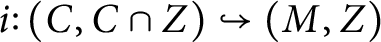 $i\colon (C,C\cap Z)\hookrightarrow (M,Z)$
of b-manifolds induces a canonical map
$i\colon (C,C\cap Z)\hookrightarrow (M,Z)$
of b-manifolds induces a canonical map
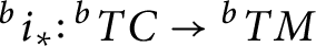 ${}^{b}i_{*}\colon {}^{b}TC\rightarrow {}^{b}TM$
that is injective by Lemma 1.5. This allows us to view
${}^{b}i_{*}\colon {}^{b}TC\rightarrow {}^{b}TM$
that is injective by Lemma 1.5. This allows us to view
 ${}^{b}TC$
as a Lie subalgebroid of
${}^{b}TC$
as a Lie subalgebroid of
 ${}^{b}TM$
. In particular, we have the following fact.
${}^{b}TM$
. In particular, we have the following fact.
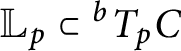
Lemma 1.8 If
 $C\subset (M,Z)$
is a b-submanifold, then
$C\subset (M,Z)$
is a b-submanifold, then
 $\mathbb {L}_{p}\subset {}^{b}T_{p}C$
for all
$\mathbb {L}_{p}\subset {}^{b}T_{p}C$
for all
 $p\in C\cap Z$
.
$p\in C\cap Z$
.
Proof Fixing some notation, we have anchor maps
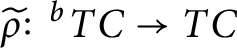 $\widetilde {\rho }\colon\; {}^{b}TC\rightarrow TC$
and
$\widetilde {\rho }\colon\; {}^{b}TC\rightarrow TC$
and
 $\rho \colon\; {}^{b}TM\rightarrow TM$
, and we put
$\rho \colon\; {}^{b}TM\rightarrow TM$
, and we put
 $\widetilde {\mathbb {L}}:=\text{Ker}(\widetilde {\rho }|_{C\cap Z})$
and
$\widetilde {\mathbb {L}}:=\text{Ker}(\widetilde {\rho }|_{C\cap Z})$
and
 $\mathbb {L}=\text{Ker}(\rho |_{Z})$
as before. If
$\mathbb {L}=\text{Ker}(\rho |_{Z})$
as before. If
 $i\colon (C,C\cap Z)\hookrightarrow (M,Z)$
denotes the inclusion, then we get a commutative diagram with exact rows, for points
$i\colon (C,C\cap Z)\hookrightarrow (M,Z)$
denotes the inclusion, then we get a commutative diagram with exact rows, for points
 $p\in C\cap Z$
:
$p\in C\cap Z$
:

We obtain
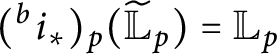 $({}^{b}i_{*})_{p}(\widetilde {\mathbb {L}}_{p})=\mathbb {L}_{p}$
: the inclusion “
$({}^{b}i_{*})_{p}(\widetilde {\mathbb {L}}_{p})=\mathbb {L}_{p}$
: the inclusion “
 $\subset $
” holds by the above diagram, and the equality follows by dimension reasons, since
$\subset $
” holds by the above diagram, and the equality follows by dimension reasons, since
 ${({}^{b}i_{*})_{p}} $
is injective. In particular,
${({}^{b}i_{*})_{p}} $
is injective. In particular,
 $\mathbb {L}_{p}$
is contained in the image of
$\mathbb {L}_{p}$
is contained in the image of
 ${({}^{b}i_{*})_{p}}$
, as we wanted to show.▪
${({}^{b}i_{*})_{p}}$
, as we wanted to show.▪
The notions of b-map and b-submanifold are compatible, as the next lemma shows.
Lemma 1.9 Let
 $f\colon (M_{1},Z_{1})\rightarrow (M_{2},Z_{2})$
be a b-map, and assume that we have b-submanifolds
$f\colon (M_{1},Z_{1})\rightarrow (M_{2},Z_{2})$
be a b-map, and assume that we have b-submanifolds
 $C_{1}\subset (M_{1},Z_{1})$
and
$C_{1}\subset (M_{1},Z_{1})$
and
 $C_{2}\subset (M_{2},Z_{2})$
such that
$C_{2}\subset (M_{2},Z_{2})$
such that
 $f(C_{1})\subset C_{2}$
.
$f(C_{1})\subset C_{2}$
.
-
(i) Restricting f gives a b-map
 $$ \begin{align*} f|_{C_{1}}:(C_{1},C_{1}\cap Z_{1})\longrightarrow (C_{2},C_{2}\cap Z_{2}).\end{align*} $$
-
(ii) Further,
$({}^{b}f_{*})|_{{}^{b}TC_1}={}^{b}(\,f|_{C_1})_{*}$
.

Proof
-
(i) We first note that
since f is a b-map and
$$ \begin{align*} (\,f|_{C_{1}})^{-1}(C_{2}\cap Z_{2})&=C_{1}\cap f^{-1}(C_{2}\cap Z_{2})=C_{1}\cap f^{-1}(C_{2})\cap f^{-1}(Z_{2})\\ &=C_{1}\cap f^{-1}(C_{2})\cap Z_{1}=C_{1}\cap Z_{1}, \end{align*} $$
$C_{1}\subset f^{-1}(C_{2})$
. Next, choosing
$p\in C_{1}\cap Z_{1}$
, we have to show that (1.4)We clearly have the inclusion “
$$ \begin{align} (\,f_{*})_{p}(T_{p}C_{1})+T_{f(p)}(C_{2}\cap Z_{2})=T_{f(p)}C_{2}. \end{align} $$
$\subset $
”. For the reverse, we choose
$v\in T_{f(p)}C_{2}$
. By transversality
$f\, \pitchfork\, Z_{2}$
, we know that
$(\,f_{*})_{p}(T_{p}M_{1})+ T_{f(p)}Z_{2}=T_{f(p)}M_{2}$
. So we have
$v=(\,f_{*})_{p}(x)+y$
for some
$x\in T_{p}M_{1}$
and
$y\in T_{f(p)}Z_{2}$
. Next, since
$C_{1}\, \pitchfork\, Z_{1}$
, we have
$T_{p}C_{1}+T_{p}Z_{1}=T_{p}M_{1}$
so that
$x=x_{1}+x_{2}$
for some
$x_{1}\in T_{p}C_{1}$
and
$x_{2}\in T_{p}Z_{1}$
. So we have (1.5)The term in square brackets clearly lies in
$$ \begin{align} v=(\,f_{*})_{p}(x_{1})+\big[(\,f_{*})_{p}(x_{2})+y\big]. \end{align} $$
$T_{f(p)}Z_{2}$
, and being equal to
$v-(\,f_{*})_{p}(x_{1})$
, it also lies in
$T_{f(p)}C_{2}$
. So it lies in
$T_{f(p)}(C_{2}\cap Z_{2})$
, using the transversality
$C_2\, \pitchfork\, Z_{2}$
. Hence, the decomposition (1.5) is as required in (1.4).
-
(ii) Denoting the inclusions
$i_{1}\colon\; (C_1,C_1\cap Z_{1})\hookrightarrow (M_{1},Z_{1})$
and
$i_{2}\colon\; (C_2,C_2\cap Z_{2})\hookrightarrow (M_{2},Z_{2})$
, we have
$f\circ i_{1}=i_{2}\circ f|_{C_1}$
. Hence by functoriality,
${}^{b}f_{*}\circ {}^{b}(i_{1})_{*}={}^{b}(i_{2})_{*}\circ {}^{b}(\,f|_{C_1})_{*}$
, which implies the claim.▪


1.3 Distributions on b-manifolds
We saw that the short exact sequence (1.1) does not split canonically. However, its restriction to suitable distributions does split.
Lemma 1.10 Let
 $(M,Z)$
be a b-manifold with anchor map
$(M,Z)$
be a b-manifold with anchor map
 $\rho \colon\; {}^{b}TM\rightarrow TM$
.
$\rho \colon\; {}^{b}TM\rightarrow TM$
.
-
(i) Given a distribution D on M that is tangent to Z, there exists a canonical splitting
$\sigma \colon\; D\rightarrow {}^{b}TM$
of the anchor
$\rho $
. -
(ii) Let
$\mathcal {D}$
denote the set of distributions on M tangent to Z, and let
$\mathcal {S}$
consist of the subbundles of
${}^{b}TM$
intersecting trivially
$\ker (\rho )$
. Then there is a bijection where the splitting
$$ \begin{align*} \mathcal{D}\longrightarrow\mathcal{S}\colon\; D\longmapsto\sigma(D), \end{align*} $$
$\sigma $
is as in (i). The inverse map reads
$D^{\prime }\mapsto \rho (D^{\prime })$
.


Proof
-
(i) One checks that the inclusion
$\Gamma (D)\subset \Gamma ({}^{b}TM)$
induces a well-defined vector bundle map where
$$ \begin{align*} \sigma\colon D\longrightarrow{}^{b}TM\colon\; v\longmapsto X_{p}, \end{align*} $$
$X\in \Gamma (D)$
is any extension of
$v\in D_{p}$
. This map
$\sigma $
satisfies
$\rho \circ \sigma = \text{Id} _{D}$
, so in particular
$\rho (\sigma (D))=D$
.
-
(ii) We only have to show that if
$D^{\prime }$
is a subbundle of
${}^{b}TM$
intersecting trivially
$\ker (\rho )$
, then
$\sigma (\rho (D^{\prime }))=D^{\prime }$
. Denote
$D:=\rho (D^{\prime })$
, a distribution on M tangent to Z. The canonical splitting
$\sigma \colon D\rightarrow {}^{b}TM$
is injective, and D and
$D^{\prime }$
have the same rank, hence it suffices to show that
$\sigma (D)\subset D^{\prime }$
. If X is a section of D, then
$X=\rho (Y)$
for unique
$Y\in \Gamma (D^{\prime })$
. We get and since the anchor
$$ \begin{align*} \rho\big(\sigma(X)\big)=X=\rho(Y), \end{align*} $$
$\rho $
is injective on sections, this implies that
$\sigma (X)=Y$
.▪


Corollary 1.11 Let
 $f\colon (M_{1},Z_{1})\rightarrow (M_{2},Z_{2})$
be a b-map of constant rank. Notice that
$f\colon (M_{1},Z_{1})\rightarrow (M_{2},Z_{2})$
be a b-map of constant rank. Notice that
 $\text{Ker}(\,f_{*})$
is a distribution on
$\text{Ker}(\,f_{*})$
is a distribution on
 $M_{1}$
that is tangent to
$M_{1}$
that is tangent to
 $Z_{1}$
. It satisfies
$Z_{1}$
. It satisfies
 $$ \begin{align*} \sigma\big(\text{Ker}(\,f_{*})\big)= \text{Ker}({}^{b}f_{*}), \end{align*} $$
where
 $\sigma \colon \text{Ker}(\,f_{*})\rightarrow {}^{b}TM_{1}$
denotes the canonical splitting of the anchor
$\sigma \colon \text{Ker}(\,f_{*})\rightarrow {}^{b}TM_{1}$
denotes the canonical splitting of the anchor
 $\rho _{1}$
.
$\rho _{1}$
.

1.4 Vector Bundles in the b-category
If
 $(M,Z)$
is a b-manifold and
$(M,Z)$
is a b-manifold and
 $\pi \colon E\rightarrow M$
a vector bundle, then
$\pi \colon E\rightarrow M$
a vector bundle, then
 $(E,E|_{Z})$
is naturally a b-manifold and the projection
$(E,E|_{Z})$
is naturally a b-manifold and the projection
 $\pi \colon (E,E|_{Z})\rightarrow (M,Z)$
is a b-map. Along the zero section
$\pi \colon (E,E|_{Z})\rightarrow (M,Z)$
is a b-map. Along the zero section
 $M\subset E$
, the b-tangent bundle
$M\subset E$
, the b-tangent bundle
 ${}^{b}TE$
splits canonically as follows.
${}^{b}TE$
splits canonically as follows.
Lemma 1.12 Let
 $(M,Z)$
be a b-manifold and let
$(M,Z)$
be a b-manifold and let
 $\pi \colon E\rightarrow M$
be a vector bundle. Then at points
$\pi \colon E\rightarrow M$
be a vector bundle. Then at points
 $p\in M$
, we have a canonical decomposition
$p\in M$
, we have a canonical decomposition
 $$ \begin{align*} {}^{b}T_{p}E\cong{}^{b}T_{p}M\oplus E_{p}. \end{align*} $$
Proof Denote by
 $VE:=\text{Ker}(\pi _{*})$
the vertical bundle. By Corollary 1.11 there is a canonical lift
$VE:=\text{Ker}(\pi _{*})$
the vertical bundle. By Corollary 1.11 there is a canonical lift
 $\sigma \colon VE\hookrightarrow {}^{b}TE$
such that
$\sigma \colon VE\hookrightarrow {}^{b}TE$
such that
 $\sigma (VE)=\text{Ker}({}^{b}\pi _{*})$
. So we get a short exact sequence of vector bundles over E:
$\sigma (VE)=\text{Ker}({}^{b}\pi _{*})$
. So we get a short exact sequence of vector bundles over E:

Here,
 $$\begin{align*}\pi^{*}({}^{b}TM)=\big\{(e,v)\in E\times{}^{b}TM:\pi(e)=pr(v)\big\} \end{align*}$$
is the pullback of the vector bundle
 $pr\colon {}^{b}TM\rightarrow M$
by
$pr\colon {}^{b}TM\rightarrow M$
by
 $\pi $
, and the surjective vector bundle map
$\pi $
, and the surjective vector bundle map
 $$ \begin{align*} \widetilde{{}^{b}\pi_{*}}\colon {}^{b}TE\longrightarrow \pi^{*}({}^{b}TM),\quad(e,v)\longmapsto \left[e,({}^{b}\pi_{*})_{e}(v)\right] \end{align*} $$
is induced by the b-map
 $\pi \colon (E,E|_{Z})\rightarrow (M,Z)$
.
$\pi \colon (E,E|_{Z})\rightarrow (M,Z)$
.
Restricting (1.6) to the zero section
 $M\subset E$
gives a short exact sequence of vector bundles over M:
$M\subset E$
gives a short exact sequence of vector bundles over M:
 $$ \begin{align*} 0\longrightarrow E \hookrightarrow{}^{b}TE|_{M}\overset{{{}^{b}\pi_{*}}}{\longrightarrow}{}^{b}TM\longrightarrow 0. \end{align*} $$
This sequence splits canonically through the map
 ${}^{b}i_{*}\colon {}^{b}TM\rightarrow {}^{b}TE|_{M}$
induced by the inclusion
${}^{b}i_{*}\colon {}^{b}TM\rightarrow {}^{b}TE|_{M}$
induced by the inclusion
 $i\colon (M,Z)\hookrightarrow (E,E|_{Z})$
.▪
$i\colon (M,Z)\hookrightarrow (E,E|_{Z})$
.▪
The following result makes use of the decomposition introduced in Lemma 1.12.
Lemma 1.13
-
(i) Let
$\pi \colon (E,E|_{Z})\rightarrow (M,Z)$
be a vector bundle over the b-manifold
$(M,Z)$
. Denote by
$\rho $
and
$\widetilde {\rho }$
the anchor maps of
${}^{b}TM$
and
${}^{b}TE$
respectively. Under the decomposition of Lemma 1.12, we have that the map equals
$$ \begin{align*} \widetilde{\rho}|_{M}\colon {}^{b}TE|_{M}\cong{}^{b}TM\oplus E\longrightarrow TE|_{M}\cong TM\oplus E \end{align*} $$
$\rho \oplus {Id} _{E}$
.
-
(ii) Consider a morphism
$\varphi $
of vector bundles over b-manifolds covering a b-map f:(1.7)Then
$\varphi $
is a b-map, and its b-derivative along the zero section equals
$$ \begin{align*} {}^{b}\varphi_{*}|_M\colon {}^{b}TE_{1}|_M\cong{}^{b}TM_{1}\oplus E_{1}\to {}^{b}TE_{2}|_M\cong{}^{b}TM_{2}\oplus E_{2} \end{align*} $$
${}^{b}f_{*}\oplus \varphi $
.


Proof
-
(i) Since M is a b-submanifold of
$(E,E|_{Z})$
, we have that
${}^{b}TM$
is a Lie subalgebroid of
${}^{b}TE$
. In particular,
$\widetilde {\rho }$
and
$\rho $
agree on
${}^{b}TM$
. Next, we know that
$\widetilde {\rho }$
takes
$E\subset {}^{b}TE|_{M}$
isomorphically to
$E\subset TE|_{M}$
, thanks to Lemma 1.5 applied to
$\pi $
. To see that
$\widetilde {\rho }|_{E}= \text{Id} _{E}$
, we choose
$v\in E_{p}$
and extend it to
$V\in \Gamma (VE)$
. Denote by
$\sigma \colon VE\hookrightarrow {}^{b}TE$
the canonical splitting of
$\widetilde {\rho }$
, as in the proof of Lemma 1.12. Then
$\widetilde {\rho }(v)=[\widetilde {\rho }(\sigma (V))]_{p}=V_{p}=v$
. -
(ii) It is routine to check that
$\varphi $
is a b-map, so we only prove the second statement. Taking the b-derivative of both sides of the equality
$\pi _2\circ \varphi =f\circ \pi _1$
at a point
$p\in M_{1}$
, we know that
$({}^{b}\pi _{2})_{*}({}^{b}\varphi _{*}(E_{1})_{p})={}^{b}f_{*}(({}^{b}\pi _{1})_{*}(E_{1})_{p})=0$
, since
$(E_{1})_{p}=\text{Ker}[({}^{b}\pi _{1})_{*}]_{p}$
. Hence,
${}^{b}\varphi _{*}(E_{1})_{p}\subset \text{Ker}[({}^{b}\pi _{2})_{*}]_{f(p)}=(E_{2})_{f(p)}$
by the proof of Lemma 1.12. Using (i) and the diagram (1.2), we have a commutative diagram(1.8)It implies that
Finally,
$$ \begin{align*} {}^{b}\varphi_{*}|_{(E_{1})_{p}}= \varphi_{*}|_{(E_{1})_{p}}= \varphi|_{(E_{1})_{p}}. \end{align*} $$
$ {}^{b}\varphi _{*}|_{{}^{b}TM_{1}}={}^{b}f_{*}$
holds by Lemma 1.9(ii).▪


1.5 Log-symplectic and b-symplectic Structures
The b-geometry formalism can be used to describe a certain class of Poisson structures, called log-symplectic structures. These can indeed be regarded as symplectic structures on the b-tangent bundle.
Definition 1.14 A Poisson structure on a manifold M is a bivector field
 $\Pi \in \Gamma (\wedge ^{2}TM)$
such that the bracket
$\Pi \in \Gamma (\wedge ^{2}TM)$
such that the bracket
 $\{\,f,g\}=\Pi (df,dg)$
is a Lie bracket on
$\{\,f,g\}=\Pi (df,dg)$
is a Lie bracket on
 $C^{\infty }(M)$
. Equivalently, the bivector field
$C^{\infty }(M)$
. Equivalently, the bivector field
 $\Pi $
must satisfy
$\Pi $
must satisfy
 $[\Pi ,\Pi ]=0$
, where
$[\Pi ,\Pi ]=0$
, where
 $[\cdot ,\cdot ]$
is the Schouten–Nijenhuis bracket of multivector fields. A smooth map
$[\cdot ,\cdot ]$
is the Schouten–Nijenhuis bracket of multivector fields. A smooth map
 $f\colon (M_{1},\Pi _{1})\rightarrow (M_{2},\Pi _{2})$
is a Poisson map if the pullback
$f\colon (M_{1},\Pi _{1})\rightarrow (M_{2},\Pi _{2})$
is a Poisson map if the pullback
 $f^{*}\colon (C^{\infty }(M_{2}),\{\cdot ,\cdot \}_{2})\rightarrow (C^{\infty }(M_{1}),\{\cdot ,\cdot \}_{1})$
is a Lie algebra homomorphism.
$f^{*}\colon (C^{\infty }(M_{2}),\{\cdot ,\cdot \}_{2})\rightarrow (C^{\infty }(M_{1}),\{\cdot ,\cdot \}_{1})$
is a Lie algebra homomorphism.
The bivector
 $\Pi $
induces a bundle map
$\Pi $
induces a bundle map
 $\Pi ^{\sharp }\colon T^{*}M\rightarrow TM$
by
$\Pi ^{\sharp }\colon T^{*}M\rightarrow TM$
by
 $$ \begin{align*} \big\langle \Pi_{p}^{\sharp}(\alpha),\beta\big\rangle=\Pi_{p}(\alpha,\beta)\forall\alpha,\beta\in T_{p}^{*}M, \end{align*} $$
and the rank of
 $\Pi $
at
$\Pi $
at
 $p\in M$
is defined to be the rank of the linear map
$p\in M$
is defined to be the rank of the linear map
 $\Pi ^{\sharp }_{p}$
. Poisson structures of full rank correspond with symplectic structures via
$\Pi ^{\sharp }_{p}$
. Poisson structures of full rank correspond with symplectic structures via
 $\omega \leftrightarrow -\Pi ^{-1}$
.
$\omega \leftrightarrow -\Pi ^{-1}$
.
For every
 $f\in C^{\infty }(M)$
, the operator
$f\in C^{\infty }(M)$
, the operator
 $\{\,f,\cdot \}$
is a derivation of
$\{\,f,\cdot \}$
is a derivation of
 $C^{\infty }(M)$
. The corresponding vector field
$C^{\infty }(M)$
. The corresponding vector field
 $X_{f}=\Pi ^{\sharp }(df)$
is the Hamiltonian vector field of f. Any Poisson manifold
$X_{f}=\Pi ^{\sharp }(df)$
is the Hamiltonian vector field of f. Any Poisson manifold
 $(M,\Pi )$
comes with a (singular) distribution
$(M,\Pi )$
comes with a (singular) distribution
 $Im (\Pi ^{\sharp })$
, generated by the Hamiltonian vector fields. This distribution is integrable (in the sense of Stefan–Sussman), and each leaf
$Im (\Pi ^{\sharp })$
, generated by the Hamiltonian vector fields. This distribution is integrable (in the sense of Stefan–Sussman), and each leaf
 $\mathcal {O}$
of the associated foliation has an induced symplectic structure
$\mathcal {O}$
of the associated foliation has an induced symplectic structure
 $\omega _{\mathcal {O}}:=-(\Pi |_{\mathcal {O}})^{-1}$
.
$\omega _{\mathcal {O}}:=-(\Pi |_{\mathcal {O}})^{-1}$
.
Definition 1.15 A Poisson structure
 $\Pi $
on a manifold
$\Pi $
on a manifold
 $M^{2n}$
is called log-symplectic if
$M^{2n}$
is called log-symplectic if
 $\wedge ^{n}\Pi $
is transverse to the zero section of the line bundle
$\wedge ^{n}\Pi $
is transverse to the zero section of the line bundle
 $\wedge ^{2n}TM$
.
$\wedge ^{2n}TM$
.
Note that a log-symplectic structure
 $\Pi $
is of full rank everywhere, except at points lying in the set
$\Pi $
is of full rank everywhere, except at points lying in the set
 $Z:=(\wedge ^{n}\Pi )^{-1}(0)$
, called the singular locus of
$Z:=(\wedge ^{n}\Pi )^{-1}(0)$
, called the singular locus of
 $\Pi $
. If Z is nonempty, then it is a smooth hypersurface by the transversality condition, and we call
$\Pi $
. If Z is nonempty, then it is a smooth hypersurface by the transversality condition, and we call
 $\Pi $
bona fide log-symplectic. In that case, Z is a Poisson submanifold of
$\Pi $
bona fide log-symplectic. In that case, Z is a Poisson submanifold of
 $(M,\Pi )$
with an induced Poisson structure that is regular of corank-one. If Z is empty, then
$(M,\Pi )$
with an induced Poisson structure that is regular of corank-one. If Z is empty, then
 $\Pi $
defines a symplectic structure on M.
$\Pi $
defines a symplectic structure on M.
Since log-symplectic structures come with a specified hypersurface, it seems plausible that they have a b-geometric interpretation. As it turns out, log-symplectic structures are exactly the symplectic structures of the b-category.
Definition 1.16 A
b-symplectic form on a b-manifold
 $(M^{2n},Z)$
is a
$(M^{2n},Z)$
is a
 ${}^{b}d$
-closed and non-degenerate b-two-form
${}^{b}d$
-closed and non-degenerate b-two-form
 $\omega \in {}^{b}\Omega ^{2}(M)$
.
$\omega \in {}^{b}\Omega ^{2}(M)$
.
Here, non-degeneracy means that the bundle map
 $\omega ^{\flat }\colon\; {}^{b}TM\rightarrow {}^{b}T^{*}M$
is an isomorphism, or equivalently that
$\omega ^{\flat }\colon\; {}^{b}TM\rightarrow {}^{b}T^{*}M$
is an isomorphism, or equivalently that
 $\wedge ^{n}\omega $
is a nowhere vanishing element of
$\wedge ^{n}\omega $
is a nowhere vanishing element of
 ${}^{b}\Omega ^{2n}(M)$
.
${}^{b}\Omega ^{2n}(M)$
.
Example 1.17 [Reference Guillemin, Miranda and Pires11, Example 9] In analogy with the symplectic case, the b-cotangent bundle
 ${}^{b}T^{*}M$
of a b-manifold
${}^{b}T^{*}M$
of a b-manifold
 $(M,Z)$
is b-symplectic in a canonical way. Note that
$(M,Z)$
is b-symplectic in a canonical way. Note that
 $({}^{b}T^{*}M,{}^{b}T^{*}M|_{Z})$
is naturally a b-manifold, and that the bundle projection
$({}^{b}T^{*}M,{}^{b}T^{*}M|_{Z})$
is naturally a b-manifold, and that the bundle projection
 $\pi \colon ({}^{b}T^{*}M,{}^{b}T^{*}M|_{Z})\rightarrow (M,Z)$
is a b-map. The tautological b-one-form
$\pi \colon ({}^{b}T^{*}M,{}^{b}T^{*}M|_{Z})\rightarrow (M,Z)$
is a b-map. The tautological b-one-form
 $\theta \in {}^{b}\Omega ^{1}({}^{b}T^{*}M)$
is defined by
$\theta \in {}^{b}\Omega ^{1}({}^{b}T^{*}M)$
is defined by
 $$ \begin{align*} \theta_{\xi}(v)=\langle \xi,({}^{b}\pi_{*})_{\xi}(v)\rangle, \end{align*} $$
where
 $\xi \in {}^{b}T^{*}_{\pi (\xi )}M$
and
$\xi \in {}^{b}T^{*}_{\pi (\xi )}M$
and
 $v\in {}^{b}T_{\xi }({}^{b}T^{*}M)$
. Its differential
$v\in {}^{b}T_{\xi }({}^{b}T^{*}M)$
. Its differential
 $-{}^{b}d\theta $
is a b-symplectic form on
$-{}^{b}d\theta $
is a b-symplectic form on
 ${}^{b}T^{*}M$
. To see this, choose coordinates
${}^{b}T^{*}M$
. To see this, choose coordinates
 $(x_{1},\dots ,x_{n})$
on M adapted to
$(x_{1},\dots ,x_{n})$
on M adapted to
 $Z=\{x_{1}=0\}$
, and let
$Z=\{x_{1}=0\}$
, and let
 $(y_{1},\dots ,y_{n})$
denote the fiber coordinates on
$(y_{1},\dots ,y_{n})$
denote the fiber coordinates on
 ${}^{b}T^{*}M$
with respect to the local frame
${}^{b}T^{*}M$
with respect to the local frame
 $\{\frac {dx_{1}}{x_{1}},dx_{2},\dots ,dx_{n}\}$
. The tautological b-one form is then given by
$\{\frac {dx_{1}}{x_{1}},dx_{2},\dots ,dx_{n}\}$
. The tautological b-one form is then given by
 $$ \begin{align*} \theta=y_{1}\frac{dx_{1}}{x_{1}}+\sum_{i=2}^{n}y_{i}dx_{i}, \end{align*} $$
with exterior derivative
 $$ \begin{align*} -{}^{b}d\theta=\frac{dx_{1}}{x_{1}}\wedge dy_{1}+\sum_{i=2}^{n}dx_{i}\wedge dy_{i}. \end{align*} $$
A log-symplectic structure on M with singular locus Z is nothing but a b-symplectic structure on the b-manifold
 $(M,Z)$
; see [Reference Guillemin, Miranda and Pires11, Proposition 20]. Indeed, given a b-symplectic form
$(M,Z)$
; see [Reference Guillemin, Miranda and Pires11, Proposition 20]. Indeed, given a b-symplectic form
 $\omega $
on
$\omega $
on
 $(M,Z)$
, its negative inverse
$(M,Z)$
, its negative inverse
 ${}^{b}\Pi ^{\sharp }:={-}(\omega ^{\flat })^{-1}\colon {}^{b}T^{*}M\rightarrow {}^{b}TM$
defines a b-bivector field
${}^{b}\Pi ^{\sharp }:={-}(\omega ^{\flat })^{-1}\colon {}^{b}T^{*}M\rightarrow {}^{b}TM$
defines a b-bivector field
 ${}^{b}\Pi \in \Gamma (\wedge ^{2}({}^{b}TM))$
, and applying the anchor map
${}^{b}\Pi \in \Gamma (\wedge ^{2}({}^{b}TM))$
, and applying the anchor map
 $\rho $
to it yields a bivector field
$\rho $
to it yields a bivector field
 $\Pi :=\rho ({}^{b}\Pi )\in \Gamma (\wedge ^{2}TM)$
that is log-symplectic with singular locus Z. Conversely, a log-symplectic structure
$\Pi :=\rho ({}^{b}\Pi )\in \Gamma (\wedge ^{2}TM)$
that is log-symplectic with singular locus Z. Conversely, a log-symplectic structure
 $\Pi $
on M with singular locus Z lifts uniquely under
$\Pi $
on M with singular locus Z lifts uniquely under
 $\rho $
to a non-degenerate b-bivector field
$\rho $
to a non-degenerate b-bivector field
 ${}^{b}\Pi $
, whose negative inverse is a b-symplectic form on
${}^{b}\Pi $
, whose negative inverse is a b-symplectic form on
 $(M,Z)$
. These processes are summarized in the following diagram:
$(M,Z)$
. These processes are summarized in the following diagram:

We will switch between the b-symplectic and the log-symplectic (i.e., Poisson) viewpoint, depending on which one is the most convenient.
1.6 A Relative b-Moser Theorem
We will need a relative Moser theorem in the b-symplectic setting. First, we prove the following b-geometric version of the relative Poincaré lemma [Reference Cannas da Silva3, Proposition 6.8].
Lemma 1.18 Let
 $(M,Z)$
be a b-manifold and let
$(M,Z)$
be a b-manifold and let
 $C\subset (M,Z)$
be a b-submanifold. Denote the inclusion by
$C\subset (M,Z)$
be a b-submanifold. Denote the inclusion by
 $i\colon (C,C\cap Z)\hookrightarrow (M,Z)$
. If
$i\colon (C,C\cap Z)\hookrightarrow (M,Z)$
. If
 $\beta \in {}^{b}\Omega ^{k}(M)$
is
$\beta \in {}^{b}\Omega ^{k}(M)$
is
 ${}^{b}d$
-closed and
${}^{b}d$
-closed and
 ${}^{b}i^{*}\beta =0$
, then there exist a neighborhood U of C and
${}^{b}i^{*}\beta =0$
, then there exist a neighborhood U of C and
 $\eta \in {}^{b}\Omega ^{k-1}(U)$
such that
$\eta \in {}^{b}\Omega ^{k-1}(U)$
such that
 $$ \begin{align*} \left\{\!\!\!\!\begin{array}{l} ^{b}d\eta=\beta|_{U},\\ \eta|_{C}=0 \end{array}\right. \end{align*} $$
Proof We adapt the proof of [Reference Cannas da Silva3, Proposition 6.8]. We first choose a suitable tubular neighborhood of C that is compatible with the hypersurface Z. Due to transversality
 $C\, \pitchfork\, Z$
, we can pick a complement V to
$C\, \pitchfork\, Z$
, we can pick a complement V to
 $TC$
in
$TC$
in
 $TM|_{C}$
such that
$TM|_{C}$
such that
 $V_{p}\subset T_{p}Z$
for all
$V_{p}\subset T_{p}Z$
for all
 $p\in C\cap Z$
. Fix a Riemannian metric g for which
$p\in C\cap Z$
. Fix a Riemannian metric g for which
 $Z\subset (M,g)$
is totally geodesic (e.g.,[Reference Milnor19, Lemma 6.8]). The associated exponential map then establishes a b-diffeomorphism between a neighborhood of C in
$Z\subset (M,g)$
is totally geodesic (e.g.,[Reference Milnor19, Lemma 6.8]). The associated exponential map then establishes a b-diffeomorphism between a neighborhood of C in
 $(V,V|_{C\cap Z})$
and a neighborhood of C in
$(V,V|_{C\cap Z})$
and a neighborhood of C in
 $(M,Z)$
.
$(M,Z)$
.
So we can work instead on the total space of
 $\pi \colon (V,V|_{C\cap Z})\rightarrow (C,C\cap Z)$
. Consider the retraction of V onto C given by
$\pi \colon (V,V|_{C\cap Z})\rightarrow (C,C\cap Z)$
. Consider the retraction of V onto C given by
 ${r}\colon V\times [0,1]\rightarrow V\colon (p,v,t)\mapsto (p,tv)$
, and notice that the
${r}\colon V\times [0,1]\rightarrow V\colon (p,v,t)\mapsto (p,tv)$
, and notice that the
 ${r}_{t}$
are b-maps. The associated time-dependent vector field
${r}_{t}$
are b-maps. The associated time-dependent vector field
 $X_{t}$
is given by
$X_{t}$
is given by
 $X_{t}(p,v)={\frac {1}{t}v}$
, which is a b-vector field that vanishes along C. It follows that we get a well-defined b-de Rham homotopy operator
$X_{t}(p,v)={\frac {1}{t}v}$
, which is a b-vector field that vanishes along C. It follows that we get a well-defined b-de Rham homotopy operator
 $$ \begin{align*} I\colon {}^{b}\Omega^{k}(V)\longrightarrow{}^{b}\Omega^{k-1}(V)\colon \alpha\longmapsto\int_{0}^{1}{}^{b}{r}_{t}^{*}(\iota_{X_{t}}\alpha)dt, \end{align*} $$
which satisfies
 $$ \begin{align} {}^{b}{r}_{1}^{*}\alpha-{}^{b}{r}_{0}^{*}\alpha={}^{b}d I(\alpha)+I({}^{b}d\alpha). \end{align} $$
Since
 ${r}_{1}= \text{Id} $
and
${r}_{1}= \text{Id} $
and
 ${r}_{0}=i\circ \pi $
, formula (1.10) gives
${r}_{0}=i\circ \pi $
, formula (1.10) gives
 $\beta ={}^{b}d I(\beta )$
. Now set
$\beta ={}^{b}d I(\beta )$
. Now set
 $\eta :=I(\beta )$
.▪
$\eta :=I(\beta )$
.▪
Proposition 1.19 (Relative b-Moser Theorem)
Let
 $(M,Z)$
be a b-manifold and let
$(M,Z)$
be a b-manifold and let
 $C\subset (M,Z)$
be a b-submanifold. If
$C\subset (M,Z)$
be a b-submanifold. If
 $\omega _{0}$
and
$\omega _{0}$
and
 $\omega _{1}$
are b-symplectic forms on
$\omega _{1}$
are b-symplectic forms on
 $(M,Z)$
such that
$(M,Z)$
such that
 $\omega _{0}|_{C}=\omega _{1}|_{C}$
, then there exists a b-diffeomorphism
$\omega _{0}|_{C}=\omega _{1}|_{C}$
, then there exists a b-diffeomorphism
 $\varphi $
between neighborhoods of C such that
$\varphi $
between neighborhoods of C such that
 $\varphi |_{C}= \text{Id} $
and
$\varphi |_{C}= \text{Id} $
and
 ${}^{b}\varphi ^{*}\omega _{1}=\omega _{0}$
.
${}^{b}\varphi ^{*}\omega _{1}=\omega _{0}$
.
Proof Consider the convex combination
 $\omega _{t}:=\omega _{0}+t(\omega _{1}-\omega _{0})$
for
$\omega _{t}:=\omega _{0}+t(\omega _{1}-\omega _{0})$
for
 $t\in [0,1]$
. There exists a neighborhood U of C such that
$t\in [0,1]$
. There exists a neighborhood U of C such that
 $\omega _{t}$
is non-degenerate on U for all
$\omega _{t}$
is non-degenerate on U for all
 $t\in [0,1]$
. Shrinking U if necessary, Lemma 1.18 yields
$t\in [0,1]$
. Shrinking U if necessary, Lemma 1.18 yields
 $\eta \in {}^{b}\Omega ^{1}(U)$
such that
$\eta \in {}^{b}\Omega ^{1}(U)$
such that
 $\omega _{1}-\omega _{0}={}^{b}d\eta $
and
$\omega _{1}-\omega _{0}={}^{b}d\eta $
and
 $\eta |_{C}=0$
. As in the usual Moser trick, it now suffices to solve the equation
$\eta |_{C}=0$
. As in the usual Moser trick, it now suffices to solve the equation
 $$ \begin{align*} \iota_{X_{t}}\omega_{t}+\eta=0 \end{align*} $$
for
 $X_{t}\in {}^{b}\mathfrak {X}(U)$
, which is possible by non-degeneracy of
$X_{t}\in {}^{b}\mathfrak {X}(U)$
, which is possible by non-degeneracy of
 $\omega _{t}$
. The b-vector fields
$\omega _{t}$
. The b-vector fields
 $X_{t}$
thus obtained vanish along C, since
$X_{t}$
thus obtained vanish along C, since
 $\eta |_{C}=0$
. Further shrinking U if necessary, we can integrate the
$\eta |_{C}=0$
. Further shrinking U if necessary, we can integrate the
 $X_{t}$
to an isotopy
$X_{t}$
to an isotopy
 $\{{\phi _{t}}\}_{t\in [0,1]}$
defined on U. Note that the
$\{{\phi _{t}}\}_{t\in [0,1]}$
defined on U. Note that the
 ${\phi _{t}}$
are b-diffeomorphisms that restrict to the identity on C. By the usual Moser argument, we have
${\phi _{t}}$
are b-diffeomorphisms that restrict to the identity on C. By the usual Moser argument, we have
 ${}^{b}{\phi _{1}}^{*}\omega _{1}=\omega _{0}$
, so setting
${}^{b}{\phi _{1}}^{*}\omega _{1}=\omega _{0}$
, so setting
 $\varphi :={\phi _{1}}$
finishes the proof.▪
$\varphi :={\phi _{1}}$
finishes the proof.▪
Remark 1.20 We learnt from Ralph Klaasse that the work in progress [Reference Klaasse and Lanius15] contains a version of Proposition 1.19 that holds in the more general setting of symplectic Lie algebroids.
2 b-coisotropic Submanifolds and the b-Gotay Theorem
This section is devoted to coisotropic submanifolds of b-symplectic manifolds that are transverse to the degeneracy hypersurface. The main result is Theorem 2.13, a b-symplectic version of Gotay’s theorem, which implies a normal form statement around such submanifolds. This can be used, for instance, to study the deformation theory of b-coisotropic submanifolds [Reference Geudens and Zambon7].
2.1 b-coisotropic Submanifolds
In this subsection, we introduce b-coisotropic submanifolds and discuss some of their main features. First, recall the definition of a coisotropic submanifold in Poisson geometry.
Definition 2.1 Let
 $(M,\Pi )$
be a Poisson manifold with associated Poisson bracket
$(M,\Pi )$
be a Poisson manifold with associated Poisson bracket
 $\{\cdot ,\cdot \}$
. A submanifold
$\{\cdot ,\cdot \}$
. A submanifold
 $C\subset M$
is coisotropic if the following equivalent conditions hold:
$C\subset M$
is coisotropic if the following equivalent conditions hold:
-
(i)
$\Pi ^{\sharp }(TC^{0})\subset TC$
, where
$TC^{0}\subset T^{*}M|_{C}$
denotes the annihilator of
$TC$
. -
(ii)
$\{\mathcal {I}_{C},\mathcal {I}_{C}\}\subset \mathcal {I}_{C}$
, where
$\mathcal {I}_{C}:=\{\,f\in C^{\infty }(M): f|_{C}=0\}$
denotes the vanishing ideal of C. -
(iii)
$T_{p}C\cap T_{p}\mathcal {O}$
is a coisotropic subspace of the symplectic vector space
$(T_{p}\mathcal {O},-(\Pi |_{\mathcal {O}})^{-1}_{p})$
for all
$p\in C$
, where
$\mathcal {O}$
denotes the symplectic leaf through p.


The singular distribution
 $\Pi ^{\sharp }(TC^{0})$
on C appearing above is called the characteristic distribution. If
$\Pi ^{\sharp }(TC^{0})$
on C appearing above is called the characteristic distribution. If
 $\Pi ={-}\omega ^{-1}$
is symplectic, the coisotropicity condition becomes
$\Pi ={-}\omega ^{-1}$
is symplectic, the coisotropicity condition becomes
 $TC^{\omega }\subset TC$
.
$TC^{\omega }\subset TC$
.
Definition 2.2 Let
 $(M,Z,\omega )$
be a b-symplectic manifold, and denote by
$(M,Z,\omega )$
be a b-symplectic manifold, and denote by
 $\Pi $
the corresponding Poisson bivector field on M. A submanifold C of M is called
b-coisotropic if it is coisotropic with respect to
$\Pi $
the corresponding Poisson bivector field on M. A submanifold C of M is called
b-coisotropic if it is coisotropic with respect to
 $\Pi $
and a b-submanifold (i.e., transverse to Z).
$\Pi $
and a b-submanifold (i.e., transverse to Z).
Remark 2.3 A b-coisotropic submanifold
 $C^{n}\subset (M^{2n},Z,\Pi )$
of middle dimension is necessarily Lagrangian; i.e.,
$C^{n}\subset (M^{2n},Z,\Pi )$
of middle dimension is necessarily Lagrangian; i.e.,
 $T_{p}C\cap T_{p}\mathcal {O}$
is a Lagrangian subspace of the symplectic vector space
$T_{p}C\cap T_{p}\mathcal {O}$
is a Lagrangian subspace of the symplectic vector space
 $(T_{p}\mathcal {O},-(\Pi |_{\mathcal {O}})^{-1}_{p})$
for all
$(T_{p}\mathcal {O},-(\Pi |_{\mathcal {O}})^{-1}_{p})$
for all
 $p\in C$
, where
$p\in C$
, where
 $\mathcal {O}$
denotes the symplectic leaf through p. Indeed, at points away from Z there is nothing to prove. At points
$\mathcal {O}$
denotes the symplectic leaf through p. Indeed, at points away from Z there is nothing to prove. At points
 $p\in C\cap Z$
, we have
$p\in C\cap Z$
, we have
 $$ \begin{align*} \dim(T_{p}C\cap T_{p}\mathcal{O})\leq \dim(T_{p}C\cap T_{p}Z)=n-1, \end{align*} $$
where the last equality follows from transversality
 $C\, \pitchfork\, Z$
. On the other hand,
$C\, \pitchfork\, Z$
. On the other hand,
 $T_{p}C\cap T_{p}\mathcal {O}$
is at least
$T_{p}C\cap T_{p}\mathcal {O}$
is at least
 $(n-1)$
-dimensional, being a coisotropic subspace of the
$(n-1)$
-dimensional, being a coisotropic subspace of the
 $(2n-2)$
-dimensional symplectic vector space
$(2n-2)$
-dimensional symplectic vector space
 $T_{p}\mathcal {O}$
. Hence,
$T_{p}\mathcal {O}$
. Hence,
 $\dim (T_{p}C\cap T_{p}\mathcal {O})=n-1$
, which proves the claim.
$\dim (T_{p}C\cap T_{p}\mathcal {O})=n-1$
, which proves the claim.
Definition 2.2 can be rephrased in terms of the b-symplectic form
 $\omega $
: a b-coisotropic submanifold is precisely a b-submanifold C such that
$\omega $
: a b-coisotropic submanifold is precisely a b-submanifold C such that
 $({}^{b}TC)^\omega \subset {}^{b}TC$
.
$({}^{b}TC)^\omega \subset {}^{b}TC$
.
Proposition 2.4 Let C be a b-submanifold of a b-symplectic manifold
 $(M,Z,\omega )$
. Then C is coisotropic if and only if
$(M,Z,\omega )$
. Then C is coisotropic if and only if
 $({}^{b}TC)^\omega \subset {}^{b}TC$
.
$({}^{b}TC)^\omega \subset {}^{b}TC$
.
Notice that the latter condition states that
 ${}^bTC$
is a coisotropic subbundle of the symplectic vector bundle
${}^bTC$
is a coisotropic subbundle of the symplectic vector bundle
 $(^bTM|_C, \omega |_{C})$
.
$(^bTM|_C, \omega |_{C})$
.
Proof If C is coisotropic, then at points of
 $C \cap (M\setminus Z)$
, we have that
$C \cap (M\setminus Z)$
, we have that
 $TC^\omega \subset TC$
, i.e.,
$TC^\omega \subset TC$
, i.e.,
 $({}^{b}TC)^\omega \subset {}^{b}TC$
. By continuity, this inclusion of subbundles holds at all points of C. Conversely, if this inclusion holds on C, it follows that
$({}^{b}TC)^\omega \subset {}^{b}TC$
. By continuity, this inclusion of subbundles holds at all points of C. Conversely, if this inclusion holds on C, it follows that
 $C \cap (M\setminus Z)$
is coisotropic in
$C \cap (M\setminus Z)$
is coisotropic in
 $M\setminus Z$
, and using characterization (ii) in Definition 2.1, we see that C is coisotropic in M.▪
$M\setminus Z$
, and using characterization (ii) in Definition 2.1, we see that C is coisotropic in M.▪
We give an alternative description of the characteristic distribution of a b-coisotropic submanifold.
Lemma 2.5 Let C be any b-submanifold of a b-symplectic manifold
 $(M,Z,\omega )$
, and let
$(M,Z,\omega )$
, and let
 $\rho \colon {}^{b}TM\rightarrow TM$
denote the anchor of
$\rho \colon {}^{b}TM\rightarrow TM$
denote the anchor of
 ${}^{b}TM$
so that
${}^{b}TM$
so that
 $\Pi =\rho ({-}\omega ^{-1})$
is the Poisson bivector corresponding with
$\Pi =\rho ({-}\omega ^{-1})$
is the Poisson bivector corresponding with
 $\omega $
. Then
$\omega $
. Then
 $$ \begin{align} \rho\big(({}^{b}TC)^{\omega}\big)=\Pi^{\sharp}(TC^{0}). \end{align} $$
Proof At points
 $p\in C\setminus (C\cap Z)$
, equality (2.1) holds by symplectic linear algebra. So let
$p\in C\setminus (C\cap Z)$
, equality (2.1) holds by symplectic linear algebra. So let
 $p\in C\cap Z$
. Denote by
$p\in C\cap Z$
. Denote by
 ${}^{b}\Pi :={-}\omega ^{-1}\in \Gamma (\wedge ^{2}({}^{b}TM))$
the lift of
${}^{b}\Pi :={-}\omega ^{-1}\in \Gamma (\wedge ^{2}({}^{b}TM))$
the lift of
 $\Pi $
as a b-bivector field. Note that
$\Pi $
as a b-bivector field. Note that
 $$ \begin{align} ({}^{b}T_{p}C)^{\omega_{p}}=(\omega_{p}^{\flat})^{-1}\big(({}^{b}T_{p}C)^{0}\big)={}^{b}\Pi^{\sharp}\big(({}^{b}T_{p}C)^{0}\big), \end{align} $$
where the annihilator is taken in
 ${}^{b}T^{*}_{p}M$
. We now assert:
${}^{b}T^{*}_{p}M$
. We now assert:
Claim.
 $({}^{b}T_{p}C)^{0}=\rho _{p}^{*}(T_{p} C^{0}).$
To prove the claim, we first note that the dimensions of both sides agree, since
 $$ \begin{align*} \text{Ker}(\rho_{p}^{*})\cap T_{p}C^{0}= Im(\rho_{p})^{0}\cap T_{p}C^{0}=T_{p}Z^{0}\cap T_{p}C^{0}=(T_{p}Z+T_{p}C)^{0}=\{0\}, \end{align*} $$
where the last equality holds by transversality
 $C\, \pitchfork\, Z$
. Now it is enough to show that the inclusion “
$C\, \pitchfork\, Z$
. Now it is enough to show that the inclusion “
 $\supset $
” holds, which is clearly the case, since
$\supset $
” holds, which is clearly the case, since
 $\rho _{p}({}^{b}T_{p}C)\subset T_{p}C$
. This proves the claim.
$\rho _{p}({}^{b}T_{p}C)\subset T_{p}C$
. This proves the claim.
We thus obtain
 $$ \begin{align*} \rho_{p}\big(({}^{b}T_{p}C)^{\omega_{p}}\big)=(\rho_{p}\circ{}^{b}\Pi_{p}^{\sharp}\circ\rho_{p}^{*})(T_{p}C^{0}) =\Pi_{p}^{\sharp}(T_{p}C^{0}), \end{align*} $$
where in the first equality we used (2.2), and the claim just proved, and in the second, we used the diagram (1.9).▪
A general fact in Poisson geometry is that the conormal bundle of any coisotropic submanifold is a Lie subalgebroid of the cotangent Lie algebroid. We now show that the b-geometry version of this fact holds for b-coisotropic submanifolds.
Proposition 2.6 Let
 $(M,Z,\omega )$
be a b-symplectic manifold with corresponding Poisson bivector field
$(M,Z,\omega )$
be a b-symplectic manifold with corresponding Poisson bivector field
 $\Pi $
. Recall that
$\Pi $
. Recall that
 ${}^{b}T^{*}M$
is a Lie algebroid (endowed with the Lie bracket induced by
${}^{b}T^{*}M$
is a Lie algebroid (endowed with the Lie bracket induced by
 ${}^{b}\Pi $
), fitting in the diagram of Lie algebroids (1.9). Let C be a b-coisotropic submanifold.
${}^{b}\Pi $
), fitting in the diagram of Lie algebroids (1.9). Let C be a b-coisotropic submanifold.
-
(i)
$({}^{b}TC)^{\circ }$
is a Lie subalgebroid of
${}^{b}T^{*}M$
. -
(ii)
$({}^{b}TC)^{\circ }$
fits in the following diagram of Lie subalgebroids of the diagram (1.9):(2.3)


Proof Diagram (2.3) is a diagram of vector subbundles of diagram (1.9), by the claim in the proof of Lemma 2.5 and by equation (2.2).
For (i), since the morphism
 ${}^{b}\Pi ^{\sharp }$
in diagram (1.9) is an isomorphism of Lie algebroids, it suffices to show that
${}^{b}\Pi ^{\sharp }$
in diagram (1.9) is an isomorphism of Lie algebroids, it suffices to show that
 $({}^{b}TC)^{\omega }$
is a Lie subalgebroid of
$({}^{b}TC)^{\omega }$
is a Lie subalgebroid of
 ${}^{b}TM$
. Since
${}^{b}TM$
. Since
 $({}^{b}TC)^{\omega }$
is the kernel of the closed b-2-form
$({}^{b}TC)^{\omega }$
is the kernel of the closed b-2-form
 ${}^{b}i^* \omega $
, a standard Cartan calculus computation shows that this is indeed the case. It is well known that
${}^{b}i^* \omega $
, a standard Cartan calculus computation shows that this is indeed the case. It is well known that
 $TC^{\circ }$
and
$TC^{\circ }$
and
 $TC$
are also Lie subalgebroids, proving (ii). ▪
$TC$
are also Lie subalgebroids, proving (ii). ▪
2.2 Examples of b-coisotropic Submanifolds
We now exhibit some examples of b-coisotropic submanifolds. The main result of this subsection is Proposition 2.8, which shows that graphs of suitable Poisson maps between log-symplectic manifolds give rise to b-coisotropic submanifolds, once lifted to a certain blow-up.
Examples 2.7
-
(i) Given a log-symplectic manifold
$(M,Z,\Pi )$
, any hypersurface of M transverse to Z is b-coisotropic. -
(ii) Let
$(M,\Omega )$
be a symplectic manifold, whose non-degenerate Poisson structure we denote
$\Pi _M:=-\Omega ^{-1}$
, and let
$(N,\Pi _{N})$
be a log-symplectic manifold with singular locus Z. Then
$(M\times N, \Pi _M-\Pi _{N})$
is log-symplectic with singular locus
$M\times Z$
. Given a Poisson map
$\phi \colon (M, \Pi _M)\rightarrow (N,\Pi _{N})$
transverse to Z, we have that
$\text {Graph}(\phi )\subset (M\times N, \Pi _M-\Pi _{N})$
is b-coisotropic. As a concrete example, consider for instance(2.4)
$$ \begin{align} & \phi\colon\Big(\mathbb{R}^{4},\sum_{i=1}^{2}\partial_{x_{i}}\wedge \partial_{y_{i}}\Big)\longrightarrow\big(\mathbb{R}^{2},x\partial_{x}\wedge\partial_{y}\big): , \nonumber \\ & (x_{1},y_{1},x_{2},y_{2})\longmapsto (y_{1},x_{2}-x_{1}y_{1}). \end{align} $$


We will now prove Proposition 2.8. We start recalling some facts from [Reference Gualtieri and Li9, §2.1]. Given a manifold M and a closed submanifold L of codimension at least
 $2$
, one can construct a new manifold by replacing L with the projectivization of its normal bundle. The resulting manifold
$2$
, one can construct a new manifold by replacing L with the projectivization of its normal bundle. The resulting manifold
 $Bl_L(M)$
, the real projective blow-up of M along L, comes with a map
$Bl_L(M)$
, the real projective blow-up of M along L, comes with a map
 $$ \begin{align*} p\colon Bl_L(M)\longrightarrow M, \end{align*} $$
which restricts to a diffeomorphism
 $Bl_L(M)\setminus p^{-1}(L)\to M\setminus L$
. Further, let
$Bl_L(M)\setminus p^{-1}(L)\to M\setminus L$
. Further, let
 $S\subset M$
be a submanifold that intersects L cleanly; i.e.,
$S\subset M$
be a submanifold that intersects L cleanly; i.e.,
 $S\cap L$
is a submanifold with
$S\cap L$
is a submanifold with
 $T(S\cap L)=TS\cap TL$
. Then S can be “lifted” to a submanifold of
$T(S\cap L)=TS\cap TL$
. Then S can be “lifted” to a submanifold of
 $Bl_L(M)$
, namely the closure of the inverse image of
$Bl_L(M)$
, namely the closure of the inverse image of
 ${S}\setminus L$
under p:
${S}\setminus L$
under p:
 $$ \begin{align*}\overline{\overline{S}}:=\overline{p^{-1}({S}\setminus L)}.\end{align*} $$
Now let
 $(M_i,Z_i,\Pi _i)$
be log-symplectic manifolds for
$(M_i,Z_i,\Pi _i)$
be log-symplectic manifolds for
 $i=1,2$
. The product
$i=1,2$
. The product
 $M_1\times M_2$
is not log-symplectic in general,Footnote
1
but [Reference Polishchuk20], [Reference Gualtieri and Li9, §2.2]
$M_1\times M_2$
is not log-symplectic in general,Footnote
1
but [Reference Polishchuk20], [Reference Gualtieri and Li9, §2.2]
 $$ \begin{align} X:=Bl_{Z_1\times Z_2}(M_1\times M_2)\setminus( \overline{\overline{M_1\times Z_2}} \cup\overline{\overline{Z_1\times M_2}}) \end{align} $$
is log-symplectic with singular locus the exceptional divisor
 $p^{-1}(Z_1\times Z_2)$
, and the blow-down map
$p^{-1}(Z_1\times Z_2)$
, and the blow-down map
 $p\colon X\to M_1\times \widehat {M_2}$
is Poisson, where
$p\colon X\to M_1\times \widehat {M_2}$
is Poisson, where
 $\widehat {M}_2$
denotes
$\widehat {M}_2$
denotes
 $(M_2,-\Pi _2)$
.
$(M_2,-\Pi _2)$
.
Proposition 2.8 Let
 $f\colon (M_1,Z_1,\Pi _1)\to (M_2,Z_2,\Pi _2)$
be a Poisson map with
$f\colon (M_1,Z_1,\Pi _1)\to (M_2,Z_2,\Pi _2)$
be a Poisson map with
 $f(Z_1)\subset Z_2$
. Then
$f(Z_1)\subset Z_2$
. Then
 $$ \begin{align*}\overline{\overline{graph(\,f)}}\end{align*} $$
is a b-coisotropic submanifold of the log-symplectic manifold X defined in (2.5).
Proof The intersection
 $graph(\,f)\cap Z_1\times Z_2$
is clean, since it coincides with
$graph(\,f)\cap Z_1\times Z_2$
is clean, since it coincides with
 $graph(\,f|_{Z_1})$
thanks to the assumption
$graph(\,f|_{Z_1})$
thanks to the assumption
 $f(Z_1)\subset Z_2$
. Hence,
$f(Z_1)\subset Z_2$
. Hence,
 $graph(\,f)$
can be “lifted” to X.
$graph(\,f)$
can be “lifted” to X.
The resulting submanifold
 $\overline {\overline {graph(\,f)}}$
is coisotropic:
$\overline {\overline {graph(\,f)}}$
is coisotropic:
 $graph(\,f)$
is coisotropic in
$graph(\,f)$
is coisotropic in
 $M_1\times {\widehat {M}_2}$
, because f is a Poisson map, so
$M_1\times {\widehat {M}_2}$
, because f is a Poisson map, so
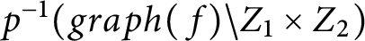 $p^{-1}(graph(\,f)\setminus Z_1\times Z_2)$
is coisotropic in X (since p is a Poisson diffeomorphism away from the exceptional divisor), and the same holds for its closure.
$p^{-1}(graph(\,f)\setminus Z_1\times Z_2)$
is coisotropic in X (since p is a Poisson diffeomorphism away from the exceptional divisor), and the same holds for its closure.
To finish the proof, we have to show that
 $\overline {\overline {graph(\,f)}}$
is transverse to the exceptional divisor
$\overline {\overline {graph(\,f)}}$
is transverse to the exceptional divisor
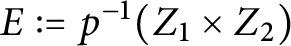 $E:=p^{-1}(Z_1\times Z_2)$
. Let
$E:=p^{-1}(Z_1\times Z_2)$
. Let
 $(x^{(1)}_{i})$
be local coordinates on
$(x^{(1)}_{i})$
be local coordinates on
 $M_1$
such that
$M_1$
such that
 $Z_1=\{x^{(1)}_{1}=0\}$
, and similarly, let
$Z_1=\{x^{(1)}_{1}=0\}$
, and similarly, let
 $(x^{(2)}_{j})$
be local coordinates on
$(x^{(2)}_{j})$
be local coordinates on
 $M_2$
such that
$M_2$
such that
 $Z_2=\{x^{(2)}_{1}=0\}$
. Then
$Z_2=\{x^{(2)}_{1}=0\}$
. Then
 $$ \begin{align*} \big(x^{(1)}_{i},f^*(x^{(2)}_{j})-x^{(2)}_{j}\big) \end{align*} $$
are local coordinates on
 $M_1\times M_2$
that are adapted
$M_1\times M_2$
that are adapted
 $graph(\,f)$
, but also to
$graph(\,f)$
, but also to
 $$ \begin{align*}(Z_1\times Z_2)=\big\{x^{(1)}_{1}=0,f^*(x^{(2)}_{1})-x^{(2)}_{1}=0\big\}, \end{align*} $$
due to the hypothesis
 $f(Z_1)\subset Z_2$
. Hence, we can apply Lemma 2.9, which yields the desired transversality.▪
$f(Z_1)\subset Z_2$
. Hence, we can apply Lemma 2.9, which yields the desired transversality.▪
The proof of Proposition 2.8 uses the following statement, for which we could not find a reference in the literature.
Lemma 2.9 Let
 $m,n$
be non-negative integers. Consider
$m,n$
be non-negative integers. Consider
 ${\mathbb R}^{n+m}$
with standard coordinates
${\mathbb R}^{n+m}$
with standard coordinates
 $x_1,\dots ,x_n,y_1,\dots ,y_{m}$
, and the subspaces
$x_1,\dots ,x_n,y_1,\dots ,y_{m}$
, and the subspaces
 $$ \begin{align*} Z:=&\{0\}\times {\mathbb R}^{m},\\ S:=&\big({\mathbb R}^{k}\times \{0\}\big)\times \big({\mathbb R}^{l }\times \{0\}\big), \end{align*} $$
where
 $k\le n$
and
$k\le n$
and
 $ l\le m$
. Then, in the blow-up
$ l\le m$
. Then, in the blow-up
 $Bl_Z({\mathbb R}^{n+m})$
, the submanifold
$Bl_Z({\mathbb R}^{n+m})$
, the submanifold
 $\overline {\overline {S}}$
interesects transversely the exceptional divisor E.
$\overline {\overline {S}}$
interesects transversely the exceptional divisor E.
Proof We have
 $$ \begin{align*}Bl_Z({\mathbb R}^{n+m})=\overline{\Big\{\Big((x,y),[x]\Big): x\in {\mathbb R}^{n}\setminus\{0\}, y\in {\mathbb R}^{m}\Big\}}\;\subset {\mathbb R}^{n+m}\times {\mathbb R} P^{n-1},\end{align*} $$
where
 $[\cdot ]$
denotes the class in projective space. Notice that by taking the closure, we are adding exactly the exceptional divisor
$[\cdot ]$
denotes the class in projective space. Notice that by taking the closure, we are adding exactly the exceptional divisor
 $$ \begin{align*}E=\{0\}\times {\mathbb R}^{m}\times {\mathbb R} P^{n-1}.\end{align*} $$
We have
 $$ \begin{align*} \overline{\overline{S}}=\overline{\Big\{\Big((x_1,0,y_1,0),[(x_1,0)]\Big): x_1\in {\mathbb R}^{k}\setminus\{0\}, y_1\in {\mathbb R}^{l}\Big\}}. \end{align*} $$
By taking the closure we are adding exactly
 $$ \begin{align*}\{0\}\times \big({\mathbb R}^{l}\times\{0\}\big)\times {\mathbb R} P^{k-1}=\overline{\overline{S}}\cap E.\end{align*} $$
For every point
 $p\in \overline {\overline {S}}\cap E$
there is a curve of the form
$p\in \overline {\overline {S}}\cap E$
there is a curve of the form
 $$ \begin{align*}\gamma\colon t\longmapsto \big((tx_1,0,y_1,0),[(x_1,0)]\big)\end{align*} $$
lying in
 $\overline {\overline {S}}$
with
$\overline {\overline {S}}$
with
 $\gamma (0)=p$
, and clearly
$\gamma (0)=p$
, and clearly
 $\frac {d}{dt}|_0\gamma (t)\notin T_pE$
. Since
$\frac {d}{dt}|_0\gamma (t)\notin T_pE$
. Since
 $\frac {d}{dt}|_0\gamma (t)\in T_p\overline {\overline {S}}$
and E has codimension
$\frac {d}{dt}|_0\gamma (t)\in T_p\overline {\overline {S}}$
and E has codimension
 $1$
, we obtain
$1$
, we obtain
 $T_pE+T_p\overline {\overline {S}}=T_pBl_Z({\mathbb R}^{n+m})$
.▪
$T_pE+T_p\overline {\overline {S}}=T_pBl_Z({\mathbb R}^{n+m})$
.▪
Remark 2.10 One can show that for any pair of submanifolds L and S intersecting cleanly, around any point of the intersection there exist local coordinates of the ambient manifold M that are simultaneously adapted to both submanifolds. Lemma 2.9 then implies that, with the notation of the beginning of this subsection,
 $\overline {\overline {S}}$
intersects the hypersurface
$\overline {\overline {S}}$
intersects the hypersurface
 $p^{-1}(L)$
of
$p^{-1}(L)$
of
 $Bl_L(M)$
transversely.
$Bl_L(M)$
transversely.
2.3 b-coisotropic Embeddings and the b-Gotay Theorem
If
 $C\overset {i}{\hookrightarrow }(M,Z,\omega )$
is b-coisotropic, then Proposition 2.4 implies that
$C\overset {i}{\hookrightarrow }(M,Z,\omega )$
is b-coisotropic, then Proposition 2.4 implies that
 $(C,C\cap Z,^bi^*\omega )$
is b-presymplectic; i.e., the b-two-form
$(C,C\cap Z,^bi^*\omega )$
is b-presymplectic; i.e., the b-two-form
 ${}^bi^*\omega \in {}^{b}\Omega ^{2}(C)$
is closed of constant rank. Conversely, in this subsection, we prove that any b-presymplectic manifold embeds b-coisotropically into a b-symplectic manifold, which is unique up to neighborhood equivalence. In other words, we show a version of Gotay’s theorem for b-coisotropic submanifolds. For Lagrangian submanifolds, this becomes a version of Weinstein’s tubular neighborhood theorem, which was obtained in [Reference Kirchhoff-Lukat13, Theorem 5.18].
${}^bi^*\omega \in {}^{b}\Omega ^{2}(C)$
is closed of constant rank. Conversely, in this subsection, we prove that any b-presymplectic manifold embeds b-coisotropically into a b-symplectic manifold, which is unique up to neighborhood equivalence. In other words, we show a version of Gotay’s theorem for b-coisotropic submanifolds. For Lagrangian submanifolds, this becomes a version of Weinstein’s tubular neighborhood theorem, which was obtained in [Reference Kirchhoff-Lukat13, Theorem 5.18].
As a consequence, a b-coisotropic submanifold
 $C\subset (M,Z,\omega )$
determines
$C\subset (M,Z,\omega )$
determines
 $\omega\; $
(up to b-symplectomorphism) in a neighborhood of C. Notice that arbitrary coisotropic submanifolds of the log-symplectic manifold
$\omega\; $
(up to b-symplectomorphism) in a neighborhood of C. Notice that arbitrary coisotropic submanifolds of the log-symplectic manifold
 $(M,Z,\Pi )$
do not satisfy this property: for instance, Z is a coisotropic (even Poisson) submanifold, and by [Reference Guillemin, Miranda and Pires11], the additional data consisting of a certain element of
$(M,Z,\Pi )$
do not satisfy this property: for instance, Z is a coisotropic (even Poisson) submanifold, and by [Reference Guillemin, Miranda and Pires11], the additional data consisting of a certain element of
 $H^1_{\Pi }(Z)$
is necessary in order to determine the b-symplectic structure in a neighborhood of Z.
$H^1_{\Pi }(Z)$
is necessary in order to determine the b-symplectic structure in a neighborhood of Z.
Definition 2.11 A b-presymplectic form on a b-manifold is a b-two-form, which is closed and of constant rank.
Definition 2.12 Let
 $(M_{1},Z_{1},\omega )$
be a b-manifold endowed with a b-presymplectic form
$(M_{1},Z_{1},\omega )$
be a b-manifold endowed with a b-presymplectic form
 $\omega \in {}^{b}\Omega ^{2}(M_{1})$
. A
b-coisotropic embedding of
$\omega \in {}^{b}\Omega ^{2}(M_{1})$
. A
b-coisotropic embedding of
 $M_{1}$
into a b-symplectic manifold
$M_{1}$
into a b-symplectic manifold
 $(M_{2},Z_{2},\Omega )$
is a b-map
$(M_{2},Z_{2},\Omega )$
is a b-map
 $\phi \colon (M_{1},Z_{1})\rightarrow (M_{2},Z_{2})$
such that
$\phi \colon (M_{1},Z_{1})\rightarrow (M_{2},Z_{2})$
such that
 $\phi $
is an embedding and
$\phi $
is an embedding and
-
(i)
${}^{b}\phi ^{*}\Omega =\omega $
; -
(ii)
$\phi (M_{1})$
is b-coisotropic in
$(M_{2},Z_{2},\Omega )$
.
We will prove the following Gotay theorem in the b-symplectic setting.
Theorem 2.13 (The b-Gotay theorem). Let
 $(C,Z_{C},\omega _{C})$
be a b-manifold with a b-presymplectic form
$(C,Z_{C},\omega _{C})$
be a b-manifold with a b-presymplectic form
 $\omega _{C}\in {}^{b}\Omega ^{2}(C)$
. We then have the following:
$\omega _{C}\in {}^{b}\Omega ^{2}(C)$
. We then have the following:
-
(a) C embeds b-coisotropically into a b-symplectic manifold;
-
(b) the embedding is unique up to b-symplectomorphism in a tubular neighborhood of C, fixing C pointwise.
We divide the proof of Theorem 2.13 into several steps. We roughly follow the reasoning from the symplectic case presented in [Reference Gotay8]. We start by constructing a b-symplectic thickening of the b-presymplectic manifold C, from which Theorem 2.13(a) will follow.
Proposition 2.14 Denote by E the vector bundle
 $\text{Ker}(\omega _{C})\subset {}^{b}TC$
. Then there is a b-symplectic structure
$\text{Ker}(\omega _{C})\subset {}^{b}TC$
. Then there is a b-symplectic structure
 $\Omega _G$
on a neighborhood of the zero section
$\Omega _G$
on a neighborhood of the zero section
 $C\subset E^{*}$
.
$C\subset E^{*}$
.
Proof Fix a complement G to E in
 ${}^{b}TC$
, and let
${}^{b}TC$
, and let
 $j\colon E^{*}\hookrightarrow {}^{b}T^{*}C$
be the induced inclusion. It is clear that
$j\colon E^{*}\hookrightarrow {}^{b}T^{*}C$
be the induced inclusion. It is clear that
 $j(E^{*})=G^{0}$
. Since both the bundle projection
$j(E^{*})=G^{0}$
. Since both the bundle projection
 $\pi \colon (E^{*},E^{*}|_{Z_{C}})\rightarrow (C,Z_{C})$
and the inclusion
$\pi \colon (E^{*},E^{*}|_{Z_{C}})\rightarrow (C,Z_{C})$
and the inclusion
 $j\colon (E^{*},E^{*}|_{Z_{C}})\rightarrow ({}^{b}T^{*}C,{}^{b}T^{*}C|_{Z_{C}})$
are b-maps, we can define a b-two-form
$j\colon (E^{*},E^{*}|_{Z_{C}})\rightarrow ({}^{b}T^{*}C,{}^{b}T^{*}C|_{Z_{C}})$
are b-maps, we can define a b-two-form
 $\Omega _{G}$
on
$\Omega _{G}$
on
 $(E^{*},E^{*}|_{Z_{C}})$
by
$(E^{*},E^{*}|_{Z_{C}})$
by
 $$ \begin{align} \Omega_{G}:={}^{b}\pi^{*}\omega_{C}+{}^{b}j^{*}\omega_{{can}}. \end{align} $$
Here,
 $\omega _{{can}}$
denotes the canonical b-symplectic form on
$\omega _{{can}}$
denotes the canonical b-symplectic form on
 ${}^{b}T^{*}C$
as in Example 1.17, and the subscript G is used to stress that the definition depends on the choice of complement G.
${}^{b}T^{*}C$
as in Example 1.17, and the subscript G is used to stress that the definition depends on the choice of complement G.
We want to show that
 $\Omega _{G}$
is b-symplectic on a neighborhood of
$\Omega _{G}$
is b-symplectic on a neighborhood of
 $C\subset (E^{*},E^{*}|_{Z_{C}})$
. As
$C\subset (E^{*},E^{*}|_{Z_{C}})$
. As
 $\Omega _{G}$
is clearly b-closed, it suffices to prove that
$\Omega _{G}$
is clearly b-closed, it suffices to prove that
 $\Omega _{G}$
is non-degenerate at points
$\Omega _{G}$
is non-degenerate at points
 $p\in C$
.
$p\in C$
.
We claim that under the decomposition
 $$\begin{align*}{}^{b}T_{p}({}^{b}T^{*}C)\cong{}^{b}T_{p}C\oplus{}^{b}T_{p}^{*}C, \end{align*}$$
of Lemma 1.12, the canonical b-symplectic form is the usual pairing
 $$ \begin{align} (\omega_{{can}})_{p}(v+\alpha,w+\beta)=\langle v,\beta\rangle - \langle w,\alpha\rangle. \end{align} $$
This claim can be checked writing in cotangent coordinates
 $ \omega _{{can}}=\frac {dx_{1}}{x_{1}}\wedge dy_{1}+\sum _{i=2}^{n}dx_{i}\wedge dy_{i}, $
and noticing that
$ \omega _{{can}}=\frac {dx_{1}}{x_{1}}\wedge dy_{1}+\sum _{i=2}^{n}dx_{i}\wedge dy_{i}, $
and noticing that
 $y_{i}$
is a linear coordinate on each fiber
$y_{i}$
is a linear coordinate on each fiber
 ${}^{b}T_{p}^{*}C$
, i.e.,
${}^{b}T_{p}^{*}C$
, i.e.,
 $y_{i}\in ({}^{b}T_{p}^{*}C)^{*}\cong {}^{b}T_{p}C$
.
$y_{i}\in ({}^{b}T_{p}^{*}C)^{*}\cong {}^{b}T_{p}C$
.
Consider now the decomposition
 $$ \begin{align} {}^{b}T_{p}E^{*}\cong{}^{b}T_{p}C\oplus E_{p}^{*}= E_{p}\oplus G_{p}\oplus E_{p}^{*} \end{align} $$
given by Lemma 1.12. Using Lemma 1.13(ii), we have
 $({}^{b}j_{*})_{p}= \text{Id} _{ {}^{b}T_{p}C}\oplus j|_{E_{p}^{*}}$
. Hence, under decomposition (2.8), we have
$({}^{b}j_{*})_{p}= \text{Id} _{ {}^{b}T_{p}C}\oplus j|_{E_{p}^{*}}$
. Hence, under decomposition (2.8), we have
 $$ \begin{align*} ({}^{b}j^{*}\omega_{{can}})_{p}(v+w+\alpha,x+y+\beta)&=\big(\omega_{{can}})_{p}(v+w+j(\alpha),x+y+j(\beta)\big)\\ &=\langle v+w,j(\beta)\rangle - \langle x+y,j(\alpha)\rangle\\ &=\langle v,j(\beta)\rangle-\langle x,j(\alpha)\rangle, \end{align*} $$
using the above claim and recalling that
 $j(E_{p}^{*})=G_{p}^{0}$
. In matrix notation,
$j(E_{p}^{*})=G_{p}^{0}$
. In matrix notation,

for some matrix A of full rank. Similarly, we have
 $({}^{b}\pi _{*})_{p}= \text{Id} _{ {}^{b}T_{p}C}\oplus 0$
, applying Lemma 1.13(ii) to
$({}^{b}\pi _{*})_{p}= \text{Id} _{ {}^{b}T_{p}C}\oplus 0$
, applying Lemma 1.13(ii) to
 $\pi $
(regarded as a vector bundle map). Therefore, under (2.8), we get
$\pi $
(regarded as a vector bundle map). Therefore, under (2.8), we get
 $$ \begin{align*} ({}^{b}\pi^{*}\omega_{C})_{p}(v+w+\alpha,x+y+\beta)=(\omega_{C})_{p}(v+w,x+y) \end{align*} $$
so that we get a matrix representation of the form

where we also use that
 $E=\text{Ker}(\omega _{C})$
. Note that the matrix B in (2.10) is of full rank, since the restriction of
$E=\text{Ker}(\omega _{C})$
. Note that the matrix B in (2.10) is of full rank, since the restriction of
 $(\omega _{C})_{p}$
to
$(\omega _{C})_{p}$
to
 $G_{p}$
is non-degenerate. Combining (2.9) and (2.10), we have that
$G_{p}$
is non-degenerate. Combining (2.9) and (2.10), we have that

which is of maximal rank. Therefore,
 $\Omega _{G}$
is non-degenerate at points
$\Omega _{G}$
is non-degenerate at points
 $p\in C\subset E^{*}$
.▪
$p\in C\subset E^{*}$
.▪
Proof Proof of Theorem 2.13(a)
We show that the inclusion
 $(C,Z_{C},\omega _{C})\overset {i}\hookrightarrow (E^{*},E^{*}|_{Z_{C}},\Omega _{G})$
is indeed a b-coisotropic embedding; i.e.,
$(C,Z_{C},\omega _{C})\overset {i}\hookrightarrow (E^{*},E^{*}|_{Z_{C}},\Omega _{G})$
is indeed a b-coisotropic embedding; i.e.,
-
(i)
${}^{b}i^{*}\Omega _{G}=\omega _{C}$
; -
(ii)
${}^{b}TC^{\Omega _{G}}\subset {}^{b}TC$
.
We have
 ${}^{b}i^{*}\Omega _{G}={}^{b}(\pi \circ i)^{*}\omega _{C}+{}^{b}(j\circ i)^{*}\omega _{\text{can}}=\omega _{C}+{}^{b}(j\circ i)^{*}\omega _{\text{can}}$
. Note that
${}^{b}i^{*}\Omega _{G}={}^{b}(\pi \circ i)^{*}\omega _{C}+{}^{b}(j\circ i)^{*}\omega _{\text{can}}=\omega _{C}+{}^{b}(j\circ i)^{*}\omega _{\text{can}}$
. Note that
 $j\circ i$
is the inclusion of C into
$j\circ i$
is the inclusion of C into
 ${}^{b}T^{*}C$
, so that
${}^{b}T^{*}C$
, so that
 ${}^{b}(j\circ i)^{*}\omega _{\text{can}}=0$
, since C is b-Lagrangian in
${}^{b}(j\circ i)^{*}\omega _{\text{can}}=0$
, since C is b-Lagrangian in
 $({}^{b}T^{*}C,\omega _{\text{can}})$
. This proves (i).
$({}^{b}T^{*}C,\omega _{\text{can}})$
. This proves (i).
To check (ii), we let
 $p\in C$
and choose
$p\in C$
and choose
 $v+w+\alpha \in E_{p}\oplus G_{p}\oplus E_{p}^{*}\cong {}^{b}T_{p}E^{*}$
lying in
$v+w+\alpha \in E_{p}\oplus G_{p}\oplus E_{p}^{*}\cong {}^{b}T_{p}E^{*}$
lying in
 ${}^{b}T_{p}C^{\Omega _{G}}$
. Let
${}^{b}T_{p}C^{\Omega _{G}}$
. Let
 $x\in E_{p}\subset {}^{b}T_{p}C$
be arbitrary. Thanks to (2.11), we then have
$x\in E_{p}\subset {}^{b}T_{p}C$
be arbitrary. Thanks to (2.11), we then have
 $$ \begin{align*} 0=(\Omega_{G})_{p}(x,v+w+\alpha)=(\Omega_{G})_{p}(x,\alpha), \end{align*} $$
which forces that
 $\alpha =0$
due to non-degeneracy of
$\alpha =0$
due to non-degeneracy of
 $(\Omega _{G})_{p}$
on
$(\Omega _{G})_{p}$
on
 $E_{p}\times E_{p}^{*}$
. Hence,
$E_{p}\times E_{p}^{*}$
. Hence,
 $v+w+\alpha =v+w$
lies in
$v+w+\alpha =v+w$
lies in
 $E_{p}\oplus G_{p}={}^{b}T_{p}C$
, as desired.▪
$E_{p}\oplus G_{p}={}^{b}T_{p}C$
, as desired.▪
The uniqueness statement of Theorem 2.13(b) is an immediate consequence of the following proposition, to which we devote the rest of this subsection.
Proposition 2.15 Let
 $(M,Z,\omega )$
be a b-symplectic manifold and let C be a b-coisotropic submanifold, with induced b-presymplectic form
$(M,Z,\omega )$
be a b-symplectic manifold and let C be a b-coisotropic submanifold, with induced b-presymplectic form
 $\omega _{C}\in {}^{b}\Omega ^{2}(C)$
. Let
$\omega _{C}\in {}^{b}\Omega ^{2}(C)$
. Let
 $E:=\text{Ker}(\omega _{C})$
and fix a splitting
$E:=\text{Ker}(\omega _{C})$
and fix a splitting
 ${}^{b}TC=E\oplus G$
. Then there is a b-symplectomorphism
${}^{b}TC=E\oplus G$
. Then there is a b-symplectomorphism
 $\tau $
between a neighborhood of
$\tau $
between a neighborhood of
 $C\subset (M,Z,\omega )$
and a neighborhood of
$C\subset (M,Z,\omega )$
and a neighborhood of
 $C\subset (E^{*},E^{*}|_{C\cap Z},\Omega _{G})$
, with
$C\subset (E^{*},E^{*}|_{C\cap Z},\Omega _{G})$
, with
 $\tau |_{C}= \text{Id} _{C}$
.
$\tau |_{C}= \text{Id} _{C}$
.
Proof Since
 $\omega |_{G\times G}$
is non-degenerate, we have a decomposition
$\omega |_{G\times G}$
is non-degenerate, we have a decomposition
 ${}^{b}TM|_{C}=G\oplus G^{\omega }$
as symplectic vector bundles. Note that E is a Lagrangian subbundle of
${}^{b}TM|_{C}=G\oplus G^{\omega }$
as symplectic vector bundles. Note that E is a Lagrangian subbundle of
 $(G^{\omega },\omega )$
, since
$(G^{\omega },\omega )$
, since
 $$ \begin{align} E^{\omega}\cap G^{\omega}=(E\oplus G)^{\omega}={}^{b}TC^{\omega}={}^{b}TC^{\omega}\cap{}^{b}TC=E. \end{align} $$
We fix a Lagrangian complement V to E in
 $(G^{\omega },\omega )$
, i.e.,
$(G^{\omega },\omega )$
, i.e.,
 $G^{\omega }=E\oplus V$
.
$G^{\omega }=E\oplus V$
.
The idea of the proof is to construct a b-diffeomorphism between neighborhoods of C in M and
 $E^*$
—obtained as a composition of b-diffeomorphisms to a neighborhood in V— whose b-derivative at points of C pulls back
$E^*$
—obtained as a composition of b-diffeomorphisms to a neighborhood in V— whose b-derivative at points of C pulls back
 $\Omega _{G}$
to
$\Omega _{G}$
to
 $\omega $
, and then apply a Moser argument.
$\omega $
, and then apply a Moser argument.
We start by establishing a b-geometry version of the tubular neighborhood theorem, in which V plays the role of the normal bundle to C.
Claim 2.16 There is a b-diffeomorphism
 $\phi $
between a neighborhood of C in
$\phi $
between a neighborhood of C in
 $(V,V|_{C\cap Z})$
and a neighborhood of C in
$(V,V|_{C\cap Z})$
and a neighborhood of C in
 $(M,Z)$
, satisfying
$(M,Z)$
, satisfying
 $\left .{}^{b}\phi _{*}\right |{}_{C}= \text{Id} _{{}^{b}TM|_{C}}$
.
$\left .{}^{b}\phi _{*}\right |{}_{C}= \text{Id} _{{}^{b}TM|_{C}}$
.
We will construct this map in two steps:
 $$\begin{align*}V\xrightarrow[(1)]{} \rho(V)\xrightarrow[(2)]{} M. \end{align*}$$
Step 1. Let
 $\rho \colon {}^{b}TM\rightarrow TM$
denote the anchor map of
$\rho \colon {}^{b}TM\rightarrow TM$
denote the anchor map of
 ${}^{b}TM$
and notice that its restriction to V is injective. To see this, recall the decomposition
${}^{b}TM$
and notice that its restriction to V is injective. To see this, recall the decomposition
 $$ \begin{align} {}^{b}TM|_{C}=G\oplus G^{\omega}=G\oplus E\oplus V={}^{b}TC\oplus V \end{align} $$
and the fact that
 $\text{Ker}(\rho |_{C})\subset {}^{b}TC$
by Lemma 1.8, so that
$\text{Ker}(\rho |_{C})\subset {}^{b}TC$
by Lemma 1.8, so that
 $\text{Ker}(\rho )$
intersects V trivially. As such, we get a b-diffeomorphism
$\text{Ker}(\rho )$
intersects V trivially. As such, we get a b-diffeomorphism
 $\rho \colon (V,V|_{C\cap Z})\rightarrow (\rho (V),\rho (V)|_{C\cap Z})$
.Step 2. The distribution
$\rho \colon (V,V|_{C\cap Z})\rightarrow (\rho (V),\rho (V)|_{C\cap Z})$
.Step 2. The distribution
 $\rho (V)$
is complementary to
$\rho (V)$
is complementary to
 $TC$
, i.e.,
$TC$
, i.e.,
 $$ \begin{align*} TM|_{C}=TC\oplus\rho(V). \end{align*} $$
Indeed, by Step 1, we have at any point
 $p\in C$
,
$p\in C$
,
 $$\begin{align*}\dim(T_{p}M)=\dim(T_{p}C)+\dim(V_{p}) =\dim(T_{p}C)+\dim(\rho(V_{p})), \end{align*}$$
and moreover, if
 $v\in V_{p}$
is such that
$v\in V_{p}$
is such that
 $\rho (v)\in T_{p}C$
, then
$\rho (v)\in T_{p}C$
, then
 $v\in {}^{b}T_{p}C\cap V_{p}=\{0\}$
. Now fix a Riemannian metric g on M such that
$v\in {}^{b}T_{p}C\cap V_{p}=\{0\}$
. Now fix a Riemannian metric g on M such that
 $Z\subset (M,g)$
is totally geodesic (e.g., [Reference Milnor19, Lemma 6.8]). The corresponding exponential map
$Z\subset (M,g)$
is totally geodesic (e.g., [Reference Milnor19, Lemma 6.8]). The corresponding exponential map
 $\exp _{g}$
takes a neighborhood of
$\exp _{g}$
takes a neighborhood of
 $C\subset \rho (V)$
diffeomorphically onto a neighborhood of
$C\subset \rho (V)$
diffeomorphically onto a neighborhood of
 $C\subset M$
. Moreover, the fibers of
$C\subset M$
. Moreover, the fibers of
 $\rho (V)$
over
$\rho (V)$
over
 $C\cap Z$
are mapped into Z, since
$C\cap Z$
are mapped into Z, since
 $\rho (V_{p})\in T_{p}Z$
for
$\rho (V_{p})\in T_{p}Z$
for
 $p\in C\cap Z$
and Z is totally geodesic. Therefore, the mapFootnote
2
$p\in C\cap Z$
and Z is totally geodesic. Therefore, the mapFootnote
2
 $\exp _{g}\colon (\rho (V),\rho (V)|_{C\cap Z})\rightarrow (M,Z)$
is a b-diffeomorphism between neighborhoods of C.
$\exp _{g}\colon (\rho (V),\rho (V)|_{C\cap Z})\rightarrow (M,Z)$
is a b-diffeomorphism between neighborhoods of C.
We now show that
 $\phi :=\exp _{g}\circ \rho \colon V\to M$
has the claimed property. That is, we show that
$\phi :=\exp _{g}\circ \rho \colon V\to M$
has the claimed property. That is, we show that
 $[{}^{b}(\exp _{g}\circ \rho )_{*}]|_{C}$
is the identity map on
$[{}^{b}(\exp _{g}\circ \rho )_{*}]|_{C}$
is the identity map on
 ${}^{b}TV|_{C}\cong {}^{b}TC\oplus V={}^{b}TM|_{C}$
, by checking that it acts as the identity on sections. We will need the commutative diagram
${}^{b}TV|_{C}\cong {}^{b}TC\oplus V={}^{b}TM|_{C}$
, by checking that it acts as the identity on sections. We will need the commutative diagram

which implicitly uses Lemma 1.13(i). We will also use that for all
 $q\in C$
the ordinary derivative reads
$q\in C$
the ordinary derivative reads
 $$ \begin{align} \big[(\exp_{g}\circ\rho)_{\ast}\big]_{q}\colon T_{q}V\cong T_{q}C\oplus V_{q} & \longrightarrow T_{q}M = T_{q}C\oplus\rho(V_{q})\nonumber \\ w+v & \longmapsto w+\rho(v). \end{align} $$
For a section
 $X+Y\in \Gamma ({}^{b}TC\oplus V)$
, we now compute
$X+Y\in \Gamma ({}^{b}TC\oplus V)$
, we now compute
 $$ \begin{align*} \rho[{}^{b}(\exp_{g}\circ\rho)_{*}(X+Y)]&=(\exp_{g}\circ\rho)_{*}(\rho(X)+Y)\\ &=\rho(X)+\rho(Y)\\ &=\rho(X+Y), \end{align*} $$
using (2.14) in the first equality and (2.15) in the second. Since the anchor
 $\rho $
is injective on sections, this implies that
$\rho $
is injective on sections, this implies that
 ${}^{b}(\exp _{g}\circ \rho )_{*}(X+Y)=X+Y$
, as desired. Claim 2.16 is proved.
${}^{b}(\exp _{g}\circ \rho )_{*}(X+Y)=X+Y$
, as desired. Claim 2.16 is proved.
Next, the map
 $$ \begin{align*} \psi\colon V\longrightarrow E^{*},\quad v\longmapsto -\iota_{v}\omega|_{E} \end{align*} $$
is an isomorphism of vector bundles covering
 $ \text{Id} _{C}$
, whence a b-diffeomorphism between the total spaces (\,For the injectivity, note that
$ \text{Id} _{C}$
, whence a b-diffeomorphism between the total spaces (\,For the injectivity, note that
 $ \iota _{v}\omega |_{E}=0$
implies that
$ \iota _{v}\omega |_{E}=0$
implies that
 $v\in E^{\omega }\cap G^{\omega }=E$
as in (2.12), so that
$v\in E^{\omega }\cap G^{\omega }=E$
as in (2.12), so that
 $v\in V\cap E=\{0\}$
). The composition
$v\in V\cap E=\{0\}$
). The composition
 $\psi \circ \phi ^{-1}\colon (M,Z)\rightarrow (E^{*},E^{*}|_{C\cap Z})$
is a b-diffeomorphism between neighborhoods of C, with
$\psi \circ \phi ^{-1}\colon (M,Z)\rightarrow (E^{*},E^{*}|_{C\cap Z})$
is a b-diffeomorphism between neighborhoods of C, with
 $(\psi \circ \phi ^{-1})|_{C}= \text{Id} _{C}$
.
$(\psi \circ \phi ^{-1})|_{C}= \text{Id} _{C}$
.
Claim 2.17 This b-diffeomorphism satisfies
 $\left .\left [{}^{b}(\psi \circ \phi ^{-1})^{*}\Omega _{G}\right ]\right |{}_{C}=\left .\omega \right |{}_{C}$
.
$\left .\left [{}^{b}(\psi \circ \phi ^{-1})^{*}\Omega _{G}\right ]\right |{}_{C}=\left .\omega \right |{}_{C}$
.
As before, let
 $\pi \colon E^{*}\rightarrow C$
denote the bundle projection, and let
$\pi \colon E^{*}\rightarrow C$
denote the bundle projection, and let
 $j\colon E^{*}\hookrightarrow {}^{b}T^{*}C$
be the inclusion induced by the splitting
$j\colon E^{*}\hookrightarrow {}^{b}T^{*}C$
be the inclusion induced by the splitting
 ${}^{b}TC=E\oplus G$
. Since
${}^{b}TC=E\oplus G$
. Since
 $\psi \colon V\rightarrow E^{*}$
is a vector bundle morphism covering
$\psi \colon V\rightarrow E^{*}$
is a vector bundle morphism covering
 $ \text{Id} _C$
, by Lemma 1.13(ii), we have that
$ \text{Id} _C$
, by Lemma 1.13(ii), we have that
 $$ \begin{align*} {}^{b}\psi_{*}|_C\colon {}^{b}TV|_C\cong{}^{b}TC\oplus V\longrightarrow {}^{b}TE^*|_C\cong{}^{b}TC\oplus E^* \end{align*} $$
equals
 $ \text{Id}_{^{b}TC} \oplus \psi $
. Furthermore,
$ \text{Id}_{^{b}TC} \oplus \psi $
. Furthermore,
 ${}^{b}\phi _{*}|_{C}= \text{Id} _{{}^{b}TM|_{C}}$
by Claim 2.16. Therefore, for
${}^{b}\phi _{*}|_{C}= \text{Id} _{{}^{b}TM|_{C}}$
by Claim 2.16. Therefore, for
 $p\in C$
and
$p\in C$
and
 $x_i+v_i\in {}^{b}T_pC \oplus V_{p}={}^{b}T_{p}M$
, we have
$x_i+v_i\in {}^{b}T_pC \oplus V_{p}={}^{b}T_{p}M$
, we have
 $$ \begin{align} \big[{}^{b}(\psi\circ\phi^{-1})^{*}\Omega_{G}\big]_{p}(x_{1}+v_{1},x_{2}+v_{2})=(\Omega_{G})_{p}\big(x_{1}+\psi(v_{1}),x_{2}+\psi(v_{2})\big). \end{align} $$
Recalling equation (2.6) and applying Lemma 1.13(ii) as in the proof of Proposition 2.14, we expand the right-hand side of (2.16) as follows:
 $$ \begin{align*} (\Omega_{G})_{p}\big(x_{1}+\psi(v_{1}),x_{2}+\psi(v_{2})\big) & =\omega_{p}(x_{1},x_{2})+(\omega_{{can}})_{p}(x_{1}+j(\psi(v_{1})),x_{2}+j(\psi(v_{2})))\\ &=\omega_{p}(x_{1},x_{2})+\left\langle x_{1},j(\psi(v_{2}))\right\rangle-\left\langle x_{2},j(\psi(v_{1}))\right\rangle\\ &=\omega_{p}(x_{1},x_{2})+\langle e_{1},\psi(v_{2})\rangle - \langle e_{2},\psi(v_{1})\rangle\\ &=\omega_{p}(x_{1},x_{2})+\omega_{p}(e_{1},v_{2})+\omega_{p}(v_{1},e_{2})\\ &=\omega_{p}(x_{1}+v_{1},x_{2}+v_{2}), \end{align*} $$
using equation (2.7) in the second equality, writing
 $x_i=e_i+g_i\in E_{p}\oplus G_{p}={}^{b}T_{p}C$
, and using in the last equality that V is a Lagrangian subbundle of
$x_i=e_i+g_i\in E_{p}\oplus G_{p}={}^{b}T_{p}C$
, and using in the last equality that V is a Lagrangian subbundle of
 $(G^{\omega },\omega )$
. This finishes the proof of Claim 2.17.
$(G^{\omega },\omega )$
. This finishes the proof of Claim 2.17.
Applying Proposition 1.19 (relative b-Moser) yields a b-diffeomorphism
 $\sigma $
, defined on a neighborhood of
$\sigma $
, defined on a neighborhood of
 $C\subset (M,Z)$
, such that
$C\subset (M,Z)$
, such that
 ${}^{b}\sigma ^{*}({}^{b}(\psi \circ \phi ^{-1})^{*}\Omega _{G})=\omega $
and
${}^{b}\sigma ^{*}({}^{b}(\psi \circ \phi ^{-1})^{*}\Omega _{G})=\omega $
and
 $\sigma |_{C}= \text{Id} _{C}$
. So setting
$\sigma |_{C}= \text{Id} _{C}$
. So setting
 $\tau :=\psi \circ \phi ^{-1}\circ \sigma $
finishes the proof.▪
$\tau :=\psi \circ \phi ^{-1}\circ \sigma $
finishes the proof.▪
3 Strong b-coisotropic Submanifolds and b-symplectic Reduction
We consider a subclass of b-coisotropic submanifolds in b-symplectic manifolds, namely, the coisotropic submanifolds that are transverse to the symplectic leaves they meet. The main observation is that their characteristic distribution has constant rank, and the quotient (whenever smooth) by this distribution inherits a b-symplectic form (Proposition 3.6).
3.1 Strong b-coisotropic Submanifolds
In Subsection 2.1, we have seen that a b-coisotropic submanifold
 $C\subset (M,Z,\omega )$
comes with a characteristic distribution
$C\subset (M,Z,\omega )$
comes with a characteristic distribution
 $$ \begin{align*} D:=\rho({}^{b}TC^{\omega})=\Pi^{\sharp}(TC^{0}). \end{align*} $$
In general, D fails to be regular. To force D to have a constant rank, we have to impose a condition on C that is stronger than b-coisotropicity.
Definition 3.1 A submanifold C of a log-symplectic manifold
 $(M,Z,\Pi )$
is called strong b-coisotropic if it is coisotropic (with respect to
$(M,Z,\Pi )$
is called strong b-coisotropic if it is coisotropic (with respect to
 $\Pi $
) and transverse to all the symplectic leaves of
$\Pi $
) and transverse to all the symplectic leaves of
 $ (M,\Pi )$
it meets.
$ (M,\Pi )$
it meets.
To justify this definition, we note that
 $$ \begin{align} \Pi_{p}^{\sharp}|_{T_{p}C^{0}}\ \text{is injective}&\Leftrightarrow \text{Ker}(\Pi_{p}^{\sharp})\cap T_{p}C^{0}=\{0\}\nonumber\\ &\Leftrightarrow T_{p}\mathcal{O}^{0}\cap T_{p}C^{0}=\{0\}\nonumber\\ &\nonumber\Leftrightarrow (T_{p}\mathcal{O}+T_{p}C)^{0}=\{0\}\\ \ &\Leftrightarrow T_{p}\mathcal{O}+T_{p}C=T_{p}M, \end{align} $$
where
 $\mathcal {O}$
denotes the symplectic leaf through p. The last equation is exactly the transversality condition of Definition 3.1. Consequently, we have the following proposition.
$\mathcal {O}$
denotes the symplectic leaf through p. The last equation is exactly the transversality condition of Definition 3.1. Consequently, we have the following proposition.
Proposition 3.2 Let
 $C\subset (M,Z,\Pi )$
be a coisotropic submanifold. Then C is strong b-coisotropic if and only if the characteristic distribution of C is regular, with rank equal to
$C\subset (M,Z,\Pi )$
be a coisotropic submanifold. Then C is strong b-coisotropic if and only if the characteristic distribution of C is regular, with rank equal to
 ${codim}(C)$
.
${codim}(C)$
.
Lemma 2.5 immediately implies the following corollary.
Corollary 3.3 Let
 $C\subset (M,Z,\omega )$
be strong b-coisotropic. Then its characteristic distribution is tangent to Z, and corresponds to
$C\subset (M,Z,\omega )$
be strong b-coisotropic. Then its characteristic distribution is tangent to Z, and corresponds to
 ${}^{b}TC^{\omega } $
under the bijection of Lemma 1.10 (ii).
${}^{b}TC^{\omega } $
under the bijection of Lemma 1.10 (ii).
Remark 3.4 If C is a strong b-coisotropic submanifold of
 $(M^{2n},Z,\Pi )$
intersecting Z, then necessarily
$(M^{2n},Z,\Pi )$
intersecting Z, then necessarily
 $\dim (C)\geq n+1$
. Indeed, if
$\dim (C)\geq n+1$
. Indeed, if
 $\mathcal {O}$
denotes the symplectic leaf through
$\mathcal {O}$
denotes the symplectic leaf through
 $p\in C\cap Z$
, then we have
$p\in C\cap Z$
, then we have
 $$ \begin{align*} \dim(C)&=\dim(T_{p}\mathcal{O}+T_{p}C)+\dim(T_{p}\mathcal{O}\cap T_{p}C)-\dim(\mathcal{O})\\ &=\dim(T_{p}\mathcal{O}\cap T_{p}C)+2\\ &\geq n+1, \end{align*} $$
where the last inequality holds, since
 $T_{p}\mathcal {O}\cap T_{p}C$
is a coisotropic subspace of the
$T_{p}\mathcal {O}\cap T_{p}C$
is a coisotropic subspace of the
 $(2n-2)$
-dimensional vector space
$(2n-2)$
-dimensional vector space
 $T_{p}\mathcal {O}$
. Alternatively, one can observe that a middle-dimensional b-coisotropic submanifold
$T_{p}\mathcal {O}$
. Alternatively, one can observe that a middle-dimensional b-coisotropic submanifold
 $C^{n}\subset (M^{2n},Z,\omega )$
is b-Lagrangian (i.e.,
$C^{n}\subset (M^{2n},Z,\omega )$
is b-Lagrangian (i.e.,
 ${}^{b}TC^{\omega }={}^{b}TC$
). Its characteristic distribution satisfies
${}^{b}TC^{\omega }={}^{b}TC$
). Its characteristic distribution satisfies
 $$ \begin{align*} \dim(D_{p})=\left\{\begin{array}{ll} \dim(C)-1&\text{if}\; {p}\in {C}\cap Z,\\ \dim(C) &\text{else}, \end{array}\right. \end{align*} $$
so that C cannot be strong b-coisotropic whenever it intersects Z, due to Proposition 3.2.
3.2 Coisotropic Reduction in b-symplectic Geometry
In this subsection we adapt coisotropic reduction to the b-symplectic category. It is well known that, given a coisotropic submanifold C of a Poisson manifold M, its quotient
 $\underline {C}$
by the characteristic distribution is again a Poisson manifold, provided it is smooth. More precisely, the vanishing ideal
$\underline {C}$
by the characteristic distribution is again a Poisson manifold, provided it is smooth. More precisely, the vanishing ideal
 $\mathcal {I}_{C}$
is a Poisson subalgebra of
$\mathcal {I}_{C}$
is a Poisson subalgebra of
 $(C^{\infty }(M),\{\cdot ,\cdot \})$
, and denoting by
$(C^{\infty }(M),\{\cdot ,\cdot \})$
, and denoting by
 $\mathcal {N}(\mathcal {I}_{C}):=\{\,f\in C^{\infty }(M): \{\,f,\; \mathcal {I}_{C}\}\subset \mathcal {I}_{C}\}$
its Poisson normalizer,\;we have that
$\mathcal {N}(\mathcal {I}_{C}):=\{\,f\in C^{\infty }(M): \{\,f,\; \mathcal {I}_{C}\}\subset \mathcal {I}_{C}\}$
its Poisson normalizer,\;we have that
 $\;\mathcal {N}(\mathcal {I}_{C})/\mathcal {I}_{C}$
is a Poisson algebra. As an algebra, it is canonically isomorphic to the algebra of smooth functions on the quotient
$\;\mathcal {N}(\mathcal {I}_{C})/\mathcal {I}_{C}$
is a Poisson algebra. As an algebra, it is canonically isomorphic to the algebra of smooth functions on the quotient
 $\underline {C}$
, so it endows the latter with a Poisson structure, called the reduced Poisson structure.
$\underline {C}$
, so it endows the latter with a Poisson structure, called the reduced Poisson structure.
Remark 3.5 When the Poisson structure on M is non-degenerate, i.e., corresponds to a symplectic form
 $\omega \in \Omega ^2(M)$
, the reduced Poisson structure on
$\omega \in \Omega ^2(M)$
, the reduced Poisson structure on
 $\underline {C}$
is also non-degenerate. Indeed [Reference Śniatycki and Weinstein22], it corresponds to the symplectic form
$\underline {C}$
is also non-degenerate. Indeed [Reference Śniatycki and Weinstein22], it corresponds to the symplectic form
 $\omega _{\text{red}}$
on
$\omega _{\text{red}}$
on
 $\underline {C}$
obtained by symplectic coisotropic reduction, i.e., the unique one that satisfies
$\underline {C}$
obtained by symplectic coisotropic reduction, i.e., the unique one that satisfies
 $q^*\omega _{\text{red}}=i^*\omega $
, where
$q^*\omega _{\text{red}}=i^*\omega $
, where
 $q\colon\; C\to \underline {C}$
is the projection, and
$q\colon\; C\to \underline {C}$
is the projection, and
 $i\colon\; C\to M$
is the inclusion.
$i\colon\; C\to M$
is the inclusion.
Proposition 3.6 (Coisotropic reduction). Let C be a strong b-coisotropic submanifold of a b-symplectic manifold
 $(M,Z,\omega ,\Pi )$
. Then
$(M,Z,\omega ,\Pi )$
. Then
 $D:=\Pi ^{\sharp }(TC^{0})$
is a (constant rank) involutive distribution on C. Assume that
$D:=\Pi ^{\sharp }(TC^{0})$
is a (constant rank) involutive distribution on C. Assume that
 $\underline {C}:=C/D$
has a smooth manifold structure, such that the projection
$\underline {C}:=C/D$
has a smooth manifold structure, such that the projection
 $q\colon C\rightarrow \underline {C}$
is a submersion. Then
$q\colon C\rightarrow \underline {C}$
is a submersion. Then
 $\underline {C}$
inherits a b-symplectic structure
$\underline {C}$
inherits a b-symplectic structure
 $\underline {\Omega }$
, determined by
$\underline {\Omega }$
, determined by
 $$ \begin{align} {}^{b}q^{*}\underline{\Omega}={}^{b}i^{*}\omega, \end{align} $$
where
 $i\colon C\hookrightarrow M$
is the inclusion. Its corresponding log-symplectic structure is exactly the reduced Poisson structure on
$i\colon C\hookrightarrow M$
is the inclusion. Its corresponding log-symplectic structure is exactly the reduced Poisson structure on
 $\underline {C}$
obtained from
$\underline {C}$
obtained from
 $\Pi $
.
$\Pi $
.
Proof We know that D has constant rank, by Proposition 3.2. As for involutivity, first note that D is generated by Hamiltonians
 $\left .X_{h}\right |{}_{C}$
of functions
$\left .X_{h}\right |{}_{C}$
of functions
 $h\in \mathcal {I}_{C}$
. On such generators, we have
$h\in \mathcal {I}_{C}$
. On such generators, we have
 $$ \begin{align*} [X_{h_{1}}|_{C},X_{h_{2}}|_{C}]=[X_{h_{1}},X_{h_{2}}]|_{C}= X_{\{h_{1},h_{2}\}} |_{C}, \end{align*} $$
where
 $\{h_{1},h_{2}\}\in \mathcal {I}_{C}$
due to coisotropicity of C. Hence, D is involutive.
$\{h_{1},h_{2}\}\in \mathcal {I}_{C}$
due to coisotropicity of C. Hence, D is involutive.
The quotient
 $\underline {C\cap Z}:=(C\cap Z)/D$
is a smooth submanifold of
$\underline {C\cap Z}:=(C\cap Z)/D$
is a smooth submanifold of
 $\underline {C}$
, since for every slice S in C transverse to D, the intersection
$\underline {C}$
, since for every slice S in C transverse to D, the intersection
 $S\cap Z$
is a smooth slice in
$S\cap Z$
is a smooth slice in
 $C\cap Z$
transverse to D. The leaf space
$C\cap Z$
transverse to D. The leaf space
 $(\underline {C},\underline {C\cap Z})$
is a b-manifold, and the projection
$(\underline {C},\underline {C\cap Z})$
is a b-manifold, and the projection
 $q:(C,C\cap Z)\rightarrow (\underline {C},\underline {C\cap Z})$
is a b-map. For
$q:(C,C\cap Z)\rightarrow (\underline {C},\underline {C\cap Z})$
is a b-map. For
 $p\in C$
, we have an exact sequence
$p\in C$
, we have an exact sequence
 $$\begin{align*}0\longrightarrow D_{p}\hookrightarrow T_{p}C\overset{(q_{*})_{p}}{\longrightarrow} T_{q(p)}\underline{C}\longrightarrow 0, \end{align*}$$
which corresponds with an exact sequence on the level of b-tangent spaces
 $$ \begin{align} 0\longrightarrow({}^{b}T_{p}C)^{\omega_{p}}\hookrightarrow{}^{b}T_{p}C\overset{({}^{b}q_{*})_{p}}{\longrightarrow}{}^{b}T_{q(p)}\underline{C}\longrightarrow 0. \end{align} $$
To see this, consider the canonical splitting
 $\sigma \colon D\rightarrow {}^{b}TC$
of the anchor
$\sigma \colon D\rightarrow {}^{b}TC$
of the anchor
 $\rho \colon {}^{b}TC\rightarrow TC$
, as constructed in Lemma 1.10(i), and notice that
$\rho \colon {}^{b}TC\rightarrow TC$
, as constructed in Lemma 1.10(i), and notice that
 $$ \begin{align*} \text{Ker}\big(({}^b q_{*})\big)_p=\sigma(\text{Ker}(q_{*})_{p})=\sigma(D_{p})=({}^{b}T_{p}C)^{\omega_{p}}, \end{align*} $$
where the first equality holds by Corollary 1.11 and the third by Corollary 3.3.
Since q is a surjective submersion, it admits sections; hence, for every sufficiently small open subset
 $U\subset \underline {C}$
, there is a submanifold
$U\subset \underline {C}$
, there is a submanifold
 $S\subset C$
transverse to D such that
$S\subset C$
transverse to D such that
 $q|_{S}\colon S\to U$
is a diffeomorphism. At points
$q|_{S}\colon S\to U$
is a diffeomorphism. At points
 $p\in S$
, we have
$p\in S$
, we have
 $$ \begin{align*} {}^{b}T_{p}C =({}^{b}T_{p}C)^{\omega_{p}}\oplus{}^{b}T_{p}S \end{align*} $$
due to sequence (3.3). This implies that
 ${}^{b}i_{S}^{*}\omega _{C}$
is a b-symplectic form on S, where
${}^{b}i_{S}^{*}\omega _{C}$
is a b-symplectic form on S, where
 $i_{S}\colon S\hookrightarrow C$
is the inclusion and
$i_{S}\colon S\hookrightarrow C$
is the inclusion and
 $\omega _{C}$
is the restriction of
$\omega _{C}$
is the restriction of
 $\omega $
to C. Denote by
$\omega $
to C. Denote by
 $\tau \colon U\rightarrow S$
the inverse of
$\tau \colon U\rightarrow S$
the inverse of
 $q|_{S}\colon S\rightarrow U$
. Then
$q|_{S}\colon S\rightarrow U$
. Then
 $\underline {\Omega }:={}^{b}\tau ^{*}({}^{b}i_{S}^{*}\omega _{C})$
is b-symplectic on U. Away from
$\underline {\Omega }:={}^{b}\tau ^{*}({}^{b}i_{S}^{*}\omega _{C})$
is b-symplectic on U. Away from
 $\underline {C\cap Z}$
, this b-2-form agrees with the symplectic form obtained by symplectic coisotropic reduction from
$\underline {C\cap Z}$
, this b-2-form agrees with the symplectic form obtained by symplectic coisotropic reduction from
 $\omega |_{M\setminus Z}$
. Denote by
$\omega |_{M\setminus Z}$
. Denote by
 $-\underline {\Omega }^{-1}$
the non-degenerate b-bivector on U corresponding to
$-\underline {\Omega }^{-1}$
the non-degenerate b-bivector on U corresponding to
 $\underline {\Omega }$
. Away from
$\underline {\Omega }$
. Away from
 $\underline {C\cap Z}$
, the log-symplectic structure
$\underline {C\cap Z}$
, the log-symplectic structure
 $\underline {\rho }(-\underline {\Omega }^{-1})$
agrees with the reduced Poisson structure, by Remark 3.5. By continuity, the same is true on the whole of U. As U was arbitrary, the reduced Poisson structure on
$\underline {\rho }(-\underline {\Omega }^{-1})$
agrees with the reduced Poisson structure, by Remark 3.5. By continuity, the same is true on the whole of U. As U was arbitrary, the reduced Poisson structure on
 $\underline {C}$
is log-symplectic, and the above reasoning shows that the corresponding b-symplectic form satisfies equation (3.2).▪
$\underline {C}$
is log-symplectic, and the above reasoning shows that the corresponding b-symplectic form satisfies equation (3.2).▪
Examples 3.7
-
(i) Let
$i\colon B\hookrightarrow (M,Z)$
be a b-submanifold. A quick check in coordinates showsFootnote
3
that
${}^bT^*M|_B$
is strong b-coisotropic in
${}^bT^*M$
. Its quotient
$\underline {{}^{b}T^{*}M|_B}$
is canonically b-symplectomorphic to
${}^{b}T^{*}B$
. To see this, consider the surjective submersion and notice that the fibers of
$$ \begin{align*} \varphi\colon {}^{b}T^*M|_B\longrightarrow{}^{b}T^{*}B \colon \alpha_{p}\longmapsto ({}^{b}i_{*})_{p}^{*}\alpha_{p} \end{align*} $$
$\varphi $
coincide with the leaves of the characteristic distribution on
${}^bT^*M|_B$
. So we get a b-diffeomorphism
$\overline {\varphi }\colon \underline {{}^bT^*M|_B}\rightarrow {}^{b}T^{*}B$
. To see that this is in fact a b-symplectomorphism, we note that the tautological b-one-forms on
${}^{b}T^{*}M$
and
${}^{b}T^{*}B$
are related by (3.4)where
$$ \begin{align} {}^{b}\varphi^{*}\theta_{B} ={}^{b}j^{*}\theta_{M}, \end{align} $$
$j\colon ^bT^*M|_B\hookrightarrow {}^{b}T^{*}M$
is the inclusion. Recall that the b-symplectic form
$\underline {\Omega }$
on
$\underline {{}^bT^*M|_B}$
is determined by the relation
${}^{b}q^{*}\underline {\Omega }={}^{b}j^{*}\omega _{M}$
, where
$q\colon ^bT^*M|_B\rightarrow \underline {{}^bT^*M|_B}$
is the projection (cf. (3.2)). Hence to conclude that
$\overline {\varphi }$
is b-symplectic, we have to show that
${}^{b}q^{*}({}^{b}\overline {\varphi }^{*}\omega _{B})={}^{b}j^{*}\omega _{M}$
. But this is immediate from (3.4) since
$\overline {\varphi }\circ q=\varphi $
.
-
(ii) Given a b-manifold
$(M,Z)$
, let K be a distribution on M tangent to Z. Thanks to Lemma 1.10(i), we can view K as a subbundle
$\sigma (K)$
of
${}^bTM$
. Its annihilator
$\sigma (K)^{0}$
is strong b-coisotropic in
${}^bT^*M$
, and the quotient
$\underline {\sigma (K)^{0}}$
is
${}^bT^*(M/K)$
, whenever
$M/K$
is smooth. We give a proof of this fact in the particular case of a Hamiltonian group action; see Corollary 3.13.


3.3 Moment Map Reduction in b-symplectic Geometry
Recall that, given an action of a Lie group G on a Poisson manifold
 $(M,\Pi )$
, a moment map is a Poisson map
$(M,\Pi )$
, a moment map is a Poisson map
 $J\colon M\rightarrow \mathfrak {g}^{*}$
satisfying
$J\colon M\rightarrow \mathfrak {g}^{*}$
satisfying
 $$ \begin{align} \Pi^{\sharp}(dJ^{x})=v_{x}\forall x\in\mathfrak{g}. \end{align} $$
Here,
 $J^{x}\colon M\rightarrow \mathbb {R}\colon p\mapsto \langle J(p),x\rangle $
is the x-component of J, the vector field
$J^{x}\colon M\rightarrow \mathbb {R}\colon p\mapsto \langle J(p),x\rangle $
is the x-component of J, the vector field
 $v_{x}$
is the infinitesimal generator of the action corresponding with
$v_{x}$
is the infinitesimal generator of the action corresponding with
 $x\in \mathfrak {g}$
, i.e.,
$x\in \mathfrak {g}$
, i.e.,
 $$ \begin{align*} {v_{x}(p)= \frac{d}{dt}|_{t=0}\exp(-tx)\cdot p,} \end{align*} $$
and
 $\mathfrak {g}^{*}$
is endowed with its canonical Lie-Poisson structure [Reference Cannas da Silva and Weinstein4, Section 3]. A G-equivariant map
$\mathfrak {g}^{*}$
is endowed with its canonical Lie-Poisson structure [Reference Cannas da Silva and Weinstein4, Section 3]. A G-equivariant map
 $J\colon M\rightarrow \mathfrak {g}^{*}$
satisfying (3.5) is automatically Poisson [Reference Vaisman23, Proposition 7.30].
$J\colon M\rightarrow \mathfrak {g}^{*}$
satisfying (3.5) is automatically Poisson [Reference Vaisman23, Proposition 7.30].
In view of Proposition 3.6, we recall a general fact about equivariant moment maps.
Lemma 3.8 Let G be a Lie group acting on a Poisson manifold
 $(M,\Pi )$
with equivariant moment map
$(M,\Pi )$
with equivariant moment map
 $J\colon M\rightarrow \mathfrak {g}^{*}$
. Assume the action is free on
$J\colon M\rightarrow \mathfrak {g}^{*}$
. Assume the action is free on
 $J^{-1}(0)$
. Then
$J^{-1}(0)$
. Then
-
(i)
$J^{-1}(0)$
is a coisotropic submanifold of
$(M,\Pi )$
; -
(ii)
$J^{-1}(0)$
is transverse to all symplectic leaves of
$(M,\Pi )$
it meets; -
(iii) the characteristic distribution
$\Pi ^{\sharp }(T(J^{-1}(0))^{0})$
on
$J^{-1}(0)$
coincides with the tangent distribution to the orbits of
$G\curvearrowright J^{-1}(0)$
.


Remark 3.9 (i) When
 $(M,\Pi )$
is a log-symplectic manifold, Lemma 3.8 implies that the level set
$(M,\Pi )$
is a log-symplectic manifold, Lemma 3.8 implies that the level set
 $J^{-1}(0)$
is a strong b-coisotropic submanifold.
$J^{-1}(0)$
is a strong b-coisotropic submanifold.
(ii) When G a torus, there is a more flexible notion of moment map [Reference Guillemin, Miranda, Pires and Scott12, Definition 22] for log-symplectic manifolds. The smooth level sets of such moment maps are not strong b-coisotropic submanifolds in general. Indeed, they can even fail to be transverse to the degeneracy locus Z (see [Reference Guillemin, Miranda, Pires and Scott12, Example 23] for an instance where Z itself is such a level set).
For the sake of for completeness, we provide a proof of Lemma 3.8. Items (i) and (iii) also follow from well-known facts in symplectic geometry, by restricting the G-action to each symplectic leaf (whenever G is connected) and using item (ii).
Proof
-
(i) We show that
$0$
is a regular value of J. Choosing
$p\in J^{-1}(0)$
, it is enough to prove that the restriction
$d_{p}J\; \colon\; Im (\Pi _{p}^{\sharp })\subset T_{p}M\rightarrow \mathfrak {g}^{*}$
is surjective. To this end, assume that
$\xi \in \mathfrak {g}$
annihilates
$d_{p}J(Im (\Pi _{p}^{\sharp }))$
. We then get for all
$\alpha \in T_{p}^{*}M$
that and therefore
$$ \begin{align*} \left\langle\alpha,(v_{\xi})_{p}\right\rangle=\left\langle\alpha,\Pi_{p}^{\sharp}(d_{p}J^{\xi})\right\rangle=-\left\langle d_{p}J^{\xi},\Pi_{p}^{\sharp}(\alpha)\right\rangle=-\left\langle d_{p}J(\Pi_{p}^{\sharp}(\alpha)),\xi\right\rangle=0, \end{align*} $$
$(v_{\xi })_{p}=0$
. Since the action
$G\curvearrowright J^{-1}(0)$
is free, this implies that
$\xi =0$
. It follows that
$d_{p}J(Im (\Pi _{p}^{\sharp }))=\mathfrak {g}^{*}$
, so
$0$
is indeed a regular value of J. In particular,
$J^{-1}(0)$
is a submanifold of M. The coisotropicity of
$J^{-1}(0)$
follows since it is the preimage of a symplectic leaf
$\{0\}\subset \mathfrak {g}^{*}$
under a Poisson map.
-
(ii) Let
$\mathcal {O}$
denote the symplectic leaf through
$p\in J^{-1}(0)$
. By the computation (3.1), it suffices to prove that
$\Pi _{p}^{\sharp }|_{[T_{p}J^{-1}(0)]^{0}}$
is injective. Since
$0$
is a regular value, this annihilator is given by
$[T_{p}J^{-1}(0)]^{0}\nonumber =\{ d_{p}J^{x}: x\in \mathfrak {g}\}.$
We now have a composition of maps that is injective by freeness of
$$ \begin{align*} &\mathfrak{g}\longrightarrow \big[T_{p}J^{-1}(0)\big]^{0} \longrightarrow\Pi_{p}^{\sharp} \big(\big[T_{p}J^{-1}(0)\big]^{0}\big)\\ &x\longmapsto d_{p}J^{x}\longmapsto\Pi_{p}^{\sharp}(d_{p}J^{x})=(v_{x})_{p}, \end{align*} $$
$G\curvearrowright J^{-1}(0)$
. In particular,
$\Pi _{p}^{\sharp }|_{[T_{p}J^{-1}(0)]^{0}}$
is injective.
-
(iii) We have
which is exactly the tangent space of the G-orbit through p.▪
$$ \begin{align*} \Pi_{p}^{\sharp}\big([T_{p}J^{-1}(0)]^{0}\big)=\big\{ \Pi_{p}^{\sharp}(d_{p}J^{x}): x\in\mathfrak{g}\big\}=\big\{ (v_{x})_{p}: x\in\mathfrak{g}\big\}, \end{align*} $$


Combining Proposition 3.6 with Lemma 3.8, we obtain a moment map reduction statement in the b-symplectic category. The case
 $G=S^{1}$
was addressed in [Reference Gualtieri, Li, Pelayo and Ratiu10, Proposition 7.8].
$G=S^{1}$
was addressed in [Reference Gualtieri, Li, Pelayo and Ratiu10, Proposition 7.8].
Corollary 3.10 Moment map reduction
Consider an action of a connected Lie group G on a b-symplectic manifold
 $(M,Z,\Pi )$
with equivariant moment map
$(M,Z,\Pi )$
with equivariant moment map
 $J\colon M\to \mathfrak {g}^*$
. Assume the action is free and proper on
$J\colon M\to \mathfrak {g}^*$
. Assume the action is free and proper on
 $J^{-1}(0)$
. Then
$J^{-1}(0)$
. Then
 $J^{-1}(0)$
is a strong b-coisotropic submanifold, and its reduction
$J^{-1}(0)$
is a strong b-coisotropic submanifold, and its reduction
 $J^{-1}(0)/G$
is b-symplectic.
$J^{-1}(0)/G$
is b-symplectic.
Remark 3.11 The fact that
 $J^{-1}(0)/G$
is b-symplectic follows already from [Reference Marrero, Padrón and Rodríguez-Olmos16, Theorem 3.11], taking
$J^{-1}(0)/G$
is b-symplectic follows already from [Reference Marrero, Padrón and Rodríguez-Olmos16, Theorem 3.11], taking
 $A={}^{b}TM$
there. (The hypothesis made there, that
$A={}^{b}TM$
there. (The hypothesis made there, that
 $(J_*)_x\circ \rho _x\colon {}^{b}T_xM\to \mathfrak {g}^*$
has contant rank for all
$(J_*)_x\circ \rho _x\colon {}^{b}T_xM\to \mathfrak {g}^*$
has contant rank for all
 $x\in J^{-1}(0)$
, is satisfied, since
$x\in J^{-1}(0)$
, is satisfied, since
 $J^{-1}(0)$
is transverse to Z). In that reference, the authors developed a reduction theory for level sets of arbitrary regular values
$J^{-1}(0)$
is transverse to Z). In that reference, the authors developed a reduction theory for level sets of arbitrary regular values
 $\mu \in \mathfrak {g}^*$
satisfying the constant rank hypothesis; their statement is thus more general than the reduction statement in our Corollary 3.10.
$\mu \in \mathfrak {g}^*$
satisfying the constant rank hypothesis; their statement is thus more general than the reduction statement in our Corollary 3.10.
3.3.1 Exact b-symplectic Forms
As a particular case of the previous construction, we consider the b-symplectic analog of a well-known fact in symplectic geometry. Recall that, if a Lie group G acts on an exact symplectic manifold
 $(M,-d\theta )$
and
$(M,-d\theta )$
and
 $\theta $
is invariant under the action, then
$\theta $
is invariant under the action, then
 $J\colon M\rightarrow \mathfrak {g}^{*}$
defined by
$J\colon M\rightarrow \mathfrak {g}^{*}$
defined by
 $$ \begin{align} J^{x}=-\iota_{v_{x}}\theta \end{align} $$
is an equivariant moment map for the action (in the sense of (3.5)). For a proof, see, for instance, [Reference Abraham and Marsden1, Theorem 4.2.10]. A similar result holds in b-symplectic geometry.
Lemma 3.12 Exact b-symplectic forms
Suppose
 $(M,Z)$
is a b-manifold with exact b-symplectic form
$(M,Z)$
is a b-manifold with exact b-symplectic form
 $\omega =-{}^{b}d\theta $
. If
$\omega =-{}^{b}d\theta $
. If
 $\phi \colon G\times M\rightarrow M$
is a Lie group action preserving Z and
$\phi \colon G\times M\rightarrow M$
is a Lie group action preserving Z and
 $\theta \in {}^{b}\Omega ^{1}(M)$
, then an equivariant moment map
$\theta \in {}^{b}\Omega ^{1}(M)$
, then an equivariant moment map
 $J\colon M\rightarrow \mathfrak {g}^{*}$
is given by
$J\colon M\rightarrow \mathfrak {g}^{*}$
is given by
 $J^{x}=-\iota _{V_{x}}\theta $
. Here,
$J^{x}=-\iota _{V_{x}}\theta $
. Here,
 $V_{x}\in \Gamma ({}^{b}TM)$
is the lift of the infinitesimal generator
$V_{x}\in \Gamma ({}^{b}TM)$
is the lift of the infinitesimal generator
 $v_{x}\in \Gamma (TM)$
under the anchor
$v_{x}\in \Gamma (TM)$
under the anchor
 $\rho $
.
$\rho $
.
Proof Clearly,
 $J\colon M\rightarrow \mathfrak {g}^{*}$
is a smooth map. Restricting the action to the symplectic manifold
$J\colon M\rightarrow \mathfrak {g}^{*}$
is a smooth map. Restricting the action to the symplectic manifold
 $(M\setminus Z,\omega |_{M\setminus Z})$
, we know that
$(M\setminus Z,\omega |_{M\setminus Z})$
, we know that
 $G\curvearrowright (M\setminus Z,-d\theta |_{M\setminus Z})$
admits a moment map given by
$G\curvearrowright (M\setminus Z,-d\theta |_{M\setminus Z})$
admits a moment map given by
 $J|_{M\setminus Z}$
. Hence, the equality
$J|_{M\setminus Z}$
. Hence, the equality
 $\Pi ^{\sharp }(dJ^{x})=v_{x}$
holds on the dense subset
$\Pi ^{\sharp }(dJ^{x})=v_{x}$
holds on the dense subset
 $M\setminus Z$
, and as both sides are smooth on M, it holds on the whole of M. Similarly, since
$M\setminus Z$
, and as both sides are smooth on M, it holds on the whole of M. Similarly, since
 $J|_{M\setminus Z}$
is equivariant, it follows that J itself is equivariant.▪
$J|_{M\setminus Z}$
is equivariant, it follows that J itself is equivariant.▪
An example of Corollary 3.10 and Lemma 3.12 is b-cotangent bundle reduction. Let us recall the picture in symplectic geometry: given an action
 $G\curvearrowright M$
, its cotangent lift
$G\curvearrowright M$
, its cotangent lift
 $G\curvearrowright (T^{*}M,-d\theta _{{can}})$
preserves the tautological one-form
$G\curvearrowright (T^{*}M,-d\theta _{{can}})$
preserves the tautological one-form
 $\theta _{{can}}$
and therefore it comes with an equivariant moment map
$\theta _{{can}}$
and therefore it comes with an equivariant moment map
 $J\colon T^{*}M\rightarrow \mathfrak {g}^{*}$
given by (3.6):
$J\colon T^{*}M\rightarrow \mathfrak {g}^{*}$
given by (3.6):
 $$ \begin{align*} \langle J(\alpha_{q}),x\rangle=-\langle\alpha_{q},v_{x}(q)\rangle. \end{align*} $$
Here,
 $v_{x}$
is the infinitesimal generator of
$v_{x}$
is the infinitesimal generator of
 $G\curvearrowright M$
corresponding with
$G\curvearrowright M$
corresponding with
 $x\in \mathfrak {g}$
. If the action
$x\in \mathfrak {g}$
. If the action
 $G\curvearrowright M$
is free and proper, then symplectic reduction gives
$G\curvearrowright M$
is free and proper, then symplectic reduction gives
 $J^{-1}(0)/G\cong T^{*}(M/G)$
. Indeed, in some detail, there is a well-defined map
$J^{-1}(0)/G\cong T^{*}(M/G)$
. Indeed, in some detail, there is a well-defined map
 $$ \begin{align*} \varphi\colon J^{-1}(0)\longrightarrow T^{*}(M/G),\quad \alpha_{q}\longmapsto\widetilde{\alpha}_{pr(q)}, \end{align*} $$
where
 $pr\colon M\rightarrow M/G$
denotes the projection and
$pr\colon M\rightarrow M/G$
denotes the projection and
 $$ \begin{align*} \widetilde{\alpha}_{pr(q)}\colon T_{pr(q)}(M/G)\cong\frac{T_{q}M}{T_{q}(G\cdot q)}\rightarrow\mathbb{R},\quad [v]\longmapsto\alpha_{q}(v). \end{align*} $$
Since the fibers of
 $\varphi $
coincide with the orbits of
$\varphi $
coincide with the orbits of
 $G\curvearrowright J^{-1}(0)$
, there is an induced bijection
$G\curvearrowright J^{-1}(0)$
, there is an induced bijection
 $\overline {\varphi }\colon J^{-1}(0)/G\rightarrow T^{*}(M/G)$
, which is in fact a symplectomorphism (see [Reference Marsden, Misiolek, Ortega, Perlmutter and Ratiu17, Theorem 2.2.2]).
$\overline {\varphi }\colon J^{-1}(0)/G\rightarrow T^{*}(M/G)$
, which is in fact a symplectomorphism (see [Reference Marsden, Misiolek, Ortega, Perlmutter and Ratiu17, Theorem 2.2.2]).
Corollary 3.13 Group actions on b-cotangent bundles
Given a b-manifold
 $(M,Z)$
and a connected Lie group G, assume that
$(M,Z)$
and a connected Lie group G, assume that
 $\phi \colon G\times M\rightarrow M$
is a free and proper action that preserves Z. Denote by
$\phi \colon G\times M\rightarrow M$
is a free and proper action that preserves Z. Denote by
 $\Phi \colon G\times {}^{b}T^{*}M\rightarrow {}^{b}T^{*}M$
the b-cotangent lift of this action, that is
$\Phi \colon G\times {}^{b}T^{*}M\rightarrow {}^{b}T^{*}M$
the b-cotangent lift of this action, that is
 $$ \begin{align*} \big\langle \Phi_{g}(\alpha_{q}),v \big\rangle=\big\langle \alpha_{q}, \big[{}^{b}(\phi_{g^{-1}})_{*}\big]_{\phi_{g}(q)}v\big\rangle \end{align*} $$
for
 $\alpha _{q}\in {}^{b}T_{q}^{*}M$
and
$\alpha _{q}\in {}^{b}T_{q}^{*}M$
and
 $v\in {}^{b}T_{\phi _{g}(q)}M$
. Note that the action
$v\in {}^{b}T_{\phi _{g}(q)}M$
. Note that the action
 $\Phi $
is also free and proper, and that it preserves the hypersurface
$\Phi $
is also free and proper, and that it preserves the hypersurface
 ${}^{b}T^{*}M|_{Z}$
. The action
${}^{b}T^{*}M|_{Z}$
. The action
 $\Phi $
has a canonical equivariant moment map J, and
$\Phi $
has a canonical equivariant moment map J, and
 $J^{-1}(0)/G$
is canonically b-symplectomorphic to
$J^{-1}(0)/G$
is canonically b-symplectomorphic to
 ${}^{b}T^{*}(M/G)$
.
${}^{b}T^{*}(M/G)$
.
Proof Denote the infinitesimal generators of
 $\phi $
by
$\phi $
by
 $v_{x}=\rho _{M}(V_{x})\in \mathfrak {X}(M)$
and those of
$v_{x}=\rho _{M}(V_{x})\in \mathfrak {X}(M)$
and those of
 $\Phi $
by
$\Phi $
by
 $\overline {v}_{x}=\rho _{({}^{b}T^{*}M)}(\overline {V}_{x})\in \mathfrak {X}({}^{b}T^{*}M)$
, where
$\overline {v}_{x}=\rho _{({}^{b}T^{*}M)}(\overline {V}_{x})\in \mathfrak {X}({}^{b}T^{*}M)$
, where
 $x\in \mathfrak {g}$
. One checks that they are related via
$x\in \mathfrak {g}$
. One checks that they are related via
 $$ \begin{align} \pi_{*}(\overline{v}_{x})=v_{x}, \end{align} $$
where
 $\pi \colon {}^{b}T^{*}M\rightarrow M$
denotes the projection. Since the action
$\pi \colon {}^{b}T^{*}M\rightarrow M$
denotes the projection. Since the action
 $\Phi $
preserves the tautological b-one form
$\Phi $
preserves the tautological b-one form
 $\theta \in {}^{b}\Omega ^{1}({}^{b}T^{*}M)$
, Lemma 3.12 gives an equivariant moment map
$\theta \in {}^{b}\Omega ^{1}({}^{b}T^{*}M)$
, Lemma 3.12 gives an equivariant moment map
 $J\colon {}^{b}T^{*}M\rightarrow \mathfrak {g}^{*}$
defined by
$J\colon {}^{b}T^{*}M\rightarrow \mathfrak {g}^{*}$
defined by
 $J^{x}=-\iota _{\overline {V}_{x}}\theta $
. Explicitly, one has
$J^{x}=-\iota _{\overline {V}_{x}}\theta $
. Explicitly, one has
 $$ \begin{align} -\big\langle J(\xi_{p}),x\big\rangle =(\iota_{\overline{V}_{x}}\theta)(\xi_{p})=\theta_{\xi_{p}}(\overline{V}_{x})_{\xi_{p}}&=\big\langle \xi_{p},({}^{b}\pi_{*})_{\xi_{p}}(\overline{V}_{x})_{\xi_{p}}\big\rangle \nonumber \\ & = \big\langle \xi_{p},(V_{x})_{p}\big\rangle, \end{align} $$
where the last equality uses (3.7) and Lemma 1.6. Denoting by K the tangent distribution to the orbits of
 $G\curvearrowright M$
and by
$G\curvearrowright M$
and by
 $\sigma \colon K\hookrightarrow {}^{b}TM$
the splitting of the anchor
$\sigma \colon K\hookrightarrow {}^{b}TM$
the splitting of the anchor
 $\rho _{M}\colon {}^{b}TM\rightarrow TM$
obtained via Lemma 1.10(i), equality (3.8) shows that
$\rho _{M}\colon {}^{b}TM\rightarrow TM$
obtained via Lemma 1.10(i), equality (3.8) shows that
 $$ \begin{align} J^{-1}(0)=\sigma(K)^{0}. \end{align} $$
We now perform a reduction on
 $J^{-1}(0)$
as in Corollary 3.10. Because the projection map
$J^{-1}(0)$
as in Corollary 3.10. Because the projection map
 $pr\colon (M,Z)\rightarrow (M/G,Z/G)$
is a b-submersion with kernel
$pr\colon (M,Z)\rightarrow (M/G,Z/G)$
is a b-submersion with kernel
 $\text{Ker}(pr_{*})=K$
, Corollary 1.11 implies that
$\text{Ker}(pr_{*})=K$
, Corollary 1.11 implies that
 $\text{Ker}({}^{b}pr_{*})=\sigma (K)$
, and therefore
$\text{Ker}({}^{b}pr_{*})=\sigma (K)$
, and therefore
 $$ \begin{align} {}^{b}T_{pr(q)}(M/G)\cong \frac{{}^{b}T_{q}M}{\sigma(K_{q})}. \end{align} $$
It is now clear from (3.9) and (3.10) that b-covectors in
 $J^{-1}(0)$
descend to
$J^{-1}(0)$
descend to
 $M/G$
; i.e., we get a well-defined map
$M/G$
; i.e., we get a well-defined map
 $$ \begin{align*} \varphi\colon J^{-1}(0)\longrightarrow{}^{b}T^{*}(M/G),\quad \alpha_{q}\longmapsto\widetilde{\alpha}_{pr(q)}, \end{align*} $$
where
 $$ \begin{align*} \widetilde{\alpha}_{pr(q)}\colon {}^{b}T_{pr(q)}(M/G)\cong\frac{{}^{b}T_{q}M}{\sigma(K_{q})} \longrightarrow\mathbb{R},\quad [v]\longmapsto\alpha_{q}(v). \end{align*} $$
It is easy to check that
 $\varphi $
is a surjective submersion with connected fibers. From symplectic geometry, we know that the fibers of
$\varphi $
is a surjective submersion with connected fibers. From symplectic geometry, we know that the fibers of
 $\varphi $
and the orbits of the G-action
$\varphi $
and the orbits of the G-action
 $G\curvearrowright J^{-1}(0)$
coincide on the open dense subset
$G\curvearrowright J^{-1}(0)$
coincide on the open dense subset
 $J^{-1}(0)\setminus (J^{-1}(0)\cap {}^{b}T^{*}M|_{Z})$
of
$J^{-1}(0)\setminus (J^{-1}(0)\cap {}^{b}T^{*}M|_{Z})$
of
 $J^{-1}(0)$
. By continuity, the corresponding tangent distributions must agree on all of
$J^{-1}(0)$
. By continuity, the corresponding tangent distributions must agree on all of
 $J^{-1}(0)$
, and so the same holds for the foliations integrating them. Therefore, the map
$J^{-1}(0)$
, and so the same holds for the foliations integrating them. Therefore, the map
 $\varphi $
descends to a smooth bijective b-map
$\varphi $
descends to a smooth bijective b-map
 $$ \begin{align*} \overline{\varphi}\colon J^{-1}(0)/G\longrightarrow {}^{b}T^{*}(M/G). \end{align*} $$
Being a bijective submersion between manifolds of the same dimension,
 $\overline {\varphi }$
is a diffeomorphism. The restriction of
$\overline {\varphi }$
is a diffeomorphism. The restriction of
 $\overline {\varphi }$
to the complement of
$\overline {\varphi }$
to the complement of
 $(J^{-1}(0)\cap {}^{b}T^{*}M|_{Z})/G$
, endowed with the symplectic structure obtained by symplectic (i.e., coisotropic) reduction, is a symplectomorphism onto its image. Hence, by Proposition 3.6,
$(J^{-1}(0)\cap {}^{b}T^{*}M|_{Z})/G$
, endowed with the symplectic structure obtained by symplectic (i.e., coisotropic) reduction, is a symplectomorphism onto its image. Hence, by Proposition 3.6,
 $\overline {\varphi }$
is a b-symplectomorphism.▪
$\overline {\varphi }$
is a b-symplectomorphism.▪
3.3.2 Circle Bundles
We find examples for Proposition 3.6 and Corollary 3.10 by “reverse engineering”.
Proposition 3.14 Let
 $(N,\omega )$
be a b-symplectic manifold, which for simplicity we assume to be compact. Let
$(N,\omega )$
be a b-symplectic manifold, which for simplicity we assume to be compact. Let
 $q\colon C\to N$
be a principal
$q\colon C\to N$
be a principal
 $S^1$
-bundle, with connection
$S^1$
-bundle, with connection
 $\theta \in \Omega ^1(C)$
. Denote by
$\theta \in \Omega ^1(C)$
. Denote by
 $\sigma \in \Omega ^2(N)$
the closed 2-form satisfying
$\sigma \in \Omega ^2(N)$
the closed 2-form satisfying
 $d\theta =q^*\sigma $
.
$d\theta =q^*\sigma $
.
-
(i) The following is a is b-symplectic manifold:
Here, I is an interval around
$$\begin{align*}\big(C\times I, \;\;\widetilde{\omega}:= dt\wedge p^*\theta+(t-1) p^*q^*\sigma+{}^{b}p^*\:{}^{b}q^*\omega \big). \end{align*}$$
$1$
with coordinate t, and
$p\colon C\times I\to C$
the projection.
-
(ii)
$C\times \{1\}$
is a strong b-coisotropic submanifold, and the reduced b-symplectic manifold (as in Proposition 3.6) is isomorphic to
$(N,\omega )$
.


We make a few observations about
 $\widetilde {\omega }$
. The summand of
$\widetilde {\omega }$
. The summand of
 $\widetilde {\omega }$
containing
$\widetilde {\omega }$
containing
 $\sigma $
is necessary to ensure that
$\sigma $
is necessary to ensure that
 $\widetilde {\omega }$
is
$\widetilde {\omega }$
is
 ${}^{b}d$
-closed. In the special case that C is the trivial
${}^{b}d$
-closed. In the special case that C is the trivial
 $S^1$
-bundle
$S^1$
-bundle
 $N\times S^1$
, choosing
$N\times S^1$
, choosing
 $\theta =d\rho $
for
$\theta =d\rho $
for
 $\rho $
the angle “coordinate” on
$\rho $
the angle “coordinate” on
 $S^1$
(so
$S^1$
(so
 $\sigma =0$
), the above lemma delivers the product of the b-symplectic manifold
$\sigma =0$
), the above lemma delivers the product of the b-symplectic manifold
 $(N,\omega )$
and of the symplectic manifold
$(N,\omega )$
and of the symplectic manifold
 $(I\times S^1, dt\wedge \theta )$
.
$(I\times S^1, dt\wedge \theta )$
.
In the special case that
 $\omega $
equals the closed 2-form
$\omega $
equals the closed 2-form
 $\sigma $
, we have
$\sigma $
, we have
 $\widetilde {\omega }=d(t p^*\theta )$
, which can be interpreted as the prequantization of
$\widetilde {\omega }=d(t p^*\theta )$
, which can be interpreted as the prequantization of
 $\sigma $
when the latter is symplectic.
$\sigma $
when the latter is symplectic.
Remark 3.15 By the above proposition, we actually recover
 $(N,\omega )$
by moment map reduction, as in Corollary 3.10. Indeed,
$(N,\omega )$
by moment map reduction, as in Corollary 3.10. Indeed,
 $S^1$
acts on
$S^1$
acts on
 $C\times I$
(trivially on the second factor) preserving the b-symplectic form
$C\times I$
(trivially on the second factor) preserving the b-symplectic form
 $\widetilde {\omega }$
(since
$\widetilde {\omega }$
(since
 $\theta $
is
$\theta $
is
 $S^1$
-invariant). An equivariant moment map is
$S^1$
-invariant). An equivariant moment map is
 $J(x,t)=t-1$
; hence,
$J(x,t)=t-1$
; hence,
 $C\times \{1\} =J^{-1}(0)$
.
$C\times \{1\} =J^{-1}(0)$
.
Proof
-
(i) To check that
$\widetilde {\omega }$
is
${}^{b}d$
-closed, notice that its first two summands can be written as
$d(t p^*\theta )-p^*q^*\sigma $
, which is closed, since
$\sigma $
is closed. For every real number t sufficiently close to
$1$
,
$(t-1)\sigma +\omega $
is a b-symplectic form on N, so its n-th power (where
$\dim (N)=2n$
) is a nowhere-vanishing element of
${}^{b}\Omega ^{2n}(N)$
. This implies that
$\widetilde {\omega }^{n+1}$
is a nowhere-vanishing element of
${}^{b}\Omega ^{2(n+1)}(C\times I)$
, shrinking I if necessary. Hence,
$\widetilde {\omega }$
is b-symplectic. -
(ii) Denote by
$Z\subset N$
the singular hypersurface of
$\omega $
. Then the singular hypersurface of
$\widetilde {\omega }$
is
$p^{-1}(q^{-1}(Z))\subset C\times I$
, which is transverse to
$C\times \{1\}$
. Therefore, the latter is a b-submanifold and is coisotropic, since it has codimension one. If
$i\colon C\times \{1\}\to C\times I$
denotes the inclusion, then we have
${}^{b}i^*\widetilde {\omega }={}^{b}q^*\omega $
. One consequence is that
${}^{b}T(C\times \{1\})^{\widetilde {\omega }}=\ker ({}^{b}i^*\widetilde {\omega })=\ker ({{}^{b}q_*})$
. Applying the anchor
$\rho $
, we obtain that the characteristic distribution
$\rho ({}^{b}T(C\times \{1\})^{\widetilde {\omega }})$
of
$C\times \{1\}$
is given by
$\ker ({q_*})$
. Since the latter has constant rank one, by Proposition 3.2, we conclude that
$C\times \{1\}$
is a strong b-coisotropic submanifold. A second consequence is that the reduced b-symplectic manifold is isomorphic to
$(N,\omega )$
.▪


A concrete instance of the construction of Proposition 3.14 is the following.
Corollary 3.16 Let h be any smooth function on
 ${\mathbb C} P^1$
that vanishes transversely along a hypersurface. On
${\mathbb C} P^1$
that vanishes transversely along a hypersurface. On
 ${\mathbb C}^2$
, consider the differential forms
${\mathbb C}^2$
, consider the differential forms
 $\Omega :=i(d{z}_1\wedge d\bar {z}_1+d{z}_2\wedge d\bar {z}_2)$
(twice the standard symplectic form) and
$\Omega :=i(d{z}_1\wedge d\bar {z}_1+d{z}_2\wedge d\bar {z}_2)$
(twice the standard symplectic form) and
 $\alpha :=\bar {z}_1dz_1+\bar {z_2}dz_2$
, and denote the radius by r.
$\alpha :=\bar {z}_1dz_1+\bar {z_2}dz_2$
, and denote the radius by r.
-
1. In a neighborhood of the unit sphere
$S^3$
, the following is a b-symplectic form: (3.11)where
$$ \begin{align} \widetilde{\omega}= \frac{1}{r^2}\Big(-1+\frac{1}{P^*h}\Big) \Big(-\frac{i}{r^2}(\alpha\wedge \bar{\alpha})+\Omega \Big)+\Omega, \end{align} $$
$P\colon {\mathbb C}^2\setminus \{0\}\to {\mathbb C} P^1$
is the projection.
-
2. The unit sphere
$S^3$
is a strong b-coisotropic submanifold, and the reduced b-symplectic manifold is
$({\mathbb C} P^1,\frac {1}{h}\sigma )$
where
$\sigma $
is twice the Fubini-Study symplectic form.


Remark 3.17 The diagonal action of
 $S^1$
on the above neighborhood of the unit sphere
$S^1$
on the above neighborhood of the unit sphere
 $S^3$
in
$S^3$
in
 ${\mathbb C}^2$
preserves
${\mathbb C}^2$
preserves
 $\widetilde {\omega }$
and has moment map given by
$\widetilde {\omega }$
and has moment map given by
 $v\mapsto \|v\|^2-1$
. This follows from Remark 3.15 and the proof below.
$v\mapsto \|v\|^2-1$
. This follows from Remark 3.15 and the proof below.
Proof On
 ${\mathbb R}^4={\mathbb C}^2$
, we consider the 1-form
${\mathbb R}^4={\mathbb C}^2$
, we consider the 1-form
 $\widetilde {\theta }=\sum _{j=1}^2x_jdy_j-y_jdx_j$
. Notice that we have
$\widetilde {\theta }=\sum _{j=1}^2x_jdy_j-y_jdx_j$
. Notice that we have
 $d\widetilde {\theta }=2\sum _{j=1}^2dx_j\wedge dy_j=\Omega $
. Consider the unit sphere
$d\widetilde {\theta }=2\sum _{j=1}^2dx_j\wedge dy_j=\Omega $
. Consider the unit sphere
 $S^3$
. Let
$S^3$
. Let
 ${q}\colon S^3\to {\mathbb C} P^1$
be the principal bundle given by the diagonal action of
${q}\colon S^3\to {\mathbb C} P^1$
be the principal bundle given by the diagonal action of
 $U(1)$
(the Hopf fibration). Then
$U(1)$
(the Hopf fibration). Then
 $\theta :=i^*\widetilde {\theta }$
is a connection 1-form on
$\theta :=i^*\widetilde {\theta }$
is a connection 1-form on
 $S^3$
, where i is the inclusion. Then
$S^3$
, where i is the inclusion. Then
 $d\theta =q^*\sigma $
, where
$d\theta =q^*\sigma $
, where
 $\sigma $
is the symplectic form on
$\sigma $
is the symplectic form on
 $\mathbb {C}P^{1}$
obtained from
$\mathbb {C}P^{1}$
obtained from
 $\Omega $
by coisotropic reduction. Consider the b-symplectic form
$\Omega $
by coisotropic reduction. Consider the b-symplectic form
 $\omega :=\frac {1}{h}\sigma $
on
$\omega :=\frac {1}{h}\sigma $
on
 ${\mathbb C} P^1$
. Applying Proposition 3.14 to
${\mathbb C} P^1$
. Applying Proposition 3.14 to
 $S^3\times I \overset {p}{\to } S^3 \overset {q}{\to } {\mathbb C} P^1$
yields a b-symplectic form
$S^3\times I \overset {p}{\to } S^3 \overset {q}{\to } {\mathbb C} P^1$
yields a b-symplectic form
 $\widetilde {\omega }$
on
$\widetilde {\omega }$
on
 $S^3\times I$
, defined by
$S^3\times I$
, defined by
 $$ \begin{align} \widetilde{\omega}= dt\wedge p^*\theta+ \Big(t-1+\frac{1}{p^*q^*h}\Big) p^*q^*\sigma. \end{align} $$
We now make
 $ \widetilde {\omega }$
more explicit. Denote by
$ \widetilde {\omega }$
more explicit. Denote by
 $p^{\prime }\colon {\mathbb C}^2\setminus \{0\}\to S^3$
the projection
$p^{\prime }\colon {\mathbb C}^2\setminus \{0\}\to S^3$
the projection
 $v\mapsto v/\|v\|$
, let r denote the radius function
$v\mapsto v/\|v\|$
, let r denote the radius function
 $v\mapsto \|v\|$
. Then
$v\mapsto \|v\|$
. Then
 $p^{\prime \ast }(\theta )=\widetilde {\theta }/r^2$
, since the Euler vector field E satisfies
$p^{\prime \ast }(\theta )=\widetilde {\theta }/r^2$
, since the Euler vector field E satisfies
 $\iota _E \widetilde {\theta }=0$
and
$\iota _E \widetilde {\theta }=0$
and
 $\mathcal {L}_E (\widetilde {\theta }/r^2)=0$
. Hence, using
$\mathcal {L}_E (\widetilde {\theta }/r^2)=0$
. Hence, using
 $q^*\sigma =d\theta $
and
$q^*\sigma =d\theta $
and
 $d \widetilde {\theta }=\Omega $
we obtain
$d \widetilde {\theta }=\Omega $
we obtain
 $$ \begin{align*} p^{\prime\ast}q^*\sigma=d( \widetilde{\theta}/r^2)=\frac{1}{r^2}\Big(-2\frac{dr}{r}\wedge \widetilde{\theta}+\Omega \Big). \end{align*} $$
Using
 $\widetilde {\theta }=\Im (\alpha )$
and
$\widetilde {\theta }=\Im (\alpha )$
and
 $r^2=z_1\bar {z}_1+z_2\bar {z_2}$
we get
$r^2=z_1\bar {z}_1+z_2\bar {z_2}$
we get
 $-2\frac {dr}{r}\wedge \widetilde {\theta }=-\frac {i}{r^2}(\alpha \wedge \bar {\alpha })$
. If we now use the identification
$-2\frac {dr}{r}\wedge \widetilde {\theta }=-\frac {i}{r^2}(\alpha \wedge \bar {\alpha })$
. If we now use the identification
 $(a,t)\mapsto \sqrt {t}a$
between
$(a,t)\mapsto \sqrt {t}a$
between
 $S^3\times I$
and a neighborhood of
$S^3\times I$
and a neighborhood of
 $S^3$
in
$S^3$
in
 ${\mathbb C}^2$
(so
${\mathbb C}^2$
(so
 $t=r^2$
), then expression (3.12) becomes (3.11).▪
$t=r^2$
), then expression (3.12) becomes (3.11).▪
Remark 3.18 We show directly from its definition (3.12) that
 $\widetilde {\omega }$
satisfies the transversality condition required for b-symplectic forms. As
$\widetilde {\omega }$
satisfies the transversality condition required for b-symplectic forms. As
 $(-\frac {i}{r^2}(\alpha \wedge \bar {\alpha })+\Omega )^{\wedge 2}$
vanishes, one obtains
$(-\frac {i}{r^2}(\alpha \wedge \bar {\alpha })+\Omega )^{\wedge 2}$
vanishes, one obtains
 $\widetilde {\omega }^{\wedge 2}=-2(1-\frac {1}{r^2}+\frac {1}{r^2}\frac {1}{P^*h}) d{z}_1\wedge d\bar {z}_1\wedge d{z}_2\wedge d\bar {z}_2$
. The dual 4-vector field is thus transverse to the zero section, in a neighborhood of the unit sphere
$\widetilde {\omega }^{\wedge 2}=-2(1-\frac {1}{r^2}+\frac {1}{r^2}\frac {1}{P^*h}) d{z}_1\wedge d\bar {z}_1\wedge d{z}_2\wedge d\bar {z}_2$
. The dual 4-vector field is thus transverse to the zero section, in a neighborhood of the unit sphere
 $S^3$
.
$S^3$
.
Example 3.19 We display an example of a function h on
 ${\mathbb C} P^1$
that vanishes on the circle
${\mathbb C} P^1$
that vanishes on the circle
 ${\mathbb R} P^1 \subset {\mathbb C} P^1$
. The function
${\mathbb R} P^1 \subset {\mathbb C} P^1$
. The function
 $g:=\Im (\bar {z_1}z_2)=x_1y_2-y_1x_2$
on
$g:=\Im (\bar {z_1}z_2)=x_1y_2-y_1x_2$
on
 $S^3$
is
$S^3$
is
 $U(1)$
-invariant, hence descends to a function h on
$U(1)$
-invariant, hence descends to a function h on
 ${\mathbb C} P^1$
, which is readily seen to vanish exactly on
${\mathbb C} P^1$
, which is readily seen to vanish exactly on
 ${\mathbb R} P^1$
. It vanishes linearly there: using homogeneous the coordinate
${\mathbb R} P^1$
. It vanishes linearly there: using homogeneous the coordinate
 $w:=z_2/z_1$
on the open subset
$w:=z_2/z_1$
on the open subset
 $\{[z_1:z_2]:z_1\neq 0\}$
of
$\{[z_1:z_2]:z_1\neq 0\}$
of
 ${\mathbb C} P^1$
, we haveFootnote
4
${\mathbb C} P^1$
, we haveFootnote
4
 $h=\frac {\Im (w)}{1+|w|^2}$
, which vanishes with non-zero derivative on
$h=\frac {\Im (w)}{1+|w|^2}$
, which vanishes with non-zero derivative on
 $\{\Im (w)=0\}$
. Since g is quadratic, we have
$\{\Im (w)=0\}$
. Since g is quadratic, we have
 $p^{\prime \ast }g=g/r^2$
, hence the coefficient
$p^{\prime \ast }g=g/r^2$
, hence the coefficient
 $\frac {1}{r^2}(-1+\frac {1}{P^*h})$
in equation (3.11) reads
$\frac {1}{r^2}(-1+\frac {1}{P^*h})$
in equation (3.11) reads
 $$ \begin{align*} \left(-\frac{1}{r^2}+\frac{1}{\Im(\bar{z_1}z_2)}\right). \end{align*} $$
Acknowledgment
We acknowledge partial support by the long term structural funding—Methusalem grant of the Flemish Government, the FWO under EOS project G0H4518N, the FWO research project G083118N (Belgium).