


1. Introduction
Studies of high-Reynolds-number wall-bounded flows, such as boundary layers and pipes, have shown that at sufficiently high Reynolds numbers these flows have many characteristics in common (Marusic et al.
Reference Marusic, McKeon, Monkewitz, Nagib, Smits and Sreenivasan2010; Smits, McKeon & Marusic Reference Smits, McKeon and Marusic2011; Smits & Marusic Reference Smits and Marusic2013). In particular, the mean velocity, the variances and even the higher-order moments of the streamwise velocity fluctuations all demonstrate a logarithmic behaviour in region that, according to Hultmark et al. (Reference Hultmark, Vallikivi, Bailey and Smits2012), Hultmark et al. (Reference Hultmark, Vallikivi, Bailey and Smits2013), Marusic et al. (Reference Marusic, Monty, Hultmark and Smits2013) and Vallikivi, Hultmark & Smits (Reference Vallikivi, Hultmark and Smits2015), corresponds to
 $800\lesssim y^{+}\lesssim 0.15\mathit{Re}_{{\it\tau}}$
in pipes, and
$800\lesssim y^{+}\lesssim 0.15\mathit{Re}_{{\it\tau}}$
in pipes, and
 $400\lesssim y^{+}\lesssim 0.15\mathit{Re}_{{\it\tau}}$
in boundary layers. Here,
$400\lesssim y^{+}\lesssim 0.15\mathit{Re}_{{\it\tau}}$
in boundary layers. Here,
 $\mathit{Re}_{{\it\tau}}={\it\delta}u_{{\it\tau}}/{\it\nu}$
is the friction Reynolds number,
$\mathit{Re}_{{\it\tau}}={\it\delta}u_{{\it\tau}}/{\it\nu}$
is the friction Reynolds number,
 ${\it\nu}$
is the kinematic viscosity,
${\it\nu}$
is the kinematic viscosity,
 $u_{{\it\tau}}$
is the friction velocity,
$u_{{\it\tau}}$
is the friction velocity,
 ${\it\delta}$
is the characteristic shear layer thickness (
${\it\delta}$
is the characteristic shear layer thickness (
 ${\it\delta}_{99}$
for boundary layers and the radius
${\it\delta}_{99}$
for boundary layers and the radius
 $R$
for pipes),
$R$
for pipes),
 $y$
is the wall-normal distance and
$y$
is the wall-normal distance and
 $y^{+}=yu_{{\it\tau}}/{\it\nu}$
. The upper and lower limits that define this region are still a matter of debate (see, for example, Vincenti et al.
Reference Vincenti, Klewicki, Morrill-Winter, White and Wosnik2013; Marusic et al.
Reference Marusic, Monty, Hultmark and Smits2013), but in what follows we will use the term log-layer to denote the region of the flow where the mean velocity and the variances both follow a logarithmic variation. We also use the term turbulent wall layer to denote the region where
$y^{+}=yu_{{\it\tau}}/{\it\nu}$
. The upper and lower limits that define this region are still a matter of debate (see, for example, Vincenti et al.
Reference Vincenti, Klewicki, Morrill-Winter, White and Wosnik2013; Marusic et al.
Reference Marusic, Monty, Hultmark and Smits2013), but in what follows we will use the term log-layer to denote the region of the flow where the mean velocity and the variances both follow a logarithmic variation. We also use the term turbulent wall layer to denote the region where
 $50\lesssim y^{+}\lesssim 0.15\mathit{Re}_{{\it\tau}}$
. The origin of the wall-normal dependence in wall-bounded turbulent flows has been linked to the character of the mean governing equation by Fife et al. (Reference Fife, Klewicki, McMurtry and Wei2005), Fife, Klewicki & Wei (Reference Fife, Klewicki and Wei2009), Klewicki, Fife & Wei (Reference Klewicki, Fife and Wei2009) and Klewicki (Reference Klewicki2013b
), who also identified the asymptotic bounds of the particular domains that exist. As we will see, however, these analyses do not conform to the results obtained at the highest Reynolds numbers considered here.
$50\lesssim y^{+}\lesssim 0.15\mathit{Re}_{{\it\tau}}$
. The origin of the wall-normal dependence in wall-bounded turbulent flows has been linked to the character of the mean governing equation by Fife et al. (Reference Fife, Klewicki, McMurtry and Wei2005), Fife, Klewicki & Wei (Reference Fife, Klewicki and Wei2009), Klewicki, Fife & Wei (Reference Klewicki, Fife and Wei2009) and Klewicki (Reference Klewicki2013b
), who also identified the asymptotic bounds of the particular domains that exist. As we will see, however, these analyses do not conform to the results obtained at the highest Reynolds numbers considered here.
The distribution of energy among scales is also of great interest. However, experimentally measuring the full three-dimensional energy spectrum is not usually possible, and often we can only examine the power spectral density of the streamwise velocity fluctuations
 ${\it\Phi}_{uu}$
, where
${\it\Phi}_{uu}$
, where
 $$\begin{eqnarray}\overline{u^{2}}=\int _{0}^{\infty }{\it\Phi}_{uu}(k_{x})\text{d}k_{x}=\int _{0}^{\infty }k_{x}{\it\Phi}_{uu}(k_{x}y)\text{d}(k_{x}y).\end{eqnarray}$$
Here,
 $k_{x}=2{\rm\pi}/{\it\lambda}_{x}$
is the streamwise wavenumber,
$k_{x}=2{\rm\pi}/{\it\lambda}_{x}$
is the streamwise wavenumber,
 ${\it\lambda}_{x}$
is the streamwise wavelength and
${\it\lambda}_{x}$
is the streamwise wavelength and
 $\overline{u^{2}}$
is the variance of the streamwise velocity fluctuations. We commonly measure frequency spectra instead of wavenumber spectra, and rely on Taylor’s hypothesis (Taylor Reference Taylor1938) to infer
$\overline{u^{2}}$
is the variance of the streamwise velocity fluctuations. We commonly measure frequency spectra instead of wavenumber spectra, and rely on Taylor’s hypothesis (Taylor Reference Taylor1938) to infer
 ${\it\lambda}_{x}$
.
${\it\lambda}_{x}$
.
Nevertheless, such restricted spectral data can still give valuable insight into the behaviour of wall-bounded turbulence. For instance, in the region where
 ${\it\nu}/u_{{\it\tau}}\ll y\ll {\it\delta}$
(typically associated with the log-law in the mean velocity), Perry & Abell (Reference Perry and Abell1977) and Perry, Henbest & Chong (Reference Perry, Henbest and Chong1986) suggested that the turbulence spectrum may be divided into three regions: a low-wavenumber range that scales with the characteristic shear layer length scale
${\it\nu}/u_{{\it\tau}}\ll y\ll {\it\delta}$
(typically associated with the log-law in the mean velocity), Perry & Abell (Reference Perry and Abell1977) and Perry, Henbest & Chong (Reference Perry, Henbest and Chong1986) suggested that the turbulence spectrum may be divided into three regions: a low-wavenumber range that scales with the characteristic shear layer length scale
 ${\it\delta}$
; an intermediate-wavenumber range that scales with the wall-normal distance
${\it\delta}$
; an intermediate-wavenumber range that scales with the wall-normal distance
 $y$
; and a high-wavenumber range that scales with the Kolmogorov length scale
$y$
; and a high-wavenumber range that scales with the Kolmogorov length scale
 ${\it\eta}_{K}$
. Perry & Abell (Reference Perry and Abell1977) then argued that at a sufficiently high Reynolds number there may be an overlap of the low- and intermediate-wavenumber regions such that
${\it\eta}_{K}$
. Perry & Abell (Reference Perry and Abell1977) then argued that at a sufficiently high Reynolds number there may be an overlap of the low- and intermediate-wavenumber regions such that
 ${\it\Phi}_{uu}(k_{x})\propto {k_{x}}^{-1}$
, often referred to as the
${\it\Phi}_{uu}(k_{x})\propto {k_{x}}^{-1}$
, often referred to as the
 $k_{x}^{-1}$
law. Similarly, an overlap of the intermediate- and high-wavenumber regions would be expected to occur (for local equilibrium flows), where
$k_{x}^{-1}$
law. Similarly, an overlap of the intermediate- and high-wavenumber regions would be expected to occur (for local equilibrium flows), where
 ${\it\Phi}_{uu}(k_{x})\propto k_{x}^{-5/3}$
. This is the so-called
${\it\Phi}_{uu}(k_{x})\propto k_{x}^{-5/3}$
. This is the so-called
 $k_{x}^{-5/3}$
law, a result first obtained by Kolmogorov (Reference Kolmogorov1941) on dimensional grounds.
$k_{x}^{-5/3}$
law, a result first obtained by Kolmogorov (Reference Kolmogorov1941) on dimensional grounds.
The
 $k_{x}^{-1}$
dependence is of particular interest here. By integrating over the region where
$k_{x}^{-1}$
dependence is of particular interest here. By integrating over the region where
 $k_{x}^{-1}$
holds, from a low-wavenumber limit given by a constant value of
$k_{x}^{-1}$
holds, from a low-wavenumber limit given by a constant value of
 $k_{x}{\it\delta}$
to a high-wavenumber limit given by a constant value of
$k_{x}{\it\delta}$
to a high-wavenumber limit given by a constant value of
 $k_{x}y$
, it follows that the streamwise turbulence intensity will obey, for
$k_{x}y$
, it follows that the streamwise turbulence intensity will obey, for
 $y^{+}\rightarrow \infty$
,
$y^{+}\rightarrow \infty$
,
 $$\begin{eqnarray}u^{2+}=B_{1}-A_{1}\ln \left[\frac{y}{{\it\delta}}\right],\end{eqnarray}$$
where
 $u^{2+}=\overline{u^{2}}/u_{{\it\tau}}^{2}$
,
$u^{2+}=\overline{u^{2}}/u_{{\it\tau}}^{2}$
,
 $A_{1}$
is a universal constant and
$A_{1}$
is a universal constant and
 $B_{1}$
is a large-scale constant (Perry et al.
Reference Perry, Henbest and Chong1986). This log-law was first suggested by Townsend (Reference Townsend1976) on the basis of the attached eddy hypothesis. Recent measurements by Hultmark et al. (Reference Hultmark, Vallikivi, Bailey and Smits2012) in pipes, and Marusic et al. (Reference Marusic, Monty, Hultmark and Smits2013) and Vallikivi et al. (Reference Vallikivi, Hultmark and Smits2015) in boundary layers, have confirmed that this expected logarithmic variation in the variance begins to emerge at sufficiently high Reynolds numbers (
$B_{1}$
is a large-scale constant (Perry et al.
Reference Perry, Henbest and Chong1986). This log-law was first suggested by Townsend (Reference Townsend1976) on the basis of the attached eddy hypothesis. Recent measurements by Hultmark et al. (Reference Hultmark, Vallikivi, Bailey and Smits2012) in pipes, and Marusic et al. (Reference Marusic, Monty, Hultmark and Smits2013) and Vallikivi et al. (Reference Vallikivi, Hultmark and Smits2015) in boundary layers, have confirmed that this expected logarithmic variation in the variance begins to emerge at sufficiently high Reynolds numbers (
 $\mathit{Re}_{{\it\tau}}\gtrsim 5000$
).
$\mathit{Re}_{{\it\tau}}\gtrsim 5000$
).
The existence of a
 $k_{x}^{-1}$
law plays an important role in turbulence modelling, especially in the framework of Townsend’s attached eddy model (Townsend Reference Townsend1976; Perry & Chong Reference Perry and Chong1982; Perry & Li Reference Perry and Li1990; Marusic, Uddin & Perry Reference Marusic, Uddin and Perry1997; Marusic & Kunkel Reference Marusic and Kunkel2003). Recently, Banerjee & Katul (Reference Banerjee and Katul2013) used a phenomenological explanation for the origin of the log-law for the streamwise turbulent intensity in the intermediate region and showed that this log region would exist if the very large-scale motions (VLSMs) do not disturb the
$k_{x}^{-1}$
law plays an important role in turbulence modelling, especially in the framework of Townsend’s attached eddy model (Townsend Reference Townsend1976; Perry & Chong Reference Perry and Chong1982; Perry & Li Reference Perry and Li1990; Marusic, Uddin & Perry Reference Marusic, Uddin and Perry1997; Marusic & Kunkel Reference Marusic and Kunkel2003). Recently, Banerjee & Katul (Reference Banerjee and Katul2013) used a phenomenological explanation for the origin of the log-law for the streamwise turbulent intensity in the intermediate region and showed that this log region would exist if the very large-scale motions (VLSMs) do not disturb the
 $k_{x}^{-1}$
scaling in wavenumber spectrum. However, at this time, the
$k_{x}^{-1}$
scaling in wavenumber spectrum. However, at this time, the
 $k_{x}^{-1}$
law has been seen in laboratory flows at high Reynolds number over a very limited spatial extent by Nickels et al. (Reference Nickels, Marusic, Hafez and Chong2005) or only in atmospheric boundary layer data (see, for example, Högström, Hunt & Smedman Reference Högström, Hunt and Smedman2002; Katul & Chu Reference Katul and Chu1998; Calaf et al.
Reference Calaf, Hultmark, Oldroyd, Simeonov and Parlange2013). The
$k_{x}^{-1}$
law has been seen in laboratory flows at high Reynolds number over a very limited spatial extent by Nickels et al. (Reference Nickels, Marusic, Hafez and Chong2005) or only in atmospheric boundary layer data (see, for example, Högström, Hunt & Smedman Reference Högström, Hunt and Smedman2002; Katul & Chu Reference Katul and Chu1998; Calaf et al.
Reference Calaf, Hultmark, Oldroyd, Simeonov and Parlange2013). The
 $k_{x}^{-1}$
region is also linked to the notion of complete similarity, in that it is implicitly a region where wall-normal scaling (
$k_{x}^{-1}$
region is also linked to the notion of complete similarity, in that it is implicitly a region where wall-normal scaling (
 $y$
and
$y$
and
 $u_{{\it\tau}}$
) and outer scaling (
$u_{{\it\tau}}$
) and outer scaling (
 ${\it\delta}$
and
${\it\delta}$
and
 $u_{{\it\tau}}$
) occur over the same wavenumber range. Morrison et al. (Reference Morrison, McKeon, Jiang and Smits2004) and Rosenberg et al. (Reference Rosenberg, Hultmark, Vallikivi, Bailey and Smits2013) showed, however, that in pipe flow the spectrum collapsed at low wavenumbers in outer scaling and at intermediate wavenumbers in wall-normal scaling, but there was no overlap region where both scalings held simultaneously (a condition they called incomplete similarity).
$u_{{\it\tau}}$
) occur over the same wavenumber range. Morrison et al. (Reference Morrison, McKeon, Jiang and Smits2004) and Rosenberg et al. (Reference Rosenberg, Hultmark, Vallikivi, Bailey and Smits2013) showed, however, that in pipe flow the spectrum collapsed at low wavenumbers in outer scaling and at intermediate wavenumbers in wall-normal scaling, but there was no overlap region where both scalings held simultaneously (a condition they called incomplete similarity).
The energy distribution in wavenumber space represented by the spectrum can also help to understand the structure of turbulence, especially the behaviour of the coherent motions. Large-scale coherent structures have been observed in boundary layers (Kovasznay, Kibens & Blackwelder Reference Kovasznay, Kibens and Blackwelder1970; Balakumar & Adrian Reference Balakumar and Adrian2007) and in pipes (Kim & Adrian Reference Kim and Adrian1999; Guala, Hommema & Adrian Reference Guala, Hommema and Adrian2006) that are
 $2{-}3{\it\delta}$
long in the streamwise direction and
$2{-}3{\it\delta}$
long in the streamwise direction and
 $1{-}1.5{\it\delta}$
wide in the spanwise direction. These structures are usually referred to as large-scale motions (LSMs), and are associated with the occurrence of bulges of turbulent fluid at the edge of the wall layer. They carry a significant amount of the Reynolds shear stress and play an important role in turbulent transport (Ganapathisubramani, Longmire & Marusic Reference Ganapathisubramani, Longmire and Marusic2003).
$1{-}1.5{\it\delta}$
wide in the spanwise direction. These structures are usually referred to as large-scale motions (LSMs), and are associated with the occurrence of bulges of turbulent fluid at the edge of the wall layer. They carry a significant amount of the Reynolds shear stress and play an important role in turbulent transport (Ganapathisubramani, Longmire & Marusic Reference Ganapathisubramani, Longmire and Marusic2003).
Much longer, meandering structures have also been observed. In pipe flows these structures are usually referred to as VLSMs (Kim & Adrian Reference Kim and Adrian1999; Guala et al.
Reference Guala, Hommema and Adrian2006), and they appear to extend up to
 $20R$
in the streamwise direction (Monty et al.
Reference Monty, Stewart, Williams and Chong2007; Bailey & Smits Reference Bailey and Smits2010). Similar structures have been observed in boundary layers, extending up to
$20R$
in the streamwise direction (Monty et al.
Reference Monty, Stewart, Williams and Chong2007; Bailey & Smits Reference Bailey and Smits2010). Similar structures have been observed in boundary layers, extending up to
 $20{\it\delta}$
in length, where they are called superstructures (SS). It is important to note that when inferred from single point statistics, these lengths are usually much shorter,
$20{\it\delta}$
in length, where they are called superstructures (SS). It is important to note that when inferred from single point statistics, these lengths are usually much shorter,
 $6{\it\delta}$
and
$6{\it\delta}$
and
 $10{-}15R$
respectively, due to their meandering nature (Hutchins & Marusic Reference Hutchins and Marusic2007). Hutchins & Marusic (Reference Hutchins and Marusic2007) found that the SS scale with the boundary layer thickness
$10{-}15R$
respectively, due to their meandering nature (Hutchins & Marusic Reference Hutchins and Marusic2007). Hutchins & Marusic (Reference Hutchins and Marusic2007) found that the SS scale with the boundary layer thickness
 ${\it\delta}$
, and that they are present only in the turbulent wall region, compared with VLSMs that extend throughout the outer flow of pipes and channels. Monty et al. (Reference Monty, Hutchins, Ng, Marusic and Chong2009) suggested that the differences between VLSM and SS may simply be due to the dissimilar boundary conditions imposed by open and confined geometry flows, and Chung et al. (Reference Chung, Marusic, Monty, Vallikivi and Smits2015) have now proposed a mechanism based on the attached eddy hypothesis that links the flow geometry to the structure of the very large scales.
${\it\delta}$
, and that they are present only in the turbulent wall region, compared with VLSMs that extend throughout the outer flow of pipes and channels. Monty et al. (Reference Monty, Hutchins, Ng, Marusic and Chong2009) suggested that the differences between VLSM and SS may simply be due to the dissimilar boundary conditions imposed by open and confined geometry flows, and Chung et al. (Reference Chung, Marusic, Monty, Vallikivi and Smits2015) have now proposed a mechanism based on the attached eddy hypothesis that links the flow geometry to the structure of the very large scales.
In the premultiplied spectrum,
 $k_{x}{\it\Phi}_{uu}$
, it is often possible to observe the signature of the coherent motions. In the near-wall region, there is always a single prominent spectral peak associated with the maximum energy production located around the inner peak in the variance at about
$k_{x}{\it\Phi}_{uu}$
, it is often possible to observe the signature of the coherent motions. In the near-wall region, there is always a single prominent spectral peak associated with the maximum energy production located around the inner peak in the variance at about
 $y^{+}=12{-}15$
(we call this the inner spectral peak). In the outer region, there are often two peaks visible in the premultiplied spectrum, one associated with the VLSMs or SS, and another associated with the LSM (Rosenberg et al.
Reference Rosenberg, Hultmark, Vallikivi, Bailey and Smits2013), although in boundary layers the LSM peak is usually less distinct than in pipe flows (Hutchins & Marusic Reference Hutchins and Marusic2007). In addition, we can identify the point where the VLSM or SS spectral peak has its maximum magnitude; we shall call this the outer spectral peak, and it is described by a magnitude
$y^{+}=12{-}15$
(we call this the inner spectral peak). In the outer region, there are often two peaks visible in the premultiplied spectrum, one associated with the VLSMs or SS, and another associated with the LSM (Rosenberg et al.
Reference Rosenberg, Hultmark, Vallikivi, Bailey and Smits2013), although in boundary layers the LSM peak is usually less distinct than in pipe flows (Hutchins & Marusic Reference Hutchins and Marusic2007). In addition, we can identify the point where the VLSM or SS spectral peak has its maximum magnitude; we shall call this the outer spectral peak, and it is described by a magnitude
 $(k_{x}{\it\Phi}_{uu})_{OSP}$
, a specific physical location
$(k_{x}{\it\Phi}_{uu})_{OSP}$
, a specific physical location
 $y_{OSP}$
, and a specific wavenumber
$y_{OSP}$
, and a specific wavenumber
 $k_{OSP}$
. The outer spectral peak corresponds to the point where the spectrum displays the largest energy content per wavenumber outside the viscous wall region.
$k_{OSP}$
. The outer spectral peak corresponds to the point where the spectrum displays the largest energy content per wavenumber outside the viscous wall region.
The location, magnitude and wavelength of these spectral peaks is still an open issue. Hutchins & Marusic (Reference Hutchins and Marusic2007) observed the outer spectral peak associated with SS for
 $\mathit{Re}_{{\it\tau}}\geqslant$
2000 in boundary layers, and found that it was located at about
$\mathit{Re}_{{\it\tau}}\geqslant$
2000 in boundary layers, and found that it was located at about
 $y/{\it\delta}\approx 0.06$
and
$y/{\it\delta}\approx 0.06$
and
 ${\it\lambda}_{x}/{\it\delta}\approx 6$
, and that its magnitude increased with Reynolds number. These observations were made on data with
${\it\lambda}_{x}/{\it\delta}\approx 6$
, and that its magnitude increased with Reynolds number. These observations were made on data with
 $\mathit{Re}_{{\it\tau}}\leqslant 7300$
. A considerably larger range,
$\mathit{Re}_{{\it\tau}}\leqslant 7300$
. A considerably larger range,
 $2800<\mathit{Re}_{{\it\tau}}<19\,000$
, was available to Mathis, Hutchins & Marusic (Reference Mathis, Hutchins and Marusic2009), and at these Reynolds numbers the footprint of the SS and the presence of the associated outer spectral peak were clearly evident. Mathis et al. (Reference Mathis, Hutchins and Marusic2009) calculated
$2800<\mathit{Re}_{{\it\tau}}<19\,000$
, was available to Mathis, Hutchins & Marusic (Reference Mathis, Hutchins and Marusic2009), and at these Reynolds numbers the footprint of the SS and the presence of the associated outer spectral peak were clearly evident. Mathis et al. (Reference Mathis, Hutchins and Marusic2009) calculated
 $\mathit{Re}_{{\it\tau}}$
using
$\mathit{Re}_{{\it\tau}}$
using
 ${\it\delta}=1.13{\it\delta}_{99}$
, so for purposes of comparison it is probably better to state their Reynolds number range as
${\it\delta}=1.13{\it\delta}_{99}$
, so for purposes of comparison it is probably better to state their Reynolds number range as
 $2500<\mathit{Re}_{{\it\tau}}<17\,000$
, as noted by Klewicki (Reference Klewicki2013a
). Here, we use the range as given by Mathis et al. to avoid confusion. They found that the intensity of the large scales in the log-region increased with Reynolds number, increasing the amplitude modulation of the near-wall small-scale structures due to the large scales, and they suggested that the increase in the magnitude of the outer spectral peak, which was attributed to the increasing strength of the VLSMs or SS, was connected to the increase in the near-wall peak in the variance. Mathis et al. (Reference Mathis, Hutchins and Marusic2009) found that the outer spectral peak was located at about
$2500<\mathit{Re}_{{\it\tau}}<17\,000$
, as noted by Klewicki (Reference Klewicki2013a
). Here, we use the range as given by Mathis et al. to avoid confusion. They found that the intensity of the large scales in the log-region increased with Reynolds number, increasing the amplitude modulation of the near-wall small-scale structures due to the large scales, and they suggested that the increase in the magnitude of the outer spectral peak, which was attributed to the increasing strength of the VLSMs or SS, was connected to the increase in the near-wall peak in the variance. Mathis et al. (Reference Mathis, Hutchins and Marusic2009) found that the outer spectral peak was located at about
 $y^{+}\approx 3.9\mathit{Re}_{{\it\tau}}^{0.5}$
(which they associated with the middle of the log-layer with bounds
$y^{+}\approx 3.9\mathit{Re}_{{\it\tau}}^{0.5}$
(which they associated with the middle of the log-layer with bounds
 $100<y^{+}<0.15\mathit{Re}_{{\it\tau}}$
) with a wavelength of
$100<y^{+}<0.15\mathit{Re}_{{\it\tau}}$
) with a wavelength of
 ${\it\lambda}_{x}/{\it\delta}\approx 3{-}6$
(based on figure 12 of their paper), close to the location where the magnitude of the amplitude modulation correlation was zero. Revisiting these data, however, yields a value for the coefficient of 3 instead of 3.9. This would imply a level of connection to the later finding of Marusic et al. (Reference Marusic, Monty, Hultmark and Smits2013) where this point is identified as the beginning of the log region for both the mean flow and the turbulence intensity (for pipes and boundary layers).
${\it\lambda}_{x}/{\it\delta}\approx 3{-}6$
(based on figure 12 of their paper), close to the location where the magnitude of the amplitude modulation correlation was zero. Revisiting these data, however, yields a value for the coefficient of 3 instead of 3.9. This would imply a level of connection to the later finding of Marusic et al. (Reference Marusic, Monty, Hultmark and Smits2013) where this point is identified as the beginning of the log region for both the mean flow and the turbulence intensity (for pipes and boundary layers).
There remains the question whether the reported trends persist with increasing Reynolds number, or if some Reynolds-number-independent, self-similar regime might emerge once the scale separation is large enough. To help provide an answer, we present measurements of spectra in boundary layers at Reynolds numbers up to
 $\mathit{Re}_{{\it\tau}}\approx 70\,000$
. At the highest Reynolds number, the mean velocity and variances display a log-layer that extends over more than a decade in wall distance (Vallikivi et al.
Reference Vallikivi, Hultmark and Smits2015). We also take the opportunity to compare the results with similar measurements in pipe flow by Hultmark et al. (Reference Hultmark, Vallikivi, Bailey and Smits2013) and Rosenberg et al. (Reference Rosenberg, Hultmark, Vallikivi, Bailey and Smits2013) at matching Reynolds numbers.
$\mathit{Re}_{{\it\tau}}\approx 70\,000$
. At the highest Reynolds number, the mean velocity and variances display a log-layer that extends over more than a decade in wall distance (Vallikivi et al.
Reference Vallikivi, Hultmark and Smits2015). We also take the opportunity to compare the results with similar measurements in pipe flow by Hultmark et al. (Reference Hultmark, Vallikivi, Bailey and Smits2013) and Rosenberg et al. (Reference Rosenberg, Hultmark, Vallikivi, Bailey and Smits2013) at matching Reynolds numbers.
2. Experiments
The experiments in a zero-pressure-gradient boundary layer were conducted in the High Reynolds number Test Facility (HRTF) for
 $3300\leqslant \mathit{Re}_{{\it\tau}}\leqslant 72\,500$
. The facility was described by Jiménez, Hultmark & Smits (Reference Jiménez, Hultmark and Smits2010). The behaviour of the mean flow, variances, and higher-order moments was reported by Vallikivi et al. (Reference Vallikivi, Hultmark and Smits2015), where further details of the experiment may be found (see also Vallikivi Reference Vallikivi2014). Here we choose six Reynolds numbers for detailed comparison of the spectral behaviour with pipe flows (see table 1). Nano-scale thermal anemometry probes (NSTAPs) were used for all measurements (boundary layers and pipes), with a temporal resolution up to 300 kHz and a spatial resolution down to
$3300\leqslant \mathit{Re}_{{\it\tau}}\leqslant 72\,500$
. The facility was described by Jiménez, Hultmark & Smits (Reference Jiménez, Hultmark and Smits2010). The behaviour of the mean flow, variances, and higher-order moments was reported by Vallikivi et al. (Reference Vallikivi, Hultmark and Smits2015), where further details of the experiment may be found (see also Vallikivi Reference Vallikivi2014). Here we choose six Reynolds numbers for detailed comparison of the spectral behaviour with pipe flows (see table 1). Nano-scale thermal anemometry probes (NSTAPs) were used for all measurements (boundary layers and pipes), with a temporal resolution up to 300 kHz and a spatial resolution down to
 $30~{\rm\mu}\text{m}$
(Bailey et al.
Reference Bailey, Kunkel, Hultmark, Vallikivi, Hill, Meyer, Tsay, Arnold and Smits2010; Vallikivi et al.
Reference Vallikivi, Hultmark, Bailey and Smits2011; Vallikivi & Smits Reference Vallikivi and Smits2014).
$30~{\rm\mu}\text{m}$
(Bailey et al.
Reference Bailey, Kunkel, Hultmark, Vallikivi, Hill, Meyer, Tsay, Arnold and Smits2010; Vallikivi et al.
Reference Vallikivi, Hultmark, Bailey and Smits2011; Vallikivi & Smits Reference Vallikivi and Smits2014).
Table 1. Cases chosen for comparing boundary layer and pipe flow behaviour. Pipe flow data from Hultmark et al. (Reference Hultmark, Vallikivi, Bailey and Smits2013) and Rosenberg et al. (Reference Rosenberg, Hultmark, Vallikivi, Bailey and Smits2013). Boundary layer data from Vallikivi et al. (Reference Vallikivi, Hultmark and Smits2015).

Taylor’s hypothesis (Taylor Reference Taylor1938) was used to convert the frequency spectrum to the spatial spectrum by assuming that the local turbulent field is ‘frozen’ while it is carried past the sensor at a characteristic convection velocity. We use the local mean velocity as the convection velocity at each wall-normal location. Rosenberg et al. (Reference Rosenberg, Hultmark, Vallikivi, Bailey and Smits2013) gives an extended discussion on the implications of using Taylor’s hypothesis at these Reynolds numbers in pipe flow, and they concluded that, although very close to the wall it can introduce significant distortions, the trends in the spectra (for example, the presence of a
 $k_{x}^{-1}$
region) were not significantly affected. We expect that similar considerations will apply to boundary layer flows.
$k_{x}^{-1}$
region) were not significantly affected. We expect that similar considerations will apply to boundary layer flows.
For all cases studied, the sampling frequency
 $f_{s}=300~\text{kHz}$
, which corresponds to
$f_{s}=300~\text{kHz}$
, which corresponds to
 $12.6<f_{s}^{+}<0.80$
for the pipe and
$12.6<f_{s}^{+}<0.80$
for the pipe and
 $9.47<f_{s}^{+}<0.45$
for the boundary layer (see table 1, where
$9.47<f_{s}^{+}<0.45$
for the boundary layer (see table 1, where
 $f_{s}^{+}=f_{s}{\it\nu}/u_{{\it\tau}}^{2}$
).
$f_{s}^{+}=f_{s}{\it\nu}/u_{{\it\tau}}^{2}$
).
To find the Kolmogorov length scale
 ${\it\eta}_{K}=({\it\nu}^{3}/{\it\varepsilon})^{1/4}$
and velocity scale
${\it\eta}_{K}=({\it\nu}^{3}/{\it\varepsilon})^{1/4}$
and velocity scale
 $u_{K}=({\it\nu}{\it\varepsilon})^{1/4}$
, the mean dissipation rate
$u_{K}=({\it\nu}{\it\varepsilon})^{1/4}$
, the mean dissipation rate
 ${\it\varepsilon}$
was found by integrating the one-dimensional dissipation spectrum according to
${\it\varepsilon}$
was found by integrating the one-dimensional dissipation spectrum according to
 $$\begin{eqnarray}{\it\varepsilon}=15{\it\nu}\int _{0}^{\infty }k_{x}^{2}{\it\Phi}_{uu}\text{d}k_{x}.\end{eqnarray}$$
Bailey et al. (Reference Bailey, Hultmark, Schumacher, Yakhot and Smits2009) measured the local dissipation scales in the pipe facility at lower Reynolds numbers and found the isotropic relation to be a reasonable estimate, similar to six other methods tested. However, for the higher-Reynolds-number cases the dissipation spectra was not fully covered by the measurements, decreasing the accuracy of the
 ${\it\varepsilon}$
estimate. This potential source of error is discussed further below.
${\it\varepsilon}$
estimate. This potential source of error is discussed further below.
3. Results and discussion
3.1. Kolmogorov scaling
The spectra in Kolmogorov scaling are shown in figure 1 for
 $0.001\leqslant y/{\it\delta}\leqslant 1.0$
at
$0.001\leqslant y/{\it\delta}\leqslant 1.0$
at
 $\mathit{Re}_{{\it\tau}}\approx 20\,000$
. The Kolmogorov scaling collapses the higher wavenumber data well for both flows at all locations, and as
$\mathit{Re}_{{\it\tau}}\approx 20\,000$
. The Kolmogorov scaling collapses the higher wavenumber data well for both flows at all locations, and as
 $y/{\it\delta}$
increases a power law range with a slope close to
$y/{\it\delta}$
increases a power law range with a slope close to
 $-5/3$
emerges, extending a maximum of two decades with an upper limit at
$-5/3$
emerges, extending a maximum of two decades with an upper limit at
 $k_{x}{\it\eta}_{K}\approx 0.1$
. The energy at larger length scales (smaller
$k_{x}{\it\eta}_{K}\approx 0.1$
. The energy at larger length scales (smaller
 $k_{x}$
) increases with
$k_{x}$
) increases with
 $y/{\it\delta}$
, until at
$y/{\it\delta}$
, until at
 $y/{\it\delta}>0.15$
the energy at large scales starts to decrease in the wake region. The extent of the power law region continues to increase with increasing wall distance, but for boundary layers at larger
$y/{\it\delta}>0.15$
the energy at large scales starts to decrease in the wake region. The extent of the power law region continues to increase with increasing wall distance, but for boundary layers at larger
 $y/{\it\delta}$
the spectra depart from this collapse at higher wavenumbers than in pipe flow, which is likely due to the large-scale intermittency in the outer part of the boundary layer.
$y/{\it\delta}$
the spectra depart from this collapse at higher wavenumbers than in pipe flow, which is likely due to the large-scale intermittency in the outer part of the boundary layer.

Figure 1. Kolmogorov spectra in wall scaling for boundary layer (a) and pipe flow (b) at wall-normal positions
 $y/{\it\delta}\approx 0.001$
, 0.005, 0.01, 0.05, 0.15, 0.3 and 0.5, at
$y/{\it\delta}\approx 0.001$
, 0.005, 0.01, 0.05, 0.15, 0.3 and 0.5, at
 $\mathit{Re}_{{\it\tau}}\approx 20\,000$
. Solid lines indicate wall locations
$\mathit{Re}_{{\it\tau}}\approx 20\,000$
. Solid lines indicate wall locations
 $y/{\it\delta}\leqslant 0.15$
, changing to dashed lines for
$y/{\it\delta}\leqslant 0.15$
, changing to dashed lines for
 $y/{\it\delta}>0.15$
. Arrow indicates increase in
$y/{\it\delta}>0.15$
. Arrow indicates increase in
 $y/{\it\delta}$
until
$y/{\it\delta}$
until
 $y/{\it\delta}=0.15$
.
$y/{\it\delta}=0.15$
.

Figure 2. Kolmogorov spectra for boundary layer (a) and pipe flow (b) with
 $\mathit{Re}_{{\it\tau}}\approx 3\times 10^{3}$
,
$\mathit{Re}_{{\it\tau}}\approx 3\times 10^{3}$
,
 $5\times 10^{3}$
,
$5\times 10^{3}$
,
 $10\times 10^{3}$
,
$10\times 10^{3}$
,
 $20\times 10^{3}$
,
$20\times 10^{3}$
,
 $40\times 10^{3}$
and
$40\times 10^{3}$
and
 $70\times 10^{3}$
, at
$70\times 10^{3}$
, at
 $y/{\it\delta}\approx 0.5$
.
$y/{\it\delta}\approx 0.5$
.

Figure 3. Kolmogorov spectra for at
 $\mathit{Re}_{{\it\tau}}\approx 3\times 10^{3}$
,
$\mathit{Re}_{{\it\tau}}\approx 3\times 10^{3}$
,
 $5\times 10^{3}$
,
$5\times 10^{3}$
,
 $10\times 10^{3}$
,
$10\times 10^{3}$
,
 $20\times 10^{3}$
,
$20\times 10^{3}$
,
 $40\times 10^{3}$
, and
$40\times 10^{3}$
, and
 $70\times 10^{3}$
, at
$70\times 10^{3}$
, at
 $y/{\it\delta}\approx 0.05$
(a) and
$y/{\it\delta}\approx 0.05$
(a) and
 $y/{\it\delta}\approx 0.5$
(b); ——, boundary layer; – – – –, pipe.
$y/{\it\delta}\approx 0.5$
(b); ——, boundary layer; – – – –, pipe.
Figure 2 shows Kolmogorov spectra for all Reynolds numbers at
 $y/{\it\delta}=0.5$
. The behaviour of boundary layer and pipe spectra at higher wavenumber is essentially identical for
$y/{\it\delta}=0.5$
. The behaviour of boundary layer and pipe spectra at higher wavenumber is essentially identical for
 $\mathit{Re}_{{\it\tau}}\geqslant 5000$
, indicating that the smaller wavelengths are largely independent of the flow geometry at these Reynolds numbers. To demonstrate this point further, the boundary layer and pipe spectra are plotted together for
$\mathit{Re}_{{\it\tau}}\geqslant 5000$
, indicating that the smaller wavelengths are largely independent of the flow geometry at these Reynolds numbers. To demonstrate this point further, the boundary layer and pipe spectra are plotted together for
 $y/{\it\delta}=0.05$
and
$y/{\it\delta}=0.05$
and
 $y/{\it\delta}=0.5$
in Figure 3. We see that the curves collapse very well for the higher wavenumbers, but that they have an exponent that is closer to
$y/{\it\delta}=0.5$
in Figure 3. We see that the curves collapse very well for the higher wavenumbers, but that they have an exponent that is closer to
 $-1.5$
or 1.52 than to
$-1.5$
or 1.52 than to
 $-5/3$
. This observation agrees with the work of Mydlarski & Warhaft (Reference Mydlarski and Warhaft1996), Gamard & George (Reference Gamard and George2000), McKeon & Morrison (Reference McKeon and Morrison2007) and George & Tutkun (Reference George and Tutkun2009), among others, who propose that viscous effects continue to be important in the inertial region, and that a slope of
$-5/3$
. This observation agrees with the work of Mydlarski & Warhaft (Reference Mydlarski and Warhaft1996), Gamard & George (Reference Gamard and George2000), McKeon & Morrison (Reference McKeon and Morrison2007) and George & Tutkun (Reference George and Tutkun2009), among others, who propose that viscous effects continue to be important in the inertial region, and that a slope of
 $-5/3$
is only reached at infinite Reynolds number. For example, Mydlarski & Warhaft (Reference Mydlarski and Warhaft1996) found an empirical relation for the slope given by
$-5/3$
is only reached at infinite Reynolds number. For example, Mydlarski & Warhaft (Reference Mydlarski and Warhaft1996) found an empirical relation for the slope given by
 $(5/3)\;(1{-}3.15\mathit{Re}_{{\it\lambda}}^{-2/3})$
, where
$(5/3)\;(1{-}3.15\mathit{Re}_{{\it\lambda}}^{-2/3})$
, where
 $\mathit{Re}_{{\it\lambda}}$
is the Reynolds number based on the Taylor microscale. For the current data set,
$\mathit{Re}_{{\it\lambda}}$
is the Reynolds number based on the Taylor microscale. For the current data set,
 $\mathit{Re}_{{\it\lambda}}$
varies from about 200 to 1000, where Mydlarski et al.’s relationship gives slopes of 1.5–1.6, which agrees well with our observations.
$\mathit{Re}_{{\it\lambda}}$
varies from about 200 to 1000, where Mydlarski et al.’s relationship gives slopes of 1.5–1.6, which agrees well with our observations.
By assuming Kolmogorov scaling to be valid at all Reynolds numbers, the error in finding the mean dissipation
 ${\it\varepsilon}$
can be estimated by examining the lack of collapse of the experimental spectra at high wavenumbers. This presumed error was found to increase with
${\it\varepsilon}$
can be estimated by examining the lack of collapse of the experimental spectra at high wavenumbers. This presumed error was found to increase with
 $\mathit{Re}_{{\it\tau}}$
from 0.5 % to 4 % for the pipe, and from 1 % to 5 % for the boundary layer, with the exception of the boundary layer case at
$\mathit{Re}_{{\it\tau}}$
from 0.5 % to 4 % for the pipe, and from 1 % to 5 % for the boundary layer, with the exception of the boundary layer case at
 $\mathit{Re}_{{\it\tau}}\approx 70\,000$
where the error in
$\mathit{Re}_{{\it\tau}}\approx 70\,000$
where the error in
 ${\it\varepsilon}$
was about 20 %. The corresponding maximum error in
${\it\varepsilon}$
was about 20 %. The corresponding maximum error in
 ${\it\eta}_{K}$
was therefore always less than 5 %.
${\it\eta}_{K}$
was therefore always less than 5 %.
3.2. The
 $k_{x}^{-1}$
dependence
$k_{x}^{-1}$
dependence

To examine the
 $k_{x}^{-1}$
dependence, spectra in the usual log–log form are given in figure 4 for
$k_{x}^{-1}$
dependence, spectra in the usual log–log form are given in figure 4 for
 $0.001\leqslant y/{\it\delta}\leqslant 0.5$
. The spectra are also shown in premultiplied form in figures 5 and 6 at
$0.001\leqslant y/{\it\delta}\leqslant 0.5$
. The spectra are also shown in premultiplied form in figures 5 and 6 at
 $\mathit{Re}_{{\it\tau}}=5000$
and 70 000, respectively, and in this form the
$\mathit{Re}_{{\it\tau}}=5000$
and 70 000, respectively, and in this form the
 $k_{x}^{-1}$
region would show up as a plateau. At both Reynolds numbers, the pipe flow spectra show two peaks: one at lower wavenumbers associated with the VLSM, and another at higher wavenumbers associated with the LSM (Balakumar & Adrian Reference Balakumar and Adrian2007). For boundary layers, the lower wavenumber peak associated with the SS (Hutchins & Marusic Reference Hutchins and Marusic2007) is present at all Reynolds numbers, while the higher-wavenumber LSM peak only appears at some Reynolds numbers at some locations. This is illustrated more precisely in figure 7.
$k_{x}^{-1}$
region would show up as a plateau. At both Reynolds numbers, the pipe flow spectra show two peaks: one at lower wavenumbers associated with the VLSM, and another at higher wavenumbers associated with the LSM (Balakumar & Adrian Reference Balakumar and Adrian2007). For boundary layers, the lower wavenumber peak associated with the SS (Hutchins & Marusic Reference Hutchins and Marusic2007) is present at all Reynolds numbers, while the higher-wavenumber LSM peak only appears at some Reynolds numbers at some locations. This is illustrated more precisely in figure 7.

Figure 4. Spectra in wall scaling for boundary layer (a) and pipe flow (b) at wall-normal positions
 $y/{\it\delta}\approx 0.001$
, 0.005, 0.01, 0.05, 0.15, 0.3 and 0.5, for
$y/{\it\delta}\approx 0.001$
, 0.005, 0.01, 0.05, 0.15, 0.3 and 0.5, for
 $\mathit{Re}_{{\it\tau}}\approx 5\times 10^{3}$
,
$\mathit{Re}_{{\it\tau}}\approx 5\times 10^{3}$
,
 $20\times 10^{3}$
and
$20\times 10^{3}$
and
 $70\times 10^{3}$
. Arrow indicates increasing
$70\times 10^{3}$
. Arrow indicates increasing
 $y/{\it\delta}$
.
$y/{\it\delta}$
.

Figure 5. Premultiplied spectra for boundary layer (a) and pipe flow (b) at
 $\mathit{Re}_{{\it\tau}}\approx 5\times 10^{3}$
with varying
$\mathit{Re}_{{\it\tau}}\approx 5\times 10^{3}$
with varying
 $y/{\it\delta}$
; ——, turbulent wall region (
$y/{\it\delta}$
; ——, turbulent wall region (
 $200/\mathit{Re}_{{\it\tau}}<y/{\it\delta}<0.15$
); – ⋅ – ⋅ –, wake region (
$200/\mathit{Re}_{{\it\tau}}<y/{\it\delta}<0.15$
); – ⋅ – ⋅ –, wake region (
 $0.15<y/{\it\delta}<0.7$
); arrow indicates increasing
$0.15<y/{\it\delta}<0.7$
); arrow indicates increasing
 $y/{\it\delta}$
; – – – – –, relation proposed by del Álamo et al. (Reference del Álamo, Jiménez, Zandonade and Moser2004), shown as solid line for
$y/{\it\delta}$
; – – – – –, relation proposed by del Álamo et al. (Reference del Álamo, Jiménez, Zandonade and Moser2004), shown as solid line for
 $0.63<k_{x}y<6.3$
.
$0.63<k_{x}y<6.3$
.

Figure 6. Premultiplied spectra for boundary layer (a) and pipe flow (b) at
 $\mathit{Re}_{{\it\tau}}\approx 70\,000$
with varying
$\mathit{Re}_{{\it\tau}}\approx 70\,000$
with varying
 $y/{\it\delta}$
; ——, turbulent wall region (
$y/{\it\delta}$
; ——, turbulent wall region (
 $800/\mathit{Re}_{{\it\tau}}<y/{\it\delta}<0.15$
); – ⋅ – ⋅ –, wake region (
$800/\mathit{Re}_{{\it\tau}}<y/{\it\delta}<0.15$
); – ⋅ – ⋅ –, wake region (
 $0.15<y/{\it\delta}<0.7$
); arrow indicates increasing
$0.15<y/{\it\delta}<0.7$
); arrow indicates increasing
 $y/{\it\delta}$
; – – – – –, relation proposed by del Álamo et al. (Reference del Álamo, Jiménez, Zandonade and Moser2004), shown as solid line for
$y/{\it\delta}$
; – – – – –, relation proposed by del Álamo et al. (Reference del Álamo, Jiménez, Zandonade and Moser2004), shown as solid line for
 $0.63<k_{x}y<6.3$
.
$0.63<k_{x}y<6.3$
.
The two Reynolds number cases shown in figures 5 and 6 demonstrate a reasonable collapse at lower wavenumbers in outer scaling (
 ${\it\delta}$
), and at higher wavenumbers in wall-normal scaling (
${\it\delta}$
), and at higher wavenumbers in wall-normal scaling (
 $y$
), especially in the turbulent wall layer. However, no region exists where both scalings collapse the data simultaneously, as noted previously by Morrison et al. (Reference Morrison, McKeon, Jiang and Smits2004) and Rosenberg et al. (Reference Rosenberg, Hultmark, Vallikivi, Bailey and Smits2013) for pipe flow. Although a small plateau region may be present around
$y$
), especially in the turbulent wall layer. However, no region exists where both scalings collapse the data simultaneously, as noted previously by Morrison et al. (Reference Morrison, McKeon, Jiang and Smits2004) and Rosenberg et al. (Reference Rosenberg, Hultmark, Vallikivi, Bailey and Smits2013) for pipe flow. Although a small plateau region may be present around
 $y/{\it\delta}=0.15$
, this behaviour disappears at points either closer to the wall, or further away. This plateau, its extent and its variation with Reynolds numbers is further discussed in § 5. Similar trends can be observed in the spectra with varying Reynolds number at different wall-normal locations, as in figure 7.
$y/{\it\delta}=0.15$
, this behaviour disappears at points either closer to the wall, or further away. This plateau, its extent and its variation with Reynolds numbers is further discussed in § 5. Similar trends can be observed in the spectra with varying Reynolds number at different wall-normal locations, as in figure 7.
Morrison et al. (Reference Morrison, McKeon, Jiang and Smits2004) suggested that the lack of overlap in the scaling of the spectra may happen if
 $u_{{\it\tau}}$
is not the appropriate velocity scale for outer scaling. Also, del Álamo et al. (Reference del Álamo, Jiménez, Zandonade and Moser2004) suggested that the large wall-attached motions do not scale with
$u_{{\it\tau}}$
is not the appropriate velocity scale for outer scaling. Also, del Álamo et al. (Reference del Álamo, Jiménez, Zandonade and Moser2004) suggested that the large wall-attached motions do not scale with
 $u_{{\it\tau}}$
because their contribution to the Reynolds stress is limited by the impermeability of the wall. They proposed a logarithmic correction to the
$u_{{\it\tau}}$
because their contribution to the Reynolds stress is limited by the impermeability of the wall. They proposed a logarithmic correction to the
 $k_{x}^{-1}$
spectrum given by
$k_{x}^{-1}$
spectrum given by
 $k_{x}{\it\Phi}_{uu}={\it\beta}u_{{\it\tau}}^{2}\log (2{\rm\pi}{\it\alpha}^{2}/(k_{x}y))$
, and with
$k_{x}{\it\Phi}_{uu}={\it\beta}u_{{\it\tau}}^{2}\log (2{\rm\pi}{\it\alpha}^{2}/(k_{x}y))$
, and with
 ${\it\alpha}=2$
and
${\it\alpha}=2$
and
 ${\it\beta}=0.2$
the correction agreed well with experimental and numerical spectra in the range
${\it\beta}=0.2$
the correction agreed well with experimental and numerical spectra in the range
 $y<{\it\lambda}_{x}<10y$
(
$y<{\it\lambda}_{x}<10y$
(
 $0.63<k_{x}y<6.3$
). We see from figure 5 that for
$0.63<k_{x}y<6.3$
). We see from figure 5 that for
 $\mathit{Re}_{{\it\tau}}=5000$
in pipe flow a small interval in wavenumber agrees with this relation over the suggested bounds
$\mathit{Re}_{{\it\tau}}=5000$
in pipe flow a small interval in wavenumber agrees with this relation over the suggested bounds
 $0.63<k_{x}y<6.3$
, but the boundary layer spectra seem to have a different slope. At
$0.63<k_{x}y<6.3$
, but the boundary layer spectra seem to have a different slope. At
 $\mathit{Re}_{{\it\tau}}=70\,000$
(figure 6), this relation agrees with the data over a wider range than that suggested by del Álamo et al. (Reference del Álamo, Jiménez, Zandonade and Moser2004), but for the boundary layer the slope
$\mathit{Re}_{{\it\tau}}=70\,000$
(figure 6), this relation agrees with the data over a wider range than that suggested by del Álamo et al. (Reference del Álamo, Jiménez, Zandonade and Moser2004), but for the boundary layer the slope
 ${\it\beta}$
may depend on Reynolds number (
${\it\beta}$
may depend on Reynolds number (
 ${\it\beta}=0.23$
and 0.19 were better fits for
${\it\beta}=0.23$
and 0.19 were better fits for
 $\mathit{Re}_{{\it\tau}}=5000$
and 70 000, respectively). These observations provide some support for the suggestion that
$\mathit{Re}_{{\it\tau}}=5000$
and 70 000, respectively). These observations provide some support for the suggestion that
 $u_{{\it\tau}}$
may not be the correct velocity scale for large scales, which infers that complete similarity (and the
$u_{{\it\tau}}$
may not be the correct velocity scale for large scales, which infers that complete similarity (and the
 $k_{x}^{-1}$
region) cannot be expected to occur even at very high Reynolds numbers.
$k_{x}^{-1}$
region) cannot be expected to occur even at very high Reynolds numbers.
Hence, it appears that in boundary layer and pipe flows in the turbulent wall region there is no obvious
 $k_{x}^{-1}$
region that persists with Reynolds number, or with a change in wall-normal location, and the spectra do not exhibit a region that collapses both in inner and outer scaling. This brings into question the relationship between the spectral overlap arguments of Perry & Abell (Reference Perry and Abell1977) and Perry et al. (Reference Perry, Henbest and Chong1986) and the logarithmic variation of the variances. This point is further discussed in § 5.
$k_{x}^{-1}$
region that persists with Reynolds number, or with a change in wall-normal location, and the spectra do not exhibit a region that collapses both in inner and outer scaling. This brings into question the relationship between the spectral overlap arguments of Perry & Abell (Reference Perry and Abell1977) and Perry et al. (Reference Perry, Henbest and Chong1986) and the logarithmic variation of the variances. This point is further discussed in § 5.

Figure 7. Premultiplied spectra for boundary layer (a) and pipe flow (b) at wall-normal locations
 $y/{\it\delta}=0.05$
, 0.1, 0.15 and 0.5. Arrow indicates increasing
$y/{\it\delta}=0.05$
, 0.1, 0.15 and 0.5. Arrow indicates increasing
 $\mathit{Re}_{{\it\tau}}$
from 3000 to 70 000 (as line color changes from blue to red in online version).
$\mathit{Re}_{{\it\tau}}$
from 3000 to 70 000 (as line color changes from blue to red in online version).
3.3. Scaling of spectral peaks in wavenumber space
In pipe flow, Rosenberg et al. (Reference Rosenberg, Hultmark, Vallikivi, Bailey and Smits2013) identified distinct Reynolds number independent scaling for the wavenumber location of the LSM and VLSM peaks in each wall-normal region. Near the wall at
 $y^{+}<12$
, a single peak was present at a wavenumber that scaled with
$y^{+}<12$
, a single peak was present at a wavenumber that scaled with
 $y$
, where
$y$
, where
 $k_{x}y\approx 0.07$
. At
$k_{x}y\approx 0.07$
. At
 $y^{+}=12$
, the low- and high-wavenumber loci bifurcated, where the location of the LSM peak scaled with the viscous length
$y^{+}=12$
, the low- and high-wavenumber loci bifurcated, where the location of the LSM peak scaled with the viscous length
 ${\it\nu}/u_{{\it\tau}}$
(
${\it\nu}/u_{{\it\tau}}$
(
 $k_{x}^{+}\approx 0.006$
) over the range
$k_{x}^{+}\approx 0.006$
) over the range
 $12<y^{+}<67$
, and then for
$12<y^{+}<67$
, and then for
 $y^{+}>67$
its location scaled with
$y^{+}>67$
its location scaled with
 $y$
according to
$y$
according to
 $k_{x}y\approx 0.4$
up until
$k_{x}y\approx 0.4$
up until
 $y/{\it\delta}=0.15$
. Beyond
$y/{\it\delta}=0.15$
. Beyond
 $y/{\it\delta}=0.15$
, the LSM peak location scaled with
$y/{\it\delta}=0.15$
, the LSM peak location scaled with
 ${\it\delta}$
according to
${\it\delta}$
according to
 $k_{x}{\it\delta}=2.6$
.
$k_{x}{\it\delta}=2.6$
.
As to the VLSM peak, Rosenberg et al. (Reference Rosenberg, Hultmark, Vallikivi, Bailey and Smits2013) found that, somewhat surprisingly, its location also scaled with wall-normal distance
 $y$
in the turbulent wall region (
$y$
in the turbulent wall region (
 $k_{x}y\approx 0.045$
), and not with
$k_{x}y\approx 0.045$
), and not with
 ${\it\delta}$
as seen for the SS peak in boundary layers by Hutchins & Marusic (Reference Hutchins and Marusic2007). Rosenberg et al.’s (Reference Rosenberg, Hultmark, Vallikivi, Bailey and Smits2013) analysis for pipe flow was repeated here using every wall-normal location (the original study used only about a third of the data), and it was found that for
${\it\delta}$
as seen for the SS peak in boundary layers by Hutchins & Marusic (Reference Hutchins and Marusic2007). Rosenberg et al.’s (Reference Rosenberg, Hultmark, Vallikivi, Bailey and Smits2013) analysis for pipe flow was repeated here using every wall-normal location (the original study used only about a third of the data), and it was found that for
 $y^{+}>50$
the VLSM peak location was better described by
$y^{+}>50$
the VLSM peak location was better described by
 $k_{x}{\it\delta}\approx 0.17\;({\it\delta}/y)^{0.67}$
, that is, it is more precise to say that the VLSM peak in the turbulent wall region in pipes follows a weak mixed scaling rather than a simple wall-normal scaling. Finally, for
$k_{x}{\it\delta}\approx 0.17\;({\it\delta}/y)^{0.67}$
, that is, it is more precise to say that the VLSM peak in the turbulent wall region in pipes follows a weak mixed scaling rather than a simple wall-normal scaling. Finally, for
 $y/{\it\delta}>0.15$
the location of the VLSM peak scaled as
$y/{\it\delta}>0.15$
the location of the VLSM peak scaled as
 $k_{x}{\it\delta}\approx 0.45$
.
$k_{x}{\it\delta}\approx 0.45$
.
Here, we apply the methodology used by Rosenberg et al. (Reference Rosenberg, Hultmark, Vallikivi, Bailey and Smits2013) to find the location of the spectral peaks in the boundary layer. To estimate the wavenumber peak location, a Gaussian curve in
 $\log k_{x}$
was locally fitted to the data. At locations where the LSM peak was more difficult to identify, because it appeared more as a narrow shoulder rather than as a distinct peak (in the region
$\log k_{x}$
was locally fitted to the data. At locations where the LSM peak was more difficult to identify, because it appeared more as a narrow shoulder rather than as a distinct peak (in the region
 $100<y^{+}<0.15$
), a cubic spline was used to fit the data and the point of inflection was taken as an estimate of the peak location.
$100<y^{+}<0.15$
), a cubic spline was used to fit the data and the point of inflection was taken as an estimate of the peak location.
The results are shown in figures 8 and 9 in inner and outer variables, respectively. In the near-wall region, for
 $y^{+}<10$
, a single peak is observed, scaling with the wall-normal distance and located at about
$y^{+}<10$
, a single peak is observed, scaling with the wall-normal distance and located at about
 $k_{x}y\approx 0.05$
(
$k_{x}y\approx 0.05$
(
 ${\it\lambda}_{x}\approx 125y$
). This scaling is the result of the local mean velocity used as convection velocity when applying Taylor’s hypothesis. If no Taylor hypothesis were applied, the inner peak scales simply with the viscous time scale, being constant at
${\it\lambda}_{x}\approx 125y$
). This scaling is the result of the local mean velocity used as convection velocity when applying Taylor’s hypothesis. If no Taylor hypothesis were applied, the inner peak scales simply with the viscous time scale, being constant at
 $f^{+}=f{\it\nu}/u_{{\it\tau}}^{2}\approx 0.008$
or
$f^{+}=f{\it\nu}/u_{{\it\tau}}^{2}\approx 0.008$
or
 $t^{+}=1/f^{+}\approx 125$
.
$t^{+}=1/f^{+}\approx 125$
.

Figure 8. Spectral peak locations in inner coordinates for the boundary layer. Filled (red online) symbols: near-wall and LSM peaks. Open symbols: peak locations for
 $y/{\it\delta}>0.15$
. Filled grey symbols: SS peaks. Filled black symbols: outer spectral peak location. Other symbols as in table 1. – – – –,
$y/{\it\delta}>0.15$
. Filled grey symbols: SS peaks. Filled black symbols: outer spectral peak location. Other symbols as in table 1. – – – –,
 $y^{+}=10$
and
$y^{+}=10$
and
 $y^{+}=50$
.
$y^{+}=50$
.

Figure 9. Spectral peak locations in outer coordinates for the boundary layer. Filled (red online) symbols: all peaks in region
 $50<y^{+}<0.15\mathit{Re}_{{\it\tau}}$
. Open symbols: peaks for
$50<y^{+}<0.15\mathit{Re}_{{\it\tau}}$
. Open symbols: peaks for
 $y^{+}<50$
. Filled black symbols: outer spectral peak location. Other symbols as in table 1. – – – – –,
$y^{+}<50$
. Filled black symbols: outer spectral peak location. Other symbols as in table 1. – – – – –,
 $y/{\it\delta}=0.15$
.
$y/{\it\delta}=0.15$
.
Near
 $y^{+}\approx 10$
, close to where the inner peak in the variance is located, there is a bifurcation in the loci of the peaks, so that the peaks associated with the LSM begin to follow
$y^{+}\approx 10$
, close to where the inner peak in the variance is located, there is a bifurcation in the loci of the peaks, so that the peaks associated with the LSM begin to follow
 $k_{x}^{+}\approx 0.005$
(or
$k_{x}^{+}\approx 0.005$
(or
 ${\it\lambda}_{x}\approx 1250{\it\eta}$
). For
${\it\lambda}_{x}\approx 1250{\it\eta}$
). For
 $50<y^{+}<0.15\mathit{Re}_{{\it\tau}}$
, the location of the LSM peak scales with
$50<y^{+}<0.15\mathit{Re}_{{\it\tau}}$
, the location of the LSM peak scales with
 $y$
as
$y$
as
 $k_{x}y\approx 0.4$
. The location of the SS peak in the same region seems to follow
$k_{x}y\approx 0.4$
. The location of the SS peak in the same region seems to follow
 $k_{x}{\it\delta}\approx 0.33({\it\delta}/y)^{0.5}$
, showing simultaneous dependence on wall-normal distance and the boundary layer thickness, as it did in pipe flow. This trend, when expressed in terms of the wavelength, gives
$k_{x}{\it\delta}\approx 0.33({\it\delta}/y)^{0.5}$
, showing simultaneous dependence on wall-normal distance and the boundary layer thickness, as it did in pipe flow. This trend, when expressed in terms of the wavelength, gives
 ${\it\lambda}_{x}^{+}\approx 20\;(y^{+}\mathit{Re}_{{\it\tau}})^{0.5}$
, which suggests that in the region
${\it\lambda}_{x}^{+}\approx 20\;(y^{+}\mathit{Re}_{{\it\tau}})^{0.5}$
, which suggests that in the region
 $50\lesssim y^{+}\lesssim 0.15\mathit{Re}_{{\it\tau}}$
the SS are associated with wavelengths
$50\lesssim y^{+}\lesssim 0.15\mathit{Re}_{{\it\tau}}$
the SS are associated with wavelengths
 ${\it\lambda}_{x}\sim (y{\it\delta})^{0.5}$
. At first sight, this result is consistent with the observations of Morrill-Winter & Klewicki (Reference Morrill-Winter and Klewicki2013) who found that the wall-normal intensities begin scaling with
${\it\lambda}_{x}\sim (y{\it\delta})^{0.5}$
. At first sight, this result is consistent with the observations of Morrill-Winter & Klewicki (Reference Morrill-Winter and Klewicki2013) who found that the wall-normal intensities begin scaling with
 $\sqrt{\mathit{Re }_{{\it\tau}}}$
near
$\sqrt{\mathit{Re }_{{\it\tau}}}$
near
 $y^{+}\approx C\sqrt{\mathit{Re }_{{\it\tau}}}$
. However, the implications and the consequences of this consistency are unclear, as it will be shown later that the location of the peak in the spectra in the streamwise velocity component does not appear to scale as
$y^{+}\approx C\sqrt{\mathit{Re }_{{\it\tau}}}$
. However, the implications and the consequences of this consistency are unclear, as it will be shown later that the location of the peak in the spectra in the streamwise velocity component does not appear to scale as
 $\sqrt{\mathit{Re }_{{\it\tau}}}$
across the range of Reynolds numbers considered here. In the outer region, for
$\sqrt{\mathit{Re }_{{\it\tau}}}$
across the range of Reynolds numbers considered here. In the outer region, for
 $y/{\it\delta}>0.15$
, the SS peak is no longer evident and only the LSM peak survives, with its location scaling as
$y/{\it\delta}>0.15$
, the SS peak is no longer evident and only the LSM peak survives, with its location scaling as
 $k_{x}{\it\delta}\approx 2$
. This value corresponds to
$k_{x}{\it\delta}\approx 2$
. This value corresponds to
 ${\it\lambda}_{x}\approx 3{\it\delta}$
, as found by Guala et al. (Reference Guala, Hommema and Adrian2006).
${\it\lambda}_{x}\approx 3{\it\delta}$
, as found by Guala et al. (Reference Guala, Hommema and Adrian2006).
Overall, it appears that the LSMs have similar characteristics in boundary layer and pipe flows, although the SSs and VLSMs display some differences, even at very high Reynolds numbers; in outer variables the trajectory of the peak for boundary layers varies as
 $({\it\delta}/y)^{0.5}$
, whereas for pipes it varies as
$({\it\delta}/y)^{0.5}$
, whereas for pipes it varies as
 $({\it\delta}/y)^{0.67}$
. In addition, the outer flow in the pipe continues to be characterized by LSMs and VLSMs, whereas in the boundary layer only a single peak associated with the LSM is present, suggesting that the SS organization is lost in the wake region.
$({\it\delta}/y)^{0.67}$
. In addition, the outer flow in the pipe continues to be characterized by LSMs and VLSMs, whereas in the boundary layer only a single peak associated with the LSM is present, suggesting that the SS organization is lost in the wake region.
3.4. Scaling of outer spectral peak
Here, we consider the scaling of the outer spectral peak in the region of turbulent wall flow (
 $50\lesssim y^{+}\lesssim 0.15\mathit{Re}_{{\it\tau}}$
). Recall that the outer spectral peak is the point where the VLSM or SS spectral peak has its maximum magnitude
$50\lesssim y^{+}\lesssim 0.15\mathit{Re}_{{\it\tau}}$
). Recall that the outer spectral peak is the point where the VLSM or SS spectral peak has its maximum magnitude
 $(k_{x}{\it\Phi}_{uu})_{OSP}$
, and it is described by a specific physical location
$(k_{x}{\it\Phi}_{uu})_{OSP}$
, and it is described by a specific physical location
 $y_{OSP}$
and wavenumber
$y_{OSP}$
and wavenumber
 $k_{OSP}$
. In boundary layers, Hutchins & Marusic (Reference Hutchins and Marusic2007) and Mathis et al. (Reference Mathis, Hutchins and Marusic2009) found that the location of the outer spectral peak in inner variables, as well as its magnitude, varied with Reynolds number.
$k_{OSP}$
. In boundary layers, Hutchins & Marusic (Reference Hutchins and Marusic2007) and Mathis et al. (Reference Mathis, Hutchins and Marusic2009) found that the location of the outer spectral peak in inner variables, as well as its magnitude, varied with Reynolds number.

Figure 10. Wall-normal location of outer spectral peak for boundary layer (a) and pipe flow with all data from Hultmark et al. (Reference Hultmark, Vallikivi, Bailey and Smits2012) (b). ▪, boundary layer with error bounds
 ${\rm\Delta}y^{+}=\pm 100$
; ●, pipe with error bounds
${\rm\Delta}y^{+}=\pm 100$
; ●, pipe with error bounds
 ${\rm\Delta}y^{+}=\pm 60$
; (– – – – –),
${\rm\Delta}y^{+}=\pm 60$
; (– – – – –),
 $y^{+}=2.68\mathit{Re}_{{\it\tau}}^{0.5}$
; (– – – – –),
$y^{+}=2.68\mathit{Re}_{{\it\tau}}^{0.5}$
; (– – – – –),
 $y^{+}=3.40\mathit{Re}_{{\it\tau}}^{0.5}$
; ▫,
$y^{+}=3.40\mathit{Re}_{{\it\tau}}^{0.5}$
; ▫,
 $R_{m}=0$
location for boundary layer; ○,
$R_{m}=0$
location for boundary layer; ○,
 $R_{m}=0$
location for pipe; ▴,
$R_{m}=0$
location for pipe; ▴,
 $R_{m}=0$
location for boundary layer from Mathis et al. (Reference Mathis, Hutchins and Marusic2009); ▪, location of outer peak in
$R_{m}=0$
location for boundary layer from Mathis et al. (Reference Mathis, Hutchins and Marusic2009); ▪, location of outer peak in
 $u^{2+}$
for boundary layer; ●, location of outer peak in
$u^{2+}$
for boundary layer; ●, location of outer peak in
 $u^{2+}$
for pipe; ♦, skewness zero crossing location from Vincenti et al. (Reference Vincenti, Klewicki, Morrill-Winter, White and Wosnik2013).
$u^{2+}$
for pipe; ♦, skewness zero crossing location from Vincenti et al. (Reference Vincenti, Klewicki, Morrill-Winter, White and Wosnik2013).
For the current boundary layer study, the locations of the outer spectral peak in [
 $y_{OSP}$
,
$y_{OSP}$
,
 $k_{OSP}$
] coordinates are shown by the black symbols in figures 8 and 9. Each location was found by locally fitting a Gaussian curve to the data and then nominating the closest available data point as
$k_{OSP}$
] coordinates are shown by the black symbols in figures 8 and 9. Each location was found by locally fitting a Gaussian curve to the data and then nominating the closest available data point as
 $y_{OSP}$
. The variation of
$y_{OSP}$
. The variation of
 $y_{OSP}^{+}$
with Reynolds number is shown in Figure 10(a). The data were acquired in
$y_{OSP}^{+}$
with Reynolds number is shown in Figure 10(a). The data were acquired in
 ${\rm\Delta}y^{+}$
increments of about 40–100, and the location of the peak therefore has a comparable uncertainty range (the error bars show uncertainty limits of
${\rm\Delta}y^{+}$
increments of about 40–100, and the location of the peak therefore has a comparable uncertainty range (the error bars show uncertainty limits of
 ${\rm\Delta}y^{+}\pm 100$
). As can be seen, the locations of the outer spectral peak in the boundary layer at lower Reynolds numbers follow
${\rm\Delta}y^{+}\pm 100$
). As can be seen, the locations of the outer spectral peak in the boundary layer at lower Reynolds numbers follow
 $\mathit{Re}_{{\it\tau}}^{0.5}$
trend (dashed line shows best fit for
$\mathit{Re}_{{\it\tau}}^{0.5}$
trend (dashed line shows best fit for
 $\mathit{Re}_{{\it\tau}}<20\,000$
), but at higher
$\mathit{Re}_{{\it\tau}}<20\,000$
), but at higher
 $\mathit{Re}_{{\it\tau}}$
the trend is much weaker. In fact, for
$\mathit{Re}_{{\it\tau}}$
the trend is much weaker. In fact, for
 $\mathit{Re}_{{\it\tau}}\gtrsim 20\,000$
, its location seems to remain approximately fixed at
$\mathit{Re}_{{\it\tau}}\gtrsim 20\,000$
, its location seems to remain approximately fixed at
 $y^{+}\approx 300$
.
$y^{+}\approx 300$
.
To compare these observations to those of Mathis et al. (Reference Mathis, Hutchins and Marusic2009), consider now the amplitude modulation correlation coefficient
 $R_{m}$
, representing the degree of modulation of the small-scale fluctuations by the large energetic scale motions. Mathis et al. found that where
$R_{m}$
, representing the degree of modulation of the small-scale fluctuations by the large energetic scale motions. Mathis et al. found that where
 $R_{m}=0$
, that is, the location of the point where LSMs and small-scale motions are not correlated, seemed to correspond closely with the location of the outer spectral peak. The loci of these zero crossings are shown in figure 10 together with the
$R_{m}=0$
, that is, the location of the point where LSMs and small-scale motions are not correlated, seemed to correspond closely with the location of the outer spectral peak. The loci of these zero crossings are shown in figure 10 together with the
 $R_{m}=0$
locations found for the current data set, using a cutoff frequency
$R_{m}=0$
locations found for the current data set, using a cutoff frequency
 $f^{+}=0.005$
for the boundary layer and 0.002 for the pipe. Also shown are the locations of the outer peak in the variances for current data, which mark approximately the point where the variances begin to follow a logarithmic behaviour (Vallikivi et al.
Reference Vallikivi, Hultmark and Smits2015), and the skewness zero crossing locations from Vincenti et al. (Reference Vincenti, Klewicki, Morrill-Winter, White and Wosnik2013), a point that has also been observed to behave in similar manner to the peak in the spectra and variances. We see that all indicators follow a similar trend to the outer spectral peak location up to
$f^{+}=0.005$
for the boundary layer and 0.002 for the pipe. Also shown are the locations of the outer peak in the variances for current data, which mark approximately the point where the variances begin to follow a logarithmic behaviour (Vallikivi et al.
Reference Vallikivi, Hultmark and Smits2015), and the skewness zero crossing locations from Vincenti et al. (Reference Vincenti, Klewicki, Morrill-Winter, White and Wosnik2013), a point that has also been observed to behave in similar manner to the peak in the spectra and variances. We see that all indicators follow a similar trend to the outer spectral peak location up to
 $\mathit{Re}_{{\it\tau}}\approx 20\,000$
, but the higher-Reynolds-number data all show a much slower rate of increase.
$\mathit{Re}_{{\it\tau}}\approx 20\,000$
, but the higher-Reynolds-number data all show a much slower rate of increase.
For the pipe, the outer spectral peak behaves in a similar manner to that in the boundary layer (see figure 10
b), but its location shows less variation, probably because the pipe data are available in smaller increments (
 ${\rm\Delta}y^{+}\approx 30{-}60$
), allowing for higher precision. Again, the lower-Reynolds-number range seems to agree well with
${\rm\Delta}y^{+}\approx 30{-}60$
), allowing for higher precision. Again, the lower-Reynolds-number range seems to agree well with
 $\mathit{Re}_{{\it\tau}}^{0.5}$
trend (dashed line shows best fit for
$\mathit{Re}_{{\it\tau}}^{0.5}$
trend (dashed line shows best fit for
 $\mathit{Re}_{{\it\tau}}\lesssim 20\,000$
), but at higher
$\mathit{Re}_{{\it\tau}}\lesssim 20\,000$
), but at higher
 $\mathit{Re}_{{\it\tau}}$
the data show a slower increase in
$\mathit{Re}_{{\it\tau}}$
the data show a slower increase in
 $y^{+}$
. Just as in boundary layers, for
$y^{+}$
. Just as in boundary layers, for
 $\mathit{Re}_{{\it\tau}}\gtrsim 20\,000$
its location seems to remain approximately fixed, this time at
$\mathit{Re}_{{\it\tau}}\gtrsim 20\,000$
its location seems to remain approximately fixed, this time at
 $y^{+}\approx 400$
. This behaviour is shared by the location of the peak in
$y^{+}\approx 400$
. This behaviour is shared by the location of the peak in
 $u^{2+}$
, but in contrast the
$u^{2+}$
, but in contrast the
 $R_{m}=0$
location for the pipe continues to increase with Reynolds number, something not seen in the boundary layer data.
$R_{m}=0$
location for the pipe continues to increase with Reynolds number, something not seen in the boundary layer data.
The magnitude of the outer spectral peak for each case is shown in figure 11. For both flows, the amplitude appears to approach a constant value at high Reynolds numbers where
 $k_{x}{\it\Phi}_{uu}/u_{{\it\tau}}^{2}\approx 1.24\pm 0.05$
, although the rate of approach is faster for the boundary layer. These observations and the significance of the value 1.24 will be discussed in more detail below, but we should note that there are considerable uncertainties in finding the magnitude of the peak (principally due to calibration issues and the difficulties in finding the friction velocity in boundary layers).
$k_{x}{\it\Phi}_{uu}/u_{{\it\tau}}^{2}\approx 1.24\pm 0.05$
, although the rate of approach is faster for the boundary layer. These observations and the significance of the value 1.24 will be discussed in more detail below, but we should note that there are considerable uncertainties in finding the magnitude of the peak (principally due to calibration issues and the difficulties in finding the friction velocity in boundary layers).
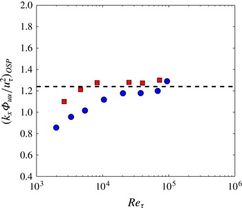
Figure 11. Magnitude of the outer spectral peak: ▪, boundary layer; ●, pipe; – – – – –,
 $k_{x}{\it\Phi}_{uu}/u_{{\it\tau}}^{2}=1.24$
.
$k_{x}{\it\Phi}_{uu}/u_{{\it\tau}}^{2}=1.24$
.
The wavenumber associated with the outer spectral peak,
 $k_{OSP}$
, is shown in figure 12. For increasing Reynolds number, it decreases in viscous units as
$k_{OSP}$
, is shown in figure 12. For increasing Reynolds number, it decreases in viscous units as
 $k_{OSP}^{+}\approx M\mathit{Re}_{{\it\tau}}^{-0.5}$
, while increasing in outer scaling as
$k_{OSP}^{+}\approx M\mathit{Re}_{{\it\tau}}^{-0.5}$
, while increasing in outer scaling as
 $k_{OSP}{\it\delta}\approx M\mathit{Re}_{{\it\tau}}^{0.5}$
, where
$k_{OSP}{\it\delta}\approx M\mathit{Re}_{{\it\tau}}^{0.5}$
, where
 $M=0.2$
. In terms of wavelength, this gives
$M=0.2$
. In terms of wavelength, this gives
 ${\it\lambda}_{OSP}^{+}\approx (M/2{\rm\pi})\mathit{Re}_{{\it\tau}}^{0.5}$
and
${\it\lambda}_{OSP}^{+}\approx (M/2{\rm\pi})\mathit{Re}_{{\it\tau}}^{0.5}$
and
 ${\it\lambda}_{OSP}/{\it\delta}\approx (M/2{\rm\pi})\mathit{Re}_{{\it\tau}}^{-0.5}$
, respectively, suggesting that the wavelength associated with the large energetic scales neither scales with the inner length scale, nor with the outer length scale;
${\it\lambda}_{OSP}/{\it\delta}\approx (M/2{\rm\pi})\mathit{Re}_{{\it\tau}}^{-0.5}$
, respectively, suggesting that the wavelength associated with the large energetic scales neither scales with the inner length scale, nor with the outer length scale;
 ${\it\lambda}_{OSP}$
appears to emerge as an independent length scale. In addition,
${\it\lambda}_{OSP}$
appears to emerge as an independent length scale. In addition,
 ${\it\lambda}_{OSP}\approx (M/2{\rm\pi})({\it\delta}{\it\nu}/u_{{\it\tau}})^{0.5}$
, so that at very large Reynolds numbers
${\it\lambda}_{OSP}\approx (M/2{\rm\pi})({\it\delta}{\it\nu}/u_{{\it\tau}})^{0.5}$
, so that at very large Reynolds numbers
 ${\it\nu}/u_{{\it\tau}}\ll {\it\lambda}_{OSP}\ll {\it\delta}$
.
${\it\nu}/u_{{\it\tau}}\ll {\it\lambda}_{OSP}\ll {\it\delta}$
.

Figure 12. Wavenumber of the outer spectral peak in inner (a) and outer coordinates (b): ▪, boundary layer (uncertainty in
 $k_{OSP}^{+}$
is about
$k_{OSP}^{+}$
is about
 $\pm 50\,\%$
; ▫, boundary layer data from Mathis et al. (Reference Mathis, Hutchins and Marusic2009); (solid line),
$\pm 50\,\%$
; ▫, boundary layer data from Mathis et al. (Reference Mathis, Hutchins and Marusic2009); (solid line),
 $k_{x}^{+}=0.02\mathit{Re}_{{\it\tau}}^{-0.5}$
(a);
$k_{x}^{+}=0.02\mathit{Re}_{{\it\tau}}^{-0.5}$
(a);
 $k_{x}{\it\delta}=0.02\mathit{Re}_{{\it\tau}}^{0.5}$
(b); ♢, predicted wavenumber for
$k_{x}{\it\delta}=0.02\mathit{Re}_{{\it\tau}}^{0.5}$
(b); ♢, predicted wavenumber for
 $\mathit{Re}_{{\it\tau}}=$
650 000.
$\mathit{Re}_{{\it\tau}}=$
650 000.
The wavenumber of the outer spectral peak appears, therefore, to be a new scale representative of the log region. Vassilicos et al. (Reference Vassilicos, Laval, Foucaut and Stanislas2014) recently suggested that for the Townsend–Perry attached eddy model to show the correct behaviour for the integral length scale at high Reynolds number, an additional length scale needs to appear, one that lies between the inner and outer scales. Our current observations are closely aligned with that proposal. In addition, the appearance of a new region described by the length scale
 ${\it\lambda}_{OSP}$
is consistent with the observation of Vallikivi et al. (Reference Vallikivi, Hultmark and Smits2015) who find a log region (in mean and intensity) only after the outer spectral peak has emerged.
${\it\lambda}_{OSP}$
is consistent with the observation of Vallikivi et al. (Reference Vallikivi, Hultmark and Smits2015) who find a log region (in mean and intensity) only after the outer spectral peak has emerged.
Given the consensus in the literature that the outer spectral peak is associated with the SS, there are two potential ways to interpret the above observations. First, we could say that the SS are actually the manifestation of this region in the flow, rather than the largest scales of motion. This would lead to a rather startling implication that at lower Reynolds numbers the SS appear as very large scales (that is,
 ${\it\lambda}_{x}/{\it\delta}\approx 3{-}6$
) due to a lack of scale separation, but at higher Reynolds numbers the length scale of the SS decreases. The length scale associated with the outer spectral peak in an atmospheric boundary layer at
${\it\lambda}_{x}/{\it\delta}\approx 3{-}6$
) due to a lack of scale separation, but at higher Reynolds numbers the length scale of the SS decreases. The length scale associated with the outer spectral peak in an atmospheric boundary layer at
 $\mathit{Re}_{{\it\tau}}\approx 650\,000$
is expected to be
$\mathit{Re}_{{\it\tau}}\approx 650\,000$
is expected to be
 ${\it\lambda}_{x}/{\it\delta}\approx 0.4$
(as inferred from the correlation shown in figure 12), which is much smaller than the scales of the VLSM/SS. This suggests that this first interpretation is too stringent and may not truly represent the data.
${\it\lambda}_{x}/{\it\delta}\approx 0.4$
(as inferred from the correlation shown in figure 12), which is much smaller than the scales of the VLSM/SS. This suggests that this first interpretation is too stringent and may not truly represent the data.
An alternate and perhaps more suitable interpretation is that there is a need to decouple the scale and location of the outer spectral peak from that of the SS/VLSMs. It can be seen from the spectra that, although the OSP appears to move towards the wall and become smaller (in outer scaling) with increasing Reynolds number, there is still significant energy content in larger scales. Therefore, the SS (in boundary layers) and VLSMs (in pipes) continue to be dynamically relevant. This means that the wavelength of the outer spectral peak is in fact a new length scale that emerges in parallel with the VLSMs. The VLSMs start to appear at ‘lower’ Reynolds numbers (say
 $\mathit{Re}_{{\it\tau}}\approx 2000$
), but this new length scale only emerges when there is sufficient scale separation even beyond the one required for the VLSMs (
$\mathit{Re}_{{\it\tau}}\approx 2000$
), but this new length scale only emerges when there is sufficient scale separation even beyond the one required for the VLSMs (
 $\mathit{Re}_{{\it\tau}}>20\,000$
). At these higher Reynolds numbers, the VLSMs represent the plateau region in the spectra (instead of the peak) while the peak itself captures this new inertial length scale.
$\mathit{Re}_{{\it\tau}}>20\,000$
). At these higher Reynolds numbers, the VLSMs represent the plateau region in the spectra (instead of the peak) while the peak itself captures this new inertial length scale.
To show that there is at least some support for this notion at even higher Reynolds numbers, figure 13 reproduces the spectrogram obtained in the neutral atmospheric boundary layer by Mathis et al. (Reference Mathis, Hutchins and Marusic2009), where we see that there may indeed be an outer spectral peak whose location is proportional to
 $\ln \mathit{Re}_{{\it\tau}}$
and whose wavelength (in outer units) follows
$\ln \mathit{Re}_{{\it\tau}}$
and whose wavelength (in outer units) follows
 $\mathit{Re}_{{\it\tau}}^{-0.5}$
. The location and the wavelength of this prediction appears to be consistent with the peak found by Guala, Metzger & McKeon (Reference Guala, Metzger and McKeon2011) in the wall-normal range
$\mathit{Re}_{{\it\tau}}^{-0.5}$
. The location and the wavelength of this prediction appears to be consistent with the peak found by Guala, Metzger & McKeon (Reference Guala, Metzger and McKeon2011) in the wall-normal range
 $y^{+}\approx 1000$
at a wavelength of about
$y^{+}\approx 1000$
at a wavelength of about
 $0.45{\it\delta}$
. Note that these values have been inferred from figure 12 in Guala et al. (Reference Guala, Metzger and McKeon2011) that shows multiple peaks at different wall-normal locations and wavenumbers and the uncertainty in identifying a peak in the spectrogram (in wall-normal location) is stated to be about
$0.45{\it\delta}$
. Note that these values have been inferred from figure 12 in Guala et al. (Reference Guala, Metzger and McKeon2011) that shows multiple peaks at different wall-normal locations and wavenumbers and the uncertainty in identifying a peak in the spectrogram (in wall-normal location) is stated to be about
 $\pm 1000$
wall-units.
$\pm 1000$
wall-units.

Figure 13. Contour plot of the spectra in the atmospheric boundary layer at
 $\mathit{Re}_{{\it\tau}}=650\,000$
, adapted from Mathis et al. (Reference Mathis, Hutchins and Marusic2009):
$\mathit{Re}_{{\it\tau}}=650\,000$
, adapted from Mathis et al. (Reference Mathis, Hutchins and Marusic2009):
 $+$
, location of inner spectral peak; ♦, speculated location of outer spectral peak; (solid lines), trends in the loci of LSM and SS peaks as described in § 3.3.
$+$
, location of inner spectral peak; ♦, speculated location of outer spectral peak; (solid lines), trends in the loci of LSM and SS peaks as described in § 3.3.
As noted earlier, pipe flows behave somewhat differently. Here, we expect that
 ${\it\lambda}_{OSP}/{\it\delta}\propto \mathit{Re}_{{\it\tau}}^{-0.67}$
and
${\it\lambda}_{OSP}/{\it\delta}\propto \mathit{Re}_{{\it\tau}}^{-0.67}$
and
 ${\it\lambda}_{OSP}^{+}\propto \mathit{Re}_{{\it\tau}}^{0.33}$
. Hence, the scale separation between inner and inertial ranges appears slower in pipes than in boundary layers, whereas the separation between outer and inertial scales is faster. The slower approach to the inner limit agrees well with the observation that the appearance of a logarithmic region occurs at a higher value of
${\it\lambda}_{OSP}^{+}\propto \mathit{Re}_{{\it\tau}}^{0.33}$
. Hence, the scale separation between inner and inertial ranges appears slower in pipes than in boundary layers, whereas the separation between outer and inertial scales is faster. The slower approach to the inner limit agrees well with the observation that the appearance of a logarithmic region occurs at a higher value of
 $y^{+}$
in pipes than in boundary layers.
$y^{+}$
in pipes than in boundary layers.
4. The mesolayer
We now draw together the observations on the spectral peaks and the behaviour of the mean velocity and the variances. To this end, contour maps of the premultiplied spectra in the boundary layer and pipe are shown in figures 14 and 15, together with the corresponding mean velocity and variance profiles. We see again that the location of the outer spectral peak given by the correlations of Hutchins & Marusic (Reference Hutchins and Marusic2007) and Mathis et al. (Reference Mathis, Hutchins and Marusic2009) for boundary layers overestimate its Reynolds number dependence. In addition, the location of the outer spectral peak coincides closely with the start of the logarithmic regions in the mean velocity and the variance. The overall behaviour of the spectra in pipe flow is very similar to that in boundary layers, in that the inner spectral peak stays approximately constant in viscous units and the outer spectral peak is identified with the start of the log layer, although it is located at slightly higher values of
 $y^{+}$
in pipes compared with boundary layers.
$y^{+}$
in pipes compared with boundary layers.

Figure 14. Contour plots of spectra in the boundary layer at
 $\mathit{Re}_{{\it\tau}}=5\times 10^{3}$
,
$\mathit{Re}_{{\it\tau}}=5\times 10^{3}$
,
 $20\times 10^{3}$
and
$20\times 10^{3}$
and
 $70\times 10^{3}$
. Lines show trends in the loci of peaks shown in figures 8 and 9; (dashed lines),
$70\times 10^{3}$
. Lines show trends in the loci of peaks shown in figures 8 and 9; (dashed lines),
 $y^{+}=10$
, 50,
$y^{+}=10$
, 50,
 $y_{OSP}^{+}$
,
$y_{OSP}^{+}$
,
 $0.15\mathit{Re}_{{\it\tau}}$
; ●, location of near-wall spectral peak. Location of outer spectral peak: ○, current data;
$0.15\mathit{Re}_{{\it\tau}}$
; ●, location of near-wall spectral peak. Location of outer spectral peak: ○, current data;
 $\times$
, Mathis et al. (Reference Mathis, Hutchins and Marusic2009);
$\times$
, Mathis et al. (Reference Mathis, Hutchins and Marusic2009);
 $+$
, Hutchins & Marusic (Reference Hutchins and Marusic2007).
$+$
, Hutchins & Marusic (Reference Hutchins and Marusic2007).

Figure 15. Contour plots of spectra in the pipe at
 $\mathit{Re}_{{\it\tau}}=5\times 10^{3}$
,
$\mathit{Re}_{{\it\tau}}=5\times 10^{3}$
,
 $20\times 10^{3}$
and
$20\times 10^{3}$
and
 $70\times 10^{3}$
. Lines show trends in the loci of peaks shown in figures 8 and 9; (dashed lines),
$70\times 10^{3}$
. Lines show trends in the loci of peaks shown in figures 8 and 9; (dashed lines),
 $y^{+}=10$
, 67,
$y^{+}=10$
, 67,
 $y_{OSP}^{+}$
,
$y_{OSP}^{+}$
,
 $0.15\mathit{Re}_{{\it\tau}}$
; ●, location of near-wall spectral peak; ○, location of outer spectral peak.
$0.15\mathit{Re}_{{\it\tau}}$
; ●, location of near-wall spectral peak; ○, location of outer spectral peak.
Based on these observations, we first identify regions I and II in figures 14 and 15, where the spectra and the statistics scale with inner variables (corresponding to the linear sublayer and the buffer layer). We also recognize a region IV where the mean velocity and variances follow a log-law, marked approximately at its inner boundary by the location of the outer spectral peak, and at its outer boundary by the point where
 $y/{\it\delta}=0.15$
. In between, there is region III where a Reynolds-number-dependent behaviour can be seen in all parameters, which we identify as the mesolayer.
$y/{\it\delta}=0.15$
. In between, there is region III where a Reynolds-number-dependent behaviour can be seen in all parameters, which we identify as the mesolayer.
The term mesolayer was initially introduced by Long & Chen (Reference Long and Chen1981), but found a clearer expression in the work of Afzal (Reference Afzal1982), Afzal (Reference Afzal1984), Sreenivasan & Sahay (Reference Sreenivasan, Sahay and Panton1997), George & Castillo (Reference George and Castillo1997), Wosnik, Castillo & George (Reference Wosnik, Castillo and George2000) and Wei et al. (Reference Wei, Fife, Klewicki and McMurtry2005). With the exceptions of George & Castillo (Reference George and Castillo1997) and Wosnik et al. (Reference Wosnik, Castillo and George2000), who argued that the mesolayer is a region where energy dissipation scales with
 ${\it\nu}u^{2}/y^{2}$
rather than
${\it\nu}u^{2}/y^{2}$
rather than
 $u^{3}/y$
so that a Reynolds number dependence is retained in the scaled Reynolds stress and mean flow equations, all other studies rely on the presence of an emerging intermediate wall-normal length scale that increases as
$u^{3}/y$
so that a Reynolds number dependence is retained in the scaled Reynolds stress and mean flow equations, all other studies rely on the presence of an emerging intermediate wall-normal length scale that increases as
 $\sqrt{\mathit{Re }_{{\it\tau}}}$
. For example, Afzal (Reference Afzal1982) used asymptotic expansions together with an integrated momentum equation to show the emergence of a mesolayer whose location scales as
$\sqrt{\mathit{Re }_{{\it\tau}}}$
. For example, Afzal (Reference Afzal1982) used asymptotic expansions together with an integrated momentum equation to show the emergence of a mesolayer whose location scales as
 $\sqrt{\mathit{Re }_{{\it\tau}}}$
in pipe flow. Sreenivasan & Sahay (Reference Sreenivasan, Sahay and Panton1997) found that the location of the peak in Reynolds shear stress (
$\sqrt{\mathit{Re }_{{\it\tau}}}$
in pipe flow. Sreenivasan & Sahay (Reference Sreenivasan, Sahay and Panton1997) found that the location of the peak in Reynolds shear stress (
 $\langle -uv\rangle ^{+}$
) scales as
$\langle -uv\rangle ^{+}$
) scales as
 $\sqrt{\mathit{Re }_{{\it\tau}}}$
, and expanded the once integrated form of the momentum equation about this peak to determine the extent of the mesolayer. Finally, Wei et al. (Reference Wei, Fife, Klewicki and McMurtry2005), by examining the mean momentum balance in wall-bounded turbulent flows, identified the mesolayer (layer III in their nomenclature) as a region where there is a balance between turbulent inertia (stress gradients), the viscous force, and either the force due to the pressure gradient in pipes or the mean advection in boundary layers. They identified the extent of the mesolayer, and using the data available at the time verified its outer limit to be
$\sqrt{\mathit{Re }_{{\it\tau}}}$
, and expanded the once integrated form of the momentum equation about this peak to determine the extent of the mesolayer. Finally, Wei et al. (Reference Wei, Fife, Klewicki and McMurtry2005), by examining the mean momentum balance in wall-bounded turbulent flows, identified the mesolayer (layer III in their nomenclature) as a region where there is a balance between turbulent inertia (stress gradients), the viscous force, and either the force due to the pressure gradient in pipes or the mean advection in boundary layers. They identified the extent of the mesolayer, and using the data available at the time verified its outer limit to be
 $O(\sqrt{\mathit{Re }_{{\it\tau}}})$
in all flows. A summary description of the different layers and their extent is given by Klewicki (Reference Klewicki2013b
).
$O(\sqrt{\mathit{Re }_{{\it\tau}}})$
in all flows. A summary description of the different layers and their extent is given by Klewicki (Reference Klewicki2013b
).
The current data show a region akin to the above-mentioned mesolayer for the mean flow, the variances and the spectra, but the bounds are different from those determined in previous studies. In the premultiplied spectra, this is the region for
 $y^{+}>50$
(for the boundary layer) and
$y^{+}>50$
(for the boundary layer) and
 $y^{+}>67$
(for the pipe) where the LSM and VLSM/SS peaks can be identified, with these two peaks competing until the VLSM/SS peak becomes dominant. The energy associated with the VLSM/SS peak increases throughout this mesolayer, and the outer spectral peak acts as the outer bound for this region. It is seen that the location of the outer spectral peak does not appear to follow the
$y^{+}>67$
(for the pipe) where the LSM and VLSM/SS peaks can be identified, with these two peaks competing until the VLSM/SS peak becomes dominant. The energy associated with the VLSM/SS peak increases throughout this mesolayer, and the outer spectral peak acts as the outer bound for this region. It is seen that the location of the outer spectral peak does not appear to follow the
 $\sqrt{\mathit{Re }_{{\it\tau}}}$
scaling proposed for pipes and boundary layers in previous studies. Over the entire range of Reynolds numbers available,
$\sqrt{\mathit{Re }_{{\it\tau}}}$
scaling proposed for pipes and boundary layers in previous studies. Over the entire range of Reynolds numbers available,
 $y_{OSP}^{+}$
appears to follow a much weaker scaling (perhaps as
$y_{OSP}^{+}$
appears to follow a much weaker scaling (perhaps as
 $\ln \mathit{Re}_{{\it\tau}}$
) for both pipes and boundary layers. However, upon further examination, as discussed in the previous section, there appears to be two different trends over the range of Reynolds numbers explored here. For Reynolds numbers up to about 20 000,
$\ln \mathit{Re}_{{\it\tau}}$
) for both pipes and boundary layers. However, upon further examination, as discussed in the previous section, there appears to be two different trends over the range of Reynolds numbers explored here. For Reynolds numbers up to about 20 000,
 $y_{OSP}^{+}\propto \sqrt{\mathit{Re }_{{\it\tau}}}$
, whereas for higher Reynolds numbers,
$y_{OSP}^{+}\propto \sqrt{\mathit{Re }_{{\it\tau}}}$
, whereas for higher Reynolds numbers,
 $y_{OSP}^{+}$
appears to be a constant (to within experimental uncertainty).
$y_{OSP}^{+}$
appears to be a constant (to within experimental uncertainty).
It is important to note that previous analytical studies determined the bounds of the mesolayer based on the peak in Reynolds shear stress and not on the location of the outer spectral peak. In fact, Chin et al. (Reference Chin, Philip, Klewicki, Ooi and Marusic2014) recently calculated the Reynolds shear stress distribution using the mean profiles from Hultmark et al. (Reference Hultmark, Vallikivi, Bailey and Smits2013) and found that the peak in Reynolds shear stress follows
 $\sqrt{\mathit{Re }_{{\it\tau}}}$
scaling. However, this location does not match the location of the outer spectral peak as determined here using the same data. To the best of the authors’ knowledge, there is no particular reason for the two locations to exhibit the same Reynolds number scaling. Up to a certain Reynolds number (say,
$\sqrt{\mathit{Re }_{{\it\tau}}}$
scaling. However, this location does not match the location of the outer spectral peak as determined here using the same data. To the best of the authors’ knowledge, there is no particular reason for the two locations to exhibit the same Reynolds number scaling. Up to a certain Reynolds number (say,
 $\mathit{Re}_{{\it\tau}}\approx 20\,000$
), these two locations appear to be close to each other, or at least within the error bars on our data, and the location of the outer spectral peak can be used as a proxy for the location of the Reynolds shear stress peak. For much higher Reynolds numbers, we need additional data to confirm that this correspondence continues to hold true. Therefore, the mesolayer described in the current work may not be the same as those in the other studies that rely on arguments on the Reynolds shear stress distribution.
$\mathit{Re}_{{\it\tau}}\approx 20\,000$
), these two locations appear to be close to each other, or at least within the error bars on our data, and the location of the outer spectral peak can be used as a proxy for the location of the Reynolds shear stress peak. For much higher Reynolds numbers, we need additional data to confirm that this correspondence continues to hold true. Therefore, the mesolayer described in the current work may not be the same as those in the other studies that rely on arguments on the Reynolds shear stress distribution.
Finally, it is interesting to note that the streamwise length scale, inferred using Taylor’s hypothesis, associated with the outer spectral peak appears as an intermediate length scale that seems to scale with
 $\sqrt{\mathit{Re }_{{\it\tau}}}$
in both pipes and boundary layers. We therefore suggest that the mesolayer may be identified with the emergence of this new streamwise length scale. This observation differs from previous work where the focus was on the emergence of a new wall-normal length scale. Further work is required to understand the emergence of this length scale and how it might be associated with the mesolayer scaling described in other studies.
$\sqrt{\mathit{Re }_{{\it\tau}}}$
in both pipes and boundary layers. We therefore suggest that the mesolayer may be identified with the emergence of this new streamwise length scale. This observation differs from previous work where the focus was on the emergence of a new wall-normal length scale. Further work is required to understand the emergence of this length scale and how it might be associated with the mesolayer scaling described in other studies.
5. The log-layer
For boundary layers and pipes, we saw that at a sufficiently high Reynolds number the location of the outer spectral peak appears to be either fixed or slowly varying in inner scaling, and its magnitude appears to asymptote to a constant value of about
 $1.24\pm 0.05$
(figure 11). The spectrograms shown in figures 14 and 15 demonstrate that the location of the outer spectral peak at high Reynolds numbers marks the start of a broad plateau where, at any given wall-normal location
$1.24\pm 0.05$
(figure 11). The spectrograms shown in figures 14 and 15 demonstrate that the location of the outer spectral peak at high Reynolds numbers marks the start of a broad plateau where, at any given wall-normal location
 $k_{x}{\it\Phi}_{uu}/u_{{\it\tau}}^{2}\approx A_{1}^{\prime }$
, that is,
$k_{x}{\it\Phi}_{uu}/u_{{\it\tau}}^{2}\approx A_{1}^{\prime }$
, that is,
 ${\it\Phi}_{uu}(k_{x}y)/u_{{\it\tau}}^{2}\approx A_{1}^{\prime }/(k_{x}y)$
. At any given Reynolds number, this plateau extends approximately from a low-wavenumber limit given by a fixed value of
${\it\Phi}_{uu}(k_{x}y)/u_{{\it\tau}}^{2}\approx A_{1}^{\prime }/(k_{x}y)$
. At any given Reynolds number, this plateau extends approximately from a low-wavenumber limit given by a fixed value of
 $k_{x}{\it\delta}=F$
to a high-wavenumber limit given by
$k_{x}{\it\delta}=F$
to a high-wavenumber limit given by
 $k_{x}y=0.4$
. Hence, by integrating the spectrum over this plateau we find a very similar result to that given by (1.2), namely,
$k_{x}y=0.4$
. Hence, by integrating the spectrum over this plateau we find a very similar result to that given by (1.2), namely,
 $$\begin{eqnarray}u^{2+}=\frac{1}{u_{{\it\tau}}^{2}}\int _{Fy/{\it\delta}}^{0.4}{\it\Phi}_{uu}(k_{x}y)\text{d}(k_{x}y)=B_{1}^{\prime }-A_{1}^{\prime }\ln \left[\frac{y}{{\it\delta}}\right].\end{eqnarray}$$
The value of
 $A_{1}^{\prime }\approx 1$
, and so it is generally smaller than
$A_{1}^{\prime }\approx 1$
, and so it is generally smaller than
 $A_{1}$
, and it may also be a weak function of
$A_{1}$
, and it may also be a weak function of
 $y/{\it\delta}$
. Nevertheless, we can derive a logarithmic region in the variances with a slope that is close to the asymptotic value of the outer spectral peak, without requiring an overlap region, providing the lower-wavenumber part of the spectrum scales with
$y/{\it\delta}$
. Nevertheless, we can derive a logarithmic region in the variances with a slope that is close to the asymptotic value of the outer spectral peak, without requiring an overlap region, providing the lower-wavenumber part of the spectrum scales with
 ${\it\delta}$
, the higher-wavenumber part scales with
${\it\delta}$
, the higher-wavenumber part scales with
 $y$
, and
$y$
, and
 $A_{1}^{\prime }$
does not depend strongly on
$A_{1}^{\prime }$
does not depend strongly on
 $y/{\it\delta}$
. Note that the integral of the spectrum is likely to be reasonably insensitive to the details of the spectral distribution, so that the underlying physical arguments, especially the attached eddy hypothesis, retain an important role. In this respect, an alternative theoretical approach was recently suggested by Hultmark (Reference Hultmark2012), who showed a logarithmic behaviour in variances without involving spectral arguments and therefore independent of any
$y/{\it\delta}$
. Note that the integral of the spectrum is likely to be reasonably insensitive to the details of the spectral distribution, so that the underlying physical arguments, especially the attached eddy hypothesis, retain an important role. In this respect, an alternative theoretical approach was recently suggested by Hultmark (Reference Hultmark2012), who showed a logarithmic behaviour in variances without involving spectral arguments and therefore independent of any
 $k_{x}^{-1}$
region in the spectrum.
$k_{x}^{-1}$
region in the spectrum.
These observations suggest that the essential condition to observe a logarithmic behaviour in the variances is a plateau region defined by a sufficient scale separation between
 $y_{OSP}^{+}$
and
$y_{OSP}^{+}$
and
 $y/{\it\delta}=0.15$
. However, the extent of the approximate plateau in the spectrum between
$y/{\it\delta}=0.15$
. However, the extent of the approximate plateau in the spectrum between
 $k_{x}{\it\delta}=F$
and
$k_{x}{\it\delta}=F$
and
 $k_{x}y=0.4$
depends upon the wavenumber of the outer spectral peak. Since
$k_{x}y=0.4$
depends upon the wavenumber of the outer spectral peak. Since
 $k_{OSP}{\it\delta}$
increases and
$k_{OSP}{\it\delta}$
increases and
 $k_{OSP}^{+}$
decreases with increasing
$k_{OSP}^{+}$
decreases with increasing
 $\mathit{Re}_{{\it\tau}}$
, we expect that a plateau (whose value is near 1.24) will emerge over a large range of wavenumbers and wall-normal locations at Reynolds numbers where
$\mathit{Re}_{{\it\tau}}$
, we expect that a plateau (whose value is near 1.24) will emerge over a large range of wavenumbers and wall-normal locations at Reynolds numbers where
 ${\it\nu}/u_{{\it\tau}}\ll {\it\lambda}_{OSP}\ll {\it\delta}$
. These conditions are consistent with those necessary to have
${\it\nu}/u_{{\it\tau}}\ll {\it\lambda}_{OSP}\ll {\it\delta}$
. These conditions are consistent with those necessary to have
 ${\it\lambda}_{OSP}$
emerge as a scale representative of the log-layer.
${\it\lambda}_{OSP}$
emerge as a scale representative of the log-layer.
6. Conclusions
Streamwise turbulent spectra for Reynolds numbers in the range
 $2600\lesssim \mathit{Re}_{{\it\tau}}\lesssim 72\,500$
were studied in boundary layer flows, and compared with data at similar Reynolds numbers taken previously in pipe flows. In the high-wavenumber (low-wavelength) region, all spectra in both flows showed an excellent collapse in Kolmogorov scaling with a slope approaching (but not reaching)
$2600\lesssim \mathit{Re}_{{\it\tau}}\lesssim 72\,500$
were studied in boundary layer flows, and compared with data at similar Reynolds numbers taken previously in pipe flows. In the high-wavenumber (low-wavelength) region, all spectra in both flows showed an excellent collapse in Kolmogorov scaling with a slope approaching (but not reaching)
 $k_{x}^{-5/3}$
for increasing wall-normal distance and Reynolds number. This observation is in agreement with the theory of Mydlarski & Warhaft (Reference Mydlarski and Warhaft1996), Gamard & George (Reference Gamard and George2000) and others, on the slow asymptotic behaviour of the exponent toward
$k_{x}^{-5/3}$
for increasing wall-normal distance and Reynolds number. This observation is in agreement with the theory of Mydlarski & Warhaft (Reference Mydlarski and Warhaft1996), Gamard & George (Reference Gamard and George2000) and others, on the slow asymptotic behaviour of the exponent toward
 $-5/3$
.
$-5/3$
.
At intermediate wavelengths, the spectra were found to scale well with
 $y$
, and at large wavelengths the spectra scaled with the outer length scale
$y$
, and at large wavelengths the spectra scaled with the outer length scale
 ${\it\delta}$
. However, in contrast to the predictions by Perry et al. (Reference Perry, Henbest and Chong1986), no region of overlap of these scalings was seen, as first noted by Morrison et al. (Reference Morrison, McKeon, Jiang and Smits2004).
${\it\delta}$
. However, in contrast to the predictions by Perry et al. (Reference Perry, Henbest and Chong1986), no region of overlap of these scalings was seen, as first noted by Morrison et al. (Reference Morrison, McKeon, Jiang and Smits2004).
For boundary layers, the near-wall inner spectral peak in the premultiplied spectrum followed
 $t^{+}\approx 125$
for
$t^{+}\approx 125$
for
 $y^{+}\lesssim 10$
. At
$y^{+}\lesssim 10$
. At
 $y^{+}\approx 10$
, the loci bifurcated so that the LSM peak first followed
$y^{+}\approx 10$
, the loci bifurcated so that the LSM peak first followed
 $k_{x}^{+}\approx 0.005$
and then
$k_{x}^{+}\approx 0.005$
and then
 $k_{x}y\approx 0.4$
, in close agreement with previous findings in pipe flow. After bifurcation, a peak associated with SS emerged, scaling with outer variables and following
$k_{x}y\approx 0.4$
, in close agreement with previous findings in pipe flow. After bifurcation, a peak associated with SS emerged, scaling with outer variables and following
 ${\it\lambda}_{x}^{+}\approx 20(y^{+}\mathit{Re}_{{\it\tau}})^{0.5}$
for
${\it\lambda}_{x}^{+}\approx 20(y^{+}\mathit{Re}_{{\it\tau}})^{0.5}$
for
 $50\lesssim y^{+}\lesssim 0.15\mathit{Re}_{{\it\tau}}$
. Outside the logarithmic layer above
$50\lesssim y^{+}\lesssim 0.15\mathit{Re}_{{\it\tau}}$
. Outside the logarithmic layer above
 $y/{\it\delta}>0.15$
, the peaks associated with SS and LSM merged into one peak located at about
$y/{\it\delta}>0.15$
, the peaks associated with SS and LSM merged into one peak located at about
 ${\it\lambda}_{x}\approx 3{\it\delta}$
. This is in contrast to pipe flows, where the two peaks remain distinct.
${\it\lambda}_{x}\approx 3{\it\delta}$
. This is in contrast to pipe flows, where the two peaks remain distinct.
The location of the outer spectral peak increased as
 $\sqrt{\mathit{Re }_{{\it\tau}}}$
up to a
$\sqrt{\mathit{Re }_{{\it\tau}}}$
up to a
 $\mathit{Re}_{{\it\tau}}\approx 20\,000$
and beyond that the trend was much weaker and seemed to approach a constant value, suggesting that the physical region containing most of the turbulent energy is getting smaller and moving closer to the wall (in physical units).
$\mathit{Re}_{{\it\tau}}\approx 20\,000$
and beyond that the trend was much weaker and seemed to approach a constant value, suggesting that the physical region containing most of the turbulent energy is getting smaller and moving closer to the wall (in physical units).
In boundary layers and pipes, the wavelength of the outer spectral peak appeared to increase with Reynolds number using inner scaling and decrease with Reynolds number using outer scaling, so that the scales associated with the outer spectral peak decrease in size relative to the large scales with increasing Reynolds number. It is possible, therefore, that the wavelength of the outer spectral peak is a representative scale of the inertial range where
 ${\it\nu}/u_{{\it\tau}}\ll {\it\lambda}_{OSP}\ll {\it\delta}$
. At high Reynolds numbers, the location of the outer spectral peak
${\it\nu}/u_{{\it\tau}}\ll {\it\lambda}_{OSP}\ll {\it\delta}$
. At high Reynolds numbers, the location of the outer spectral peak
 $y_{OSP}$
marks the start of a broad plateau in the premultiplied spectrum that gives the appearance of a
$y_{OSP}$
marks the start of a broad plateau in the premultiplied spectrum that gives the appearance of a
 $k_{x}^{-1}$
region. The extent of the plateau depends upon satisfying
$k_{x}^{-1}$
region. The extent of the plateau depends upon satisfying
 ${\it\nu}/u_{{\it\tau}}\ll {\it\lambda}_{OSP}\ll {\it\delta}$
. By integrating the spectrum over the plateau region, we derive a logarithmic region in the variances with a slope that is close to the value of 1.24, as was found to exist in pipes and boundary layers by Hultmark et al. (Reference Hultmark, Vallikivi, Bailey and Smits2012), Hultmark et al. (Reference Hultmark, Vallikivi, Bailey and Smits2013), Marusic et al. (Reference Marusic, Monty, Hultmark and Smits2013) and Vallikivi et al. (Reference Vallikivi, Hultmark and Smits2015). Hence, the log-layer in wall-bounded flows seems directly associated with the appearance of an outer spectral peak whose wall-normal location scales with wall units. For the laboratory results presented here, an extensive
${\it\nu}/u_{{\it\tau}}\ll {\it\lambda}_{OSP}\ll {\it\delta}$
. By integrating the spectrum over the plateau region, we derive a logarithmic region in the variances with a slope that is close to the value of 1.24, as was found to exist in pipes and boundary layers by Hultmark et al. (Reference Hultmark, Vallikivi, Bailey and Smits2012), Hultmark et al. (Reference Hultmark, Vallikivi, Bailey and Smits2013), Marusic et al. (Reference Marusic, Monty, Hultmark and Smits2013) and Vallikivi et al. (Reference Vallikivi, Hultmark and Smits2015). Hence, the log-layer in wall-bounded flows seems directly associated with the appearance of an outer spectral peak whose wall-normal location scales with wall units. For the laboratory results presented here, an extensive
 $k_{x}^{-1}$
range is not obvious due to a lack of sufficient scale separation between inner scales, outer scales and the inertial scale
$k_{x}^{-1}$
range is not obvious due to a lack of sufficient scale separation between inner scales, outer scales and the inertial scale
 ${\it\lambda}_{OSP}$
. This observation, however, is consistent with the presence of
${\it\lambda}_{OSP}$
. This observation, however, is consistent with the presence of
 $k_{x}^{-1}$
in even higher-Reynolds-number flows where this scale separation is present, such as in atmospheric boundary layers.
$k_{x}^{-1}$
in even higher-Reynolds-number flows where this scale separation is present, such as in atmospheric boundary layers.
Based on the behaviour of peaks in the energy spectra, together with the results on the turbulence statistics obtained by Vallikivi et al. (Reference Vallikivi, Hultmark and Smits2015), we now propose five distinct regions in wall-bounded flows:
Region I:
 $y^{+}\lesssim 10$
. Here, the near-wall structures scale as
$y^{+}\lesssim 10$
. Here, the near-wall structures scale as
 ${\it\lambda}_{x}/y\approx \text{const.}$
(or
${\it\lambda}_{x}/y\approx \text{const.}$
(or
 $t^{+}\approx \text{const.}$
without using Taylor hypothesis). The inner spectral peak location corresponds to
$t^{+}\approx \text{const.}$
without using Taylor hypothesis). The inner spectral peak location corresponds to
 $y^{+}\approx 10$
and
$y^{+}\approx 10$
and
 ${\it\lambda}^{+}\approx 1250$
(
${\it\lambda}^{+}\approx 1250$
(
 $k_{x}^{+}=0.005$
), close to the location of the inner peak in the variance.
$k_{x}^{+}=0.005$
), close to the location of the inner peak in the variance.

Figure 16. The extent of the principal scaling regions in boundary layers, in inner (a) and outer coordinates (b).
Region II:
 $10\lesssim y^{+}\lesssim 50$
(boundary layers) and 67 (pipes). Here, the near-wall structures scale as
$10\lesssim y^{+}\lesssim 50$
(boundary layers) and 67 (pipes). Here, the near-wall structures scale as
 ${\it\lambda}_{x}^{+}\approx \text{const}$
. The energy in the near-wall structures decreases and the wavelength of these structures stays about constant in viscous units at
${\it\lambda}_{x}^{+}\approx \text{const}$
. The energy in the near-wall structures decreases and the wavelength of these structures stays about constant in viscous units at
 ${\it\lambda}_{x}^{+}\approx 1250$
. The decrease in the variance with increasing wall distance is matched to the decrease of the near-wall peak in the energy spectra. This region is associated with the buffer layer in the mean velocity.
${\it\lambda}_{x}^{+}\approx 1250$
. The decrease in the variance with increasing wall distance is matched to the decrease of the near-wall peak in the energy spectra. This region is associated with the buffer layer in the mean velocity.
Region III: 50 (boundary layers) and 67 (pipes)
 ${\lesssim}y^{+}\lesssim y_{OSP}^{+}$
. Here,
${\lesssim}y^{+}\lesssim y_{OSP}^{+}$
. Here,
 ${\it\lambda}_{x}^{+}\sim y^{+0.5}\mathit{Re}_{{\it\tau}}^{0.5}$
in boundary layers and
${\it\lambda}_{x}^{+}\sim y^{+0.5}\mathit{Re}_{{\it\tau}}^{0.5}$
in boundary layers and
 ${\it\lambda}_{x}^{+}\sim y^{+2/3}\mathit{Re}_{{\it\tau}}^{1/3}$
in pipes. Two energetic peaks in the spectra are present, with most of the energy associated with the SS located at
${\it\lambda}_{x}^{+}\sim y^{+2/3}\mathit{Re}_{{\it\tau}}^{1/3}$
in pipes. Two energetic peaks in the spectra are present, with most of the energy associated with the SS located at
 ${\it\lambda}_{x}\sim (y{\it\delta})^{0.5}$
, and a weaker peak associated with LSMs located at about
${\it\lambda}_{x}\sim (y{\it\delta})^{0.5}$
, and a weaker peak associated with LSMs located at about
 ${\it\lambda}_{x}\approx 20y$
. The SS/VLSM peak continues to increase until
${\it\lambda}_{x}\approx 20y$
. The SS/VLSM peak continues to increase until
 $y_{OSP}^{+}$
(whose limits are discussed in region IV). The variance is almost constant at lower Reynolds numbers while slightly rising at higher Reynolds numbers. In the mean velocity, the profile seems to behave as a power law in
$y_{OSP}^{+}$
(whose limits are discussed in region IV). The variance is almost constant at lower Reynolds numbers while slightly rising at higher Reynolds numbers. In the mean velocity, the profile seems to behave as a power law in
 $y^{+}$
. This region is associated with the mesolayer, where the mean flow is almost free of viscous effects but turbulent quantities are still affected by viscosity.
$y^{+}$
. This region is associated with the mesolayer, where the mean flow is almost free of viscous effects but turbulent quantities are still affected by viscosity.
Region IV:
 $y_{OSP}^{+}\lesssim y^{+}\lesssim 0.15\mathit{Re}_{{\it\tau}}$
. Here,
$y_{OSP}^{+}\lesssim y^{+}\lesssim 0.15\mathit{Re}_{{\it\tau}}$
. Here,
 ${\it\lambda}_{x}^{+}\sim y^{+0.5}\mathit{Re}_{{\it\tau}}^{0.5}$
in boundary layers and
${\it\lambda}_{x}^{+}\sim y^{+0.5}\mathit{Re}_{{\it\tau}}^{0.5}$
in boundary layers and
 ${\it\lambda}_{x}^{+}\sim y^{+2/3}\mathit{Re}_{{\it\tau}}^{1/3}$
in pipes. The energy associated with the SS/VLSMs is decreasing and there is a logarithmic behaviour in variances. The outer spectral peak associated with SS is located where there is an outer peak in the variance. Also,
${\it\lambda}_{x}^{+}\sim y^{+2/3}\mathit{Re}_{{\it\tau}}^{1/3}$
in pipes. The energy associated with the SS/VLSMs is decreasing and there is a logarithmic behaviour in variances. The outer spectral peak associated with SS is located where there is an outer peak in the variance. Also,
 $y_{OSP}^{+}$
varies weakly with increasing Reynolds number (possibly following a
$y_{OSP}^{+}$
varies weakly with increasing Reynolds number (possibly following a
 $\ln \mathit{Re}_{{\it\tau}}$
trend over the entire range of
$\ln \mathit{Re}_{{\it\tau}}$
trend over the entire range of
 $\mathit{Re}_{{\it\tau}}$
), contrary to previous work that indicated a stronger Reynolds number dependence (over a smaller range of Reynolds numbers). In fact, as discussed in the paper,
$\mathit{Re}_{{\it\tau}}$
), contrary to previous work that indicated a stronger Reynolds number dependence (over a smaller range of Reynolds numbers). In fact, as discussed in the paper,
 $y_{OSP}^{+}$
appears to vary as
$y_{OSP}^{+}$
appears to vary as
 $\sqrt{\mathit{Re }_{{\it\tau}}}$
up to
$\sqrt{\mathit{Re }_{{\it\tau}}}$
up to
 $\mathit{Re}_{{\it\tau}}\approx 20\,000$
and then is nearly a constant for higher Reynolds numbers. Its location coincides with the outer peak or the end of plateau seen in the variances, and therefore marks approximately the beginning of the logarithmic behaviour in the variances. The wavelength of the outer spectral peak emerges as a possible length scale for this region. The magnitude of OSP reaches a constant value, and so marks the start of a
$\mathit{Re}_{{\it\tau}}\approx 20\,000$
and then is nearly a constant for higher Reynolds numbers. Its location coincides with the outer peak or the end of plateau seen in the variances, and therefore marks approximately the beginning of the logarithmic behaviour in the variances. The wavelength of the outer spectral peak emerges as a possible length scale for this region. The magnitude of OSP reaches a constant value, and so marks the start of a
 $k_{x}^{-1}$
plateau that translates to a logarithmic region in the variances.
$k_{x}^{-1}$
plateau that translates to a logarithmic region in the variances.
Region V:
 $y/{\it\delta}\gtrsim 0.15$
. Here, the LSMs (and VLSMs in pipe) scale with the outer length scale. In boundary layers, the SS peak disappears, and only the LSM peak remains, showing up as a single peak associated with large-scale structures with
$y/{\it\delta}\gtrsim 0.15$
. Here, the LSMs (and VLSMs in pipe) scale with the outer length scale. In boundary layers, the SS peak disappears, and only the LSM peak remains, showing up as a single peak associated with large-scale structures with
 ${\it\lambda}_{x}\approx 3{\it\delta}$
. In pipe flows, both the LSM and VLSM peaks continue to be present, scaling on
${\it\lambda}_{x}\approx 3{\it\delta}$
. In pipe flows, both the LSM and VLSM peaks continue to be present, scaling on
 ${\it\delta}$
and differing only in length. The turbulent fluctuations diminish and the mean velocity follows a Reynolds-number\_independent wake function.
${\it\delta}$
and differing only in length. The turbulent fluctuations diminish and the mean velocity follows a Reynolds-number\_independent wake function.
The extent of these regions with varying Reynolds number is illustrated in figure 16. It is clear that regions IV and V will constitute almost the full physical extent of wall-bounded flows at very high Reynolds number.
Acknowledgements
The authors would to thank W. K. George and I. Marusic for insightful discussions and suggestions, and J. Klewicki for some very helpful observations. This work was made possible by support received through ONR grant N00014-13-1-0174, program manager R. Joslin, and NSF grant CBET-1064257, managers H. Winter and D. Papavassiliou. B.G. acknowledges the support from the European Research Council under the European Union’s Seventh Framework Programme (FP7/2007-2013), ERC grant agreement no. 277472.


