


1. Introduction
From breaking waves (Deane & Stokes Reference Deane and Stokes2002) and free surface turbulence (Yu, Hendrickson & Yue Reference Yu, Hendrickson and Yue2020) to chemical and nuclear reactors (Michiyoshi & Serizawa Reference Michiyoshi and Serizawa1986; Jakobsen Reference Jakobsen2008), two-phase flows consisting of finite-sized deformable bubbles or droplets are ubiquitous in nature and industrial applications. Their complicated interaction with the surrounding turbulent flows poses significant challenges to both numerical and experimental methods (Verschoof et al. Reference Verschoof, Van Der Veen, Sun and Lohse2016; Loisy & Naso Reference Loisy and Naso2017; Alméras et al. Reference Alméras, Mathai, Sun and Lohse2019; Du Cluzeau, Bois & Toutant Reference Du Cluzeau, Bois and Toutant2019), as the interface deformation tends to modulate many hydrodynamic forces experienced by bubbles/droplets. In particular, it is well known that additional fluid forces tend to act upon an object as it accelerates relative to its surrounding flow; in turbulence, however, this relative acceleration between the two phases could originate either from the unsteady turbulent background flow or bubble/droplet deformation.
To understand the added-mass force, consider a case of fluid suddenly exerting force  $\boldsymbol {F}$ on a neutrally buoyant object in translational motion without rotation (Batchelor Reference Batchelor1967). By applying the potential flow theory, this force can be expressed as a function of the velocity potential (
 $\phi$):
  $\boldsymbol {F}=-\rho _l \int (\partial \phi /\partial t) \hat {\boldsymbol {n}} \,\textrm {d}A$, where
  $\rho _l$ is the density of the ambient fluid. Since the velocity potential can be expressed as
  $\partial \phi /\partial t=\dot {\boldsymbol {u}}_s\cdot \pmb {\varPhi }$, this unsteady force can be written as
  $F_i=-\rho _l (a_{s})_j\int \varPhi _jn_i\,\textrm {d}A$, where
  $\pmb {\varPhi }$ solely depends on the object's shape. Because the force
  $F_i$ is linearly proportional to the object slip acceleration
  $(a_{s})_j$ based on Newton's second law, the remaining coefficient (
 $\boldsymbol {A}_{ij}= \rho _l\int \varPhi _jn_i\,\textrm {d}A$) can be treated as an induced or virtual mass, which must be added to the real mass of the object when determining its response to a given applied force. The added-mass tensor
  $\boldsymbol {A}$ can be written as
  $\rho _l V_b\boldsymbol {C}_A$, where
  $\rho _l V_b$ is the mass of the object if filled with outside liquid with density
  $\rho _l$ and
  $\boldsymbol {C}_A$ is the tensorial added-mass coefficient. In addition to the added mass in response to translational acceleration, the potential flow analysis can also be extended to describe an object's response to a sudden torque from the surrounding fluid. In this case, the virtual moment of inertia (
 $\boldsymbol {D}$) must be added to the object's own moment of inertia (
 $\boldsymbol {J}$) when calculating the resulting object's angular acceleration (Lamb Reference Lamb1924; Brennen Reference Brennen1982).
For objects moving in unsteady flows with non-negligible viscous effects, in addition to the added mass (moment of inertia), the vorticity generated on the body surface and its subsequent diffusion and advection into the surrounding flow could also be important (Howe Reference Howe1995). To understand whether the added-mass coefficient will deviate from the potential flow calculation due to the viscous effect, extensive investigations have been attempted to quantify the  $C_A$ of a spherical solid particle (Mei, Lawrence & Adrian Reference Mei, Lawrence and Adrian1991) and bubble (Mei & Klausner Reference Mei and Klausner1992) in flows with small-amplitude oscillations, as well as a rigid spherical particle in an oscillatory (Chang & Maxey Reference Chang and Maxey1994) and constantly accelerated flow (Chang & Maxey Reference Chang and Maxey1995). These results all indicated that the added-mass coefficient (
 $C_A$) of a sphere is 0.5, independent of the particle Reynolds number, Strouhal number and, more importantly, the slip (clean gas bubbles) and no-slip (rigid spheres) boundary conditions. Note that finding that the added-mass force is independent of the object surface boundary condition allows separating the hydrodynamic effects due to vorticity from those described by the irrotational flow theory. The added-mass coefficient of objects with arbitrary shapes calculated from the irrotational potential flow theory (Lamb Reference Lamb1924) can therefore be directly applied to bubbles moving in turbulence with finite Reynolds numbers.
After separating the added-mass force from other hydrodynamic forces that may depend on the particle Reynolds number, the equation of particle motion, including both the translational and rotational components, can be expressed following the generalized Kelvin–Kirchhoff equations (Lamb Reference Lamb1924; Howe Reference Howe1995),
 \begin{gather} (m_b\boldsymbol{I} + \boldsymbol{A})\boldsymbol{a}_s + \boldsymbol{\varOmega} \times ((m_b\boldsymbol{I} + \boldsymbol{A})\boldsymbol{u}_s) = \boldsymbol{F} + (m_b - \rho_lV_b)\boldsymbol{g}, \end{gather}
 \begin{gather}(\boldsymbol{J} + \boldsymbol{D})\boldsymbol{a}_s + \boldsymbol{\varOmega} \times ((\boldsymbol{J} + \boldsymbol{D})\boldsymbol{\varOmega}) + \boldsymbol{u}_s\times (\boldsymbol{A}\boldsymbol{u}_s) = \boldsymbol{\varGamma}, \end{gather}
where  $\pmb {\varOmega }$ is the instantaneous angular velocity of the bubble,
  $\boldsymbol {I}$ and
  $\boldsymbol {J}$ are the unit tensor and inertia tensor of the object, respectively. Here
  $\boldsymbol {F}$ and
  $\boldsymbol {\varGamma }$ are the force and torque arising from the surrounding flow. For an oblate spheroid, the added-mass tensor
  $\boldsymbol {A}$ and added moment of inertia tensor
  $\boldsymbol {D}$ are diagonal if they are in the body-axis frame along the particle's axis of symmetry. The last term on the right-hand side of (1.1a) accounts for the buoyancy force with
  $\boldsymbol {g}$ being the gravitational constant. Here, (1.1a) and (1.1b) are fully coupled to determine the translational and rotational momentum balance of a particle. They have to be solved simultaneously along with the Navier–Stokes equation for the surrounding fluid to determine the bubble motion.
This framework can be used to understand the non-rectilinear path of a bubble rising in an otherwise quiescent medium (Mougin & Magnaudet Reference Mougin and Magnaudet2006; Cano-Lozano et al. Reference Cano-Lozano, Martinez-Bazan, Magnaudet and Tchoufag2016; Mathai, Lohse & Sun Reference Mathai, Lohse and Sun2020). A finite-sized bubble rising in a fluid at rest typically begins with a straight vertical path which develops into a two-dimensional zigzag motion followed by a spiral circular trajectory. Such a non-rectilinear motion of bubbles results from the balance between the wake-induced hydrodynamic loads (forces and torques) and the added-mass effects (Fernandes et al. Reference Fernandes, Ern, Risso and Magnaudet2008). Mougin & Magnaudet (Reference Mougin and Magnaudet2006) utilized the generalized Kevin–Kirchhoff equation to extract the contributions of different forces acting on a freely rising spheroidal bubble with a fixed shape. The added-mass force is important for both zigzag and helix motions. During zigzag motions, the translational added-mass force along the vertical direction is approximately 13 % of the buoyancy force. For the helix motion, along the lateral direction, the centripetal added mass ( $\boldsymbol {\varOmega } \times ( \boldsymbol {A}\boldsymbol {u}_s)$) balances the bubble acceleration in the direction normal to the bubble trajectory, while the transverse added-mass force opposes the sum of the bubble lateral velocity change and the buoyancy force projected to the lateral direction. These findings show that the added-mass force is essential to the non-rectilinear motion of bubbles rising in an otherwise quiescent aqueous medium.
Evaluating the added-mass force experimentally is quite challenging and it was often conducted with the assistance of simulation. De Vries, Luther & Lohse (Reference De Vries, Luther and Lohse2002) experimentally investigated an induced oscillation of a bubble, after being tripped by a wire, while rising in quiescent water. This work showed that, without the added-mass effects, the observed bubble path oscillations could not be reproduced through calculations. Furthermore, Lavrenteva, Prakash & Nir (Reference Lavrenteva, Prakash and Nir2016) studied the interaction of air bubbles in low-Reynolds-number Taylor–Couette flows and demonstrated that the added-mass force is key to explaining the observed separation of neighbouring bubbles (Prakash et al. Reference Prakash, Lavrenteva, Byk and Nir2013).
Although these works clearly articulated the importance of the added-mass force for bubbles, it remains elusive how to prescribe a correct added-mass tensor for a deformable bubble subjected to intense turbulent acceleration where the deformation and bubble orientation are strongly coupled with the surrounding flow. In the current work, we intend to use simultaneous measurements of both bubbles and surrounding turbulence to constrain the added-mass tensor of deforming bubbles in intense turbulence. In § 2, we briefly introduce the experimental set-up and discuss the quantities needed to constrain the added-mass tensor  $\boldsymbol {A}$ experimentally. The analytical solutions for rigid geometries such as spheres, spheroids and cylinders are discussed in appendix A, which are later used to verify whether they can be directly applied to determine the added-mass effects experienced by deformable bubbles, whose shapes and orientations are coupled with turbulence. The procedure to estimate the added mass, including a constant
  $C_A$ (§ 3.2) and the full tensorial form
  $\boldsymbol {C}_A$ (§ 3.3) and how they depend on the bubble shape and orientation in turbulence is introduced in § 3. Section 4 summarizes the paper and presents suggestions for future research.
2. Experimental methods
2.1. Experimental facility
Experiments were conducted in a vertical, 2.7-metre-tall water tunnel named V-ONSET (Masuk et al. Reference Masuk, Salibindla, Tan and Ni2019b), which was specifically designed and built to study the interaction of deformable air bubbles with intense turbulence. Nearly homogeneous and isotropic turbulence (known as HIT) was maintained in this set-up via randomized high-speed jets with speeds reaching up to  $12\ \textrm {m}\ \textrm {s}^{-1}$, which were driven by a pressurized water tank connected to a 3-D-printed device, i.e. the jet array. This array consists of 88 jet nozzles, each of which is controlled by a dedicated solenoid valve, and the array sits atop an octagonal test section with a shape designed to provide flat optical windows covering the tunnel's perimeter. The mean turbulence energy dissipation rate in the measurement section was approximately
  $\langle \epsilon \rangle = 0.5\ \textrm {m}^{2}\ \textrm {s}^{-3}$, with a Taylor-scale Reynolds number of
  $Re_\lambda = 346$.
Bubbles were injected from the bottom of the test section through a bubble bank consisting of four islands of capillary needles with two different sizes. Most bubbles in the test section were around 2–7 mm in diameter, with the majority around 3–4 mm. This bubble size roughly ranges from 40 $\eta$ to 140
 $\eta$ (
 $\eta$ is the Kolmogorov scale), which falls within the inertial range of turbulence. The injected bubbles slowly rise to the centre of the test section, where they encounter turbulence. To extend the residence time of bubbles in the interrogation volume, a downward mean flow was set at around
  $25 \ \textrm {cm}\ \textrm {s}^{-1}$ to slow the bubble rise velocity. Additional set-up details and turbulence characteristics can be found in Masuk et al. (Reference Masuk, Salibindla, Tan and Ni2019b).
The data acquisition system consists of six high-speed cameras that can capture images at 4000 frames per second at their full resolution of one megapixel. These six cameras were strategically placed around the centre of the measurement section in order to optimize the three-dimensional reconstruction of the bubble geometry. Furthermore, the water phase was seeded with density-matched tracer particles in order to visualize the flows around bubbles. Each camera has a dedicated light panel that casts the shadows of bubbles and surrounding tracer particles onto the cameras’ imaging plane, and the two phases were segmented from images based on their size and contrast. The silhouettes of bubbles from all six cameras were combined using a recently developed virtual-camera visual hull method (Masuk, Salibindla & Ni Reference Masuk, Salibindla and Ni2019a) to reconstruct their geometries. The tracer particles were processed through another in-house particle tracking code (Tan et al. Reference Tan, Salibindla, Masuk and Ni2019, Reference Tan, Salibindla, Masuk and Ni2020) to analyse a high concentration of tracer particles around each bubble. In total, we collected approximately 6942 bubble trajectories with 30–40 tracer particles surrounding each bubble. These data sets will be used to extract the statistics of the bubble acceleration and the added-mass force.
2.2. Summary of measurable quantities
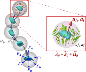
This section summarizes the physical quantities measured through our experiments. Figure 1 shows an example bubble trajectory approximately 400 frames in length, where the reconstructed bubble geometries are plotted once every one hundred frames along the trajectory. The geometry can be used to acquire the bubble size ( $D$), aspect ratio (
 $\chi =r_1/r_3$) and the orientation of both semi-major (
 $\hat {\boldsymbol {r}}_1$) and semi-minor (
 $\hat {\boldsymbol {r}}_3$) axes. Moreover, the three-dimensional locations of surface points on the reconstructed geometry can be averaged to obtain the centre of mass of the bubble, which was tracked over time to construct the bubble trajectory.

Figure 1. Reconstructed three-dimensional trajectory of a bubble ( $D=5.1$ mm) over 0.1 s (400 frames). The three dimensional (3-D) bubble geometries are shown every hundred frames as green blobs. The grey arrows protruding from the centre of these blobs represent the instantaneous bubble velocities. A sphere around each bubble represents a search volume that is used to seek tracer particles, whose locations for one time instant are marked as yellow dots. Their velocity
  $\boldsymbol {u}^p_l$ are indicated in the zoomed-in picture. The blue arrows on one bubble represent all the relevant forces experienced by the bubble.
To obtain the bubble velocity ( $\boldsymbol {u}_b$) and acceleration (
 $\boldsymbol {a}_b$) along their trajectories, each bubble track is then convoluted with a Gaussian kernel (Mordant, Crawford & Bodenschatz Reference Mordant, Crawford and Bodenschatz2004), which acts as a low-pass filter that reduces the positional uncertainties to allow accurately estimating velocity and acceleration. The acceleration standard deviation is sensitive to noise and the selected filter length, and we follow the procedure introduced by Voth et al. (Reference Voth, La Porta, Crawford, Alexander and Bodenschatz2002) to justify the filter length used. In figure 2(a), the standard deviation of the bubble acceleration
  $\sqrt {\langle a_b^2 \rangle }$ in the horizontal (
 $x$) direction is shown as a function of the temporal filter width (
 $\tau$) normalized by the Kolmogorov time scale,
  $\tau _\eta = 1.4$ ms. The initial sharp decay of
  $\sqrt {\langle a_b^2 \rangle }$ is due to the noise removal, while the later gradual change is due to the signal being smoothed. These results are consistent with previous findings (Voth et al. Reference Voth, La Porta, Crawford, Alexander and Bodenschatz2002; Ni, Huang & Xia Reference Ni, Huang and Xia2012). A correct filter length can be obtained by fitting the data with a superposition of a power law and an exponential function to account for the fast and slow decays, respectively. The fit is shown as a solid line, while the contribution of the exponential term alone is shown as a dashed line. The vertical intercept of the dashed line at
  $\tau /\tau _\eta =0$ provides the best estimate of the acceleration standard deviation. Based on this value, the filter length of
  $\tau /\tau _\eta = 0.58$ was consistently used to smooth the bubble trajectories.

Figure 2. (a) The standard deviation of the bubble and flow acceleration versus the filter length. For a description of the solid lines and the dashed lines, please see the text below. (b) The distribution of the normalized bubble and tracer accelerations in the horizontal direction using a fixed filter width of  $\tau = 0.58 \tau _\eta$. The dashed line represents a Gaussian function with the same variance as the corresponding data.
The same procedure can be repeated to calculate the tracer velocity ( $\boldsymbol {u}^p_l$) and acceleration (
 $\boldsymbol {a}^p_l$), where the superscript
  $p$ represents individual tracer particles to distinguish them from the locally averaged fluid properties that will be introduced later. In figure 2(a), the same filter-length test has also been performed for tracer particles, and the results are very close to bubbles. Therefore, the same filter length was adopted for both phases. Finally, figure 2(b) shows the probability density functions (p.d.f.) for
  $\boldsymbol {a}_b$ and
  $\boldsymbol {a}^p_l$ in two different directions, which both exhibit a stretched exponential shape that is consistent with previous works (Voth et al. Reference Voth, La Porta, Crawford, Alexander and Bodenschatz2002; Volk et al. Reference Volk, Calzavarini, Verhille, Lohse, Mordant, Pinton and Toschi2008; Prakash et al. Reference Prakash, Tagawa, Calzavarini, Mercado, Toschi, Lohse and Sun2012). The acceleration p.d.f.s of both finite-sized bubbles and small tracer particles are surprisingly close to each other, which may be due to some competing effects. As shown by Qureshi et al. (Reference Qureshi, Bourgoin, Baudet, Cartellier and Gagne2007) and Brown, Warhaft & Voth (Reference Brown, Warhaft and Voth2009), for finite-sized neutrally buoyant particles, although the acceleration p.d.f. shape changes little (except at tails Volk et al. (Reference Volk, Calzavarini, Leveque and Pinton2011)) with finite size effects, the acceleration variance should decrease as the particle size increases. On the other hand, small microbubbles with a significant density difference but no finite-size effect seem to experience large acceleration variance in turbulence (Volk et al. Reference Volk, Calzavarini, Verhille, Lohse, Mordant, Pinton and Toschi2008; Mathai et al. Reference Mathai, Calzavarini, Brons, Sun and Lohse2016). These two competing effects may neutralize each other, resulting in finite-sized bubbles and tracers sharing similar acceleration p.d.f.s.
Figure 1 illustrates that, at each time instant along a bubble trajectory, a search volume (grey semitransparent sphere) of radius  $D_s/2$ (
 $D_s=4D$, where
  $D$ is the equivalent bubble diameter) is used to seek tracer particles with velocity
  $\boldsymbol {u}^p_l$ in the vicinity of a bubble with its centre of mass at location
  $\boldsymbol {x}_{\boldsymbol {0}}$. Applying the Taylor expansion allows decomposition of the flow field within this range into leading terms:
  $\boldsymbol {u}_l(\boldsymbol {x}_{\boldsymbol {0}})$ and
  $\tilde {{\mathsf{A}}}_{{\mathsf{ij}}}x^p_j$, where
  $\boldsymbol {u}_l=\sum ^{n}_{p=1} \boldsymbol {u}^p_l(\boldsymbol {x}_{\boldsymbol {0}}+\boldsymbol {x}^p)/N$ is the local mean flow averaged over
  $N$ selected tracer particles. This procedure can be repeated to calculate the average flow acceleration
  $\boldsymbol {a}_l = \sum ^{n}_{p=1} \boldsymbol {a}^p_l(\boldsymbol {x}_{\boldsymbol {0}}+\boldsymbol {x}^p)/N$. Here
  $\tilde {{\mathsf{A}}}_{{\mathsf{ij}}}$ is the velocity gradient tensor around the bubble, and the tilde indicates that this gradient is coarse grained at the bubble size. The symmetrical component of
  $\tilde {{\mathsf{A}}}_{{\mathsf{ij}}}$ is the coarse-grained strain-rate tensor,
  $\tilde {{\mathsf{S}}}_{{\mathsf{ij}}}$. In addition,
  $\boldsymbol {x}^p$ is the separation vector directed from the bubble centre at
  $\boldsymbol {x}_{\boldsymbol {0}}$ to the
  $p^{th}$ tracer particle. Here
  $\tilde {{\mathsf{A}}}_{{\mathsf{ij}}}$ can be solved if there are four particles around a bubble. On average, 30–40 particles were used to perform least squares fits by seeking the minimum value of the squared residuals
  $\sum _p[u^p_i-\tilde {{\mathsf{A}}}_{{\mathsf{ij}}}x^p_j]^2$ (Pumir, Bodenschatz & Xu Reference Pumir, Bodenschatz and Xu2013; Ni et al. Reference Ni, Kramel, Ouellette and Voth2015). Several enforced criteria ensure that only the results with reliable
  $\tilde {{\mathsf{A}}}_{{\mathsf{ij}}}$ will be included in the statistics (Masuk, Salibindla & Ni Reference Masuk, Salibindla and Ni2020b). Due to the limited particle concentration, applying a search diameter of
  $D_s$ tends to underestimate
  $\tilde {{\mathsf{A}}}_{{\mathsf{ij}}}$ around a bubble with size
  $D$ due to the larger filter effect (
 $D_s>D$). Because both
  $D_s$ and
  $D$ fall in the inertial range, assuming a constant local energy dissipation rate enables correcting
  $\tilde {{\mathsf{A}}}_{{\mathsf{ij}}}$ with a factor of
  $(D_s/D)^{2/3}$ to account for the scale difference. Additional details using different
  $D_s$ to confirm this correction have been reported by Masuk et al. (Reference Masuk, Salibindla and Ni2020b).
3. Results and discussion
3.1. Governing equation
To determine the motion of a deformable bubble in turbulence rigorously using the generalized Kelvin–Kirchhoff equation (1.1), the force ( $\boldsymbol {F}$) and torque (
 $\boldsymbol {\varGamma }$) from the surrounding flow should be calculated by integrating the hydrodynamic stresses over the entire bubble surface at each time instant along its trajectory. This calculation remains impractical, however, due to the challenges of measuring the full three-dimensional flow velocity very close to the bubble surface at a sufficiently high resolution. Instead of directly measuring the total force, this paper expands the force on the right-hand side of (1.1a) by following the formulation provided by Magnaudet & Eames (Reference Magnaudet and Eames2000) for spherical bubbles under the point-particle assumption, without considering the contribution of rotation. Furthermore, the original equation is adapted for deformable non-spherical bubbles by maintaining the tensorial form of the added-mass coefficient,
 \begin{align} V_{b} \rho_{b} \frac{\textrm{d} \boldsymbol{u}_{b}}{\textrm{d} t}&= \rho_{l} V_{b} \boldsymbol{C}_{A}\left(\frac{{\rm D} \boldsymbol{u}_{l}}{{\rm D} t}-\frac{\textrm{d} \boldsymbol{u}_{b}}{\textrm{d} t}\right) + \frac{\rho_l}{2}A_b C_D(\boldsymbol{u}_l-\boldsymbol{u}_b)|\boldsymbol{u}_l- \boldsymbol{u}_b| - V_b \boldsymbol{\nabla} P_w + \boldsymbol{F}_h \nonumber\\ &\quad + \rho_l C_L(\boldsymbol{u}_l-\boldsymbol{u}_b)\times (\boldsymbol{\nabla} \times \boldsymbol{u}_l) + V_b(\rho_l-\rho_b)g\boldsymbol{\hat{e}}_z, \end{align}
where  $\textrm {d}/\textrm {d}t$ and
  $\textrm {D}/\textrm {D}t$ represent the material derivative along the bubble and tracer Lagrangian trajectories, respectively. The five terms on the right-hand side of (3.1) represent the drag (
 $F_{D}$), pressure (
 $F_{P}$), history (
 $F_{h}$), lift (
 $F_{L}$) and the buoyancy (
 $F_{G}$) forces, respectively. Here,
  $\boldsymbol {\nabla } P_w$ is the pressure gradient of flows around the bubble,
  $\boldsymbol {u}_l$ is the velocity of the unperturbed ambient flow taken at the centre of the bubble if the bubble were absent, and
  $\boldsymbol {u}_s = \boldsymbol {u}_b - \boldsymbol {u}_l$ is the bubble slip velocity. The equation also contains other constants, including the gravitational constant
  $g$ and the density of water and gas, i.e.
  $\rho _l$ and
  $\rho _b$. Here
  $V_b$ is the bubble volume and
  $A_b$ is the projected area of a volume-equivalent sphere. In addition,
  $C_D$ and
  $C_L$ are the drag and lift coefficients, respectively, and
  $\boldsymbol {C}_A$ is the added-mass coefficient tensor. In the previous work by Salibindla et al. (Reference Salibindla, Masuk, Tan and Ni2020), the
  $C_D$ and
  $C_L$ for bubbles with contaminated interfaces in intense turbulent environments were determined based on the mean bubble and flow velocities, and they are
 \begin{gather} C_D = {\text{max}}(24/Re_b(1+0.15Re_b^{0.687}),{\text{min}}(f(Eo), f(Eo)/We^{1/3})), \end{gather}
 \begin{gather}C_L = \begin{cases} 2.671We^{3/5} & We < 0.1, \\ 1.25 - 1.608 We^{3/5} & 0.1 < We < 0.9,\\ -0.23 & 0.9 < We, \end{cases} , \end{gather}
where  $f(Eo) = 8Eo/3(Eo+4)$ is a function of the Eötvös number, i.e.
  $Eo=(\rho _l-\rho _b) g D^2 /\sigma$. The bubble Reynolds number and Weber number are defined as
  $Re_b= |u_b - u_l|D/\nu _l$ and
  $We=2.13\rho (\epsilon D)^{2/3}D/\sigma$, respectively (2.13 is the Kolmogorov constant for the second-order longitudinal structure function). Here
  $We$ determines the turbulence-induced deformation. The bubble size (
 $D$) was determined from the three-dimensional shape reconstruction for each time instant along a bubble trajectory, and instantaneous local flows and bubble velocity were used to calculate
  $Re_b$ and
  $We$. The local Weber number is determined using
  $We={\rho (\widetilde {\lambda _3}D)^2D}/{\sigma }$, where
  $\widetilde {\lambda _3}$ is the smallest eigenvalue of the coarse-grained velocity gradient tensor (
 $\tilde {{\mathsf{A}}}_{{\mathsf{ij}}}$) calculated around each bubble. As shown in a previous work by Masuk et al. (Reference Masuk, Salibindla and Ni2020b), this provides a reliable method to evaluate the instantaneous
  $We$. These dimensionless numbers were then substituted in (3.2) and (3.3) to determine the instantaneous drag and lift coefficients, respectively.
Equation (3.1) ignores the contribution from the bubble rotation. For a deformable bubble moving through water, two mechanisms enable bubbles to reorient: rotation or deformation. In a quiescent medium, bubbles can reorient via rotation driven by the unbalanced-wake-induced force. For finite-sized bubbles deforming in intense turbulence, the reorientation was found to be dominated by deformation along a different direction (Masuk et al. Reference Masuk, Qi, Salibindla and Ni2020a). Therefore, in accordance to this recent finding, the rotation of the bubble ( $\boldsymbol {\varOmega }$) throughout the rest of this paper is assumed to be zero. As a result, the hydrodynamic torque, the added moment of inertia and corresponding equation (1.1b) are ignored for simplification.
After replacing the slip acceleration and the added-mass tensor  $\boldsymbol {A}$ with
  $\boldsymbol {a}_s = \textrm {d}\boldsymbol {u}_b/\textrm {d}t - \textrm {D}\boldsymbol {u}_l/\textrm {D}t$ and
  $\boldsymbol {A} = \rho _l V_b \boldsymbol {C}_A$, respectively, (3.1) can be rearranged to isolate the bubble acceleration, which yields
 \begin{align} \frac{\textrm{d}\boldsymbol{u}_b}{\textrm{d}t}&= \left[V_b(\rho_b\boldsymbol{I}+\boldsymbol{C}_A \rho_l)\right]^{{-}1}\boldsymbol{\cdot}\left[\rho_lV_b\boldsymbol{C}_A\boldsymbol{\cdot}\frac{\textrm{D}\boldsymbol{u}_l}{\textrm{D}t}+ V_b(\rho_l-\rho_b)g\boldsymbol{\hat{e}}_z\right.\nonumber\\ &\quad \left. +\frac{\rho_l}{2}A_bC_D(\boldsymbol{u}_l-\boldsymbol{u}_b)|\boldsymbol{u}_l- \boldsymbol{u}_b|+\rho_lC_L(\boldsymbol{u}_l-\boldsymbol{u}_b)\times (\boldsymbol{\nabla} \times \boldsymbol{u}_l) - V_b \boldsymbol{\nabla} P_w \vphantom{\frac{\textrm{D}\boldsymbol{u}_l}{\textrm{D}t}}\right], \end{align}
where  $[V_b(\rho _b\boldsymbol {I}+\boldsymbol {C}_A \rho _l)]^{-1}$ represents the inverse of the total mass tensor that includes both the actual mass
  $V_b\rho _b\boldsymbol {I}$ and the added mass tensor
  $V_b\boldsymbol {C}_A \rho _l$. Because the determinant of the total mass tensor is always non-zero, the tensor is invertible. The right-hand side of (3.4) essentially calculates the dot product of the inverse of the total mass tensor with the total hydrodynamic force (vector) applied on the bubble, which results in the bubble acceleration vector
  $\textrm {d}\boldsymbol {u}_b/\textrm {d}t$ matching the left-hand side. Within the total hydrodynamic force, we ignore the history forces acting on the bubble based on the previous works by Takagi & Matsumoto (Reference Takagi and Matsumoto1996) and Magnaudet & Eames (Reference Magnaudet and Eames2000), who suggested that the effects of the history force are typically negligible for bubbles with a large-
 $Re_b$ (
 $Re_b > 50$). For finite-sized bubbles considered in this paper, the
  $Re_b$ ranges between 200–4000, significantly greater than 50. Therefore, the history force is negligible for bubbles considered in our studies. Most quantities on the right-hand side of (3.4) can be directly determined for any given bubble trajectory (an example is shown in figure 1), including the instantaneous velocities (
 $\boldsymbol {u}_b$,
  $\boldsymbol {u}_l$) and accelerations (
 $\boldsymbol {a}_b = \textrm {d}\boldsymbol {u}_b/\textrm {d}t$,
  $\boldsymbol {a}_l = \textrm {D}\boldsymbol {u}_l/\textrm {D}t$) of the bubbles and surrounding flow. The velocity gradients (
 $\boldsymbol {\nabla } \times \boldsymbol {u}_l$) can also be estimated based on the discussions in § 2.2. Instantaneous
  $C_D$ and
  $C_L$ can be calculated from (3.2) and (3.3), respectively, based on
  $Re_b$,
  $Eo$ and
  $We$ calculated from instantaneous bubble and flow information. As aforementioned in § 2.2,
  $\boldsymbol {u}_l$,
  $\boldsymbol {a}_l$ and
  $\boldsymbol {\nabla } \times \boldsymbol {u}_l$ can be determined using the velocities of several tracer particles located within a distance of two times the bubble diameter away from the centre of the bubble. If
  $\boldsymbol {C}_A$ is known, the entire right-hand side of (3.4) can be calculated for each bubble trajectory.
3.2. Constant  $C_A$
$C_A$

Equation (3.4) provides a method to estimate the added-mass coefficient since both sides of the equation can be measured simultaneously and independently from the two phases, one side from the bubble statistics and the other side from the flow statistics, with the only unknown being the added-mass coefficient. Because this equation should apply for bubbles of any shape, the first step is to test bubbles with weak deformation since their added-mass coefficient should be close to that of a sphere. The  $\boldsymbol {C}_A$ for a spherical particle with three axes of symmetry can be simplified to a constant (
 $C_A$). Lamb (Reference Lamb1924) (article 92) analytically solved the added-mass coefficient of a sphere accelerating through fluid following a rectilinear path and found that
  $C_A = 0.5$ in the direction of motion. This finding was followed by experiments (Sridhar & Katz Reference Sridhar and Katz1995; Friedman & Katz Reference Friedman and Katz2002; Kendoush, Sulaymon & Mohammed Reference Kendoush, Sulaymon and Mohammed2007) and numerical simulations (Magnaudet Reference Magnaudet1997; Sankaranarayanan et al. Reference Sankaranarayanan, Shan, Kevrekidis and Sundaresan2002; Maliska & Paladino Reference Maliska and Paladino2006), where the value of
  $C_A = 0.5$ was consistently reported or used in different flow conditions. This work can be used to examine whether our experiments produce consistent results with this expected value as the bubble shape approaches the spherical limit.
Figure 3 shows two example time traces of the bubble's vertical acceleration in conjunction with their respective aspect ratio. For both cases, the bubble acceleration measured from the bubble trajectory is shown as black circles, while the red dashed lines indicate the calculations based on the right-hand side of (3.4) by using  $C_A=0.5$. For the weakly deformed case (figure 3a), it is evident that the time trace of the calculated
  $a_b$ is close to that of the measured results. This agreement suggests that, despite the non-negligible measurement uncertainties of the second-order quantities (e.g. velocity gradients and acceleration), this framework seems to successfully predict
  $\boldsymbol {a}_b$. The assumption of using the added mass coefficient close to 0.5 seems to be reasonable for bubbles close to the spherical shape. Furthermore, compared with the weakly deformed case, applying
  $C_A=0.5$ seems to underpredict the acceleration fluctuations of the strongly deformed bubble, as shown in figure 3(b). This indicates that the acceleration fluctuation and added-mass coefficient may be coupled, and both may change as a function of the bubble deformation. Strictly speaking, (3.4) should only be applied to microbubbles with their sizes below the Kolmogorov scale immersed in a surrounding linear flow. Here, we assume that this equation may also work for finite-sized bubbles with their surrounding flow coarse-grained at the bubble size.

Figure 3. The time series of the vertical acceleration of (a) a weakly deformed bubble and (b) a strongly deformed bubble. In conjunction with the measured results, the time series of the bubble acceleration calculated from (3.4) using  $C_A=0.5$, accompanied by the aspect ratio time trace, is also shown.
Before discussing the dependence of  $C_A$ on the geometry of finite-sized deformable bubbles, we aim at identifying a statistical quantity that can be used to constrain
  $C_A$. Since
  $C_A$ is closely related to the acceleration fluctuation, the p.d.f.s of one component of the calculated accelerations using two different values of
  $C_A$ are shown in figure 4(a). For both
  $C_A$, the calculated p.d.f.s exhibit a stretched exponential form, which is consistent with our observations and other previous measurements of fluid acceleration in turbulence (Voth et al. Reference Voth, La Porta, Crawford, Alexander and Bodenschatz2002; Volk et al. Reference Volk, Calzavarini, Verhille, Lohse, Mordant, Pinton and Toschi2008; Prakash et al. Reference Prakash, Tagawa, Calzavarini, Mercado, Toschi, Lohse and Sun2012). Applying
  $C_A=0.5$ appears to produce a p.d.f. that agrees with the measured results. Since
  $C_A=0.5$ was derived for rigid spherical particles, this agreement suggests that a large portion of our bubbles are not significantly deformed, which is consistent with the fact that 81 % of the bubbles have an aspect ratio smaller than
  $\chi = 2$. Despite the overall good agreement, some minor deviation is observed at the tails for large acceleration, which indicates that
  $C_A=0.5$ may not work well for bubbles experiencing strong acceleration. This observation will be further discussed later in this section. Moreover, the p.d.f. calculated by employing a constant
  $C_A=0.3$ seems to spread wider about the central value, thereby overpredicting the fluctuation of the bubble acceleration. This is expected since a smaller
  $C_A$ suggests a reduced effective bubble inertia; under the same hydrodynamic forces, bubbles tend to experience greater acceleration.

Figure 4. The distribution of (a) the horizontal bubble acceleration and (b) the horizontal bubble velocity, obtained from the measured data (red square) and calculated from (3.4) with two different  $C_A$ values of 0.3 (open circle) and 0.5 (open square).
The same calculation is repeated for the p.d.f. of the bubble velocity to examine its sensitivity to  $C_A$. Like the acceleration, the bubble velocity can be determined from their trajectories or by integrating the calculated bubble acceleration from (3.4). The p.d.f.s of one component of the horizontal bubble velocity calculated from such an integration using both
  $C_A = 0.3$ and 0.5 are shown in figure 4(b). Both p.d.f.s agree with each other and the measured results, suggesting that the velocity p.d.f.s is less sensitive to the value of
  $C_A$. This is expected since many events with strong acceleration are probably smoothed during integration and thus not reflected in the velocity p.d.f.. Similar findings were also reported by Calzavarini et al. (Reference Calzavarini, Volk, Lévêque, Pinton and Toschi2012) for neutrally buoyant finite-sized particles, which suggested that the acceleration statistics are dominated by the inertial effects while the velocity statistics are dominated by the drag and history effects.
3.3. Tensorial form of the added-mass coefficient
Based on the previous tests, we conclude that  $C_A$ can be constrained by the acceleration variance. The
  $\sqrt {\langle a_b^2 \rangle }$ in both horizontal and vertical directions are shown in figure 5(a) as a function of the bubble aspect ratio
  $\chi$, where
  $\chi$ represents the track-averaged bubble aspect ratio. The
  $\sqrt {\langle a_b^2 \rangle }$ of both directions increase from approximately
  ${\sim }2g$ to
  ${\sim }10g$. This large value of
  $\sqrt {\langle a_b^2 \rangle }$ can be attributed to the strong ambient turbulence around bubbles with an average energy dissipation rate of
  $0.5\ \textrm {m}^{2}\ \textrm {s}^{-3}$ (Masuk et al. Reference Masuk, Salibindla, Tan and Ni2019b). No significant difference in acceleration between the two directions is observed since the buoyancy effect is overwhelmed by the intense turbulence. The error bars in this figure were calculated by dividing the data set into six equal subsets and calculating
  $\sqrt {\langle a_b^2 \rangle }$ among these them, similar to the work by Voth (Reference Voth2000).

Figure 5. The standard deviation of the bubble acceleration along (a) the horizontal ( $x$) and vertical (
 $z$) directions in the laboratory frame and (b) the semi-major (
 $\hat {\pmb {r}}_1$) and semi-minor (
 $\hat {\pmb {r}}_3$) in the bubble body-axis frame, normalized by the gravitational constant
  $g$, versus the bubble aspect ratio
  $\chi$. The shaded areas in panel (b) represent the range of acceleration standard deviation calculated by assuming that the added-mass coefficient
  $\boldsymbol {C}_A$ follows the potential flow solutions either for prolates or oblates.
Despite establishing a connection between the standard deviation of acceleration with the added-mass coefficient, we have thus far been limited to a constant  $C_A$, which only works for spherical particles. For deformable bubbles, the added-mass coefficient (
 $\boldsymbol {C}_A$) is a full
  $3\times 3$ second-rank tensor, where each element must be determined.
To address this challenge, we examine (3.1) and (3.4), which are formulated using the added mass  $\boldsymbol {A}$ and its coefficient
  $\boldsymbol {C}_A$ defined in the laboratory frame with three coordinates
  $(\hat {\boldsymbol {e}}_{x},\hat {\boldsymbol {e}}_{y},\hat {\boldsymbol {e}}_{z})$. In a frame (
 $\mathfrak {R}$) aligned with the body axes of the bubble
  $(\hat{\boldsymbol {r}}_{1},\hat {\boldsymbol {r}}_{2},\hat {\boldsymbol {r}}_{3})$, the added-mass coefficient tensor can be denoted as
  ${\boldsymbol {C}_A}^{\mathfrak {R}}$. When bubbles undergo only affine deformation, their shapes will remain spheroid with geometric symmetries. The
  ${\boldsymbol {C}_A}^{\mathfrak {R}}$ can then be simplified into a diagonal matrix (Newman Reference Newman1977), i.e.
  ${\boldsymbol {C}_A}^{\mathfrak {R}} \equiv \textrm {diag}(C_A^{r_1},C_A^{r_2},C_A^{r_3})$, with the superscripts (
 $r_1$,
  $r_2$, and
  $r_3$) denoting one of the three principal bubble axes. The two tensorial coefficients
  $\boldsymbol {C}_A$ and
  $\boldsymbol {C}_A^{\mathfrak {R}}$ and their corresponding frames can be connected via a rotation matrix
  $\boldsymbol {R}$, following
  $\boldsymbol {C}_A = \boldsymbol {R}^T\,{\boldsymbol {C}_A}^{\mathfrak {R}}\,\boldsymbol {R}$. Our experiments provided a full three dimensional (3-D) reconstruction of each bubble geometry, from which the bubble body-axis frame (
 $\mathfrak {R}$) and the rotation matrix
  $\boldsymbol {R}$ at each time instant can be determined.
In the bubble body-axis frame, (3.4) can be explicitly written as three independent equations, linking each diagonal component of  $\pmb {C}_A^{\mathfrak {R}}$, i.e.
  $C_A^{r_1}$,
  $C_A^{r_2}$,
  $C_A^{r_3}$, to the bubble acceleration along one of the three bubble principal axes, i.e.
  $a_{b,r_1}$,
  $a_{b,r_2}$,
  $a_{b,r_3}$, respectively. Because both the bubble acceleration (
 $\boldsymbol {a}_b$) and its principal axes (
 $\hat {\boldsymbol {r}}_{i}$,
  $i=1,2,3$) can be determined using our measurements, the projected acceleration
  $a_{b,r_i}$ can be easily calculated by using
  $\boldsymbol {a}_b\boldsymbol {\cdot } \hat {\boldsymbol {r}}_i$ for every bubble at every instant, which enables obtaining the bubble standard deviation projected along the three bubble principal axes.
Figure 5(b) shows the bubble acceleration standard deviation projected along the bubble semi-major ( $a_{b,r_1}$) and semi-minor axes (
 $a_{b,r_3}$), respectively. Although the standard deviations of
  $a_x$ and
  $a_z$ in the laboratory frame appear to be very close to each other for all bubble aspect ratios considered,
  $\sqrt {\langle a_{b,r_1}^2\rangle }$ is systematically larger than
  $\sqrt {\langle a_{b,r_3}^2\rangle }$, and their differences increase as
  $\chi$ grows. This difference brings confidence to our experiments, because if the bubble orientation is not well reconstructed, it is likely that the acceleration standard deviations along both bubble principal axes do not show any difference, as with what is shown in the laboratory coordinates along the
  $x$ and
  $z$ axes. In addition, because the added-mass coefficient along the major axis accompanied by a smaller frontal area (end-on configuration) should be smaller, the acceleration standard deviation should be larger, which is consistent with the trend observed in figure 5(b).
The standard deviation of each acceleration component can be used to constrain one respective component of  $\boldsymbol {C}_A^{\mathfrak {R}}$, for which purpose an iterative fit was put forward. Consider
  $C_A^{r_1}$ for example, where an initial guess of
  $C_A^{r_1}=0.5$ was used. For each iteration,
  $C_A^{r_1}$ was updated by adding its value from the previous iteration with a small step. The acceleration standard deviation was then calculated from the right-hand side of (3.4) by replacing
  $\boldsymbol {C}_A$ with a constant of
  $C_A^{r_1}$ and projecting all other terms to the direction of
  $\hat {\pmb {r}}_1$, and the resulting acceleration was naturally in the direction of
  $\hat {\pmb {r}}_{1}$. The total squared difference between the calculated acceleration standard deviation and those measured directly from bubble trajectories was used to correct
  $C_A^{r_1}$. The iteration continued until the difference using the two independent methods ceased decreasing, and the same procedure was repeated for each bubble aspect ratio
  $\chi$. For each
  $\chi$, in addition to the mean value, the uncertainty of
  $C_A$ is estimated by repeating the same iterative fit to the upper and lower bounds of
  $\sqrt {\langle a_{b,r_1}^2\rangle }$ in figure 5(b).
The calculated  $C_A^{r_1}$ is shown as closed circles with error bars in figure 6. In the limit of spherical and isolated bubbles,
  $C_A$ should be equal to 0.5. Although
  $C_A$ seems to have a trend of getting close to 0.5 as
  $\chi$ approaches one, it is slightly larger than 0.5 at
  $\chi =1.25$. One explanation for such a result is that bubbles in our experiments are not isolated; the bubble volume concentration (
 $\phi$) is kept close to 2 %, striking a balance between acquiring sufficient data within an affordable period and possible contamination due to bubble–bubble interaction. At this concentration, it has been shown that the bubble–bubble interaction could entail non-negligible effects on
  $C_A$ with the largest reported value close to
  $C_A=1$ at
  $\phi =2$ % by Pudasaini (Reference Pudasaini2019) and the smallest value close to
  $C_A=0.6$ by Sankaranarayanan et al. (Reference Sankaranarayanan, Shan, Kevrekidis and Sundaresan2002).

Figure 6. The added-mass coefficient tensor  $\boldsymbol {C}_A$ versus the bubble aspect ratio
  $\chi$. Symbols represent one diagonal element of
  $\boldsymbol {C}_A$ along the bubble semi-major axis. Four lines indicate different elements of
  $\boldsymbol {C}_A$ calculated based on the Lamb's model for prolates or oblates.
In addition,  $C_A$ seems to gradually decrease as
  $\chi$ increases, and we seek solutions from Lamb's potential flow models to understand this trend. Applying these models, however, requires knowing whether the shape of deformed bubbles in turbulence follows prolate or oblate spheroids as well as along which direction they are accelerating. Prolate and oblate spheroids represent ideal approximations at extremes, but a typical deformed bubble is shaped somewhere in-between. If a criterion of
  $r_2$ smaller or larger than
  $(r_1 + r_3)/2$ is used to separate prolate from oblate bubbles in our results, approximately 59 % bubbles are close to prolate spheroids, slightly higher than the remaining 41 % oblate-like bubbles.
Figure 6 shows four lines calculated using the Lamb's potential flow model for prolate and oblate spheroids accelerating either end-on (along  $\hat {\pmb {r}}_1$) or broadside-on (along
  $\hat {\pmb {r}}_3$) ((A 1) in appendix A). All four lines begin from
  $C_A = 0.5$ when
  $\chi =1$, as expected. For either prolate or oblate spheroids accelerating end-on,
  $C_A$ reduces systematically as
  $\chi$ increases. In this case, an increasing
  $\chi$ is equivalent to a reducing frontal area as spheroids accelerate through fluid, which results in a smaller volume of fluid that needs to be accelerated and hence a smaller
  $C_A$. The same principle also applies to the opposite limit, where spheroids accelerate broadside-on. In this case, as
  $\chi$ becomes larger,
  $C_A$ increases along with the frontal area. In addition,
  $C_A$ of oblate spheroids increases more sharply compared with that of prolate spheroids due to the difference in their broadside-projected areas. For
  $C_A^{r_1}$, only two lines for the end-on configurations are relevant. It is evident that the acquired
  $C_A^{r_1}$, constrained by
  $\sqrt {\langle a_{b,r_1}^2\rangle }$, agrees with these two lines. This implies that the potential flow solution can accurately calculate the added mass coefficient, even for deformable bubbles, at least for those accelerating end-on.
We notice that the error bars of  $C_A^{r_1}$ are not symmetric around the mean, unlike those for the measured
  $\sqrt {\langle a_{b,r_1}^2\rangle }$, because
  $C_A^{r_1}$ is inversely proportional to the bubble standard deviation. When the lower limit of acceleration standard deviation approaches zero, the estimated
  $C_A^{r_1}$ moves closer to infinity. The same argument applies also to the other two components of the added mass tensor,
  $C_A^{r_2}$ and
  $C_A^{r_3}$. Although both of them can be determined following the same procedure for
  $C_A^{r_1}$, their acceleration standard deviations are so small that any small errors translate to large error bars in the plot of
  $C_A$. In fact, the error bars of
  $C_A^{r_3}$, especially for large
  $\chi$, are so large that they cover almost the entire figure. Instead of showing them in figure 6, we decided to compare them with the Lamb's model prediction using the acceleration standard deviation in figure 5(b).
Applying Lamb's model to the right-hand side of (3.4) requires us to classify bubbles into prolate or oblate spheroids. To simplify the problem, we assume all bubbles are either prolate ( ${\boldsymbol {C}_A}^{\mathfrak {R}} \equiv \textrm {diag}(C_A^{pe},C_A^{pb},C_A^{pb})$) or oblate (
 ${\boldsymbol {C}_A}^{\mathfrak {R}} \equiv \textrm {diag}(C_A^{oe},C_A^{oe},C_A^{ob})$), and the exact formulations of three diagonal values can be found in appendix A. The calculated acceleration standard deviations along
  $\hat {\pmb {r}}_1$ and
  $\hat {\pmb {r}}_3$ are shown as the two shaded areas in figure 5(b) with the upper bounds of both areas showing results from all-prolate calculations and the lower bounds indicating results from all-oblate calculations.
It is clear that the measured acceleration standard deviation along  $\hat {\pmb {r}}_1$ falls right in the middle of the shaded area, confirming that the measured results agree with the potential flow calculation. But the measured
  $\sqrt {\langle a_{b,r_3}^2\rangle }$ seems to be higher than the predicted one from the potential flow theory for large aspect ratios,
  $\chi >2.25$. One possible explanation is that bubbles will experience necking when they undergo large deformation, which cause the geometry to deviate away from spheroids by having a small broadside projected area. As a result, the acceleration standard deviation along the bubble semi-minor axis may become slightly larger than the one predicted by the potential flow theory assuming spheroidal bubble shapes. In addition, we cannot completely rule out the possibility that bubbles with larger aspect ratios may be under the influence of rotation based on (1.1). This could be another reason for the observed difference between the measured and calculated
  $\sqrt {\langle a_{b,r_3}^2\rangle }$ at large
  $\chi$.
Finally, in addition to  $\boldsymbol {C}_A$, the added-mass force is also sensitive to the relative orientation between the slip acceleration (
 $\pmb {a}_s$) with the bubble principal axes, because this relative orientation determines if the bubble is preferentially accelerating end-on or broadside-on and the final magnitude of the added-mass force. Figure 7 shows the p.d.f. of the alignment between the bubble semi-major axis (
 $\boldsymbol {r}_1$) and slip acceleration (
 $\boldsymbol {a}_s$), i.e.
  $\langle \hat {\boldsymbol {a}}_{s} \boldsymbol {\cdot } \hat {\boldsymbol {r}}_{1} \rangle$, for four different aspect ratios. If their orientations are completely random, the p.d.f. of the dot product of the two unit vectors should follow a uniform distribution. A peak at around zero would suggest a perpendicular orientation, whereas a peak close to one would indicate an alignment between the two unit vectors. It can be seen that, in figure 7, a consistent preferential alignment between the bubble semi-major axis with the slip acceleration is observed for all aspect ratios considered, suggesting that bubbles prefer to accelerate along their semi-major axis (end-on). Moreover, such a preference seems to increase with
  $\chi$ as strongly deformed bubbles align better with the slip acceleration. Since an end-on configuration implies a smaller added-mass coefficient and larger acceleration fluctuation, this preferential alignment explains why the acceleration standard deviation along both horizontal and vertical directions in the laboratory frame increases as a function of the bubble aspect ratio.

Figure 7. Probability density function of the cosine of the angle between the bubble semi-major axis ( $\hat {\boldsymbol {r}}_{1}$) and the slip acceleration (
 $\hat {\boldsymbol {a}}_{s}$) for bubbles with different aspect ratios
  $\chi$.
It is surprising to find that the preferential alignment seems to be opposite to what has been observed for bubbles rising in an otherwise quiescent medium, in which the bubble semi-minor axis, instead of semi-major axis, is preferentially aligned with the slip acceleration direction (Magnaudet & Eames Reference Magnaudet and Eames2000). This difference can be attributed to the relationships among bubble deformable geometry, slip velocity, turbulent strains and slip acceleration. Note that bubble deformation is not determined by the added mass force; instead, it is driven by the gradient of dynamic pressure acting on its interface, including the contribution of both the slip velocity and turbulent strains. As a result, the bubble semi-minor axis shows preferential alignment with the slip velocity direction in both a quiescent and a turbulent aqueous medium. It just happens that the slip velocity and slip acceleration align with each other in a quiescent medium, which is not the case in turbulence. In turbulence, as bubbles are deformed and elongated along its major axis, the acceleration along its major axis tends to increase, which dominates the slip acceleration. This explains the observed preferential alignment between the slip acceleration and the bubble semi-major axis.
4. Summary
Bubbles in turbulence are subjected to multiple hydrodynamic forces that are sensitive to the bubble geometry. Among them, the unsteady forces, such as the added-mass force, have received very little attention due to the technical challenges in reliably extracting them through experiments, despite their potential importance in turbulent multiphase flows. To address this problem, we developed an experimental framework combining a vertical water tunnel that produces intense turbulence with a diagnostic system that can simultaneously measure gas bubbles and their surrounding turbulence in 3-D.
The lift and drag coefficients in the governing equation of motion for bubbles were determined from the bubbles’ velocity and surrounding flow for different Reynolds numbers and Weber numbers by Salibindla et al. (Reference Salibindla, Masuk, Tan and Ni2020). Using these two coefficients, the instantaneous acceleration of bubbles can be estimated from the surrounding flow velocity and velocity gradients coarse-grained at the bubble size. The bubble acceleration can also be directly extracted using the bubble trajectories. These two independent estimations of the bubble acceleration enable constraining the added mass coefficient. Reliably extracting the added-mass coefficient requires accurately measuring the turbulent velocity gradients, acceleration of both phases and bubble reconstructed shapes in 3-D, which has really pushed the 3-D flow measurements to the extreme.
The added-mass coefficient is a  $3\times 3$ tensor, which becomes a diagonal tensor with only three unknown elements in the bubble body-axis frame. By projecting the entire equation of motion onto the bubble principal axes, each diagonal element in the added mass coefficient tensor can be uniquely linked to the standard deviation of the bubble acceleration along each respective bubble axis, which can be measured through our experiments with access to both bubble acceleration and their 3-D shapes. The acceleration standard deviation along the bubble semi-major axis increases with the bubble aspect ratio
  $\chi$. This shows that the added-mass coefficient along the bubble semi-major axis for all values of
  $\chi$ can be determined, which seems to gradually decrease as
  $\chi$ increases. The acquired dependence agrees with the prediction from the potential flow theory for spheroids with the same aspect ratio accelerating end-on. This agreement can also be extended to other axes, such as the bubble minor axis, although less accurately due to the potential necking effect.

Figure 8. Schematics of four configurations of accelerating spheroids with known analytical solutions of  $C_A$, including (a) a prolate spheroid and (b) an oblate spheroid, accelerating along their semi-minor (
 $\boldsymbol {r}_3$) axis (broadside-on) or semi-major (
 $\boldsymbol {r}_1$) axis (end-on).
An additional finding is that deformed bubbles preferentially accelerate along their semi-major axis, and this preference seems to increase with the bubble aspect ratio, which suggests that bubbles tend to accelerate in turbulence end-on. This configuration results in a smaller frontal area and less fluid volume being accelerated, which in turns increases the bubble acceleration standard deviation. This explains why the observed bubble acceleration standard deviation in both vertical and horizontal axes in the laboratory frame rises as a function of  $\chi$.
Acknowledgements
We acknowledge the financial support from the National Science Foundation under the award numbers: 1854475 and CAREER-1905103.
Declaration of interests
The authors report no conflict of interest.
Appendix A. Analytical solutions of the added-mass coefficient
Although the analytical solutions are available for both added mass and added moment of inertia tensors, here we only consider the added-mass tensor as the bubble rotation is ignored. A spheroid (oblate or prolate) or a cylinder is the simplest geometry to consider after a sphere. A potential flow solution for a cylinder accelerating perpendicular to its long axis shows that the added mass is equal to the mass of the fluid displaced by the cylinder (Brennen Reference Brennen1982), i.e.  $C_A = 1$. Furthermore, extensive work has also been conducted to analyse the dependence of added mass for a cylinder under oscillating flows to understand the effect of vortex shedding on
  $C_A$ (Sarpkaya Reference Sarpkaya1975). In addition to a cylinder, Lamb (Reference Lamb1924) analytically solved
  $\boldsymbol {C}_A$ for both a prolate spheroid and an oblate spheroid in articles 114 and 373 of his book, respectively. For such geometries,
  $\boldsymbol {C}_A$ was found to be a function of the object aspect ratio and whether the spheroid particle is accelerating along its semi-major (
 $\boldsymbol {r}_1$) axis (end-on) or its semi-minor (
 $\boldsymbol {r}_3$) axis (broadside-on). Figure 8 illustrates a prolate spheroid and an oblate spheroid moving end-on or broadside-on. The analytical solutions for these four cases: prolate end-on (pe), prolate broadside-on (pb), oblate end-on (oe) and oblate broadside-on (ob) are given as
 \begin{align} C^{pe}_A = \alpha_1/(2 - \alpha_1);\quad C^{pb}_A = \beta_1/(2 - \beta_1);\quad C^{oe}_A = \alpha_2/(2 - \alpha_2);\quad C^{ob}_A = \beta_2/(2 - \beta_2), \end{align}
where,  $\alpha _1 = (1-e^2)/e^3 (\ln ((1+e)/(1-e)) - 2e)$,
  $\beta _1 = (1-e^2)/e^3 (e/(1-e^2) - 1/2 \ln ((1+e)/(1-e)))$,
  $\alpha _2 = 2/e^3 (e - \sqrt {1-e^2}\sin ^{-1}e)$,
  $\beta _2 = 1/e^3 (\sqrt {1 - e^2}\sin ^{-1}e - e(1-e^2))$. Parameter
  $e = \sqrt {1 - 1/\chi ^2}$ is the eccentricity of an object along its meridian and
  $\chi = r_1/r_3$ is the object aspect ratio.


