Climate sensitivity lies at the heart of the scientific debate on anthropogenic climate change. It conveniently encapsulates the basic response of the Earth to changes in greenhouse-gas concentration in terms of one simple number. Climate sensitivity is defined as the equilibrium change in annual, mean, global surface temperature following a doubling of the atmospheric CO2 concentration. Although defined in terms of a doubling of the CO2 content, the concept of climate sensitivity can equally be applied to other forcing agents, such as changes in solar radiation, volcanic dust or sulphate aerosols. Climate sensitivity is not accurately known. It is thought, based primarily on models, to lie in the range of 1.5°C to 4.5°C (IPCC Reference Houghton, Ding, Griggs, Noguer, van der Linden, Dai, Maskell and Johnson2001; Flato et al. Reference Flato, Marotzke, Abiodun, Braconnot, Chou, Collins, Cox, Driouech, Emori, Eyring, Forest, Gleckler, Guilyardi, Jakob, Kattsov, Reason, Rummukainen, Stocker, Qin, Plattner, Tignor, Allen, Boschung, Nauels, Xia, Bex and Midgley2013). However, ensemble model experiments have shown that the possibility of much higher climate sensitivities (>10°C) cannot be ruled out (Stainforth et al. Reference Stainforth, Aina, Christensen, Collins, Faull, Frame, Kettleborough, Knight, Martin, Murphy, Piani, Sexton, Smith, Spicer, Thorpe and Allen2005). Constraining climate sensitivity remains a top priority for climate science (Stevenson Reference Stevenson2015).
The increase in atmospheric CO2 over the past 250 years, mainly arising from fossil-fuel combustion, is thought to have already increased global temperatures (Manabe & Wetherald Reference Manabe and Wetherald1975; Hansen et al. Reference Hansen, Lacis, Rind, Russell, Stone, Fung, Ruedy, Lerner, Hansen and Takahashi1984). The aim of this paper is to derive a data-driven estimate of climate sensitivity based, in essence, only on historical observations of temperature; on measurements of the change in greenhouse-gas concentrations from preindustrial levels; on the change in one other key anthropogenic forcing, namely sulphate aerosols; and, to a lesser extent, on changes in volcanic dust and El Niño.
An important distinction needs to be made between the equilibrium sensitivity – the temperature change reached after allowing the climate system to equilibrate at doubled atmospheric CO2 – and the response on shorter time scales (i.e., before the deep oceans have had time to equilibrate). The latter, shorter-timescale response is often quantified in terms of the transient climate response – the temperature rise at the time of the doubling of the CO2 concentration. In this paper, a thermal response term is used to characterise, and quantify, the transient climate response. Taken together, these two numbers (climate sensitivity and thermal response time) determine the time-dependent global temperature response of the climate system to a radiative forcing perturbation. Constraining these coupled numbers is vital, not only for understanding the physical process of climate change, but also for policy-relevant analysis of the impacts of climate change and their economic consequences.
The Principle of the Conservation of Energy (e.g., Mohr Reference Mohr1837) provides a basic, and yet very powerful, tool for exploring physical systems. Here, this well-established Principle is used to develop a simple, but practical, energy-balance model of the Earth's climate system. An additive (maximum likelihood-based) energy-balance model is developed and forms the basis of the method used to link air temperatures with changes in radiative forcing and with the thermal response times of the land and ocean. Such heat–balance relationships, in various forms, have long been used in meteorology (Ångström Reference Ångström1915; Budyko Reference Budyko and Stepanova1956).
There is a wide body of literature concerning climate sensitivity. An excellent recent review (Myhre et al. Reference Myhre, Shindell, Bréon, Collins, Fuglestvedt, Huang, Koch, Lamarque, Lee, Mendoza, Nakajima, Robock, Stephens, Takemura, Zhang, Stocker, Qin, Plattner, Tignor, Allen, Boschung, Nauels, Xia, Bex and Midgley2013) is included in The Fifth Assessment Report of the Intergovernmental Panel on Climate Change, whilst insightful recent studies include the work of Andronova & Schlesinger (Reference Andronova and Schlesinger2001), Forster & Gregory (Reference Forster and Gregory2006), Murphy et al. (Reference Murphy, Solomon, Portmann, Rosenlof, Forster and Wong2009), Urban & Keller (Reference Urban and Keller2009), Hansen et al. (Reference Hansen, Sato, Kharecha and Schuckmann2011), Lambert et al. (Reference Lambert, Webb and Joshi2011), Andrews et al. (Reference Andrews, Gregory, Webb and Taylor2012), Wigley & Santer (Reference Wigley and Santer2013), Masters (Reference Masters2014) and Shindell (Reference Shindell2014). Tol & De Vos (Reference Tol and De Vos1998) give a very readable account of a Bayesian approach to generating a statistical relationship between temperature and CO2 concentration.
Here, in order to derive an empirical evidence-based estimate of climate sensitivity, historical changes in Earth's (both land and ocean) temperatures (since 1850 AD) are analysed. Interestingly, following a rise of close to 0.5oC in the quarter century since the mid-1970s, global temperatures are found to have risen little, if at all, over the last decade and a half. In contrast, greenhouse gas concentrations have continued their unremitting year-on-year rise. The sustained rise in concentration has been so great that today's CO2 concentrations (over 400 ppm) are most probably the highest experienced by Earth since the Pliocene, over two million years ago (Raymo et al. Reference Raymo, Grant, Horowitz and Rau1996; Zhang et al. Reference Zhang, Pagani, Liu, Bohaty and DeConto2013). An uncomplicated interpretation of the situation – that global average temperatures have not continued rising in concert with the sustained growth in greenhouse gases – has led to many voices claiming that global warming has paused. A wide range of scientific explanations (see review by Held (Reference Held2013)) have been proffered for the cause of the pause in warming since 1998. These include heat uptake by the ocean, especially the equatorial Pacific; change in the El Niño-Southern Oscillation; change in the sunspot cycle; decline in solar energy output; higher than expected volcanic activity; decline in stratospheric water vapour content; problems with data collection; problems with data analysis; through to failure of the whole concept of greenhouse warming. This paper puts the question of the pause into the context of climate variability over the last 160 years. Along with an observationally-based diagnosis of climate sensitivity, the newly developed additive energy-balance model is used to propose an explanation for the recent pause in global warming.
1. Method
1.1. Heat balance equation
Equation 1 sets out the familiar heat-balance equation.
 $$C {d(\Delta T) \over dt} = \Delta Q - \lambda \Delta T$$
The left-hand side is a heat-storage term which determines how quickly the system, with heat capacity C (units W s m–2 K–1), approaches equilibrium. t is time (units s); ΔT is the temperature change (units K) arising from a change in radiative forcing ΔQ (units W m–2) over a horizontal area (units m2); while the long-term equilibrium response is given by the parameter λ (the inverse of the climate sensitivity).
It is useful to define the radiative forcing (ΔQ) of Equation 1 carefully. The surface-troposphere system and the stratosphere of the Earth can respond more or less independently of each other. This means that changes in the surface temperature are driven by changes in the net radiation at the tropopause, not at the top of the atmosphere. Consequently, a commonly used formal definition of radiative forcing (Haigh Reference Haigh2002), and that adopted here, is the change in net irradiance at the tropopause. In particular, the change in net radiation before any temperatures change occurs at the surface is called the instantaneous radiative forcing.
A key aim of this work is to estimate the climate sensitivity (λ –1) of the Earth directly from observations. Thus in order to proceed (section 1.2) we need to rewrite Equation 1 in such a way as to include observations more explicitly.
1.2. Heat balance in terms of a time-series analysis
First, consider the steady-state solution of Equation 1; i.e., when the left-hand side is zero. In this situation a change in forcing immediately generates a change in temperature, and we can conveniently express the balance between temperature and forcing in terms of a regression relationship (Equation 2). Multiple forcings are handled by the multiple regression set-up of Equation 2,
 $$y_i = \beta_0 + \sum ^p_{j=1} \beta_j x_{ij} + e_i$$
where yi is the temperature (oC) in year i, xij are radiative forcings (Wm–2) and j=1,…, p are regressors; βo is the preindustrial temperature (oC) and βj are the sensitivities (oC / (Wm–2)) of each forcing. ei are the residuals (oC).
Secondly, now consider Equation 1 in non-steady state. Here, we need to allow for long-term thermal responses due to heat capacities C in the system. The key to accommodating this critical requirement is to turn Equation 2 into an additive model (Equation 3):
 $$y_i = \beta_0 + \sum^p_{j=1}\, f_j x_{ij} + e_i$$
Where fj represents unspecified smooth functions (commonly natural cubic, or B-splines; see Hastie & Tibshirani (Reference Hastie and Tibshirani1986) for examples). Here the well-known exponential smoothing technique, which assigns exponentially decreasing weights over time, is used as the smoother.
Thirdly, and lastly, we recast the basic regression approach (Equations 2 & 3) in terms of a time-series analysis, by allowing for correlations in the observations taken at times i and i−1. That is, in practical terms, the lack of statistical independence of the observations (autocorrelations) is allowed for by modelling the residuals as an autoregressive (AR), or moving-average (MA) process (as in Equation 4).
 $${\rm AR1(\rho)} = \left [ \matrix{1 & \rho & \rho^2 & \cdots & \rho^n \cr
\rho & 1 & \rho & \cdots & \vdots \cr
\rho^2 & \rho & 1 & \cdots & \vdots \cr
\vdots & \vdots & \vdots & \ddots & \vdots & \cr
\rho^n & \cdots & \cdots & \cdots & 1
} \right ]$$
$${\rm AR1(\rho)} = \left [ \matrix{1 & \rho & \rho^2 & \cdots & \rho^n \cr
\rho & 1 & \rho & \cdots & \vdots \cr
\rho^2 & \rho & 1 & \cdots & \vdots \cr
\vdots & \vdots & \vdots & \ddots & \vdots & \cr
\rho^n & \cdots & \cdots & \cdots & 1
} \right ]$$
In practice the parameter(s) of the ARMA process (e.g., Equation 4, where ρ is the lag-1 autocorrelation, and n the number of observations) can be estimated simultaneously to the coefficients of Equation 2; or Equation 3, using the R-function gnls() (see section 7 – Appendix), which fits a nonlinear model using generalised least squares whilst allowing the errors to be correlated (Pinheiro & Bates Reference Pinheiro and Bates2000).
Finally, in a slightly more involved setup in which land and ocean temperatures are analysed simultaneously, the main gnls() function is repeated twice (once for land and once for the ocean), and embedded within the optimisation algorithm nlm() in order to minimise the total residual sum of squares.
In brief, all three required additions to ordinary simple regression (namely multiple forcings, non-steady state and autocorrelation) can be readily handled in R, specifically by the flexible, easy-to-implement function gnls().
2. Data sources for radiative forcings and air temperatures
Five forcings – greenhouse gases, sulphate aerosols, volcanic aerosols, sunspot number and the El Niño-Southern Oscillation – are investigated.
2.1. Anthropogenic radiative forcings
2.1.1. Greenhouse gases
A range of gases have contributed, in various amounts, to the anthropogenic build-up of greenhouse gases. The main sources, due to human activity, have included the burning of fossil fuels; land-use change and deforestation; agricultural activities, including livestock husbandry, the use of fertilisers and rice/wetland management; the use of chlorofluorocarbons (in refrigeration systems); and cement production. Meinshausen et al (Reference Meinshausen, Smith, Calvin, Daniel, Kainuma, Lamarque, Matsumoto, Montzka, Raper, Riahi, Thomson, Velders and Van Vuuren2011) have combined a comprehensive suite of atmospheric-concentration observations and emissions estimates through the historical period with projections of future greenhouse-gas emissions, as derived from Integrated Assessment Models. Their multi-year work involved a wide collaboration across scientific communities to obtain a best-estimate of projections of future greenhouse gas build-up. The Meinshausen et al (Reference Meinshausen, Smith, Calvin, Daniel, Kainuma, Lamarque, Matsumoto, Montzka, Raper, Riahi, Thomson, Velders and Van Vuuren2011) concentration pathways lead to radiative forcing values, which form the raw time-series data analysed below.
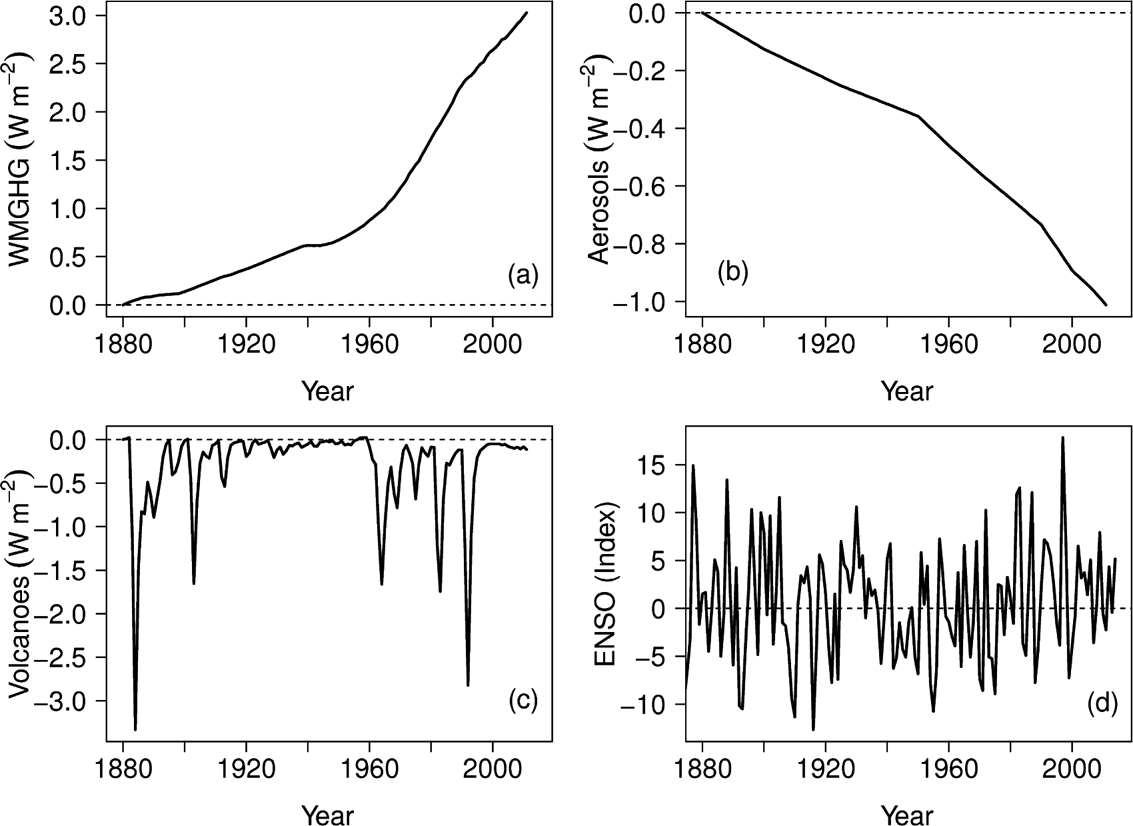
Reliable direct measurements of the major greenhouse gas, carbon dioxide, began in the International Geophysical Year (1957–58) with the ground-breaking work of Keeling (Reference Keeling1960). The original network of two monitoring stations (South Pole and Mauna Loa) has since expanded to over 225 stations today. The CO2 concentrations are available from the World Data Centre for Greenhouse Gases (http://ds.data.jma.go.jp/gmd/wdcgg). Pre-1957 estimates of carbon dioxide concentration can be derived from the gas preserved within ice-core bubbles (Etheridge et al. Reference Etheridge, Steele, Langenfelds, Francey, Barnola and Morgan1996). In a similar way, direct and ice-core-based measurements of other greenhouse gases (especially methane and nitrous oxide) have been combined to build up a history of their concentrations and forcings (Myhre et al. Reference Myhre, Myhre and Storda2001, Reference Myhre, Shindell, Bréon, Collins, Fuglestvedt, Huang, Koch, Lamarque, Lee, Mendoza, Nakajima, Robock, Stephens, Takemura, Zhang, Stocker, Qin, Plattner, Tignor, Allen, Boschung, Nauels, Xia, Bex and Midgley2013). In this present paper, the aggregated forcings have been taken from the Intergovernmental Panel on Climate Change Fifth Assessment Report (IPCC AR5) (Myhre et al. Reference Myhre, Shindell, Bréon, Collins, Fuglestvedt, Huang, Koch, Lamarque, Lee, Mendoza, Nakajima, Robock, Stephens, Takemura, Zhang, Stocker, Qin, Plattner, Tignor, Allen, Boschung, Nauels, Xia, Bex and Midgley2013, chapter 8). The IPCC greenhouse-gas concentration time-series, specifically the Coupled Model Intercomparison Project phase 5 (CMIP5) Representative Concentration Pathways (RCPs), were obtained from the multi-model data archive, http://cmip-pcmdi.llnl.gov/cmip5/data_portal.html, and converted into a radiative forcing following the conversion recommended in Joos et al. (Reference Joos, Prentice, Sitch, Meyer, Hooss, Plattner, Gerbe and Hasselmann2001, appendix A2) before plotting in Figure 1a.

Figure 1 Historical forcings: (a) well-mixed greenhouse gases; (b) aerosols; (c) volcanic aerosols; (d) El Niño-Southern Oscillation.
2.1.2. Aerosols
The second atmospheric data set needed here is the history of sulphate aerosols. Boucher & Pham (Reference Boucher and Pham2002) described how observations and regional inventories (since 1850) can be used to uncover a global mean emission history for sulphate aerosols. The crucial importance of sulphate aerosols in climate-change studies was first recognised by Charlson et al. (Reference Charlson, Schwartz, Hales, Cess, Coakley, Hansen and Hofmann1992) and elaborated upon by Mitchell et al. (Reference Mitchell, Johns, Gregory and Tett1995). Here, sulphate emissions, specifically the CMIP5 time-series as obtained from the multi-model data archive (http://cmip-pcmdi.llnl.gov/cmip5/data_portal.html) were converted into a direct radiative forcing following the straightforward scaling used by Joos et al. (Reference Joos, Prentice, Sitch, Meyer, Hooss, Plattner, Gerbe and Hasselmann2001, appendix A3). The emission estimates are plotted in Figure 1b. The reason that emission data, rather than concentration observations, can be used for aerosols is because aerosols are much shorter lived than the main anthropogenic greenhouse gases. However, it is worth bearing in mind that aerosol uncertainties are larger than those of greenhouse gases.
2.2. Natural effects
Time-series of volcanic aerosols, sunspot numbers and the El Niño-Southern Oscillation (ENSO) were also tested as regressors in the likelihood-based energy-balance model. Volcanic reconstructions of aerosol optical depth, sourced from IPCC AR5 Chapter 8 (Myhre et al. Reference Myhre, Shindell, Bréon, Collins, Fuglestvedt, Huang, Koch, Lamarque, Lee, Mendoza, Nakajima, Robock, Stephens, Takemura, Zhang, Stocker, Qin, Plattner, Tignor, Allen, Boschung, Nauels, Xia, Bex and Midgley2013), were used for the volcanic aerosol time-series (Fig. 1c). Wolff sunspot numbers (yearly, mean, total-sunspot number) were sourced from WDC-SILSO, Royal Observatory of Belgium, Brussels. The JISAO-Global-SST-ENSO index, available from http://jisao.washington.edu/data/globalsstenso, was chosen as a measure of the El Niño-Southern Oscillation (Fig 1d). The indices were used in a raw form, and not converted into forcings, as the maximum-likelihood approach used here is able to calculate its own scaling factors automatically.
2.3. Air temperature observations
Following Callendar's (Reference Callendar1949) early analyses and the detailed and painstaking work of Jones et al. (Reference Jones, Wigley and Kelly1982), many data sets of historical air-temperature changes have been developed. For example, 36 data sets (time-series) as created at the Climate Research Unit at the University of East Anglia (in conjunction with the Hadley Centre), the British Meteorological Office, NASA's Goddard Institute for Space Studies (GISS), the National Climatic Data Centre (NCDC) of the National Oceanic and Atmospheric Administration, the University of Alabama (UAH) and Remote Sensing Systems (RSS) can all be sourced at http://www.climatedata.info/Temperature/reconstructions.html. Out of the 36 data sets, the GISS, and especially the CRUTEM4 and HadCRUT4 data sets (Figs 2, 3a), were selected (on the basis of a principal-component analysis) for more detailed study. Feulner et al. (Reference Feulner, Rahmstorf, Levermann and Volkwardt2013) discuss historical differences in temperature and rates of warming over land as compared to the oceans.
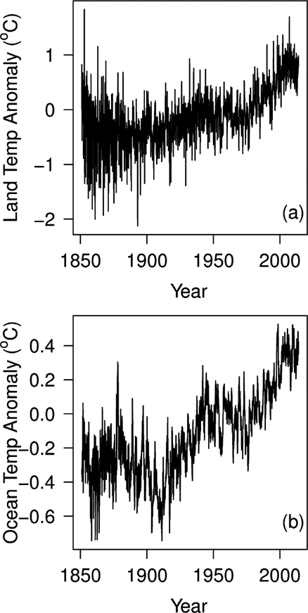
Figure 2 Global land–ocean historical temperatures: (a) temperature over land (CRUTEM4); (b) temperature over oceans (HadCRUT4). Both time-series plotted as monthly anomalies. Although the broad trends of the two time-series are similar, note how the temperature range of the land record is twice that of the ocean and how its high-frequency variation is also greater. The ocean record, in contrast, shows more medium-term fluctuations, with durations typically of 2–10 years.
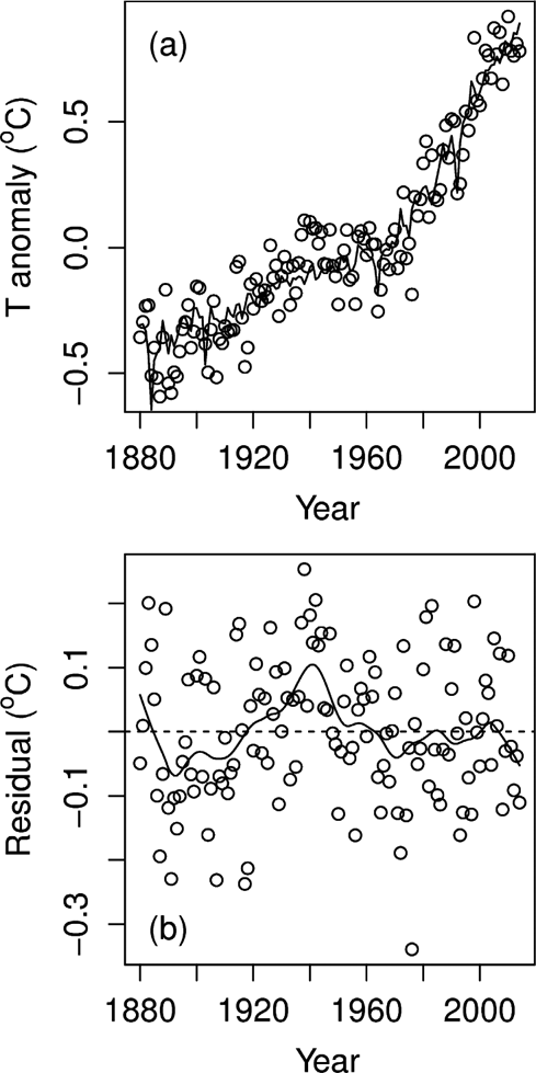
Figure 3 Fit of historical temperatures and model. In this example, GISS temperatures and a seven-parameter model are used: (a) open circles observations. Solid line energy balance model; (b) open circles residuals. Solid line LOESS (locally weighted scatterplot smoother) fit drawn to help emphasise runs of residuals of the same sign.
2.4. Modelled air temperatures
Recently, an excellent set of simulated (as opposed to observed) historical temperatures has become available as part of a new era in climate-change research, namely the Climate Model Intercomparison Project (Meehl et al. Reference Meehl, Covey, Taylor, Delworth, Stouffer, Latif, McAvaney and Mitchell2007). The most recent (fifth phase) of the Intercomparison Project (CMIP5) has generated a freely available state-of-the-art multimodel dataset of climate variability and climate change (Taylor et al. Reference Taylor, Stouffer and Meehl2012). The CMIP modelling strategy includes climate-change modelling experiments which involve long-term (century time-scale) integrations starting from a preindustrial (quasi equilibrium) state and going on to span a period from the mid-nineteenth century through the twenty-first century and beyond. Nineteen temperature data-sets were sourced from the historical CMIP5 data portal (http://cmip-pcmdi.llnl.gov/cmip5/data_portal.html) and form the basis of the validation study described below.
3. Results
The main results of this paper all basically derive from using the additive energy-balance model (of Equations 3 & 4) to generate good, parsimonious fits to the historical temperature data of Figures 2 and 3a, using solely measurement-based assessments of anthropogenic radiative forcings (Fig 1) as the regressors.
3.1. Historical temperature time-series
Figure 3a shows a typical example of an additive energy-balance model fit to an historical temperature series. In this example, GISS temperatures (global, mean, land–ocean, temperature index), are regressed against the four forcings of Figure 1. Visually, the fit looks reasonable, with no obvious discrepancies (Fig. 3a). Figure 3b plots the residuals as a time-series. An important part of all statistical model building involves a careful examination of residuals. The much discussed recent slowdown, or hiatus, in Earth's surface-temperature rise over the last 15 years is seen as a short run of negative residuals at the far right-hand edge of Figure 3b. Interestingly, this recent period does not stand out as being particularly unusual, with equally long runs of same-signed residuals occurring at other times in the past; for example, through the late 1930s and early 1940s.
3.2. Climate sensitivity
Can a useful estimate of climate sensitivity be extracted from the regression model of Figure 3? The model uses four forcings – well-mixed greenhouses gases, aerosols, volcanoes and ENSO. The constant, as determined at −0.38oC, represents an estimate of the preindustrial temperature in 1750, when the forcings were zero. As would be expected it is negative; i.e., below that of the reference period (1961–1990). The model also calculates an estimate of the exponential smoothing constant of 0.72, and an autocorrelation estimate of 0.65. Concentrating on the forcings, the most significant is found to be that of the well-mixed greenhouse gases. The value of its regression coefficient (once multiplied by a typical estimate (3.71 W m–2) for the radiative forcing for a CO2 doubling) would appear to be that of the sought-after climate sensitivity.
3.3. The aerosol dilemma
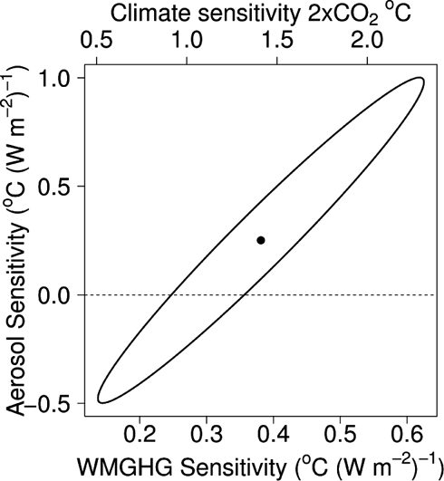
Closer inspection of the model, however, reveals a profound difficulty. Whilst many aspects are very satisfactory – the fit is reasonably good; there are few parameters to be determined; the errors associated with many of the individual regressors are small; the model behaves stably; the residuals are largely structureless – one problem nevertheless is evident (Fig. 4). The correlation between the regression parameters for the well-mixed greenhouse gases and the aerosols is worryingly large (0.97). This simple statistical result (strong correlation between regressors) flags up a potentially profound underlying problem. That is, when two variables are very strongly correlated, the regression is able to infer very precisely the sum of their two effects; but is unable to infer their individual effects. The 95 % confidence ellipse in Figure 4 illustrates this dichotomy whereby high climate sensitivity is associated with large (positive) aerosol scaling factors, whilst low GHG sensitivities (a factor of five lower) arise in conjunction with negative aerosol scaling factors. Wigley & Santer (Reference Wigley and Santer2013) have similarly drawn attention to this situation, whereby aerosol cooling offsets GHG-induced warming. In order to make progress with the regression modelling, the between-parameter correlation needs to be pared down.

Figure 4 95 % confidence ellipse. The elongated ellipse results from the high correlations between regression parameters of the underlying model. NB: the CMIP5 aerosol forcing is negative through the historical period; hence, positive aerosol scaling factors correspond to cooling.
A visual examination of the predictors of Figure 1 suggests that the most likely cause of the unwanted between-parameter correlation is the statistical problem of collinearity. In brief, the ‘shapes’ of the well-mixed greenhouse gases and aerosols time-series (of Figs 1a and 1b) are close to being mirror images of each other. Both time-series change slowly at first and then, after the mid-1900s, more rapidly. Thus the model includes factors which are correlated not just with the response variable, but also with each other.
When using linear regression for building a purely empirical model, the solution to such multicollinearity problems can be relatively simple. For example, the removal of one of the highly correlated predictors from the model by using stepwise regression, or cutting down on the number of predictors using principal components regression, are widely adopted tactics. Here, however, as there are physical reasons for believing that the relationship between the response and the predictors follows a particular functional form, another approach is desirable. Consequently, instead of the above tactic of modifying the right-hand side of the regression equation, by improving the x-values, betterment is sought by enhancing the y-values on the left-hand side.
3.4. An expanded model
An upgraded model is next tried, in which land and ocean temperatures, rather than just global temperatures, are used as the model response (i.e., as the y-values). The lifetimes of most aerosols are short and therefore their geographical distribution is strongly related to their sources. As a consequence, aerosol optical depth is greater over the northern hemisphere than over the southern hemisphere, and greater over the land than over the oceans. It is this geographical difference which lies at the heart of how an improved model can be constructed to confront the collinearity dilemma. In addition, in the upgraded model, a second thermal time-constant is added, in order to allow the land and ocean temperatures to evolve individually. In short, the idea is to model the difference between the land and ocean temperatures, over the late-nineteenth and twentieth centuries (contrast Figs 1a and 1b), by allowing distinct thermal time-constants and aerosol optical depths.
The expanded model, along with its confidence intervals, is most straightforwardly derived from bootstrap prediction. Care was taken to use a moving (circular) block bootstrap (Efron & Tibshirani Reference Efron and Tibshirani1994) in order to preserve the temporal autocorrelation structure. Figure 5 plots the bootstrap estimates for the temperature sensitivity to a doubling of CO2 against the aerosol scaling factor, along with their histograms. The bootstrap still finds a strong correlation between the two predictors, as shown in Figure 5 by the diagonal (lower left to upper right) spread of estimates. But now, the aerosol scaling factor (which includes both direct and indirect effects) is significantly different from zero. A best (‘data driven’) estimate of the climate sensitivity is +4oC, with 95 % confidence intervals of 3.0oC to 6.3oC. The top histogram shows the spread of climate sensitivities, with a long low tail stretching out to high values. The time-constants found by the model (in terms of half-lives) are 48 years (oceans) and 1.2 years (land). The model assessment of the relative importance of the aerosol effect over land as compared to over the ocean is 79 % (land) and 21 % (ocean).
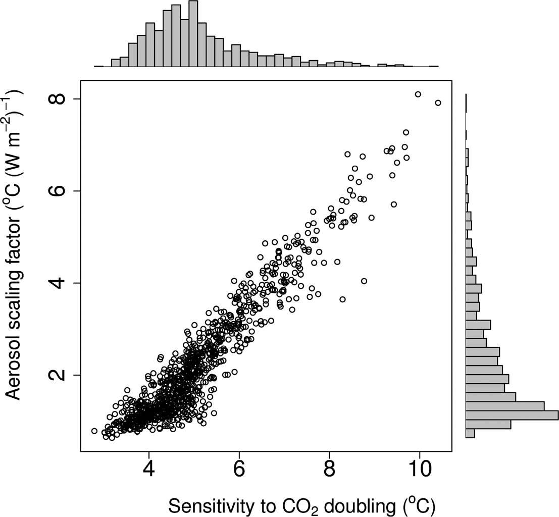
Figure 5 Using the bootstrap as an analytical tool. Scatterplot and histograms of the temperature change due to a doubling of CO2 and of the aerosol scaling factor.
Figure 6, in addition to the model fit, plots future temperature projections. Land temperatures are predicted, by 2100, to rise by almost 8oC above preindustrial; ocean temperatures by roughly half that. The projections are obtained as follows. First the land- and ocean-temperature observations are fitted simultaneously using the expanded energy-balance model. Then, the resulting regression parameters are used to estimate future temperature change based on the radiative forcings of the Representative Concentration Pathway scenario RCP8.5. RCP8.5 is a ‘business-as-usual’ climate change scenario (currently emissions are tracking slightly above RCP8.5; see Peters et al. Reference Peters, Andrew, Boden, Canadell, Ciais, Le Quéré, Marland, Raupach and Wilson2013). Confidence bands are also included in Figure 6. The bands are estimated using the bootstrap procedure, which can be seen to generate asymmetrical confidence intervals.
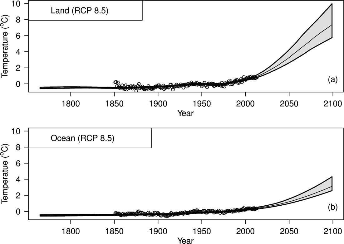
Figure 6 Model fit to historical land (a) and ocean (b) temperature records (open circles), and temperature forecast to the year 2100 as based on RCP8.5. Note how both time-series work out to have similar (i.e., not significantly different) pre-industrial temperatures; and how land temperatures are predicted to rise by almost 8oC above preindustrial levels, and ocean temperatures by 4oC, by the year 2100. Confidence region plotted in grey.
3.5. Validation
Full verification and validation of numerical models of natural systems is impossible: we only have one Earth. Nevertheless, their underlying mathematics, coding, bias and applicability can, to a certain extent, be checked (see for example Foster et al.'s (Reference Foster, Annan, Schmidt and Mann2008) and Knutti et al.'s (Reference Knutti, Kraehenmann, Frame and Allen2008) appraisals of Schwartz's (Reference Schwartz2007) proposed climate model). For simple climate models, a useful approach is to test the modelling methodology proposed for the real Earth on computer-based simulations of the twentieth-century climate, as generated by ‘state-of-the-art’ three-dimensional, coupled atmosphere–ocean, general circulation models (AOGCMs). Figure 7 illustrates the outcome of this approach to validation. In it, climate sensitivities from nineteen ‘state-of-the-art’ models are compared to those obtained by the simple energy-balance model as developed in this paper.
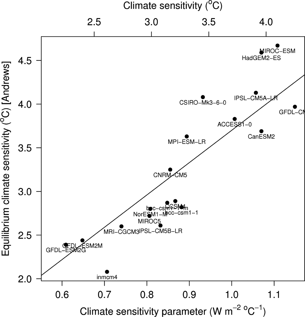
Figure 7 CMIP5 multi-model ensemble. Comparison of the additive model (Equations 3 & 4) approach with Gregory et al.'s. (Reference Gregory, Ingram, Palmer, Jones, Stott, Thorpe, Lowe, Johns and Williams2004) method (using an abrupt 4×CO2 change) for diagnosing climate sensitivity (see Andrews et al. Reference Andrews, Gregory, Webb and Taylor2012). The lettering is the ‘official’ model name for each modelling group.
The nineteen models are all taken from phase 5 of the recent World Climate Research Programme's (WCRP's) Coupled Model Intercomparison Project (CMIP5). Each model is from a different modelling group. For each model, the equilibrium climate sensitivity was obtained from the CMIP5 abrupt CO2 quadrupling experiments (Taylor et al. Reference Taylor, Stouffer and Meehl2012). (See Gregory et al. (Reference Gregory, Ingram, Palmer, Jones, Stott, Thorpe, Lowe, Johns and Williams2004), Andrews et al. (Reference Andrews, Gregory, Webb and Taylor2012) and Forster et al. (Reference Forster, Andrews, Good, Gregory, Jackson and Zelinka2013) for further details.)
Next, land and ocean temperatures from the AOGC model output, from each modelling group, were obtained for the historical period and then analysed using the improved energy-balance model of section 3.4. Figure 7 plots the CMIP5 quadrupling experiment sensitivities against the sensitivities estimated by the energy-balance approach. Agreement between the two approaches is seen to be generally very reasonable. In particular, the sensitivities are seen to cluster well about the diagonal line, which denotes the trend for complete agreement.
4. Discussion
Climate models of varying complexity exist. They range from simple empirical models, through more sophisticated intermediate-complexity models, to comprehensive, physically based, coupled, general circulation models of the atmosphere and the ocean, which incorporate processes including biogeochemical cycles. All models have their own individual strengths and weaknesses. The principal advantage of the regression approach used here is its simplicity and interpretability, and the transparency of the model formulation. Nevertheless, it is important to be cautious about results obtained from a regression analysis and to remain alert to potential flaws, problems and pitfalls.
Regression is a vast topic. In linear regression, commonly encountered difficulties include: the data used in fitting the model are not fully representative; the drawback that in reality most systems are not linear; the inclusion of too many independent variables which can cause serious difficulties; dependence among variables which can lead to unsound predictions; poor selection of the independent variables which may uncover spurious relationships that only happen to be there by chance; overlooking hidden variables; forgetting uncertainty (noise) in the independent variables, thereby obscuring the exact relationship between the dependent and independent variables; the residuals are not independent; and the problem of outliers. Fortunately, once one is aware of potential difficulties, there are many well-known checks and techniques available to help guard against the problems.
Here, in order to avoid gross model misspecification, the functional relationships between the variables were carefully considered. In particular, the modelling started simply, and was only made more complex when needed. Moreover, prior studies (GCMs) were used to help determine which variables to try in the regression model. In addition, wherever possible, large numbers of trustworthy data and a small number of predictors were selected. Stepwise-type calculations demonstrated that the inclusion of non-linear amalgamations of model parameters was not necessary. Finally, residual analysis was used to guard against unusual observations, autocorrelation, unequal variances (heteroscedasticity) and model misspecification.
The Sun has an obvious effect on climate, since it is the main energy source for the radiative budget of the Earth. Nevertheless, solar variation was not found, in any of the models examined here, to be an effective regressor for temperature change. It is worth commenting at the outset that in this paper, solar variation was restricted to the sunspot cycle. A solar variation in irradiance which includes an additional hypothetical long-term trend, as often used in climate-change studies (e.g., reconstruction of total irradiance by Lean et al. (Reference Lean, Beer and Bradley1995)), will inevitably, in a simple regression analysis, be difficult to disentangle from other regressors with a largely monotonic trend. Here, the strong preference is for regressors with solid, observational evidence (e.g. Wolff sunspot numbers), rather than those based on calculation, or on fragmentary datasets.
Volcanic and El Niño effects were found to be of consequence. These were discerned to be significant, albeit modest, regressors. Their inclusion in the models improved the fit, increased the adjusted R-squared, and slightly improved the confidence limits of the regressor coefficients. Any future changes in these two natural forcings are obviously unknowable, so their average value, through the historical time period, was used in the future scenario calculations.
Next, in order of importance, come the atmospheric (sulphate) aerosols. These turned out to be crucial in the regression models. The aerosol regression coefficient, of course, incorporates everything that is linearly related to the aerosol forcing (all indirect aerosol effects including those associated with cloud condensation effects, cloud amount, liquid-water content and ice effects) as well as the direct effect of the aerosols themselves. The total (direct plus indirect) effect was found to be significant (Fig. 6). Its sign shows that the net effect of aerosols, throughout the historical period, has been to generate a noticeable cooling.
Finally, the most important regressor is that of well-mixed greenhouse gases with a climate sensitivity of +4oC, for a CO2 (equivalent) doubling. This is the change CO2 is predicted to make in temperature, when all the other regressors are held constant (Fig. 6). As has often been pointed out, CO2 is a key determinant of future climate, not only because it is a strong greenhouse gas (as seen in the regression model), but also because it is a long-lived gas. Thus, millennial-lived gases, such as CO2, are likely to be by far the most important mediators of anthropogenic climate disruption (Eby et al. Reference Eby, Zickfeld, Montenegro, Archer, Meissner and Weaver2009; Pierrehumbert Reference Pierrehumbert2014). Eby et al.'s (Reference Eby, Zickfeld, Montenegro, Archer, Meissner and Weaver2009) modelling of the release of carbon dioxide by combustion, its equilibration in the atmosphere, ocean and terrestrial biosphere and very slow return to solid Earth suggests that the lifetime of the ensuing surface air-temperature anomaly will be longer than the lifetime of anthropogenic CO2. That is, slow oceanic and weathering processes cause the anthropogenic temperature anomaly to persist for many millennia. As Eby et al. (Reference Eby, Zickfeld, Montenegro, Archer, Meissner and Weaver2009) point out, “it is sobering to ponder the notion that the carbon we emit over a handful of human lifetimes may significantly affect the earth's climate over tens of thousands of years”.
The recent slowdown in Earth's surface-temperature rise has been rationalised by a wide range of scientific explanations. Recently, Roberts et al (Reference Roberts, Palmer, McNeall and Collins2015), using an observationally constrained ensemble of GCMs and a statistical approach, have provided further robust evidence that the slowdown is an integral component of current climate models and so deserves explanation. Most discussions revolve around explaining why temperatures have been low. Here, however, the anomaly is seen to relate equally to higher-than-expected temperatures during the early part of the slowdown (a run of positive residuals) as to lower-than-expected temperatures during the later stages. An alternative underlying cause for the slowdown could then involve heat initially moving from deep waters to the surface, rather than vice-versa.
The new energy-balance equation can easily be extended to test other potential forcings. For example, black carbon (Bond et al. Reference Bond, Doherty, Fahey, Forster, Berntsen, DeAngelo, Flanner, Ghan, Kärcher, Koch, Kinne, Kondo, Quinn, Sarofim, Schultz, Schulz, Venkataraman, Zhang, Zhang, Bellouin, Guttikunda, Hopke, Jacobson, Kaiser, Klimont, Lohmann, Schwarz, Shindell, Storelvmo, Warren and Zender2013) was added, but found to have sensitivities ranging from −1.5 W m–2 to +0.5 W m–2 (very similar to Bond et al.'s (Reference Bond, Doherty, Fahey, Forster, Berntsen, DeAngelo, Flanner, Ghan, Kärcher, Koch, Kinne, Kondo, Quinn, Sarofim, Schultz, Schulz, Venkataraman, Zhang, Zhang, Bellouin, Guttikunda, Hopke, Jacobson, Kaiser, Klimont, Lohmann, Schwarz, Shindell, Storelvmo, Warren and Zender2013) large range), and so was not investigated further. In the same way, a heat transport term, based on the land–ocean temperature difference, was tested but found to be unnecessary. The energy-balance equation can also be used to generate hind casts (also called historical re-forecasts) starting from any date. For example, hind cast ensembles through the period of the recent temperature slowdown were obtained for start dates ranging from 1997 through to 2013. The hind casts were found to be robust to start date. The early years of the temperature slowdown were always re-forecast at very similar levels (i.e., around 0.1oC lower than observed).
5. Conclusions
Well-mixed greenhouse gases (WMGHG), aerosols, volcanoes and ENSO are all found to be significant forcings of global temperature during the historical time period.
• No significant hiatus in temperature rise, over the last decade and a half, is revealed by formal residual analysis or run tests. The recent temperature slowdown is not unusual. Similar slowdowns are found in simulated historical temperatures produced in the Climate Model Intercomparison Project, and in observed temperatures in the late-nineteenth and mid-twentieth centuries.
• The recent slowdown in temperature rise can be explained by warmer-than-expected years in the early 2000s.
• A heat-balance model has been coded as a simple function in R. When applying the heat-balance model to historical temperatures, F-tests demonstrate the need for thermal time-constants and for AR1-type errors.
• F-tests demonstrate no need for inclusion of the sunspot cycle, nor for non-linear combinations of the model parameters.
• Whilst the sum of the anthropogenic-forcings sensitivity (aerosols+WMGHG) is well determined, the individual sensitivities remain highly correlated, and so cannot easily be disentangled.
• The basic heat-balance method has been validated on ‘state-of-the-art’ GCMs, with independently determined sensitivities.
• A ‘data-driven’ estimate of equilibrium climate sensitivity is +4oC, with 95 % confidence intervals of 3oC to 6.3oC.
6. Acknowledgements
David Stevenson and Tim Osborn are thanked for helpful discussions.
7. Appendix. R-code for a 2-regressor version of the heat balance model of Equations 3 and 4
A nonlinear model fit is accomplished by gnls() using generalised least squares. HoltWinters() performs an exponential smoothing. The smoothing constant (alpha) is constrained to lie within the range 0 to 1 by the inverse logit transform, plogis(). The model is non-linear, but nevertheless robust (relatively insensitive) to the choice of starting values; as the non-linearity is, in essence, only needed to accommodate the temporal autocorrelation within the data. Here, the parameters of the four models (b0, b1, b2, b3) are simply initialised at 1.