


1. Background
The transitioning of boundary layers (BLs) from a laminar to a turbulent regime is considered a potential ‘mission killer’ in atmospheric-entry and hypersonic-cruise flights. After transitioning, the surface heat flux can increase by up to an order of magnitude (Wright & Zoby Reference Wright and Zoby1977; Reed et al. Reference Reed, Kimmel, Schneider and Arnal1997). The inaccurate prediction capabilities regarding the streamwise location where such regime change occurs restricts engineers to overly conservative designs. The necessarily high safety coefficients on the thermal protection system (TPS) thickness, in return, penalise the available payload and the mission cost. The path forward, towards more optimised vehicle and mission design, must be founded on physics-based models that provide not only predicting capabilities, but also a level of modelling modularity that allows for a meticulous decoupling of the multiple coexisting phenomena.
Hypersonic-cruise and atmospheric-entry missions often feature an ablative TPS made of a composite material, where the surface heat fluxes are alleviated by the resin's pyrolysis and the fibres’ ablation (Laub, Wright & Venkatapathy Reference Laub, Wright and Venkatapathy2008; Milos & Chen Reference Milos and Chen2013). This process affects the development of instabilities, and ultimately conditions the transition dynamics of the BL through three main mechanisms: the modification of the surface roughness owing to the irregular decomposition of the TPS, the injection of pyrolysis gases into the BL and the modification of the gas chemistry owing to its interaction with the TPS.
High levels of surface roughness have been observed experimentally to bypass natural transition mechanisms, and therefore lead to an earlier transition (Schneider Reference Schneider2008a,Reference Schneiderb). Computational investigations also looked into how roughness-induced perturbations enter the BL (for instance Tumin Reference Tumin2008; Balakumar Reference Balakumar2013), and how they develop both for isolated (Choudhari et al. Reference Choudhari, Li, Chang, Edwards, Kegerise and King2010, Reference Choudhari, Li, Bynum, Kegerise and King2015) and distributed roughness elements (Hein et al. Reference Hein, Theiss, Di Giovanni, Stemmer, Schilden, Schröder, Paredes, Choudhari, Li and Reshotko2019; Iyer, Muppidi & Mahesh Reference Iyer, Muppidi and Mahesh2011; Shrestha & Candler Reference Shrestha and Candler2019), explaining the experimental observations. Strategically designed distributed roughness has also been reported to damp instabilities under certain conditions (Fransson et al. Reference Fransson, Talamelli, Brandt and Cossu2006; Fong et al. Reference Fong, Wang, Huang, Zhong, McKiernan, Fisher and Schneider2015). The aforementioned studies were focused on roughness elements with regular shapes, whereas the influence of the irregular roughness introduced by ablation on transition remains largely unknown. The major hurdle encountered in such studies are the logistic challenges of acquiring reliable and meaningful experimental data (Martin et al. Reference Martin, Grossir, Miró Miró, Le Quang and Chazot2019).
In contrast to the case-dependent observations reported on the effect of roughness on stability, surface mass injection has been observed consistently to destabilise the BL and consequently to advance transition upstream. Wall suction was seen to have the opposite effect. Qualitatively equivalent results were obtained in both experimental (see Berry, Nowak & Horvath (Reference Berry, Nowak and Horvath2004) and the review by Schneider (Reference Schneider2010)) and computational investigations by Malik (Reference Malik1989a), Johnson, Gronvall & Candler (Reference Johnson, Gronvall and Candler2009), Li et al. (Reference Li, Choudhari, Chang and White2013) or Shrestha (Reference Shrestha2019). Miró Miró & Pinna (Reference Miró Miró and Pinna2018), however, did report a strong variance of the predictions depending on the characteristics of the porous surface through which the injection is performed. A continuously blowing wall, mimicking the behaviour of an ablating TPS, lead to the highest perturbation growth rates and the soonest predictions of the transition-onset location.
Regarding the effect of air chemistry and gas–surface interaction on BL instability development, a major constraint is the lack of experimental results for the validation of the various models. Existing high-enthalpy hypersonic ground test facilities are unable to sustain sufficiently long test times in order to reach the chemical activity encountered in real flights (Hornung Reference Hornung1992; Itoh et al. Reference Itoh, Ueda, Komuro, Sato, Tanno and Takahashi1999; Hannemann, Schramm & Karl Reference Hannemann, Schramm and Karl2008). Flight tests thus remain the only source of experimental data; examples can be found in Johnson et al. (Reference Johnson, Stainback, Wicker and Boney1972), Walker et al. (Reference Walker, Sherk, Shell, Schena, Bergmann and Gladbach2008), Kimmel et al. (Reference Kimmel, Adamczak, Paull, Paull, Shannon, Pietsch, Frost and Alesi2015) or Wheaton et al. (Reference Wheaton, Berridge, Wolf, Stevens and McGrath2018). However, these experiments feature a major uncertainty in the free-stream conditions, offer very limited data owing to engineering challenges and are scarce because of their cost. Moreover, experiments or flight tests can very rarely provide the effective and reliable decoupling of the coexisting physical phenomena that is needed for the ultimate understanding of the transition dynamics.
Numerical investigations therefore constitute the most active field of research in high-enthalpy chemically reactingtransition investigations. The vast majority of them rely on linear perturbation theories, such as linear stability theory (LST; Mack Reference Mack1984) or linear parabolised stability equations (LPSEs; Bertolotti, Herbert & Spalart Reference Bertolotti, Herbert and Spalart1992), allowing conclusions to be drawn on the effect of the high-enthalpy phenomena on the propagation of the perturbations in the BL and its transition to turbulence. Malik (Reference Malik1989a) and Malik & Anderson (Reference Malik and Anderson1991) were the first to consider high-temperature effects, by investigating a self-similar BL with local thermodynamic equilibrium (LTE) and in calorically perfect gas (CPG) hypotheses. They observed that the internal-energy excitation and molecular dissociation in equilibrium, accounted for by the LTE but not by the CPG assumption, increased the perturbation growth rates and decreased the frequency. Stuckert & Reed (Reference Stuckert and Reed1994) extended the analysis to chemical non-equilibrium (CNE) conditions including the effect of finite-rate chemistry, and concluded that endothermic reactions increase the region of relative supersonic flow and reduced the second-mode frequency. This trend was exacerbated in equilibrium conditions. Later, Hudson, Chokani & Candler (Reference Hudson, Chokani and Candler1997) extended the theoretical framework to account also for thermal non-equilibrium (TNE), employing two separate temperatures for the vibrational and the translational–rotational energy modes. They observed a mild stabilisation owing to TNE, because the thermochemical non-equilibrium (TCNE) predictions lied between the CNE (in vibrational equilibrium) and the CPG predictions (vibrationally frozen). However, this assertion was challenged by Bertolotti (Reference Bertolotti1998), who observed that vibrational relaxation was only destabilising in flat plates, but not in blunt geometries. Miró Miró et al. (Reference Miró Miró, Beyak, Mullen, Pinna and Reed2018) looked at the effect of ionisation, by comparing a 5-species and 11-species assumption, observing it to be destabilising in CNE and LTE conditions. Klentzman & Tumin (Reference Klentzman and Tumin2013) investigated binary oxygen mixtures, isolating the stabilising contribution of viscosity to second-mode growth by comparing inviscid and viscous perturbation hypotheses. They also compared various levels of surface catalysis, concluding that the increased wall temperature, associated with the catalytic exothermic reactions, stabilised the second mode. Mortensen & Zhong (Reference Mortensen and Zhong2016) extended the theoretical gas-chemistry framework by including an ablative boundary condition in their investigations, and studied the transition dynamics of blunt cones. Their framework also accounted for the energy radiated from the graphite surface. However, they focused exclusively on the effect of the multiple coexisting phenomena combined, and withheld from performing an exhaustive analysis of their isolated effect on second-mode instabilities.
Unstable supersonic second-mode waves (often referred to as ‘supersonic modes’) have been repeatedly observed in high-enthalpy scenarios. Such modes radiate energy into the freestream, with a significantly slower decay of the perturbation amplitude function in the wall-normal direction that must be taken into consideration when discretising the computational domain. They were first reported by Mack (Reference Mack1984) in CPG conditions, but their study recently gained momentum after the exhaustive parametric investigation by Bitter & Shepherd (Reference Bitter and Shepherd2015) in TNE, and later by Knisely & Zhong (Reference Knisely and Zhong2019a,Reference Knisely and Zhongb,Reference Knisely and Zhongc) in TCNE. They observed supersonic modes to appear as a consequence of highly cooled walls. Mortensen (Reference Mortensen2018) also reported unstable high-frequency supersonic modes in vehicles with strong nose bluntness. The studies featured a stronger destabilisation of such modes in situations with molecular dissociation, in agreement with the early observations by Chang, Vinh & Malik (Reference Chang, Vinh and Malik1997), who noted their appearance only in LTE or CNE, and not in CPG conditions. The recent results by Miró Miró et al. (Reference Miró Miró, Beyak, Mullen, Pinna and Reed2018) in hot-wall BLs, yet with chemistry-driven cooling, suggest that it is indeed the reduction of the BL temperature that promotes unstable supersonic modes, regardless of whether the cooling is a consequence of the wall temperature or of the chemical activity in the bulk of the gas. The slow decay of supersonic modes implies that there may exist a non-negligible interaction with the shock wave, which could be investigated with appropriate freestream perturbation boundary conditions, such as the linearised Rankine–Hugoniot relations employed by Esfahanian (Reference Esfahanian1991), Stuckert & Reed (Reference Stuckert and Reed1994) or Pinna & Rambaud (Reference Pinna and Rambaud2013), among others.
Researchers, such as Marxen et al. (Reference Marxen, Magin, Shaqfeh and Iaccarino2013), Ma & Zhong (Reference Ma and Zhong2004), or Mortensen & Zhong (Reference Mortensen and Zhong2016), opted for a more physically general modelling framework than the mentioned stability theories, and performed direct numerical simulations (DNS) of the full Navier–Stokes (NS) equations. This approach is also substantially more computationally demanding, making it operationally impossible to perform extensive parametric studies.
The aforementioned investigations featured a wide variety of thermophysical models, because the mathematical description of high-temperature gas properties has remained a very active field of research over the past century; see the work of Chapman & Cowling (Reference Chapman and Cowling1939), Hirschfelder, Curtiss & Bird (Reference Hirschfelder, Curtiss and Bird1954), Blottner, Johnson & Ellis (Reference Blottner, Johnson and Ellis1971), Gupta et al. (Reference Gupta, Yos, Thompson and Lee1990), Fertig, Dohr & Frühauf (Reference Fertig, Dohr and Frühauf2001), McBride, Zehe & Gordon (Reference McBride, Zehe and Gordon2002), Magin & Degrez (Reference Magin and Degrez2004), Scoggins (Reference Scoggins2017) or Clarey & Greendyke (Reference Clarey and Greendyke2019). This motivated the investigations on the sensitivity of LST predictions to the thermophysical modelling by Lyttle & Reed (Reference Lyttle and Reed2005), Franko, MacCormack & Lele (Reference Franko, MacCormack and Lele2010) and, most thoroughly, by Miró Miró et al. (Reference Miró Miró, Beyak, Pinna and Reed2019a). The latter reported that second-mode instabilities were mostly affected by modelling inaccuracies that translated into a misestimation of the BL height. Specifically, the use of a transport model (appendix A.2) with a 10 % inaccuracy with respect to the state of the art (appendix A.1), lead to an error in the predicted transition-onset location of 38 %. The early investigations by Elliott et al. (Reference Elliott, Greendyke, Jewell and Komives2019) also suggested a non-negligible variability of the predictions associated with the gas–surface interaction modelling.
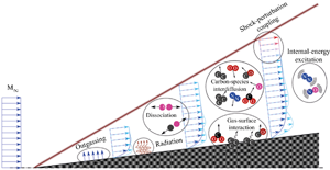
Within the aforementioned framework, this work presents and employs an effective methodology for the decoupling of many of the coexisting physical phenomena in an ablation-transition problem, together with a quantification of their relative contribution to second-mode perturbation development. The development of instabilities is described employing LST together with the semi-empirical  $\textrm {e}^\textrm {N}$ method (see van Ingen Reference van Ingen1956 and Smith & Gamberoni Reference Smith and Gamberoni1956). A variety of boundary conditions and thermophysical flow assumptions are employed in order to isolate the contributions (sketched in figure 1) of: internal-energy-mode excitation, ablation-driven outgassing, ablation- and radiation-induced wall cooling, the interdiffusion of dissimilar species, dissociation reactions occurring between air and carbon species, surface chemistry and radiation and perturbation–shock interactions. The significance of these phenomena is evaluated on a graphite wedge at four flight-envelope points in an aggressive atmospheric entry mission. For the sake of simplicity and in the pursuit of feasible computational times, tests feature a smooth surface and a unique temperature to describe the thermodynamic state of the gas, thus effectively neglecting ablation-induced surface roughness and TNE effects. Similarly, analyses are restricted to second-mode waves, known to be dominant in flows over sharp wedges or cones at
  $0^\circ$ pitch and yaw, in the absence of surface excrescences. Two different sets of high-temperature transport models are also compared, in order to evaluate the modelling assumptions made by Mortensen & Zhong (Reference Mortensen and Zhong2016) in their ablation-transition investigation, against the state of the art. This comparison also assesses whether the strong dependency of the predictions on the transport model, observed by Miró Miró et al. (Reference Miró Miró, Beyak, Pinna and Reed2019a), extends to more complex physical scenarios.

Figure 1. Sketch of the various physical phenomena under consideration.
2. Flow modelling
Various flow assumptions are employed, featuring marginally increasing levels of modelling complexity and generality, in order to isolate the different phenomena associated with such marginal improvement. For example, if one has four physical phenomena ( $A$,
$A$,  $B$,
$B$,  $C$,
$C$,  $D$) and is interested in identifying the individual contribution of phenomenon
  $B$, this can be achieved by comparing the predictions made with a flow assumption accounting for
  $A$ and
  $B$ (say flowAB), to those made with a flow assumption accounting solely for
  $A$ (say flowA). The modification of the perturbation behaviour (
 $q'_B$) owing to
  $B$ is thus equal to
  $q'_{{flowAB}} - q'_{{flowA}}$.
Extending the previous example to the actual flow under consideration, the influence on instability growth of the phenomenon of internal-energy excitation can be isolated by comparing the predictions done with a CPG and a thermally perfect gas (TPG) flow assumption. CPG assumes a linear thermal law, neglecting vibrational and electronic excitation, whereas TPG assumes a nonlinear law that does not neglect them. The modification of the perturbation behaviour owing to internal-energy excitation is thus equal to  $q'_{TPG} - q'_{CPG}$.
The previous example, showing how the contributions of internal-energy-mode excitation is isolated, is presented solely to outline the motivation for the use of the multiple flow assumptions and boundary conditions introduced subsequently in this section and the following (§ 3). The full phenomenon-decoupling methodology is laid out in § 4 for all the phenomena sketched in figure 1.
Depending on the flow assumptions, the system's equations vary slightly. An overview of these differences is given in the present section.
2.1. Tensorial notation and the invariant form
The equations in this work are presented in their invariant form, making them valid with independence of the coordinate system, and featuring the metric tensor  $g_{ij}$. This allows us to keep track of not only the variable value changes, but also of the modification of the space itself owing to such basis changes. It is defined as
 \begin{equation} g_{ij} = \sum_{k=1}^{3} \frac{\partial \mathscr{X}^k}{\partial x^i} \frac{\partial \mathscr{X}^k}{\partial x^j}, \end{equation}
where  $\mathscr {X}^i$ corresponds to the Cartesian coordinates, and
  $x^i$ to the actual coordinate system to be employed. For a Cartesian coordinate system,
  $g_{ij}$ is simply equal to the Dirac delta function
  $\delta _{ij}$. The contravariant metric tensor (
 $g^{ij}$) is simply the inverse of the covariant (
 $g_{ij}$). Moreover, the expressions presented feature velocities (
 $u^i$) in the non-Cartesian reference frame (
 $x^i$ rather than
  $\mathscr {X}^i$). Velocities in the Cartesian reference frame (
 $\mathscr {U}^i$) can be obtained through
 \begin{equation} \mathscr{U}^i = \sqrt{g_{ii}}\,u^i , \quad \forall i\in[1,2,3] . \end{equation}
The superscript/subscript notation refers to contravariant/covariant vectorial variables. A vectorial variable is contravariant  $q^i$ when its components vary with the inverse transformation with respect to the basis change, that is, they ‘contra-vary’. On the other hand, it is covariant
  $q_i$ if its components vary with the same transformation, that is, they ‘co-vary’. A spatial covariant derivative is expressed with a comma followed by an index corresponding to the spatial direction with respect to which one is deriving:
  $q^i_{,j}$. The comma derivative notation is restricted to spatial derivatives. For the sake of notational simplicity, the spatial subindices are strictly kept as
  $i$,
$i$,  $j$,
$j$,  $k$ and
  $l$ throughout the text. Therefore, variable subindices containing commas followed by other symbols are not to be regarded as derivatives. The evaluation of covariant derivatives must be done also taking into consideration the curving of the space itself:
 \begin{equation} q^j_{,k} = \frac{\partial q^j}{\partial x^k} + \varGamma^j_{ik} q^i , \end{equation}
which features the Christoffel symbol of the second kind
 \begin{equation} \varGamma^j_{ik} = \sum_{l=1}^{3} \frac{1}{2 g^{jl}} \left(\frac{\partial g_{li}}{\partial x^k} + \frac{\partial g_{lk}}{\partial x^i} - \frac{\partial g_{ik}}{\partial x^l}\right) . \end{equation}
A short introduction to tensorial algebra can be found in Pinna & Groot (Reference Pinna and Groot2014) and Miró Miró (Reference Miró Miró2020). For more details, one should refer to the work of Brillouin (Reference Brillouin1964) and Aris (Reference Aris1962).
2.2. Flow equations
A dilute mixture of gases in CNE can be modelled with a separate mass-conservation equation for each species (2.5a), three momentum equations (2.5b) and an energy equation (2.5c):
 \begin{gather} \frac{\partial \rho_s}{\partial t} + (u^j \rho_s)_{,j} = - J_{s,j}^j + \dot{\omega}_s, \quad \forall s \in \mathcal{S}, \end{gather}
 \begin{gather}\rho \frac{\partial u^i}{\partial t} + \rho u^j u^i_{,j} = -g^{ij} p_{,j} + \mathbb{T}^{ij}_{,j}, \quad \forall i \in [1,2,3] , \end{gather}
 \begin{gather}\rho \frac{\partial h}{\partial t} + \rho u^j h_{,j} = \frac{\partial p}{\partial t} + u^j p_{,j} + (\kappa^{Fr} \,g^{ij} T_{,i})_{,j} - \mathcal{J}^j_{,j} + g_{ik} \mathbb{T}^{kj} u^i_{,j} , \end{gather}
where  $t$ is time,
  $\rho _s$ is the partial density of each species
  $s$,
$s$,  $\rho$ is the density of the mixture,
  $\mathcal {S}$ is the set of all species,
  $p$ is the mixture pressure,
  $\mathbb {T}^{ij}$ is the viscous stress tensor,
  $h$ is the mixture enthalpy,
  $\kappa ^{Fr}$ is the frozen thermal conductivity,
  $J_s$ is the species mass diffusion flux,
  $\omega _s$ is the species mass production rate and
  $\mathcal {J}^j$ is the total-energy diffusion flux. The full nomenclature used in this article is listed in the supplementary material available at https://doi.org/10.1017/jfm.2020.804.
Alternatively one may substitute the mass-conservation equation of one of the species with the mixture continuity equation:
 \begin{equation} \frac{\partial \rho}{\partial t} + (u^j \rho)_{,j} = 0 . \end{equation}
In order to have a well-conditioned system of equations, it is preferable to enforce (2.6) instead of the mass conservation (2.5a) of the bath species (largest mass fraction), as proposed by Stuckert (Reference Stuckert1991).
The viscous stress tensor is defined as
 \begin{equation} \mathbb{T}^{ij} = \lambda g^{ij} u^k_{,k} + \mu \left(g^{jk} u^i_{,k} + g^{ik} u^j_{,k}\right) , \end{equation}
where  $\mu$ and
  $\lambda$ are the first and second dynamic viscosity coefficients. A Maxwellian reactive regime is assumed, justifying the absence of a reactive pressure term in (2.5b) (see Giovangigli Reference Giovangigli1999). Body forces are also neglected, owing to the high speeds under investigation.
The energy diffusion flux is defined as
 \begin{equation} \mathcal{J}^j = \sum_{s\in\mathcal{S}} h_s J^j_s , \end{equation}
where  $h_s$ is the species enthalpy.
A TPG, in general, requires the same equation set as a gas in CNE, yet neglects the species source term ( $\dot {\omega }\approx 0$). However, when there is no surface injection of dissimilar gases, one can reduce the equation set to simply (2.6), (2.5b) and (2.5c).
The same applies to a CPG, the difference between a TPG with constant composition and a CPG is the assumption made on the vibrational and electronic energy modes. These are neglected in CPG, rendering the internal energy and the enthalpy a linear function of temperature; see appendix A.6.
2.3. Closure of the equation system: thermophysical gas properties
A modelling of the various thermodynamic, transport and chemical properties is needed to provide the system closure. All flow assumptions employ the same state-of-the-art models. The transport properties are obtained deploying Chapman & Enskog's model (see appendix A.1). The diffusion fluxes, when necessary, are obtained from solving the Stefan–Maxwell equation system (appendix A.3), and the necessary collisional cross-sections are approximated from polynomial-bilogarithmic fits to state-of-the-art data (see appendix A.5). All flow assumptions feature a single temperature to describe the thermodynamic state of the gas, with the thermal properties obtained with the RRHO model (see appendix A.6). The chemical source terms are obtained using the law of mass action (see appendix A.7), with the reaction-rate constants collected by Mortensen & Zhong (Reference Mortensen and Zhong2016).
In addition, another less-accurate (see the quantitative analysis in Miró Miró et al. Reference Miró Miró, Beyak, Pinna and Reed2019a) combination of transport and diffusion models is compared with the previous: the BEW transport model (appendix A.2) and the constant Schmidt number  ${Sc}=0.5$ (§ 4). This corresponds to the modelling framework adopted by Mortensen & Zhong (Reference Mortensen and Zhong2016). The two sets of models are compared in order to establish whether or not the large differences in the predicted stability characteristics stemming from inaccurate transport modelling seen in Miró Miró et al. (Reference Miró Miró, Beyak, Pinna and Reed2019a) also manifest themselves in more complex thermophysical scenarios.
3. Stability analysis
In order to perform a stability analysis, all flow variables appearing ( $q$) in the system equations (2.5) are decomposed into a laminar base flow (
 $\bar {q}$) and a perturbation component (
 $q'$). Equations are also simplified after substituting the corresponding ansatz, which, for spatial LST, leads to
 \begin{equation} q(x,y,z,t) = \bar{q}(y) + \tilde{q}(y)\,\mathrm{exp}\left(\text{i}\left(\alpha x + \beta z - \omega t\right)\right) + \text{c.c.} , \end{equation}
where  $x$,
$x$,  $y$ and
  $z$ are the streamwise, wall-normal and spanwise directions,
  $\tilde {q}$ is the perturbation amplitude,
  $\alpha$ is a complex number of which the real part (
 $\alpha _\Re$) corresponds to the streamwise wavenumber and the imaginary part (
 $\alpha _\Im$) corresponds to the minus perturbation growth rate,
  $\beta$ is the spanwise wavenumber and
  $\omega$ is the perturbation frequency. Equation (3.1) is the mathematical consequence of assuming a locally parallel base flow, and periodic perturbations in the streamwise and spanwise direction and in time. The perturbation amplitude function (
 $\tilde {q}$) is therefore assumed to be an exclusive function of the wall-normal direction (
 $y$).
$y$).
The study of perturbation development within a laminar flow has two clearly distinguishable steps. The first is the resolution of the steady, unperturbed laminar base flow, which provides the  $\bar {q}$ solution. The second is the subsequent resolution of the stability equations, which spatial LST reduces to a generalised eigenvalue problem on
  $\alpha$, providing the perturbation amplitude functions (
 $\tilde {q}$) as eigenvectors (see Arnal Reference Arnal1993).
3.1. Base-flow problem
The analysis presented in this work solves the laminar base-flow problem by decoupling the inviscid and the viscous flow regions. First the oblique shock-jump relations, followed by the one-dimensional Euler equations are solved in the inviscid region. Both the shock-jump relations and the Euler equations vary depending on the flow assumption employed (see § 7 in Miró Miró Reference Miró Miró2020). The inviscid wall values are subsequently imposed as a boundary condition at the BL edge, followed by the resolution of the viscous BL region. This effectively imposes a zeroth-order coupling of the inviscid and viscous solutions (see Brazier, Aupoix & Cousteix Reference Brazier, Aupoix and Cousteix1991). The viscous problem is solved after simplifying the flow equations presented in § 2.2 with the steady BL assumptions (see White Reference White1991):
 \begin{equation} \frac{\partial }{\partial t} = 0 , \quad \frac{\partial^{2} }{\partial x^{2}}, \ \frac{\partial }{\partial z} \approx 0 , \quad \frac{\partial }{\partial x} \ll \frac{\partial }{\partial y} . \end{equation}
The resulting BL equations are solved after imposing the appropriate wall boundary conditions. The no-slip condition requires null streamwise and spanwise velocities ( $u_w = w_w = 0$, where the
  $w$ subindex denotes the wall value). In the absence of gas–surface reactions, and the associated outgassing, the wall-normal velocity
  $v_w$, can be considered zero:
 \begin{equation} v_w = 0 . \end{equation}
The absence of surface chemical reactions implies that there is a non-catalytic wall, which leads to Neumann conditions on the species mass fractions:
 \begin{equation} \left.g^{ij}Y_{s,j}\right|_w = 0 , \quad \begin{array}{l} \forall s\in\mathcal{S}\\ i=2 \end{array} . \end{equation}
Similarly the wall temperature can either be assumed constant or given by a certain surface thermal distribution:
 \begin{gather} T_w = \text{cst}. , \end{gather}
 \begin{gather}T_w = T_w(x) . \end{gather}
Alternatively, to account for the radiation of energy from the surface, one may also consider a radiative-equilibrium boundary condition:
 \begin{equation} g^{ij} \kappa^{Froz} T_{,j} - \dot{\omega}_{rad} =0 , \quad i=2 , \end{equation}
where  $\dot {\omega }_{rad}$ corresponds to the surface's radiative heat flux:
 \begin{equation} \dot{\omega}_{rad} = \sigma^\text{SB} \epsilon_{C} T^4 , \end{equation}
where  $\sigma ^\text {SB}$ is the Stefan–Boltzmann constant and
  $\epsilon _{C}$ is the emissivity of graphite
  $({\approx } 0.9)$. As the pressure is constant in the wall-normal direction, owing to the BL assumptions, at the wall it is equal to that at the edge, and thus no wall boundary condition is needed.
The accurate modelling of an ablating wall requires other wall boundary conditions. As a consequence of the outgassing of ablation subproducts, the surface injection velocity cannot be zero as in (3.3). One must therefore enforce
 \begin{equation} \rho_w v_w = \dot{m}_w . \end{equation}
where the injected mass flux ( $\dot {m}_w$) can be obtained from a gas–surface interaction model, such as that laid out in appendix A.8. Similarly, individual mass-conservation equations must be imposed on each species, rather than the non-catalytic condition in (3.4):
 \begin{equation} \rho_s u^i + J_s^i - \dot{m}_{sw} = 0 , \quad \begin{array}{l}\forall s\in\mathcal{S} \\ i=2 \end{array} , \end{equation}
or, alternatively, if the composition of the injected gas is known, one may impose
 \begin{equation} Y_{sw} = Y_{sw}(x) , \quad \forall s\in\mathcal{S} . \end{equation}
A surface energy balance is also necessary, instead of the isothermal wall condition (3.5):
 \begin{equation} g^{ij} \kappa^{Froz} T_{,j} - \dot{\omega}_{rad} - \sum_{s\in\mathcal{S}} h_{s} \dot{m}_{sw} =0 , \quad i=2 , \end{equation}
Equation (3.11) is the result of simplifying (21) in Mortensen & Zhong (Reference Mortensen and Zhong2016) by summing all the species conservation equations (equation (23) in Mortensen & Zhong Reference Mortensen and Zhong2016) multiplied by the species enthalpy  $h_s$.
The resolution of the base-flow problem is carried out with the DEKAF flow solver (see Groot et al. Reference Groot, Miró Miró, Beyak, Moyes, Pinna and Reed2018, Miró Miró et al. Reference Miró Miró, Beyak, Mullen, Pinna and Reed2018 or § 7 of Miró Miró Reference Miró Miró2020). It employs a pseudo-spectral collocation method in the wall-normal direction, and a second-order finite-difference method in the marching direction.
3.2. Perturbation problem
The LST equations are retrieved from substituting (3.1) for all flow variables in the flow equations in § 2.2, and then subtracting the base-flow equation. The result is a generalised eigenvalue problem that is solved to obtain the complex streamwise wavenumber ( $\alpha$) for real values of the perturbation frequency (
 $\omega$) and spanwise wavenumber (
 $\beta$). For an introduction to LST, see the work of Arnal (Reference Arnal1993) or Mack (Reference Mack1984). The natural logarithm of the amplitude of perturbations for fixed
  $\omega$ and
  $\beta$ can be obtained by integrating the minus imaginary part of the solution of the generalised eigenvalue problem. This is known as the
  $N$ factor (see van Ingen Reference van Ingen1956 and Smith & Gamberoni Reference Smith and Gamberoni1956):
 \begin{equation} N = -\int_{x_{NP}}^x \alpha_\Im\left(\omega,\beta,\check{x}\right) \text{d} \check{x} , \end{equation}
where  $x_{NP}$ denotes the streamwise location of the neutral point.
The boundary conditions imposed on the perturbation-amplitude quantities must retain the mathematical homogeneity of the resulting LST generalised eigenvalue problem. This implies that all perturbation boundary conditions must be an exclusive function of perturbation amplitudes, without forcing terms that would otherwise change the mathematical nature of the problem. The perturbation boundary conditions differ slightly from those on the base-flow quantities. For impenetrable walls, or for instances of ideal mass injection (without perturbations) one may enforce Dirichlet conditions on all three components of the velocity perturbation amplitude:
 \begin{equation} \tilde{u}^j_w = 0 , \quad \forall j\in [1,2,3] . \end{equation}
For isothermal walls, it is also reasonable to impose a Dirichlet condition on the temperature perturbation amplitude:
 \begin{equation} \tilde{T}_w = 0 . \end{equation}
When assuming radiative equilibrium, one may either impose (3.14) or (3.6) after applying the corresponding LST ansatz (3.1). It is unclear whether one should follow the former or the latter approach. Given the high frequency of second-mode waves, and the high thermal inertia of the graphite wall, temperature instabilities cannot adapt fast enough to satisfy the radiative condition (3.6). The near-zero reaction time with which radiation occurs, however, suggests that it should, in general, be accounted for in a perturbation energy-balance condition. Both of these modelling possibilities are explored.
The pressure perturbation, however, is not zero. The LST wall-normal momentum equation (2.5b) with  $i=2$ after substituting (3.1) and operating, is commonly imposed at the wall as a compatibility condition (see Mack Reference Mack1984). For flow assumptions with the species concentrations as state quantities (CNE), one can either apply the LST ansatz on (3.4), or employ separate species-wall-normal momentum equations for each individual species:
 \begin{equation} \rho_s \frac{\partial u^i}{\partial t} + \rho_s u^j u^i_{,j} = -g^{ij} p_{s,j} + \mathbb{T}^{ij}_{,j} , \quad \begin{array}{l} \forall s\in\mathcal{S} \\ i=2 \end{array} , \end{equation}
where  $p_s$ is the species partial pressure. Miró Miró & Pinna (Reference Miró Miró and Pinna2017) observed that the use of the species momentum compatibility condition instead of the non-catalytic improved the matrices’ condition number by four orders of magnitude, whilst not modifying the stability characteristics.
Note that the contributions of species interdiffusion and momentum exchange to the momentum balance have been neglected in (3.15). This may seem like an overly restrictive simplification, but this restriction is already implicit to the usage of mixture momentum equations (2.5b) to describe the motion of all species. There is therefore no loss in generality in enforcing (3.15).
Alternatively, for ablating surfaces, one may simply apply the LST ansatz (3.1) on (3.8), (3.9), or (3.11). However, as pointed out for the radiative-equilibrium boundary condition, it is unclear whether the thermal inertia of the wall allows for rapidly varying second-mode perturbations to adapt to such local changes.
Regarding the free-stream perturbation boundary conditions, two different methodologies are investigated in this work. They are compared in order to identify the isolated effect of the shock wave on the instabilities.
The first consists of ignoring the shock position, and extending the wall-normal domain far beyond it. All perturbation amplitudes must damp in the farfield, and therefore one can impose Dirichlet conditions. However, in order to account for the finite size of the domain, one of the perturbation amplitudes is often liberated with an additional compatibility condition in the freestream. In this work, the wall-normal momentum equation is employed to account for  $\tilde {p}$, which are liberated in the CPG, and TPG solvers. Similarly, in the CNE solvers, it is
  $\tilde {v}$ that is liberated in the farfield, using the continuity equation (2.6) as a compatibility condition. This standard approach is hereinafter referred to as the ‘freestream Dirichlet’, and was also taken by Malik (Reference Malik1989b), Hudson et al. (Reference Hudson, Chokani and Candler1997), Mortensen & Zhong (Reference Mortensen and Zhong2016) and many others.
The alternative approach is to truncate the wall-normal domain at the shock location, and to impose the Rankine–Hugoniot shock-jump relations, after substituting the LST ansatz (3.1) on both the postshock variables and the shock height. The preshock region is considered to be unperturbed. Such a treatment of the farfield boundary was previously explored by Esfahanian (Reference Esfahanian1991), Stuckert & Reed (Reference Stuckert and Reed1994) or Pinna & Rambaud (Reference Pinna and Rambaud2013), among others. The full mathematical development with the nomenclature of this article, detailed in the article's supplementary material, can be found in § 6 of Miró Miró (Reference Miró Miró2020).
The LST computations are performed with the VESTA toolkit (see Pinna Reference Pinna2013), exploiting the capabilities of the ADIT (see Pinna & Groot Reference Pinna and Groot2014, Pinna et al. Reference Pinna, Miró Miró, Zanus, Padilla Montero and Demange2019 or § 8 in Miró Miró Reference Miró Miró2020).
4. Decoupling methodology
A variety of flow assumptions and wall boundary conditions are employed to decouple the effect that the various physical phenomena sketched in figure 1 have on second-mode-wave growth. This section presents the particularities of these flow assumptions (§ 4.1), of the surface boundary conditions on the base-flow  $\bar {q}$ (§ 4.2) and perturbation quantities
  $q'$ (§ 4.3), and the reason for their usage. Flow assumptions are applied consistently on both
  $\bar {q}$ and
  $q'$. Each combination of flow assumption,
  $\bar {q}$ and
  $q'$ surface boundary conditions is denoted by the abbreviation of each of them joined by hyphens. For instance, the CNE11-Abl-RESBC case features a CNE11 flow assumption, an Abl surface boundary condition on
  $\bar {q}$ and a RESBC one on
  $q'$. Obviously not all flow-assumption and surface boundary-condition combinations are meaningful for the pursued phenomenon decoupling. Table 1 provides a summary of all those constituting the investigated test matrix. The pairs of combinations of flow assumptions and surface boundary conditions compared in order to establish the individual contribution of the various physical phenomena sketched in figure 1 to second-mode growth are detailed in table 2.
Table 1. Test matrix summarising the combinations of boundary conditions and flow assumptions under investigation.

Table 2. Pairs of cases used to compute the  $N$-factor jump associated with the various physical phenomena of interest. All cases without a specific stability boundary-condition acronym employ the HSBC.

 $^{a}$The
  ${\rm \Delta} N$ corresponding to carbon-species diffusion must be subtracted.
4.1. Flow assumptions
The simplest flow assumption is CPG, where air is modelled as a homogeneous mixture with a constant heat capacity. TPG assumptions add to it by relaxing the constant-heat-capacity constraint, and allowing for a nonlinear thermal law based on assuming that molecules behave like rigid rotors and harmonic oscillators (RRHOs); see appendix A.6. Depending on the list of species conforming the non-reacting mixture, TPG assumptions can incrementally include different physical phenomena. TPG1 (one-species mixture) assumes a constant mixture composition with 23.65 %  $\textrm {O}_2$ and 76.35 %
  $\textrm {N}_{2}$ in mass. This implies that species diffusion is completely neglected. However, TPG11 models the test gas as a mixture with variable concentrations of five air species (N, O, NO,
  $\textrm {N}_{2}$ and
  $\textrm {O}_{2}$), together with six ablation subproducts (
 $\textrm {CO}_{2}$,
  $\textrm {C}_{3}$,
  $\textrm {C}_{2}$, C, CO and CN). The comparison of the predictions made with CPG and TPG1 allows to isolate the contribution of internal-energy-mode excitation to instability growth. Similarly, the comparison of the TPG11 with the TPG1 assumption displays the contribution of the diffusion of the ablation subproducts.
CNE assumptions additionally allow for the various species composing the mixture to react between them. The actual chemical reactions accounted for are subordinate to the choice of species forming the mixture. CNE5 assumes the gas to be composed of the five species in dissociating/recombining air (N, O, NO,  $\textrm {O}_{2}$ and
  $\textrm {N}_{2}$). CNE11 also includes six ablation subproducts (
 $\textrm {CO}_{2}$,
  $\textrm {C}_{3}$,
  $\textrm {C}_{2}$, C, CO and CN), thus allowing for the dissociation/recombination of carbon species, as well as the gas–surface reactions occurring with the graphite wall. The comparison between the CNE5 and the TPG1 predictions allows to conclude on the effect molecular dissociation of air species (
 $\textrm {N}_{2}$ and
  $\textrm {O}_{2}$) has on second-mode development. Similarly, the comparison of CNE11 and CNE5 isolates the reactions occurring between the carbon and air species, noted that one subtracts the contribution of the interdiffusion of carbon species, already isolated by comparing the TPG11 and TPG1 assumptions.
The large number of species that are necessary to accurately model the ablation of graphite often places a computational burden in investigating such scenarios. It is therefore interesting to explore species-list-reduction techniques. To that end, two additional mixtures are employed, featuring five air species (N, O, NO,  $\textrm {O}_{2}$ and
  $\textrm {N}_{2}$), and a single non-reacting carbon species (
 $\textrm {CO}_{2}$): TPG6 (where the chemical activity is neglected) and CNE6 (allowing for dissociation and exchange reactions between the air species). The comparison of the 6-species assumptions (TPG6 and CNE6) with their 11-species counterparts (TPG11 and CNE11) allows to conclude on the appropriateness of such a simplification in chemically frozen (TPG) or non-equilibrium scenarios (CNE).
Note that none of these flow assumptions include charged or electron species. Namely ionisation effects on stability are neglected (see Miró Miró et al. Reference Miró Miró, Beyak, Mullen, Pinna and Reed2018). TNE is also neglected in the present work, in order to restrict the coexisting physical phenomena and facilitate the subsequent analysis.
In this work, the flow assumptions are imposed consistently on both the base-flow ( $\bar {q}$) and perturbation quantities (
 $q'$). This is done in order to simplify the (already large) test matrix. However, additional insight can be obtained from deploying distinct assumptions on the base-flow and perturbation quantities, as done, for instance, by Bitter & Shepherd (Reference Bitter and Shepherd2015), Miró Miró et al. (Reference Miró Miró, Beyak, Mullen, Pinna and Reed2018) or Miró Miró (Reference Miró Miró2020, § 10.4).
4.2. Base-flow surface boundary conditions
Four combinations of the base-flow wall conditions reviewed in § 3.1 are hereinafter presented, named and subsequently employed in the numerical investigation:
(i) noBw: no blowing. Assumes an impenetrable (3.3), isothermal (3.5a) and non-catalytic (3.4) wall.
(ii) SSBw: self-similar blowing. Assumes a blowing wall with a mass injection such that the self-similar blowing parameter  $\bar {f}_w$ is constant:
 \begin{equation} \bar{f}_w = -\frac{\bar{v}_w \, \bar{\rho}_w \, \sqrt{2\xi}}{\rho_eu_e\mu_e} , \end{equation}
where  $q_e$ are the BL edge quantities,
  $q_w$ are the wall quantities and
  $\xi$ is the marching variable (see Groot et al. Reference Groot, Miró Miró, Beyak, Moyes, Pinna and Reed2018 or White Reference White1991),
 \begin{equation} \mathrm{d} \xi = \rho_e u_e \mu_e \, \mathrm{d} x . \end{equation}
The wall is assumed isothermal (3.5a), and either non-catalytic (3.4) for mixtures without carbon species or, for mixtures with carbon species, with an imposed mass-fraction profile (3.10) coming from the solution to the Abl case.
(iii) AblBwCstT: prescribed ablation blowing with constant temperature. The mass flux obtained from the Abl case is imposed at the wall (3.8). The treatment of the wall temperature and mass fractions is the same as in the SSBw case.
(iv) Abl: full ablation model. Uses the gas–surface interaction model to obtain the species mass fractions (3.9), the total mass flux (3.8) and the temperature (3.11) at the wall. That is, for the CNE11 flow assumption. For all other flow assumptions, the mass-injection and temperature profiles obtained with CNE11 are imposed at the wall. For these flow assumptions, and similarly to the SSBw case, the wall is assumed either non-catalytic (3.4), for mixtures without carbon species, or with an imposed mass-fraction profile (3.10) coming from the solution to the Abl case, for mixtures with carbon species.
The comparison between the noBw, the SSBw and the AblBwCstT boundary conditions provides insight into how the modification of the laminar flow field owing to different mass-injection profiles ultimately affects the propagation of instabilities. The Abl condition considers a varying wall-temperature profile, whereas the AblBwCstT condition assumes it constant. The comparison of their predictions thus allows conclusions to be drawn on the isolated effect of the wall-temperature distribution on perturbation growth.
It is important to note that, in order for the base-flow treatment to be valid, one must assume steady surface ablation. This implies assuming a flow regime where the ablation rate at the surface can be considered independent of time. Real ablating surfaces are obviously evolving over time. However, as long as the rate of recession is slow enough in comparison with the flow and instability time scale (see Schrooyen Reference Schrooyen2015) it is fair to assume the surface recession to be steady. One can consequently place the reference frame on the receding ablating surface, and use the theoretical treatment presented in § 3.1.
4.3. Perturbation surface boundary conditions
Regarding the surface boundary conditions on the perturbation quantities, the no-slip condition allows  $\tilde {u}_w=\tilde {w}_w=0$ to be fixed. For all other variables, four different sets of boundary conditions are distinguished.
(i) HSBC: homogeneous stability boundary condition. One assumes that either there is no wall blowing, or the blowing is done such that there are no wall-normal velocity perturbations (3.13). This approach was followed by the majority of authors previously studying wall-blowing effects on stability, such as Wagnild et al. (Reference Wagnild, Candler, Leyva, Jewell and Hornung2010), Li et al. (Reference Li, Choudhari, Chang and White2013), Fedorov & Soudakov (Reference Fedorov and Soudakov2014), Malik (Reference Malik1989a), Johnson et al. (Reference Johnson, Gronvall and Candler2009) or Ghaffari et al. (Reference Ghaffari, Marxen, Iaccarino and Shaqfeh2010). Regarding the temperature perturbation, as laid out in § 3.2, the thermal inertia of the wall normally allows the assumption that it is homogeneous (3.14). Compatibility conditions are imposed to account for the fact that the pressure or density perturbations at the wall are not necessarily zero. For mono-species flow assumptions (CPG and TPG1) the mixture
 $y$-momentum equation (2.5b) is linearised and evaluated at the wall (see Mack Reference Mack1984). For multi-species assumptions, separate $y$-momentum equations for each species (3.15) are linearised and evaluated at the wall.
(ii) RESBC: radiative-equilibrium stability boundary condition. The assumptions are the same as with the HSBC, with the exception that the boundary condition on the temperature perturbation (
$\tilde {T}_w$) is obtained from the linearisation of the surface radiative-equilibrium condition (3.6).(iii) ATSBC: ablation isothermal stability boundary condition. This approach imposes the mixture surface mass balance (3.8) and species surface mass balance (3.9), linearised and evaluated at the wall, and with the source terms provided by (A 38) and (A 39). The ATSBC does, however, assume homogeneous temperature perturbations (3.14). The multi-species character of (3.9) obviously restricts the use of the ATSBC to 11-species mixtures.
(iv) ASBC: full ablation stability boundary condition. An additional equation is included with respect to ATSBC: the surface energy balance. Equation (3.11) is linearised and evaluated at the wall. Its usage implies that, unlike in the previous set of boundary conditions, the temperature perturbation is no longer homogeneous
$\tilde {T}_w\neq 0$. Equations (3.8) and (3.9), linearised and evaluated at the wall, complete the set of boundary conditions. This implies that the wall-normal velocity and species partial-density perturbations are also inhomogeneous at the wall $\tilde {v}_w, \tilde {\rho }_{s\,w} \neq 0$.


Unlike for the base-flow boundary condition, where the Abl is undeniably more accurate than any of the others, it is unclear which of the four perturbation boundary conditions is more appropriate (see § 3.2). One may think that the RESBC is more physically accurate than the HSBC, because it includes a modelling of the surface perturbation energy balance. However, as commented in § 3.2, it is also fair to argue that, given the high frequency of second-mode waves and the high thermal inertia of the graphite wall, temperature instabilities cannot adapt fast enough to satisfy the RESBC. The near-zero reaction time with which radiation occurs, however, suggests that it should, in general, be accounted for in a perturbation energy-balance condition. It is therefore unclear whether it is preferable to employ the ASBC, the RESBC or the HSBC. Previous authors also did not conclude on which is more relevant. Mortensen & Zhong (Reference Mortensen and Zhong2016) compared both, and Johnson & Candler (Reference Johnson and Candler2005) employed the HSBC, despite having a base-flow solution with a temperature profile cooling in the streamwise direction owing to radiation and ablation. The four boundary treatments (HSBC, RESBC, ATSBC and ASBC) are thus explored in this work in order to gain insight into the dispersion of the predictions associated with the choice of one or another.
5. Results
The laminar base flow and the stability features of the flow around a sharp 7 $^\circ$ wedge of length
  $L=20\ \textrm {m}$ for four flight-envelope points on an aggressive atmospheric reentry mission (see Howe Reference Howe1989) are investigated. The free-stream preshock conditions of these four trajectory points are summarised in table 3, where an international standard atmosphere (ISA) is assumed. Table 3 also presents the values of
  $\bar {T}_w$ and
  $\bar {f}_w$ obtained from the treatment presented in § 5.1, and only enforced whenever they are assumed constant (see § 4.2). The values of the free-stream total enthalpy (
 $h^u_\infty$) in table 3 are all above those of high-enthalpy ground test facilities such as the HEG tunnel (
 ${\sim }12\ \textrm {MJ}\,\textrm {kg}^{-1}$), where Wartemann et al. (Reference Wartemann, Wagner, Wagnild, Pinna, Miró Miró, Tanno and Johnson2018) reported non-negligible differences with the expected flow features in CPG. The free-stream composition is 76.35 %
  $\textrm {N}_{2}$ and 23.65 %
  $\textrm {O}_{2}$ in mass. The present analysis is restricted to second-mode waves, known to be dominant in flows over sharp wedges or cones at
  $0^\circ$ pitch and yaw, in the absence of surface excrescences (see Mack Reference Mack1984). The spanwise wave number can therefore be fixed to zero (
 $\beta =0$).
Table 3. Test conditions.

The spatial LST generalised eigenvalue problem is solved using 400 points in the wall-normal direction and an FDq-8 numerical method (finite differences of eighth order on a non-uniform grid), employing the FDq library developed and kindly provided by Dr Hermanns (see Hermanns & Hernández Reference Hermanns and Hernández2008 and Paredes et al. Reference Paredes, Hermanns, Le Clainche and Theofilis2013). The mapping proposed by Malik (Reference Malik1990) is employed to cluster points inside the BL. The mapping parameter ( $y_i$), determining the wall-normal location of half of the points of the domain, is taken at approximately
 \begin{equation} y_i = 2 \frac{\sqrt{2\xi}}{u_e} \int_{0}^{6} \frac{\text{d}\eta}{\rho(\eta)} , \end{equation}
where  $\xi$ is obtained from integrating (4.2), and
  $\eta$ is the non-dimensional wall-normal coordinate in which the BL field is solved; see § 5 in Miró Miró (Reference Miró Miró2020), Miró Miró et al. (Reference Miró Miró, Beyak, Mullen, Pinna and Reed2018) or Groot et al. (Reference Groot, Miró Miró, Beyak, Moyes, Pinna and Reed2018). The value of
  $y_i$ in (5.1) corresponds to approximately 2.5 times the BL height, which was heuristically seen to provide a good resolution both in the BL and out of it. This is necessary such that supersonic modes can be properly captured (see Knisely & Zhong Reference Knisely and Zhong2019b).
For the sake of compactness, perturbation mode shapes are not presented, because they displayed minor differences among the studied cases. However, one can find them in § 11 of Miró Miró (Reference Miró Miró2020).
The section is structured as follows. First (§ 5.1) the laminar, base-flow, wall profiles for the most physically inclusive case are presented (CNE11-Abl, see table 1), because these wall profiles are then used as boundary conditions for the computation of the base flow for several other cases (see § 4.2). Next, various comparisons are presented, following the methodology presented in § 4 in order to display the isolated effect on second-mode amplitudes of the various phenomena of interest, sketched in figure 1. Ablation-induced outgassing is explored in § 5.2, followed by the modification of the surface temperature owing to ablation and radiation in § 5.3, the excitation of internal-energy modes in § 5.4, the diffusion of carbon species in § 5.5, the dissociation of air and carbon species in § 5.6, surface chemistry and radiation effects on perturbations in § 5.7 and shock–perturbation interactions in § 5.8. Simple and visual  $N$-factor budgets for the different phenomena are presented in § 5.9 by looking at a fixed streamwise location. The possibility of substituting all carbon species for a unique non-reacting species (
 $\textrm {CO}_{2}$) is investigated in § 5.10. Finally, the importance of using state-of-the-art models is assessed in § 5.11 by comparing the predictions obtained with them with those obtained with simpler, less-accurate models.
Note that all acronyms employed in this section, differentiating the various flow assumptions, as well as the sets of base-flow and stability boundary conditions, are defined in § 4.
5.1. Wall profiles from the CNE11-Abl case
Figure 2(a) displays the mass flux injected at the wall for the CNE-Abl case as a consequence of the gas–surface interaction reactions presented in appendix A.8. It also includes the mass flux introduced when assuming a SSBw boundary condition. The value of the self-similar blowing parameter ( $\bar {f}_w$) presented in table 3 for each flight-envelope point is chosen such that the total mass injection is the same as with the Abl boundary condition:
 \begin{equation} \int_0^L \dot{\bar{m}}_w^{Abl} \,\text{d} x = \int_0^L\dot{\bar{m}}_w^{SSBw} \,\text{d} x = \int_0^L -\bar{f}_w \frac{\rho_eu_e\mu_e}{\sqrt{2\xi}} \,\text{d} x . \end{equation}
Similarly, figure 2(b) presents the wall temperature profile obtained with the full Abl boundary condition, together with a constant value used for the isothermal-wall cases and included in table 3. This temperature is such that the average energy of the isothermal surface is the same as the ablating one. As the heat capacity of the solid graphite surface is constant, this is equivalent to averaging the temperature:
 \begin{equation} \bar{T}^{cst} = \frac{1}{L\,\bar{c}_{pw}^{cst}} \int_0^L \bar{h}_w^{Abl} \,\text{d} x = \frac{1}{L} \int_0^L \bar{T}_w^{Abl} \,\text{d} x . \end{equation}
Figure 2. Surface mass-flow (a) and temperature (b) profiles for the Abl base-flow assumption for the four flight-envelope points in table 3.
Figure 3 displays the wall concentration profiles of the 11 species in the CNE11 flow assumption. It also includes an additional profile for ‘ $\textrm {CO}_{2}$ (CNE6)’, corresponding to the concentration of
  $\textrm {CO}_{2}$ that is injected for the flow assumptions featuring only six species. In those cases, the injected mass fraction of
  $\textrm {CO}_{2}$ is taken as the sum of all carbon species predicted to be injected by the CNE11 flow assumption. In other words,
 \begin{equation} \left(\bar{Y}_{\text{CO}_2 \, w}\right)^\text{CNE6} = \left(\bar{Y}_{\text{CO}_2 \, w} + \bar{Y}_{\text{CO} \, w} + \bar{Y}_{\text{C} \, w} + \bar{Y}_{\text{C}_2 \, w} + \bar{Y}_{\text{C}_3 \, w} + \bar{Y}_{\text{CN} \, w}\right)^\text{CNE11} . \end{equation}
The non-reacting counterparts (TPG6 and TPG11) to CNE6 and CNE11 also impose the mass fractions detailed in figure 3 and (5.4).

Figure 3. Surface concentration profiles for the Abl base-flow assumption for the four flight-envelope points in table 3: (a)  $M_{\infty} = 30$, (b)
  $M_{\infty} = 25$, (c)
  $M_{\infty} = 20$ and (d)
  $M_{\infty} = 15$.
Several flow features of the various flight-envelope points can be distinguished from figures 2 and 3. It is clear that a higher preshock Mach number results in a hotter surface (figure 2b) and a higher mass injection as a consequence of the ablation of graphite (figure 2a). The stronger ablation existing in the higher-Mach-number cases also results in a higher surface concentration of ablation subproducts (figure 3). The concentration plots in figure 3 also display the dominance of the different ablation mechanisms introduced in appendix A.8. Sublimation is dominant at higher wall temperatures, and therefore sublimation products such as  $\textrm {C}_{3}$ and
  $\textrm {C}_{2}$ have larger wall concentrations at the streamwise regions close to the leading edge (see figure 3b for example) where the temperature is higher (see figure 2b). An exception to this is the last flight-envelope point (
 ${M}_\infty = 15$ in figure 3d), where the wall temperature at the leading edge remains too low to trigger sublimation reactions. Consequently, the concentration of
  $\textrm {C}_{3}$ and
  $\textrm {C}_{2}$ remains at a very low level. At later streamwise locations, where the wall temperature decreases (see figure 2c) oxidation reactions become dominant, and therefore lead to larger CO concentrations at the wall.
5.2. Ablation-induced outgassing
The modification of the laminar base flow and the propagation in it of second-mode waves owing to ablation-induced outgassing is investigated by fixing the flow assumption (CPG) and varying the base-flow surface boundary condition (noBw, SSBw or AblBwCstT). This amounts to traversing the first column of the test matrix in table 1. Similar observations were made for other flow assumptions (columns in table 1). All sets of boundary conditions impose the same constant temperature at the wall and simply modify the mass-injection profile. Moreover, all cases employ the same HSBC for the perturbation terms, thus neglecting the influence of the wall-normal velocity perturbation modelling investigated in Miró Miró & Pinna (Reference Miró Miró and Pinna2018).
Figure 4 displays the base-flow temperature profile at  $x=4$ m (i), together with the second-mode growth rates at the same location as a function of the perturbation frequency in Hertz
  $F=\omega /2{\rm \pi}$ (ii) and the integrated
  $N$-factor envelopes (iii), for the four flight-envelope points in table 3. The initial point, featuring the highest Mach number, and thus the largest ablation-induced mass flow (see figure 2a), displays larger differences between the various cases. Specifically, the surface outgassing contributes to increasing the BL height (figure 4a(i)). This results in the unstable range displacing towards lower frequencies, yet maintaining similar maximum amplification rates (figure 4a(ii)). The fact that the maximum amplification barely changes, ultimately leads to minor negligible differences in the
  $N$-factor envelopes (figure 4a(iii)).

Figure 4. Comparison of ablation-induced outgassing effects: (a)  $M_{\infty} = 30$, (b)
  $M_{\infty} = 25$, (c)
  $M_{\infty} = 20$ and (d)
  $M_{\infty} = 15$. Base-flow temperature profile at
  $x=4$ m (i), second-mode growth rates as a function of the perturbation frequency at
  $x=4$ m (ii) and
  $N$-factor envelopes (iii), for cases with a CPG flow assumption and various wall boundary conditions. Preshock conditions in (
 $a$)–(
 $d$) correspond to the four flight-envelope points in table 3.
The results attained with the two blowing boundary conditions (SSBw and AblBwCstT) display minor differences between them. Figure 4(a(i)) shows that the self-similar injection profile (SSBw) results in smaller BL heights at  $x=4$ m than the actual profile obtained from the graphite ablation (Abl, also featured in the AblBwCstT case). This smaller BL displacement results in a lesser decrease in the range of unstable frequencies (figure 4a(ii)). The reason is that the self-similar mass injection between
  $x=0\text {--}4$ m assumed by the SSBw case (see figure 2a) appears to be smaller than that obtained from the Abl case. However, because the total mass injected over the whole surface is identical for the SSBw and the Abl case (or the AblBwCstT), the
  $N$-factor envelope, integrated over all the streamwise stretch with (3.12), does coincide (figure 4a(iii)). Note that this remark applies owing to the absence of strong discontinuities in the wall boundary condition. As seen in Miró Miró et al. (Reference Miró Miró, Dehairs, Pinna, Gkolia, Masutti, Regert and Chazot2019b) or Miró Miró & Pinna (Reference Miró Miró and Pinna2020), the presence of such discontinuities can have a dramatic effect on the development of instabilities due to the excitation of distinct frequencies.
These features gradually lose importance as the free-stream Mach number and the ablation-induced outgassing decrease (figure 4b,c), being completely inappreciable for the last point (figure 4d). However, even for the flight envelope with the strongest mass injection, the associated modification of second-mode amplitude growth is very small (figure 4a(iii)). All in all, ablation-induced mass injection is seen to have a minor effect on the amplitude of second-mode waves. That is, of course, as long as the total injected mass is maintained constant (5.2), and as long as wall-normal velocity perturbations at the wall are neglected (3.13) for  $i=2$).
5.3. Ablation- and radiation-induced wall temperature modification
The effect of ablation- and radiation-induced wall temperature modification on the laminar base flow and second-mode instabilities is isolated by comparing two test cases with different base-flow boundary conditions (AblBwCstT and Abl), yet with the same flow assumption (CPG) and perturbation wall condition (HSBC). This amounts to traversing the first column of the test matrix in table 1. Similar observations were made for other flow assumptions (columns in table 1). In figure 5, the corresponding base-flow temperature profiles (a), second-mode growth rates (b) and integrated  $N$-factor envelopes (c) display negligible differences. This suggests that, for the considered conditions, and as long as the total surface internal energy is preserved (5.3), the propagation of second-mode waves is not strongly affected by the wall temperature profile. The other flight-envelope points in table 3 displayed the same agreement seen in figure 5.

Figure 5. Comparison of ablation- and radiation-induced surface-temperature effects. Base-flow temperature profile at  $x=4$ m (a), second-mode growth rates as a function of the perturbation frequency at
  $x=4$ m (b) and
  $N$-factor envelopes (c), for cases with a CPG flow assumption and various wall boundary conditions. Preshock conditions correspond to the first flight-envelope point in table 3 (
 ${M}_\infty = 30$).
5.4. Internal-energy-mode excitation
The comparison of the predictions made with the TPG and CPG flow assumptions allow one to isolate the effect of internal-energy-mode excitation. The same surface boundary condition is used for both cases (Abl-HSBC), thus essentially traversing the fourth row of the test matrix in table 1. Similar results were obtained with other boundary conditions (rows of the test matrix in table 1).
Figure 6 displays the corresponding base-flow temperature (i), second-mode growth rates (ii) and  $N$-factor envelopes (iii) for the four flight-envelope points in table 3. Similarly to what was reported by previous authors such as Zanus, Miró Miró & Pinna (Reference Zanus, Miró Miró and Pinna2020) or Miró Miró et al. (Reference Miró Miró, Beyak, Mullen, Pinna and Reed2018), internal-energy-mode excitation (considered by the TPG but not the CPG flow assumption) is seen to cool the laminar flowfield (figure 6 (i)). The result is an increase in the thermoacoustic impedance (see Kuehl Reference Kuehl2018), that confines second-mode waves stronger, and ultimately destabilises them (figure 6 (ii)). This ultimately leads to an increase in the
  $N$-factor envelopes (figure 6 (iii)). The mentioned trends are observable for all flight-envelope points in figure 6.

Figure 6. Comparison of internal-energy-mode-excitation effects. Base-flow temperature (i), second-mode growth rates as a function of the perturbation frequency at  $x=4$ m (ii) and
  $N$-factor envelopes (iii), for cases with an Abl-HSBC boundary condition and various flow assumptions: (a)
  $M_{\infty} = 30$, (b)
  $M_{\infty} = 25$, (c)
  $M_{\infty} = 20$ and (d)
  $M_{\infty} = 15$. Preshock conditions in (
 $a$)–(
 $d$) correspond to the four flight-envelope points in table 3.
5.5. Carbon-species diffusion
The effect of carbon-species diffusing within the mixture is studied by comparison of two non-reacting flow assumptions with and without carbon species injected through the surface (TPG1 and TPG11, respectively). The surface boundary condition is kept the same for both cases (Abl-HSBC).
At the first flight-envelope point ( ${M}_\infty = 30$, figure 7a), the diffusion of carbon species is not seen to significantly modify the base-flow temperature profile (figure 7a(i)). The corresponding second-mode growth rates do display a minor difference, suggesting that the diffusion of carbon species (accounted for by the TPG11, but not the TPG1 assumption) is slightly destabilising (figure 7a(iii)). The result is that the integrated
  $N$-factor envelopes are also slightly higher (figure 7a(iv)). This trend agrees with the destabilising effect that injecting gases heavier than air was seen to have in Miró Miró & Pinna (Reference Miró Miró and Pinna2020) in the absence of blowing discontinuities at the wall. The mentioned effect of carbon-species diffusion loses intensity for the second flight-envelope point, corresponding to a lower Mach number and ablation rate (
 ${M}_\infty = 25$, figure 7b). For the last two points (
 ${M}_\infty = 20\text {-}15$, figure 7c,d) carbon-species diffusion becomes negligible, and the TPG1 and TPG11 predictions coincide.

Figure 7. Comparison of carbon-species-diffusion effects: (a)  $M_{\infty} = 30$, (b)
  $M_{\infty} = 25$, (c)
  $M_{\infty} = 20$ and (d)
  $M_{\infty} = 15$. Base-flow temperature (i) and atomic-oxygen mass-fraction profile at
  $x=4$ m (ii), second-mode growth rates as a function of the perturbation frequency at
  $x=4$ m (iii), and
  $N$-factor envelopes (iv), for cases with an Abl-HSBC boundary condition and various flow assumptions. Preshock conditions in (
 $a$)–(
 $d$) correspond to the four flight-envelope points in table 3.
5.6. Dissociation
The isolated effect of air- and carbon-species dissociation is investigated by comparing three flow assumptions (TPG1, CNE5 and CNE11) accounting for no dissociation, the dissociation of air species and the dissociation of both air and carbon species, respectively. The surface boundary condition is kept constant (Abl-HSBC).
At the first flight-envelope point ( ${M}_\infty = 30$, figure 8a) the dissociation of air species (accounted for by the CNE5 but not the TPG1 assumption) is seen to strongly shrink and cool the BL (figure 8a(i)). The thermoacoustic impedance that confines second-mode waves is strengthened, resulting in their destabilisation, seen in figure 8(a(iii)), and the increase in the corresponding
  $N$-factor envelopes (figure 8a(iv)). Similarly, the dissociation of carbon species (accounted for by the CNE11 but not the CNE5 or the TPG1 assumptions) also shrinks the BL (figure 8a(i)), further increasing the thermoacoustic impedance. The result is again a destabilisation of second-mode waves (figure 8a(iii)) and an increase in the
  $N$-factor envelopes (figure 8a(iv)). The mentioned effects lose strength as the free-stream Mach number is reduced, and ultimately become inappreciable for
  ${M}_\infty =15$ (figure 8d), featuring minor levels of dissociation.

Figure 8. Comparison of dissociation effects: (a)  $M_{\infty} = 30$, (b)
  $M_{\infty} = 25$, (c)
  $M_{\infty} = 20$ and (d)
  $M_{\infty} = 15$. Base-flow temperature (i) and atomic-oxygen mass-fraction profile at
  $x=4$ m (ii), second-mode growth rates as a function of the perturbation frequency at
  $x=4$ m (iii) and
  $N$-factor envelopes (iv), for cases with an Abl-HSBC boundary condition and various flow assumptions. Preshock conditions in (a)–(d) correspond to the four flight-envelope points in table 3.
It is important to point out that, as mentioned in the footnote to table 2, in order to truly isolate the contribution of carbon-species dissociation, one must subtract from the difference between the CNE11 and the CNE5 results, the contribution of carbon-species diffusion. This contribution was explored in the preceding section (§ 5.5), and results from the comparison of the TPG11 and the TPG1 results.
5.7. Surface chemistry and radiation on perturbations
This subsection explores the contribution of surface chemistry and radiation on the perturbation quantities, and ultimately to the development of second-mode waves. The compared cases therefore feature the same flow assumption (CNE) and base-flow boundary condition (Abl), and differ in the perturbation boundary condition. In other words, the last column (CNE11) of the test matrix in table 1 is traversed.
Figure 9, presents the corresponding growth-rate (i) and  $N$-factor-envelope comparison, which displays the same trends for the four flight-envelope points (a–d). The use the ATSBC (isothermal yet with the linearised species mass balance conditions) does not introduce a significant modification of the predicted growth rates at
  $x=4\,$m (figure 9 (i)) with respect to the homogeneous condition (HSBC). However, the integrated
  $N$-factor does decrease slightly (figure 9 (ii)). The employment of a radiative-equilibrium wall condition (RESBC) is seen to predict larger instability growth rates and
  $N$ factors than the HSBC and the ATSBC. Similarly, imposing the full surface energy balance (ASBC), which also considers the injection of enthalpy as a consequence of the surface ablation, presents a negligible difference from imposing the RESBC. Radiation therefore appears to be the most destabilising of the phenomena explored in this subsection.

Figure 9. Comparison of the effect of surface chemistry and radiation on perturbations: (a)  $M_{\infty} = 30$, (b)
  $M_{\infty} = 25$, (c)
  $M_{\infty} = 20$ and (d)
  $M_{\infty} = 15$. Second-mode growth rates as a function of the perturbation frequency at
  $x=4$ m (i) and
  $N$-factor envelopes (ii), for cases with a CNE11 flow assumption and various surface boundary conditions. Preshock conditions in (a)–(d) correspond to the four flight-envelope points in table 3.
As laid out in § 4.3, there exists no consensus on which treatment is more accurate. However, the non-negligible variance in the predicted amplitude growth of second-mode waves observed in figure 9 suggests that effort should be placed in discerning which is actually preferable.
5.8. Shock–perturbation coupling
The present subsection investigates how perturbation–shock coupling modifies the expected second-mode stability characteristics. Owing to the high Mach numbers featured in the presented comparisons, it is questionable whether or not one can faultlessly neglect perturbation–shock coupling and impose a Dirichlet condition on the freestream boundary. In order to assess this hypothesis, all the cases in the test matrix in table 1 for all the flight-envelope points in table 3 are revisited yet imposing the linearised Rankine–Hugoniot relations at the free-stream boundary. The resulting modification of the  $N$-factor envelopes is presented in figure 10.


The resulting absolute values of  ${\rm \Delta} N$ are mostly small, however, they reach non-negligible levels at the later downstream locations for the flow assumption allowing for more chemical activity (CNE11). At such locations, the flow has been dissociating for a longer stretch. Stronger dissociation levels are linked with the appearance of supersonic modes (see Miró Miró et al. Reference Miró Miró, Beyak, Mullen, Pinna and Reed2018). These modes do not decay exponentially in the inviscid flow region outside of the BL, having non-negligible amplitudes when reaching the shock boundary. It is therefore understandable that they experience a stronger modulation owing to the use of a distinct boundary condition (the linearised Rankine–Hugoniot relation instead of a Dirichlet condition). The marginal effect of the shock is strongly case-dependent: it can either increase or decrease the
  $N$ factor of the most-amplified instability.
Aside from the mentioned outlying cases, linked to the decay of supersonic modes, the overall trend is for higher free-stream Mach numbers to result in a bigger shock-related deviation of the  $N$ factors. This is understandable, owing to the closer position of the shock to the surface in such cases. Having the shock at a lower wall-normal position implies that it interacts with the decaying perturbation when it has a larger amplitude, thus conditioning it in a more significant manner.
5.9. $N$-factor budgets of the physical phenomena

Profiting of the decoupling performed in §§ 5.2–5.7, it is possible to obtain budgets for the contribution of the various coexisting physical phenomena to the ultimate perturbation growth ( $N$-factor envelopes). Table 2 presents a summary of the test cases employed to evaluate the relative importance of the different physical mechanisms. By subtracting the
  $N$ factor of case
  $B$ to that of case
  $A$ (see table 2) at
  $x=12$ m for the various flight-envelope points (see table 3) one reaches the phenomenon
  $N$-factor budgets displayed in figure 11. These budgets are, thus, a proxy of the contribution of each phenomenon to the growth of second-mode waves.


Note that  $N$-factor budgets for the shock–perturbation interaction are not presented in figure 11. As seen in figure 10, the modification of the predictions owing to shock–perturbation interaction is strongly dependent on the combination of flow assumption and wall boundary conditions employed. It is therefore not possible to assign a single unique budget to shock–perturbation interactions.
Figure 11 constitutes an effective summary of the various trends observed throughout the article. Most considered flight-envelope points are seen to have internal-energy excitation as the phenomenon that contributes the most to second-mode perturbation growth. Mass injection is seen to have an increasing contribution to the amplitude of instabilities as the pre-shock Mach number increases, whereas the wall temperature profile negligibly modifies the envelopes. The relative importance of carbon-species diffusion and air-species dissociation is seen to increase with  ${M}_\infty$. Similarly, the relative contribution of carbon-species dissociation is seen to strongly increase between
  ${M}_\infty =15\text {--}25$, and slightly decrease for
  ${M}_\infty =30$. The underlying reason for this trend reversal is unknown, and requires further investigation. Regarding the modelling of instabilities at the wall, the use of the surface radiative-equilibrium condition, rather than a homogeneous condition on the temperature perturbation amplitude (
 $\tilde {T}$), is seen to increase the predicted second-mode amplitudes. However, as discussed in § 4.3 it is unclear whether one should employ one (3.6) or the other (3.14). The inclusion of the surface-mass- and energy-balance conditions on the perturbation amplitudes (
 $\tilde {q}$) is seen to have a small yet stabilising effect on second-mode waves.
5.10. Carbon-species reduction
The large number of species conforming the gas resulting from an ablating graphite surface poses a major computational challenge when performing stability investigations. For that reason, this section explores the possibility of simplifying the species list. The idea is to do so such that, in addition to the five air species (N, O, NO,  $\textrm {N}_{2}$ and
  $\textrm {O}_{2}$), there is only one single non-reacting carbon species (
 $\textrm {CO}_{2}$), instead of the six ablation subproducts (
 $\textrm {C}_{3}$,
  $\textrm {C}_{2}$, C,
  $\textrm {CO}_{2}$, CO and CN). In order to test the accuracy of this simplification, two non-reacting (TPG6 and TPG11) and two reacting (CNE6 and CNE11) flow assumptions are compared. The surface boundary condition is kept constant (Abl-HSBC). This is thus equivalent to traversing the fourth row of the test matrix in table 1.
For the first flight-envelope point ( ${M}_\infty = 30$, figure 12a), the two non-reacting assumptions (TPG6 and TPG11) return very similar predictions for the base-flow profiles (figure 12a(i), (ii)), the second-mode growth rates (figure 12a(iii)), and the integrated
  $N$-factor envelopes (figure 12a(iv)). However, this is not the case for the reacting assumptions (CNE6 and CNE11). Despite the fact that the base-flow profiles (figure 12a(i), (ii)) and instability growth rates (figure 12a(iii)) do suggest an acceptable agreement, the
  $N$-factor envelopes, integrated over the streamwise direction, show a non-negligible discrepancy. The other flight-envelope points present similar trends, with the expected collapse of all the curves into a single one for the last flight-envelope point (
 ${M}_\infty = 15$), featuring very low ablation rates.

Figure 12. Comparison of the carbon-species-reduction strategy: (a)  $M_{\infty} = 30$, (b)
  $M_{\infty} = 25$, (c)
  ${M_{\infty} = 20}$ and (d)
  $M_{\infty} = 15$. Base-flow temperature (i) and atomic-oxygen mass-fraction profile at
  $x=4$ m (ii), second-mode growth rates as a function of the perturbation frequency at
  $x=4$ m (iii) and
  $N$-factor envelopes (iv), for cases with an Abl-HSBC boundary condition and various flow assumptions. Preshock conditions in (a)–(d) correspond to the four flight-envelope points in table 3.
The carbon-species-reduction technique thus appears to be recommendable for situations where gases do not have sufficient time to react (chemically frozen). However, this is not the case for scenarios in non-equilibrium.
5.11. Thermophysical modelling
The preceding comparisons all feature consistent state-of-the-art thermophysical models (see appendix A). This is done in order to ensure that the observed differences are indeed a result of the physical phenomena under investigation, and not an artifact of the thermophysical gas modelling. However, oftentimes one encounters major discrepancies in the predicted base-flow and instability characteristics when deploying less-accurate thermophysical models. This is what was observed by Miró Miró et al. (Reference Miró Miró, Beyak, Pinna and Reed2019a), who reported an underprediction by 38 % of the expected transition-onset location when employing the BEW transport model (appendix A.2) instead of the state-of-the-art CE model (appendix A.1).
Similarly, Zanus, Miró Miró & Pinna (Reference Zanus, Miró Miró and Pinna2019) and Miró Miró et al. (Reference Miró Miró, Beyak, Mullen, Pinna and Reed2018) reported that the use of the CPG flow assumption with Sutherland's viscosity model (see Sutherland Reference Sutherland1893) appeared to provide more accurate predictions than the CE model. The authors, however, argued that these results were purely circumstantial. The modelling inaccuracies of the calorically perfect assumption incidentally cancelled out the inaccuracies of the Sutherland transport model, thus posing an excellent example of reaching ‘the right answer for the wrong reason’.
This subsection investigates whether the aforementioned trends are also displayed in the ablating conditions under consideration (table 3) or whether, instead, they are case dependent. Section 5.11.1 revisits the case with the most physically inclusive flow assumption and boundary condition (CNE11-Abl-ASBC) and compares the predictions made with the state-of-the-art transport and diffusion models (CE and SM) to those made with simpler models (BEW and cstSc). Similarly, § 5.11.2 revisits the CPG-noBw-HSBC case, comparing Sutherland's and the CE model.
5.11.1. Influence of the transport models on the fully ablating case
In order to investigate the importance of transport modelling in an ablating BL, the two sets of models mentioned at the beginning of § 2.3 are compared on an 11-species CNE flow assumption, with the Abl base-flow boundary condition, and the perturbations modelled with the ASBC.
The base-flow temperature and atomic-oxygen concentration profiles in figure 13 (i), (ii), the second-mode growth rates in figure 13 (iii), and the integrated  $N$-factor envelopes in figure 13 (iv) suggest that the inaccuracies owing to the transport-modelling choice are significantly case dependent. They are negligible for the first flight-envelope point (
 ${M}_\infty = 30$), and gain importance for the later points. The last point (
 ${M}_\infty =15$ in figure 13d) displays the largest discrepancies. This is also the case with the test conditions closest to those investigated by Miró Miró et al. (Reference Miró Miró, Beyak, Pinna and Reed2019a) and for which major inaccuracies were reported (adiabatic flat plate with
  ${M}_\infty = 10$ and
  $T_\infty = 278\ \textrm {K}$). This apparent increased accuracy of the BEW-cstSc model set for higher Mach numbers is potentially a purely circumstantial artifact. In fact, the error levels associated to the computation the kinematic viscosity and the thermal conductivity with the BEW-cstSc model, reported by Miró Miró et al. (Reference Miró Miró, Beyak, Pinna and Reed2019a) for a wide range of temperatures and various mixtures, supports this claim.

Figure 13. Comparison of the simplified BEW-cstSc against the more accurate CE-SM transport model: (a)  $M_{\infty} = 30$, (b)
  $M_{\infty} = 25$, (c)
  $M_{\infty} = 20$ and (d)
  $M_{\infty} = 15$. Base-flow temperature (i) and atomic-oxygen mass-fraction profile at
  $x=4$ m (ii), second-mode growth rates as a function of the perturbation frequency at
  $x=4$ m (iii) and
  $N$-factor envelopes (iv), for case CNE11-Abl-ASBC. Preshock conditions in (a)–(d) correspond to the four flight-envelope points in table 3.
Ultimately, the results obtained are not sufficient to recommend the usage of the simplified BEW-cstSc model set. However, they do show that the modelling-related inaccuracy of 38 % in the transition-onset-location computation that was reported by Miró Miró et al. (Reference Miró Miró, Beyak, Pinna and Reed2019a) is not constant for all gas mixtures and flow conditions.
5.11.2. CPG assumption with different transport models
It is noteworthy to compare the predictions made in CPG conditions with Sutherland's viscosity law, commonly employed at temperatures below 2000 K, against those with the Chapman–Enskog model, better suited for high temperatures. Sutherland's law is deployed with the coefficients specified by White (Reference White1991) for air, and with a constant Prandtl number of 0.7. In figure 14, similarly to what was observed in Zanus et al. (Reference Zanus, Miró Miró and Pinna2019) and Miró Miró et al. (Reference Miró Miró, Beyak, Mullen, Pinna and Reed2018), the  $N$-factor envelopes (figure 14 (iii)) obtained with the CPG (Suth) assumption are closer to those of the TPG1 assumption than those of the CPG (CE) one. One could therefore be inclined to affirm that Sutherland's law is, in fact, more accurate than the CE transport model. However, the major differences in the base-flow temperature profile (figure 14 (i)) and in the range of unstable frequencies (figure 14 (ii)) rule out this option. The apparent modelling improvement is purely circumstantial and must not be associated with Sutherland's law providing a more-accurate description of the gas physics than Chapman & Enskog's model.

Figure 14. Comparison of Sutherland's law against the more accurate CE transport model: (a)  $M_{\infty} = 30$, (b)
  $M_{\infty} = 25$, (c)
  $M_{\infty} = 20$ and (d)
  $M_{\infty} = 15$. Base-flow temperature profile at
  $x=4$ m (i), second-mode growth rates as a function of the perturbation frequency at
  $x=4$ m (ii) and
  $N$-factor envelopes (iii), for cases with an Abl-HSBC boundary condition and various flow assumptions. Preshock conditions in a–d correspond to the four flight-envelope points in table 3.
6. Conclusions
An investigation has been carried out in order to effectively decouple the various physical phenomena that coexist in the BL developing around an ablating TPS. Focusing on four points in the flight envelope of a typical aggressive reentry trajectory, laminar BL simulations have been performed, followed by an analysis of the development of second-mode instabilities using LST and the  $\textrm {e}^\textrm {N}$ method. The individual contributions of various physical phenomena to the amplitude of second-mode waves have been isolated and quantified by comparing flow assumptions and boundary conditions with marginal variations in their modelling complexity and generality. These phenomena are: ablation-driven outgassing, ablation- and radiation-induced wall cooling, internal-energy-mode excitation, the interdiffusion of dissimilar species, dissociation reactions occurring between air and carbon species, surface chemistry and radiation and perturbation–shock interactions.
Ablation-induced outgassing has been shown to have an increasingly destabilising effect on second-mode waves for increasing pre-shock Mach numbers. Higher Mach numbers lead to larger ablation rates and stronger outgassing. The observations are thus in agreement with the well-known destabilisation of second-mode waves owing to surface mass injection. However, the modification of the predicted amplitude growth remained negligible. Such a conclusion must, however, be assimilated with caution. The considered injection profiles did not feature discontinuities such as those seen in Miró Miró et al. (Reference Miró Miró, Dehairs, Pinna, Gkolia, Masutti, Regert and Chazot2019b) and Miró Miró & Pinna (Reference Miró Miró and Pinna2020) to significantly modify instability development. Moreover, no modelling was done on the wall-normal velocity perturbation, which was seen in Miró Miró & Pinna (Reference Miró Miró and Pinna2018) to have a tremendous effect on the predictions. An appropriate modelling of such scenarios requires knowledge of how ablation modifies the characteristics of the porous surface, which remains a field of research still at an early stage (see Martin et al. Reference Martin, Grossir, Miró Miró, Le Quang and Chazot2019).
The modification of the surface temperature as a consequence of ablation- and radiation-induced wall cooling was seen to have a minor effect on second-mode waves. That is, as long as the total surface energy is maintained constant. This observation is, thus, compatible with the well-known destabilisation of second-mode instabilities owing to wall cooling (see Mack Reference Mack1984).
The excitation of the species’ internal energy modes was non-negligible for the four considered flight-envelope points. Its destabilising contribution to second-mode growth was fairly constant for all points, and correlates with an increase of the thermoacoustic impedance that confines second-mode waves, according to the thermoacoustic interpretation by Kuehl (Reference Kuehl2018).
After internal-energy excitation, the second physical phenomenon mostly contributing to the destabilisation of second-mode waves is the dissociation of air species. Its relative importance also increases with the pre-shock Mach number. Dissociation was seen to modify the instability characteristics, mostly through the cooling of the laminar BL profiles, and the resulting strengthening of the thermoacoustic impedance.
The injection of carbon species, and their consequent diffusion into the BL, that results from the ablation of the graphite surface, was seen to increase the predicted growth of second-mode instabilities. This is, once again, linked to the relatively smaller BL size that is featured as a consequence of injecting gases that are heavier than air (see Miró Miró & Pinna Reference Miró Miró and Pinna2020).
Using a radiative-equilibrium thermal boundary condition on perturbation mode shapes, instead of a homogeneous one, was seen to substantially increase the predicted second-mode amplitudes. This discrepancy suggests that theoretical and modelling efforts should be placed in discerning which is the most appropriate treatment for thermal instabilities on a radiating surface.
Shock–perturbation coupling was seen to have a minor effect on the predicted amplitude of the most-amplified second-mode waves. That is, with the exception of cases with a strong dissociation-related modulation of the flow, and the associated supersonic modes. Such cases displayed non-negligible shock-related deviations in the  $N$ factors of the most-amplified instabilities.
The attempt to substitute all ablation subproducts with a unique non-reacting carbon species ( $\textrm {CO}_{2}$) provided satisfactory results for non-reacting (chemically frozen) mixtures, but not for mixtures in non-equilibrium. The species-list reduction in ablation-transition problems is thus only recommended under chemically frozen conditions, such as those typically encountered in real flight vehicles far downstream from the stagnation point.
The use of less-sophisticated transport and diffusion models (BEW and cstSc), when compared with the state-of-the-art models (CE and SM), resulted in variable differences in the predicted base-flow profiles and second-mode amplitudes, depending on the flow conditions. This result shows that the large errors in the predictions of second-mode growth reported by Miró Miró et al. (Reference Miró Miró, Beyak, Pinna and Reed2019a) should not be expected for all gas mixtures and flow conditions.
In agreement with previous results by Zanus et al. (Reference Zanus, Miró Miró and Pinna2019) and Miró Miró et al. (Reference Miró Miró, Beyak, Mullen, Pinna and Reed2018), the comparisons performed return better CPG predictions when using Sutherland's law than when using the state-of-the-art Chapman–Enskog transport model. However, such an observation was deemed merely coincidental, since Sutherland's law is well-known to be a more inaccurate model than Chapman & Enskog's at the high temperatures featured in the considered conditions.
Acknowledgements
The present work was supported by the Belgian FNRS through the FRIA fellowship. The authors also want to thank Dr Miguel Hermanns for providing the FDq library, and Dr Alessandro Turchi and Bruno Dias for helpful tips in the numerical treatment of the ablative boundary condition.
Declaration of interests
The authors report no conflict of interest.
Supplementary material
Supplementary material is available at https://doi.org/10.1017/jfm.2020.804.
Appendix A. Thermophysical models
A.1. State-of-the-art transport model: Chapman & Enskog
The most-accurate transport model consists of the first (for viscosity) and second (for the heavy-particle translational thermal conductivity  $\kappa _H^{Trans}$) approximation to Chapman & Enskog's molecular theory of gases (CE) using Laguerre–Sonine polynomials (see Chapman & Cowling Reference Chapman and Cowling1939; Magin & Degrez Reference Magin and Degrez2004):
 \begin{equation} Q = - \left.\left|\begin{matrix} G^Q_{s \ell} & X_s \\ X_\ell & 0 \end{matrix} \right| \right/ |G^Q_{s \ell}| , \quad \forall s,\ell \in \mathcal{H} , \end{equation}
where  $\mathcal {H}$ is the set of all heavy species (excluding electrons) and
  $Q$ can be the viscosity
  $\mu$ or the heavy-particle translational thermal conductivity
  $\kappa ^{Trans}_H$. The elements of the matrix subsystems
  $G^Q_{s \ell }$ are detailed in Miró Miró et al. (Reference Miró Miró, Beyak, Mullen, Pinna and Reed2018) or Miró Miró (Reference Miró Miró2020) with the same nomenclature as this article, as detailed in the supplementary material.
The other addends forming the frozen thermal conductivity, in a non-ionised mixture, are the thermal conductivity owing to the internal energy modes ( $\kappa ^{Rot}$,
  $\kappa ^{Vib}$ and
  $\kappa ^{Elec}$), obtained from Eucken's relation (see Eucken Reference Eucken1913; Magin & Degrez Reference Magin and Degrez2004):
 \begin{gather} \kappa^{Rot} = \sum_{s\in\mathcal{S}_{mol}} \frac{\mathscr{M}_s}{N_A} \, \frac{X_s c_{v s}^{Rot}}{\sum_{\ell\in\mathcal{H}} X_\ell / n \mathscr{D}_{s \ell}}, \end{gather}
 \begin{gather}\kappa^{Vib} = \sum_{s\in\mathcal{S}_{mol}} \frac{\mathscr{M}_s}{N_A} \, \frac{X_s c_{v s}^{Vib}}{\sum_{\ell\in\mathcal{H}} X_\ell / n \mathscr{D}_{s \ell}} , \end{gather}
 \begin{gather}\kappa^{Elec} = \sum_{s\in\mathcal{H}} \frac{\mathscr{M}_s}{N_A} \, \frac{X_s c_{v s}^{Elec}}{\sum_{\ell\in\mathcal{H}} X_\ell / n \mathscr{D}_{s \ell}} , \end{gather}
where  $N_A$ is Avogadro's number,
  $\mathcal {S}_{mol}$ is the set of molecular species,
  $c_{v s}^{Mod}$ is the species heat capacity at constant volume owing to each energy mode,
  $n$ is the mixture number density and
  $\mathscr {D}_{s\ell }$ is the binary diffusion coefficient of the species pair
  $s$–
$s$– $\ell$. The expressions for the product of
  $n \, \mathscr {D}_{s\ell }$ can be found in Miró Miró et al. (Reference Miró Miró, Beyak, Mullen, Pinna and Reed2018) or Miró Miró (Reference Miró Miró2020) with the same nomenclature as this article, as detailed in the supplementary material.
The frozen thermal conductivity is, thus,
 \begin{equation} \kappa^{Fr} = \kappa^{Trans}_H + \kappa^{Rot} + \kappa^{Vib} + \kappa^{Elec} . \end{equation}
The Stokes hypothesis also applies in high-temperature scenarios if inelastic collisions are neglected (see Ferziger & Kaper Reference Ferziger and Kaper1972; Bertolotti Reference Bertolotti1998; Giovangigli Reference Giovangigli1999), making
 \begin{equation} \lambda = -\tfrac{2}{3} \mu . \end{equation}
A.2. Simplified transport model: Blottner–Eucken–Wilke
The most commonly followed simplified approach to modelling viscosity and thermal conductivity in hypersonic stability studies is the combination of the curve fits for the species viscosity proposed by Blottner et al. (Reference Blottner, Johnson and Ellis1971), the relation between species viscosities and conductivities by Eucken (Reference Eucken1913) and the mixing rule by Wilke (Reference Wilke1950) (BEW):
 \begin{gather} \mu_s = \exp \left( A^\mu_s \left(\ln T\right)^2 + B^\mu_s \ln T + C^\mu_s \right) , \quad \forall s\in\mathcal{S} , \end{gather}
 \begin{gather}\kappa^{Fr}_s = \left(\tfrac{5}{2} c_{v s}^{Trans} + c_{v s}^{Rot} + c_{ v s}^{Vib} + c_{v s}^{Elec} \right) \mu_s , \quad \forall s\in\mathcal{S} , \end{gather}
 \begin{gather}\phi^\mu_{s} = \sum_{\ell\in\mathcal{S}} X_\ell \, \frac{\left( 1 + \left(\dfrac{\mu_s}{\mu_\ell}\right)^{1/2} \left(\dfrac{\mathscr{M}_\ell}{\mathscr{M}_s}\right)^{1/4}\right)^2}{\left( 8 \left( 1 + \dfrac{\mathscr{M}_s}{\mathscr{M}_\ell} \right) \right)^{1/2}} , \quad \forall s\in\mathcal{S} , \end{gather}
 \begin{gather}Q = \sum_{s\in\mathcal{S}} \frac{X_s Q_s}{\phi^\mu_{s}} , \end{gather}
where  $Q$ is either
  $\mu$ or
  $\kappa ^{Fr}$, and where values for
  $A^\mu _s$,
  $B^\mu _s$ and
  $C^\mu _s$ are given in Blottner et al. (Reference Blottner, Johnson and Ellis1971) and Mortensen & Zhong (Reference Mortensen and Zhong2016).
A.3. State-of-the-art diffusion model: Stefan–Maxwell
The species diffusion fluxes are the solution of the Stefan–Maxwell (SM) linear system (see Magin & Degrez Reference Magin and Degrez2004 or Hirschfelder et al. Reference Hirschfelder, Curtiss and Bird1954):
 \begin{equation} \sum_{\ell\in\mathcal{S}} \check{G}_{s\ell}^\mathcal{D} \, \frac{J_\ell^j}{\rho_\ell} = -d_s^j , \end{equation}
where the diffusion driving force ( $d_s^j$), for a non-ionised mixture, and neglecting thermodiffusion and barodiffusion (see Giovangigli Reference Giovangigli1999), is simply the mole-fraction gradient:
 \begin{equation} d_s^j = g^{ij} X_{s,i} , \quad \forall s\in\mathcal{S} . \end{equation}
The diffusion coefficient matrix can be obtained from the inverse of the  $\check {G}_{s\ell }^\mathcal {D}$ matrix:
 \begin{equation} \underline{\underline{\mathcal{D}}} = \left(\underline{\underline{\check{G}}}^\mathcal{D}\right)^{-1} , \end{equation}
with which (A 9) can be rearranged to provide the diffusion fluxes appearing in (2.5),
 \begin{equation} J_s^j = \rho_s \sum_{\ell\in\mathcal{S}} \mathcal{D}_{s\ell} d_s^j , \quad \forall s\in\mathcal{S} . \end{equation}
The coefficients in this  $\check {G}_{s\ell }^\mathcal {D}$ matrix can be found in Miró Miró et al. (Reference Miró Miró, Beyak, Mullen, Pinna and Reed2018) or Miró Miró (Reference Miró Miró2020) with the same nomenclature as this article, detailed in the supplementary material.
A.4. Simplified diffusion model: constant Schmidt
A common simplification among the stability and transition community is the assumption that the diffusion flux of each species is governed by a unique effective diffusion coefficient  $\mathcal {D}_{eff}$, which is such that the Schmidt number
 \begin{equation} {Sc} = \frac{\mu}{\rho\,\mathcal{D}_{eff}} \end{equation}
remains constant. The diffusion fluxes appearing in (2.5) are thus defined as
 \begin{equation} J_s^j = \rho D_{eff} \, {d}_s^j , \quad \forall s\in\mathcal{S}. \end{equation}
A.5. Collision integrals
Certain transport models require expressions for the species pairs’ collisional cross-sectional integrals. An excellent review of the physical interpretation of these integrals is given in § 7.4 of Hirschfelder et al. (Reference Hirschfelder, Curtiss and Bird1954). Data for these collision integrals normally comes from experiments or from computations based on the particles’ intermolecular force potentials. For non-charged collisions, they are normally presented in tables as a function of temperature. When performing computational fluid dynamics (CFD) simulations, it is common practice to simply interpolate between these tabled values. However, for stability analyses one needs analytical derivatives of the collision integrals with respect to temperature, prompting the creation of polynomial fits. The master expression is a higher-polynomial-order version of that proposed by Gupta et al. (Reference Gupta, Yos, Thompson and Lee1990):
 \begin{align} \mathrm{ln}\left(\varOmega_{s \ell}^{(i,j)}\right) &= A_{\varOmega_{s \ell}^{(i,j)}} + B_{\varOmega_{s \ell}^{(i,j)}}\mathrm{ln}\left(T\right) + C_{\varOmega_{s \ell}^{(i,j)}} \left(\mathrm{ln}\left(T\right)\right)^2 \nonumber\\ &\quad + D_{\varOmega_{s \ell}^{(i,j)}} \left(\mathrm{ln}\left(T\right)\right)^3 + E_{\varOmega_{s \ell}^{(i,j)}} \left(\mathrm{ln}\left(T\right)\right)^4 + F_{\varOmega_{s \ell}^{(i,j)}} \left(\mathrm{ln}\left(T\right)\right)^5 , \quad \forall s,\ell \in\mathcal{S} . \end{align}
Often authors report the ratios of collision integrals, such as
 \begin{equation} B^*_{s\ell} =\frac{5\varOmega_{s \ell}^{(1,2)}-4\varOmega_{s \ell}^{(1,3)}}{\varOmega_{s \ell}^{(1,1)}} , \quad \forall s,\ell \in\mathcal{S} , \end{equation}
rather than the collision integrals themselves. For this reason, novel curve fits are also employed for this collision-integral ratio, similarly to Gupta et al. (Reference Gupta, Yos, Thompson and Lee1990):
 \begin{align} \mathrm{ln}\left(B^*_{s \ell}\right) &= A_{B^*_{s\ell}} + B_{B^*_{s\ell}} \mathrm{ln}\left(T\right) + C_{B^*_{s\ell}}\left(\mathrm{ln}\left(T\right)\right)^2 \nonumber\\ &\quad + D_{B^*_{s\ell}}\left(\mathrm{ln}\left(T\right)\right)^3 + E_{B^*_{s\ell}}\left(\mathrm{ln}\left(T\right)\right)^4 + F_{B^*_{s\ell}}\left(\mathrm{ln}\left(T\right)\right)^5 , \quad \forall s,\ell \in\mathcal{S} , \end{align}
In order to obtain the coefficients  $A$–
$A$– $F$ in (A 15) and (A 17), they are fitted to the state-of-the-art collisional data presented by Wright et al. (Reference Wright, Bose, Palmer and Levin2005) and Wright, Hwang & Schwenke (Reference Wright, Hwang and Schwenke2007), with the exception of those collisions for which Bellemans & Magin (Reference Bellemans and Magin2015) proposed more accurate curve-fit parameters.
The evaluation of the curve fits outside of the tabled range of temperatures could lead to extrapolation problems. In order to avoid this, additional fictitious points are added, if necessary, to the original set of data points before performing the fitting. Depending on the dataset, the addition points are either ‘clipped off’ (zeroth-order extrapolation) or extrapolated linearly (first-order) from the last data points. This is done to preserve eventual clear trends in the data, and to avoid spurious oscillations in the fitting owing to radical changes in these trends. The curve fits of all collisions together with the original tabled data can be found in Miró Miró (Reference Miró Miró2020).
A.6. Thermal model: RRHO
When a gas remains below its vibrational activation temperature it can be considered a CPG. In such instances, the enthalpy is linearly dependent on the temperature, because only the particle's translational and rotational energies are considered:
 \begin{equation} h = c_p T , \end{equation}
where the heat capacity ( $c_p$) is a constant that, for air, is commonly taken equal to
  $1004.5\ \textrm {J}\,\textrm {kg}^{-1}\,\textrm {K}^{-1}$.
For all other flow assumptions, one must approximate the nonlinear functional dependency of the vibrational and electronic energy modes on temperature. Such expressions are obtained from differentiating the partition functions of the different energy modes assuming molecules behave like a RRHO, and assuming species to populate the electronic energy levels according to a Boltzmann distribution (see Scoggins & Magin Reference Scoggins and Magin2014; Scoggins Reference Scoggins2017; Anderson Reference Anderson2006):
 \begin{gather} e_s^{Mod} = \frac{\mathscr{R}}{\mathscr{M}_s} \, T^2 \, \frac{\partial \ln \mathcal{Q}^{Mod}_{ s}}{\partial T},\quad \forall s\in\mathcal{S} , \end{gather}
 \begin{gather}c_{vs}^{Mod} = \frac{\mathscr{R}}{\mathscr{M}_s} \, T \left( 2 \frac{\partial \ln \mathcal{Q}^{Mod}_{ s}}{\partial T} + T \, \frac{\partial^2 \ln \mathcal{Q}^{Mod}_{ s}}{\partial T^2} \right),\quad \forall s\in\mathcal{S} , \end{gather}
 \begin{gather} \mathcal{Q}^{TransV}_{ s} = \left( \frac{2 {\rm \pi}\, \mathscr{M}_s k_B T}{N_A \hbar^2} \right)^{{3}/{2}},\quad \forall s\in\mathcal{S} , \end{gather}
 \begin{gather}\mathcal{Q}^{Rot}_{ s} = \frac{1}{\sigma_s} \left(\frac{T}{\theta_s^{Rot}}\right)^{\mathcal{L}_s/2} ,\quad \forall s \in \mathcal{S}_{mol} , \end{gather}
 \begin{gather}\mathcal{Q}^{Vib}_{ s} = \sum_{m=1}^{N_{vib}} \frac{g^{Vib}_{sm}}{1-\mathrm{e}^{-\theta^{Vib}_{sm} / T}} , \quad \forall s \in \mathcal{S}_{mol} , \end{gather}
 \begin{gather}\mathcal{Q}^{Elec}_{ s} = \sum_{m=0}^\infty g^{Elec}_{s m} \, \mathrm{e}^{-\theta^{Elec}_{s m} / T} , \quad \forall s \in \mathcal{H} , \end{gather}
 \begin{gather} h_s = \sum_{Mod} e_s^{Mod} + h_{fs}^\circ + \frac{\mathscr{R}}{\mathscr{M}_s} T , \quad \forall s\in\mathcal{S} , \end{gather}
 \begin{gather}c_{ps} = \sum_{Mod} c_{vs}^{Mod} + \frac{\mathscr{R}}{\mathscr{M}_s} , \quad \forall s\in\mathcal{S} . \end{gather}
where  $\mathscr {R}$ is the universal gas constant,
  $\mathscr {M}_s$ is the species molar mass,
  $\mathcal {Q}_s^{Mod}$ is the partition function of each energy mode,
  $\sigma _s$ is the molecule's steric factor (2 for symmetric and 1 for non-symmetric),
  $\mathcal {L}_s$ is the molecule's linearity factor (3 for nonlinear and 2 for linear),
  $\theta _s^{Rot}$ is the rotational activation temperature,
  $\theta ^{Vib}_{sm}$ is the activation temperature of the
  $m$th vibrational mode of species
  $s$,
$s$,  $\theta ^{Elec}_{s m}$ is the activation temperature of the
  $m$th electronic energy level of species
  $s$,
$s$,  $g^{Elec}_{s m}$ is the degeneracy of the
  $m$th electronic energy level of species
  $s$,
$s$,  $g^{Vib}_{s m}$ is the degeneracy of the
  $m$th vibrational mode of species
  $s$,
$s$,  $h_{fs}^\circ$ is the species formation enthalpy at 0 K,
  $e_s^{Mod}$ is the internal energy of each species owing to each energy mode and
  $c_{p s}$ is the species heat capacity at constant pressure.
Equation (A 21a) corresponds to the volumetric partition function of the translational energy, because it has been divided by the system's volume. The species properties appearing in these expressions ( $\sigma _s$,
  $\mathcal {L}_s$,
  $\theta ^{Rot}_s$,
  $g^{Vib}_{s m}$,
  $\theta ^{Vib}_{s m}$,
  $\theta ^{Elec}_{s m}$ and
  $g_{s m}$) can be found for instance in Gurvich, Veyts & Alcock (Reference Gurvich, Veyts and Alcock1989) or summarised in table 4 (in SI units) for the species considered in this work. The species formation enthalpy per mole at 298 K (
 $H_{fs}^{298\ \mathrm {K}}$) is by convention zero for a series of reference species (
 $\textrm {N}_{2}$,
  $\textrm {O}_{2}$,
  $\textrm {e}^{-}$, C(gr), He, Ne, Ar, etc.) and for all other species, it is obtained from a formation reaction. The species formation enthalpies at 0 K can then be obtained using Hess’ law.
Table 4. Thermal properties of the molecular species considered in this work. Obtained from the mutation $++$ database (see Scoggins & Magin Reference Scoggins and Magin2014; Scoggins Reference Scoggins2017; Magin & Degrez Reference Magin and Degrez2004), which gathers values originally in Gurvich et al. (Reference Gurvich, Veyts and Alcock1989). The degeneracies and activation temperatures of the various electronic energy levels considered were also obtained from the mutation
 $++$ database, and are collected in Miró Miró et al. (Reference Miró Miró, Beyak, Mullen, Pinna and Reed2018) or Miró Miró (Reference Miró Miró2020).

The mixture enthalpy and heat capacity are obtained by summing over the species quantities weighed with the mass fractions:
 \begin{gather} h = \sum_{s\in\mathcal{S}} Y_s h_s , \end{gather}
 \begin{gather}c_p = \sum_{s\in\mathcal{S}} Y_s c_{ps} . \end{gather}
A.7. Chemical model
For a set of reactions  $\mathcal {R}$ between a set of species
  $\mathcal {S}$, with reactant stoichiometries
  $\nu _{sr}'$ and product stoichiometries
  $\nu _{sr}''$,
 \begin{equation} \sum_{s\in\mathcal{S}} \nu'_{sr} s \leftrightarrow \sum_{s\in\mathcal{S}} \nu''_{sr} s \quad , \forall r \in \mathcal{R} , \end{equation}
the mass production rate of each species can be approximated by the law of mass action (see Vincenti & Kruger Reference Vincenti and Kruger1967):
 \begin{equation} \dot{\omega}_s = \mathscr{M}_s \sum_{r\in\mathcal{R}} (\nu''_{sr} -\nu'_{sr}) \left(k_{f r} \prod_{\ell\in\mathcal{S}} \left(\frac{\rho_\ell}{\mathscr{M}_\ell} \right)^{\nu'_{\ell r}} - k_{b r} \prod_{\ell\in\mathcal{S}} \left(\frac{\rho_\ell}{\mathscr{M}_\ell} \right)^{\nu''_{\ell r}} \right) , \quad \forall s\in\mathcal{S} , \end{equation}
where  $k_{fr}$ and
  $k_{br}$ are the forward and backward reaction rates.
The forward and backward reaction rates can, thus, be defined as
 \begin{gather} k_{f r} = A_r^f T^{n_{Tr}^f} \, \mathrm{e}^{-\theta_r^f/T} ,\quad \forall r\in\mathcal{R} , \end{gather}
 \begin{gather}k_{b r} = \frac{k_{f r}}{K_{{eq}\,r}} ,\quad \forall r\in\mathcal{R} . \end{gather}
The equilibrium constant for each reaction  $K_{{eq}\,r}$ can be obtained, using kinetic theory, from the partition functions of the different energy modes. Assuming a RRHO model for the species (see appendix A.6):
 \begin{equation} K_{{eq}\,r} = \prod_{s\in\mathcal{S}} \left(\frac{\prod_{Mod} \mathcal{Q}_{ s}^{Mod}}{N_A}\right)^{\nu''_{s r} - \nu'_{s r}} \cdot \exp\left(-(\nu''_{s r} - \nu'_{s r})\,\frac{h_{f,s}^\circ \, \mathscr{M}_s}{\mathscr{R} \, T_{br}}\right) , \quad \forall r\in\mathcal{R} . \end{equation}
Note that in order to avoid floating-point overflow, it is desirable to evaluate these expressions in their logarithmic form.
A.8. Gas–surface interaction model
In order to model the interaction between the fluid and a graphite surface, three oxidation and three sublimation reactions are considered, similarly to what was proposed by Park (Reference Park1976) and Baker (Reference Baker1977) and summarised by Mortensen & Zhong (Reference Mortensen and Zhong2016). The oxidation reactions are
 \begin{gather} \text{C(gr)} + \text{O}_2 \rightarrow \text{CO} + \text{O} \end{gather}
 \begin{gather}\text{C(gr)} + \text{O} \rightarrow \text{CO} \end{gather}
 \begin{gather}\text{C(gr)} + \text{O} + \text{O} \rightarrow \text{C(gr)} + \text{O}_2 \end{gather}
and based on kinetic theory, one can define the oxidation rates to be
 \begin{equation} k^{Oxid}_r = \alpha^{Oxid}_r \sqrt{\frac{\mathscr{R} \, T}{2{\rm \pi} \, \mathscr{M}^{Oxid}_r}} , \quad \forall r\in\mathcal{R}^{Oxid} , \end{equation}
where  $\mathcal {R}^{Oxid}$ is the set of oxidation reactions,
  $\mathscr {M}^{Oxid}_r$ is the molar mass of the oxidiser of each reaction (
 $\textrm {O}_{2}$ for (A 30a) and O for (A 30b) and (A 30c)) and
  $\alpha ^{Oxid}_r$ is the reaction probability of each reaction in (A 30):
 \begin{gather} \alpha^{Oxid}_1 = \frac{0.00143 + 0.01\, \mathrm{exp}\left(-1450/T\right)}{1+0.0002 \,\mathrm{exp}\left(13000/T\right)} , \end{gather}
 \begin{gather}\alpha^{Oxid}_2 = \alpha^{Oxid}_3= 0.63 \, \mathrm{exp}\left(-1160/T\right) . \end{gather}
If one expresses (A 30) in a generic form with two stoichiometric matrices as in (A 26),
 \begin{equation} \sum_{s\in\mathcal{S}} \nu'_{sr} s \leftrightarrow \sum_{s\in \mathcal{S}} \nu''_{sr} s , \quad \forall r \in \mathcal{R}^{Oxid} , \end{equation}
the mass production/destruction rate of each species owing to oxidation reactions can be obtained from the law of mass action neglecting the backward reactions:
 \begin{equation} \dot{m}^{Oxid}_{sw} = \mathscr{M}_s \sum_{r\in\mathcal{R}^{Oxid}} \left(\nu''_{sr} - \nu'_{sr}\right) k^{Oxid}_{f r} \prod_{\ell\in\mathcal{S}} \left(\frac{\rho_\ell}{\mathscr{M}_\ell} \right)^{\nu'_{\ell r}} , \quad \forall s\in\mathcal{S} . \end{equation}
The three considered sublimation reactions are
 \begin{gather} \text{C(gr)} \rightarrow \text{C} , \end{gather}
 \begin{gather}\text{C(gr)} \rightarrow \text{C}_2 , \end{gather}
 \begin{gather}\text{C(gr)} \rightarrow \text{C}_3 . \end{gather}
and the mass flux for each reaction is obtained from the Knudsen–Langmuir equation as in Baker (Reference Baker1977):
 \begin{equation} \dot{m}^{Subl}_{sw} = \alpha^{Subl}_s \left(p^{Vap}_s - p_s\right) \sqrt{\frac{\mathscr{M}_s}{2{\rm \pi}\,\mathscr{R}\,T}} , \quad \forall s\in\mathcal{S}_{Subl} , \end{equation}
where the vapor pressure of each species  $p^{Vap}_s$ is given by
 \begin{equation} p^{Vap}_s = p_{Atm} \, \mathrm{exp}\left(\frac{P^{Vap}_s}{T} + Q^{Vap}_s\right) , \quad \forall s\in\mathcal{S}_{Subl} . \end{equation}
Values of  $\alpha ^{Subl}_s$,
  $P^{Vap}_s$ and
  $Q^{Vap}_s$ for the three sublimation subproducts are presented in table 5.
Table 5. Species sublimation properties. Obtained from Mortensen & Zhong (Reference Mortensen and Zhong2016).

The final species mass production rate owing to oxidation and sublimation reactions is, thus, simply
 \begin{equation} \dot{m}_{sw} = \dot{m}^{Oxid}_{sw} + \dot{m}^{Subl}_{sw} ,\quad \forall s\in\mathcal{S} , \end{equation}
and the total surface mass flux due to gas–surface interaction reactions is consequently
 \begin{equation} \dot{m}_w = \sum_{s\in\mathcal{S}} \dot{m}_{sw} . \end{equation}
Park & Baker's gas–surface interaction is one of the many models developed by various researchers (see, for instance, Elliott et al. Reference Elliott, Greendyke, Jewell and Komives2019). Surface catalysis is also neglected in order to reduce the (already large) parametric space under investigation. Klentzman & Tumin (Reference Klentzman and Tumin2013), however, do consider it using a simplified gamma-like model. For an overview of more elaborate gas–surface interaction modelling strategies please refer to Bellas-Chatzigeorgis et al. (Reference Bellas-Chatzigeorgis, Turchi, Viladegut, Chazot, Barbante and Magin2017) or Turchi et al. (Reference Turchi, Congedo, Helber and Magin2017a); Turchi, Congedo & Magin (Reference Turchi, Congedo and Magin2017b).
A.9. Thermodynamic derivatives
The resolution of the stability equations requires an expansion around zero of the perturbations of all the thermophysical properties. As a consequence of this Taylor expansion, one must also compute the derivatives of all the expressions modelling the various properties presented in this section, with respect to the thermodynamic state quantities that they are functionally depending on.
Such an endeavor is significantly error-prone, thus justifying the use of computer algebra systems that can symbolically operate and differentiate the various expressions, and implement them into executable functions. To that end, an additional module was developed within VESTA's automatic derivation and implementation tools; see § 4.6 of Miró Miró (Reference Miró Miró2020).


