


1 Introduction
Most space and astrophysical plasmas are ionized gases carrying electrons, ions, neutral molecules and electrically charged extremely heavy dust grains. It is well established that the presence of dust grains can considerably change the collective properties of a plasma. Dust particles usually attach to plasma free electrons which induces a new plasma equilibrium. Consequently, such dusty plasmas show new physical phenomena by modifying plasma dielectric properties. It has been confirmed both theoretically and experimentally that a unmagnetized dusty plasma supports the dust-acoustic (DA) mode (Rao, Shukla & Yu Reference Rao, Shukla and Yu1990; Barkan, Merlino & D’Angelo Reference Barkan, Merlino and D’Angelo1995) when the restoring force comes from the pressure of the inertialess electrons and ions, while the inertia is provided by the dust mass. Linear and nonlinear theories of dust-acoustic wave propagation with variable dust charge have received considerable attention in last few years (Singh & Rao Reference Singh and Rao1998; Xie & Yu Reference Xie and Yu2000; Gupta et al. Reference Gupta, Sarkar, Ghosh, Debnath and Khan2001; Shukla & Mamun Reference Shukla and Mamun2002; Amour & Tribeche Reference Amour and Tribeche2010, Reference Amour and Tribeche2014; Asgari, Muniandy & Wong Reference Asgari, Muniandy and Wong2011; Pajouh & Afshari Reference Pajouh and Afshari2015). The nonlinearity and dispersion are two important characteristics of a plasma; the nonlinearity leads to wave steepening, whereas the dispersion attempts to broaden the wave. When the nonlinearity and the dispersion are in balance, such a wave can result in a soliton. Amplitude and width of the soliton are influenced by different plasma parameters. If dissipative effects are present along with nonlinearity and dispersion, shock waves propagate which are oscillatory if dispersion dominates and monotonic if dissipation dominates.
Charge variation on the dust grains may be of adiabatic or non-adiabatic type. For adiabatic dust charge variation the dust charging frequency is very high compared to the dust plasma frequency, which reduces the ratio of the dust plasma frequency to dust charging frequency to a zero value. On the other hand, for non-adiabatic dust charge variation the dust charging frequency is not so high and the hence ratio of the dust plasma frequency to dust charging frequency remains small but finite. Nonlinear propagation of dust-acoustic waves in the presence of an adiabatic dust charge variation generates a dust-acoustic soliton (Xie, He & Huang Reference Xie, He and Huang1998; Xie & He Reference Xie and He1999; Ghosh, Sarkar & Khan Reference Ghosh, Sarkar, Khan and Gupta2001; Shan, Lü & Zhao Reference Shan, Lü and Zhao2001; Tribeche, Houili & Zerguini Reference Tribeche, Houili and Zerguini2002; EL-Labany & EL-Taibany Reference EL-Labany and EL-Taibany2004; Shan Reference Shan2004; Gogoi & Deka Reference Gogoi and Deka2017) whereas for non-adiabatic dust charge variation it generates a dust-acoustic shock (Pego, Smereka & Weinstein Reference Pego, Smereka and Weinstein1993; Ghosh et al. Reference Ghosh, Sarkar, Khan and Gupta2002; Ghosh, Sarkar & Khan Reference Ghosh, Sarkar, Khan, Avinash and Gupta2003).
Coexistence of negative and positive ions with dust particles is common in the Earth’s ionosphere (Massey Reference Massey1976), cometary comae (Chaizy et al.
Reference Chaizy, Reme, Sauvaud, Duston, Lin, Larson, Mitchell, Anderson, Carlson and Korth1991) and the upper region of Titan (Coates et al.
Reference Coates, Crary, Lewis, Young, Waite and Sittler2007). Negative ions in plasma are formed by different mechanisms like electron attachment, dissociative attachment, charge transfer and clustering reactions. They are frequently observed in afterglow when the source of ionization is removed (Swider Reference Swider1988). Thus the lower part of the ionosphere is a rich source of negative ions where solar radiation does not reach at night. Initially, such a plasma contains a low population of negative ions formed by the attachment of a small fraction of the electrons to neutral atoms. Background free electron population in this case remains high. Since electron mass is very small compared to both positive and negative ion masses, the negative electron flux to the dust grains remains very high compared to the positive ion flux. Thus the equilibrium dust charge in this case is negative. As the rate of attachment of electrons to the neutral atoms increases, the population of negative ions also increases, which reduces the background free electron population. When a dusty plasma contains a high population of negative ions with a very low population of electrons, due to the heavy negative ion mass, the net negative flux to the dust grains become less than the positive ion flux and hence the dust grains are positively charged. Positively charged dust grains in this case are generated without any emission process. So in absence of any emission process, whether a dusty plasma will be negatively or positively charged depends on the concentration of negative ions. This mechanism of positive grain charging due to electron attachment to perfluoromethylcyclohexane
 $(\text{C}_{7}\text{F}_{14})$
and sulphur hexafluoride
$(\text{C}_{7}\text{F}_{14})$
and sulphur hexafluoride
 $(\text{SF}_{6})$
was proposed by Merlino and Kim in their experiments (Kim & Merlino Reference Kim and Merlino2007; Merlino & Kim Reference Merlino and Kim2008). Previously the chemistry and dynamics of
$(\text{SF}_{6})$
was proposed by Merlino and Kim in their experiments (Kim & Merlino Reference Kim and Merlino2007; Merlino & Kim Reference Merlino and Kim2008). Previously the chemistry and dynamics of
 $\text{SF}_{6}$
injection into the F region was critically examined by Bernhardt (Reference Bernhardt1984). In such plasmas electrons can completely escape after a finite time and an ion–ion plasma is produced (Geortz Reference Geortz1989; Rapp et al.
Reference Rapp, Hedin, Strelnikova, Friedrich, Gumbel and Lübken2005).
$\text{SF}_{6}$
injection into the F region was critically examined by Bernhardt (Reference Bernhardt1984). In such plasmas electrons can completely escape after a finite time and an ion–ion plasma is produced (Geortz Reference Geortz1989; Rapp et al.
Reference Rapp, Hedin, Strelnikova, Friedrich, Gumbel and Lübken2005).
Particle velocity distribution functions in space plasmas often show non-Maxwellian suprathermal tails decreasing as a power law of the velocity. Such plasmas are often called Lorentzian plasmas, where the distributions are well fitted by the so-called kappa distribution. The presence of such distributions in different space plasmas suggests a universal mechanism for the creation of such suprathermal tails. Different theories were proposed in the review paper of Pierrard & Lazar (Reference Pierrard and Lazar2010). The presence of the suprathermal particles plays an important role in the wave–particle interactions. Such suprathermal particles were observed in the night time ionosphere where the possibility of the existence of negative ions is also confirmed (Prangé & Crifo Reference Prangé and Crifo1977). Since the lower part of the ionosphere is also full of dust grains, our study of nonlinear dust-acoustic wave propagation in a Lorentzian dusty plasma with negative ions has an important impact on ionospheric research.
In negative ion contaminated dusty plasmas, characteristics of arbitrary amplitude dust-acoustic solitary waves have been investigated using the Sagdeev potential approach (Wang et al. Reference Wang, Wang, Ren, Liu and Liu2005). Propagation characteristics of small-amplitude dust-acoustic solitary waves and shock waves in an unmagnetized dusty plasma with a pair of trapped positive and negative ions were investigated considering both positively and negatively charged dust grains (Adhikary et al. Reference Adhikary, Misra, Deka and Dev2017). The effects of non-steady dust charge variations and a weak magnetic field on small but finite amplitude nonlinear dust-acoustic waves in an electronegative dusty plasma consisting of electrons, positive ions, negative ions and dust grains were investigated and it was shown that the dynamics of the nonlinear waves is governed by the Korteweg–de Vries–Burger equation which possesses a dispersive shock wave (Ghosh, Ehsan & Murtaza Reference Ghosh, Ehsan and Murtaza2008). However, none of these studies involved the presence of suprathermal charge particles. A theory for the formation of a weakly electronegative double layer was developed with four groups of charged particles: thermal positive ions, monoenergetic accelerated positive ions flowing downstream, accelerated negative ions flowing upstream and non-Maxwellian electrons (Chabert, Lichtenberg & Lieberman Reference Chabert, Lichtenberg and Lieberman2007), but no dust grains were present.
Mace & Hellberg (Reference Mace and Hellberg1995) introduced a new plasma dispersion function employing the kappa distribution, with real values of the spectral kappa index, in place of the Maxwellian, which was of significant importance in kinetic theoretical study of waves in space plasmas. Later, they proposed another formulation with a simplified derivation of the dispersion function for a plasma with a kappa velocity distribution (Mace & Hellberg Reference Mace and Hellberg2009). Baluku & Helberg (Reference Baluku and Helberg2008) reported an investigation of both small and large amplitude dust-acoustic solitary waves in complex plasmas with cold negative dust grains and kappa-distributed ions and/or electrons. Dust-acoustic shock waves were investigated in a dusty plasma having a high-energy-tail electron distribution with the effects of ion streaming and dust charge variation (Shahmansouri & Tribeche Reference Shahmansouri and Tribeche2013). Recently, we have reported a study on nonlinear dust-acoustic wave propagation in a Lorentzian dusty plasma including the effects of adiabatic and non-adiabatic grain charge fluctuation (Denra, Paul & Sarkar Reference Denra, Paul and Sarkar2016) where the presence of negative ions was not considered. In this paper we shall consider the presence of negative ions and investigate their effect on the nonlinear dust-acoustic wave propagation in the case of both adiabatic and non-adiabatic dust charge variation when electrons are suprathermal and positive and the negative ions are Maxwellian. Orbital motion limited (OML) theory based current expressions have been used (Chow, Mendis & Rosenberg Reference Chow, Mendis and Rosenberg1993). Our investigation shows that in both cases of low and high negative ion populations, soliton behaviour depends on the negative ion density and negative ion temperature. Low negative ion population generates a rarefied dust-acoustic soliton whereas a high negative ion population generates a compressive dust-acoustic soliton. In both cases the amplitude of the soliton decreases with increasing negative ion concentration and decreasing negative ion temperature. For non-adiabatic dust charge variation, a low population of negative ions generates a stable oscillatory dust-acoustic shock at weak non-adiabaticity where oscillation decays to a constant non-zero value. The oscillation is less at high negative ion concentration and low negative ion temperature. For high negative ion population, the solution of the KdV–Burger equation starts to grow from zero and the growth is faster for higher concentrations and lower temperatures of the negative ions. This indicates an oscillatory instability when the negative ion population is high and dust charge variation is non-adiabatic. Our numerical estimation also shows that for a high negative ion population, the coefficient of viscosity becomes negative, which destabilizes the solution as confirmed from our phase space analysis. In appendix C of this paper the phase space analysis of the KdV–Burger equation shows that the negative viscosity makes the non-zero equilibrium point an unstable spiral. This is the reason for the generation of an unstable oscillation when the negative ion population is high and the equilibrium dust charge is positive. This instability may be saturated if higher-order nonlinearities are taken into account.
Oscillatory instability of travelling waves for a generalized KdV–Burger equation was studied by Pego et al. (Reference Pego, Smereka and Weinstein1993) for different strengths of nonlinearity and dissipation. The onset of such an oscillatory instability has been detected in our model when the negative ion population is very high and the dust charge variation is non-adiabatic. The stability analysis has been provided in appendix C.
2 Mathematical formulation
In this section we shall formulate two models with a (i) low and (ii) high negative ion population. In the first case a small fraction of background electrons is attached to the neutrals forming the negative ions. Thus background electron density remains high. Hence the electron flux to the dust grains remains higher than the positive ion flux and consequently the dust grains are negatively charged. In the second case, a high population of negative ions are created due to the attachment of a large number of background electrons to the neutrals. This reduces the background electron density. As a result, the net negative flux to the dust grains reduces as the negative ion mass is very high compared to the positive ion mass. In this case dust grains are positively charged. Due to these two different polarities of dust charge the physical properties of such a negative ion rich dusty plasma change with the change of negative ion concentration since in these two cases the quasineutrality condition and current expressions are different. We have formulated two separate models in the following two subsections.
2.1 Plasma with low population of negative ions
The plasma in this model consists of electrons, positive ions, negative ions and negatively charged dust grains where the electron density is high compared to the negative ion density. In the development of the mathematical theory, we have considered that negative and positive ions are Maxwellian and the electrons are suprathermal. Dust grains are considered to be negatively charged as the electron population is high and the negative ion population is low. Charge neutrality at equilibrium in this case reads as
 $$\begin{eqnarray}n_{p0}=n_{e0}+n_{n0}+z_{d0}n_{d0},\end{eqnarray}$$
where
 $n_{e0}$
,
$n_{e0}$
,
 $n_{n0}$
,
$n_{n0}$
,
 $n_{p0}$
and
$n_{p0}$
and
 $n_{d0}$
are respectively the electron, negative ion, positive ion and dust number densities in equilibrium, and
$n_{d0}$
are respectively the electron, negative ion, positive ion and dust number densities in equilibrium, and
 $z_{d0}$
is the unperturbed number of charges residing on the dust grain measured in the unit of the electron charge. For one-dimensional low-frequency dust-acoustic wave motion number density
$z_{d0}$
is the unperturbed number of charges residing on the dust grain measured in the unit of the electron charge. For one-dimensional low-frequency dust-acoustic wave motion number density
 $n_{d}$
, average velocity
$n_{d}$
, average velocity
 $u_{d}$
, charge
$u_{d}$
, charge
 $q_{d}$
and mass
$q_{d}$
and mass
 $m_{d}$
of the dust grains satisfy the basic equations:
$m_{d}$
of the dust grains satisfy the basic equations:
 $$\begin{eqnarray}\displaystyle & \displaystyle \frac{\unicode[STIX]{x2202}n_{d}}{\unicode[STIX]{x2202}t}+\frac{\unicode[STIX]{x2202}}{\unicode[STIX]{x2202}x}(n_{d}u_{d})=0 & \displaystyle\end{eqnarray}$$
 $$\begin{eqnarray}\displaystyle & \displaystyle \frac{\unicode[STIX]{x2202}u_{d}}{\unicode[STIX]{x2202}t}+u_{d}\frac{\unicode[STIX]{x2202}u_{d}}{\unicode[STIX]{x2202}x}=-\frac{q_{d}}{m_{d}}\frac{\unicode[STIX]{x2202}\unicode[STIX]{x1D711}}{\unicode[STIX]{x2202}x} & \displaystyle\end{eqnarray}$$
and the background plasma potential
 $\unicode[STIX]{x1D719}$
satisfies the Poisson equation
$\unicode[STIX]{x1D719}$
satisfies the Poisson equation
 $$\begin{eqnarray}\frac{\unicode[STIX]{x2202}^{2}\unicode[STIX]{x1D719}}{\unicode[STIX]{x2202}x^{2}}=-4\unicode[STIX]{x03C0}(en_{p}-en_{e}-en_{n}+q_{d}n_{d}).\end{eqnarray}$$
Here
 $q_{d}=-ez_{d}$
, where
$q_{d}=-ez_{d}$
, where
 $z_{d}$
is the variable charge number of dust grains. The number densities
$z_{d}$
is the variable charge number of dust grains. The number densities
 $n_{e}$
,
$n_{e}$
,
 $n_{n}$
and
$n_{n}$
and
 $n_{p}$
of inertialess kappa-distributed electrons and Maxwellian negative and positive ions are
$n_{p}$
of inertialess kappa-distributed electrons and Maxwellian negative and positive ions are
 $$\begin{eqnarray}\displaystyle n_{e}=n_{e0}\left(1-\frac{2e\unicode[STIX]{x1D719}}{m_{e}k_{e}\unicode[STIX]{x1D703}_{e}^{2}}\right)^{-(k_{e}-1/2)},\quad n_{n}=n_{n0}\exp \left(\frac{e\unicode[STIX]{x1D719}}{T_{n}}\right),\quad n_{p}=n_{p0}\exp \left(-\frac{e\unicode[STIX]{x1D719}}{T_{p}}\right), & & \displaystyle \nonumber\\ \displaystyle & & \displaystyle\end{eqnarray}$$
where
 $\unicode[STIX]{x1D703}_{e}=\sqrt{(k_{e}-3/2)/k_{e}(2T_{e}/m_{e})}$
is the electron thermal velocity.
$\unicode[STIX]{x1D703}_{e}=\sqrt{(k_{e}-3/2)/k_{e}(2T_{e}/m_{e})}$
is the electron thermal velocity.
 $T_{e}$
,
$T_{e}$
,
 $T_{n}$
,
$T_{n}$
,
 $T_{p}$
are temperatures and
$T_{p}$
are temperatures and
 $m_{e}$
,
$m_{e}$
,
 $m_{n}$
,
$m_{n}$
,
 $m_{p}$
are the masses of electrons, negative and positive ions respectively.
$m_{p}$
are the masses of electrons, negative and positive ions respectively.
The variable dust charge satisfies the grain charging equation,
 $$\begin{eqnarray}\frac{\unicode[STIX]{x2202}q_{d}}{\unicode[STIX]{x2202}t}+u_{d}\frac{\unicode[STIX]{x2202}q_{d}}{\unicode[STIX]{x2202}x}=I_{e}^{-}+I_{n}^{-}+I_{p}^{-},\end{eqnarray}$$
where
 $$\begin{eqnarray}\displaystyle & \displaystyle I_{e}^{-}=-\unicode[STIX]{x03C0}r_{0}^{2}en_{e}\left(\frac{8T_{e}}{\unicode[STIX]{x03C0}m_{e}}\right)^{1/2}\left(k_{e}-\frac{3}{2}\right)^{1/2}\frac{\unicode[STIX]{x1D6E4}(k_{e}-1)}{\unicode[STIX]{x1D6E4}\left(k_{e}-{\textstyle \frac{1}{2}}\right)}\left(1-\frac{eq_{d}}{r_{0}\left(k_{e}-{\textstyle \frac{3}{2}}\right)T_{e}}\right)^{-(k_{e}-1)} & \displaystyle\end{eqnarray}$$
 $$\begin{eqnarray}\displaystyle & \displaystyle I_{n}^{-}=-\unicode[STIX]{x03C0}r_{0}^{2}en_{n}\left(\frac{8T_{n}}{\unicode[STIX]{x03C0}m_{n}}\right)^{1/2}\exp \left(\frac{eq_{d}}{r_{0}T_{n}}\right) & \displaystyle\end{eqnarray}$$
 $$\begin{eqnarray}\displaystyle & \displaystyle I_{p}^{-}=\unicode[STIX]{x03C0}r_{0}^{2}en_{p}\left(\frac{8T_{p}}{\unicode[STIX]{x03C0}m_{p}}\right)^{1/2}\left(1-\frac{eq_{d}}{r_{0}T_{p}}\right) & \displaystyle\end{eqnarray}$$
are the electron, negative ion and positive ion currents flowing to the dust surface (Chow et al.
Reference Chow, Mendis and Rosenberg1993) and
 $r_{0}$
is the grain radius. The negative sign indicates that equilibrium dust charge is negative.
$r_{0}$
is the grain radius. The negative sign indicates that equilibrium dust charge is negative.
Non-dimensionalization and reductive perturbation
All the physical quantities are now non-dimensionalized as follows. Electron, negative ion, positive ion and dust number densities
 $n_{e}$
,
$n_{e}$
,
 $n_{n}$
,
$n_{n}$
,
 $n_{p}$
and
$n_{p}$
and
 $n_{d}$
are normalized by the corresponding unperturbed densities
$n_{d}$
are normalized by the corresponding unperturbed densities
 $n_{eo}$
,
$n_{eo}$
,
 $n_{n0}$
,
$n_{n0}$
,
 $n_{po}$
and
$n_{po}$
and
 $n_{do}$
. The dust charge
$n_{do}$
. The dust charge
 $q_{d}$
is normalized by
$q_{d}$
is normalized by
 $ez_{d0}$
. The space coordinates
$ez_{d0}$
. The space coordinates
 $x$
, time
$x$
, time
 $t$
, electrostatic potential energy
$t$
, electrostatic potential energy
 $e\unicode[STIX]{x1D711}$
, dust velocity
$e\unicode[STIX]{x1D711}$
, dust velocity
 $u_{d}$
respectively are normalized by the Debye length
$u_{d}$
respectively are normalized by the Debye length
 $\unicode[STIX]{x1D706}_{Dd}=(T_{eff-}/4\unicode[STIX]{x03C0}z_{d0}n_{d0}\text{e}^{2})^{1/2}$
, the inverse of the dust plasma frequency
$\unicode[STIX]{x1D706}_{Dd}=(T_{eff-}/4\unicode[STIX]{x03C0}z_{d0}n_{d0}\text{e}^{2})^{1/2}$
, the inverse of the dust plasma frequency
 $\unicode[STIX]{x1D714}_{pd}^{-1}=(m_{d}/4\unicode[STIX]{x03C0}n_{d0}z_{d0}^{2}\text{e}^{2})^{1/2}$
, the electron temperature
$\unicode[STIX]{x1D714}_{pd}^{-1}=(m_{d}/4\unicode[STIX]{x03C0}n_{d0}z_{d0}^{2}\text{e}^{2})^{1/2}$
, the electron temperature
 $T_{e}$
(in eV), the dust-acoustic speed
$T_{e}$
(in eV), the dust-acoustic speed
 $c_{d}=(z_{d0}T_{eff-}/m_{d})^{1/2}$
, where
$c_{d}=(z_{d0}T_{eff-}/m_{d})^{1/2}$
, where
 $T_{eff-}=T_{e}\unicode[STIX]{x1D6FC}_{d-}$
. The expression for
$T_{eff-}=T_{e}\unicode[STIX]{x1D6FC}_{d-}$
. The expression for
 $\unicode[STIX]{x1D6FC}_{d-}$
is provided in appendix A.
$\unicode[STIX]{x1D6FC}_{d-}$
is provided in appendix A.
Therefore, the dust component satisfies the following set of dimensionless basic equations,
 $$\begin{eqnarray}\displaystyle & \displaystyle \frac{\unicode[STIX]{x2202}N_{d}}{\unicode[STIX]{x2202}T}+\frac{\unicode[STIX]{x2202}}{\unicode[STIX]{x2202}x}(N_{d}V_{d})=0 & \displaystyle\end{eqnarray}$$
 $$\begin{eqnarray}\displaystyle & \displaystyle \frac{\unicode[STIX]{x2202}V_{d}}{\unicode[STIX]{x2202}T}+V_{d}\frac{\unicode[STIX]{x2202}V_{d}}{\unicode[STIX]{x2202}X}=-\frac{Q}{\unicode[STIX]{x1D6FC}_{d-}}\frac{\unicode[STIX]{x2202}\unicode[STIX]{x1D6F7}}{\unicode[STIX]{x2202}X} & \displaystyle\end{eqnarray}$$
 $$\begin{eqnarray}\displaystyle & \displaystyle \frac{\unicode[STIX]{x2202}^{2}\unicode[STIX]{x1D6F7}}{\unicode[STIX]{x2202}X^{2}}=-\frac{\unicode[STIX]{x1D6FC}_{d-}}{(\unicode[STIX]{x1D6FF}_{p}-\unicode[STIX]{x1D6FF}_{n}-1)}\{(\unicode[STIX]{x1D6FF}_{p}-\unicode[STIX]{x1D6FF}_{n}-1)QN_{d}-N_{e}-\unicode[STIX]{x1D6FF}_{n}N_{n}+\unicode[STIX]{x1D6FF}_{p}N_{p}\} & \displaystyle\end{eqnarray}$$
 $$\begin{eqnarray}\displaystyle & \displaystyle \left(\frac{\unicode[STIX]{x1D714}_{pd}}{\unicode[STIX]{x1D708}_{d-}}\right)\left(\frac{\unicode[STIX]{x2202}Q}{\unicode[STIX]{x2202}T}+V_{d}\frac{\unicode[STIX]{x2202}Q}{\unicode[STIX]{x2202}X}\right)=\frac{1}{\unicode[STIX]{x1D708}_{d-}ez_{d0}}(I_{e}^{-}+I_{n}^{-}+I_{p}^{-}), & \displaystyle\end{eqnarray}$$
with the dimensionless electron, positive and negative ion number densities,
 $$\begin{eqnarray}\displaystyle & \displaystyle N_{e}=\frac{n_{e}}{n_{e0}}=\left\{1-\frac{\unicode[STIX]{x1D6F7}}{\left(\unicode[STIX]{x1D705}_{e}-{\textstyle \frac{3}{2}}\right)}\right\}^{-(\unicode[STIX]{x1D705}_{e}-1/2)} & \displaystyle\end{eqnarray}$$
 $$\begin{eqnarray}\displaystyle & \displaystyle N_{n}=\frac{n_{n}}{n_{n0}}=\exp \left(\frac{\unicode[STIX]{x1D6F7}}{\unicode[STIX]{x1D70E}_{n}}\right) & \displaystyle\end{eqnarray}$$
 $$\begin{eqnarray}\displaystyle & \displaystyle N_{p}=\frac{n_{p}}{n_{p0}}=\exp \left(-\frac{\unicode[STIX]{x1D6F7}}{\unicode[STIX]{x1D70E}_{p}}\right). & \displaystyle\end{eqnarray}$$
The current expressions (2.7)–(2.9) are then reduced to the form,
 $$\begin{eqnarray}\displaystyle & \displaystyle I_{e}^{-}=-\unicode[STIX]{x03C0}r_{0}^{2}en_{e0}\sqrt{\frac{8T_{e}}{\unicode[STIX]{x03C0}m_{e}}}\frac{\left(\unicode[STIX]{x1D705}_{e}-{\textstyle \frac{3}{2}}\right)^{1/2}\unicode[STIX]{x1D6E4}(\unicode[STIX]{x1D705}_{e}-1)}{\unicode[STIX]{x1D6E4}\left(\unicode[STIX]{x1D705}_{e}-{\textstyle \frac{1}{2}}\right)}N_{e}\left\{1-\frac{ZQ}{\left(\unicode[STIX]{x1D705}_{e}-{\textstyle \frac{3}{2}}\right)}\right\}^{-(\unicode[STIX]{x1D705}_{e}-1)} & \displaystyle\end{eqnarray}$$
 $$\begin{eqnarray}\displaystyle & \displaystyle I_{n}^{-}=-\unicode[STIX]{x03C0}r_{0}^{2}en_{n0}\left(\frac{8T_{n}}{\unicode[STIX]{x03C0}m_{n}}\right)^{1/2}N_{n}\exp \left(\frac{ZQ}{\unicode[STIX]{x1D70E}_{n}}\right) & \displaystyle\end{eqnarray}$$
 $$\begin{eqnarray}\displaystyle & \displaystyle I_{p}^{-}=\unicode[STIX]{x03C0}r_{0}^{2}en_{p0}\sqrt{\frac{8T_{p}}{\unicode[STIX]{x03C0}m_{p}}}N_{p}\left\{1-\frac{ZQ}{\unicode[STIX]{x1D70E}_{p}}\right\}, & \displaystyle\end{eqnarray}$$
where
 $Z=\text{e}^{2}z_{d0}/r_{0}T_{e}$
,
$Z=\text{e}^{2}z_{d0}/r_{0}T_{e}$
,
 $Q=q_{d}/ez_{d0}$
,
$Q=q_{d}/ez_{d0}$
,
 $X=x/\unicode[STIX]{x1D706}_{d}$
,
$X=x/\unicode[STIX]{x1D706}_{d}$
,
 $T=t/\unicode[STIX]{x1D714}_{pd}^{-1}$
,
$T=t/\unicode[STIX]{x1D714}_{pd}^{-1}$
,
 $V_{d}=u_{d}/c_{d}$
,
$V_{d}=u_{d}/c_{d}$
,
 $\unicode[STIX]{x1D6F7}=e\unicode[STIX]{x1D711}/T_{e}$
,
$\unicode[STIX]{x1D6F7}=e\unicode[STIX]{x1D711}/T_{e}$
,
 $N_{d}=n_{d}/n_{d0}$
. The equilibrium positive ion–electron and negative ion–electron density and temperature ratios are
$N_{d}=n_{d}/n_{d0}$
. The equilibrium positive ion–electron and negative ion–electron density and temperature ratios are
 $\unicode[STIX]{x1D6FF}_{p}=n_{p0}/n_{e0}$
,
$\unicode[STIX]{x1D6FF}_{p}=n_{p0}/n_{e0}$
,
 $\unicode[STIX]{x1D6FF}_{n}=n_{n0}/n_{e0}$
and
$\unicode[STIX]{x1D6FF}_{n}=n_{n0}/n_{e0}$
and
 $\unicode[STIX]{x1D70E}_{p}=T_{p}/T_{e}$
,
$\unicode[STIX]{x1D70E}_{p}=T_{p}/T_{e}$
,
 $\unicode[STIX]{x1D70E}_{n}=T_{n}/T_{e}$
respectively. The expression for the grain charging frequency
$\unicode[STIX]{x1D70E}_{n}=T_{n}/T_{e}$
respectively. The expression for the grain charging frequency
 $\unicode[STIX]{x1D708}_{d-}=-(\unicode[STIX]{x2202}I_{tot}^{-}/\unicode[STIX]{x2202}q_{d})_{eq}$
has been calculated and mentioned in appendix A.
$\unicode[STIX]{x1D708}_{d-}=-(\unicode[STIX]{x2202}I_{tot}^{-}/\unicode[STIX]{x2202}q_{d})_{eq}$
has been calculated and mentioned in appendix A.
The value of
 $Z$
is not arbitrary and it should be chosen in a way to maintain the quasineutrality condition (2.1). Since dust grains are negatively charged the quasineutrality condition (2.1) implies
$Z$
is not arbitrary and it should be chosen in a way to maintain the quasineutrality condition (2.1). Since dust grains are negatively charged the quasineutrality condition (2.1) implies
 $\unicode[STIX]{x1D6FF}_{i}>1_{.}$
. For this purpose
$\unicode[STIX]{x1D6FF}_{i}>1_{.}$
. For this purpose
 $\unicode[STIX]{x1D6FF}_{i}$
should be expressed as a function of
$\unicode[STIX]{x1D6FF}_{i}$
should be expressed as a function of
 $Z$
which can be done from the equilibrium current balance equation,
$Z$
which can be done from the equilibrium current balance equation,
 $$\begin{eqnarray}I_{e}^{-}+I_{n}^{-}+I_{p}^{-}=0.\end{eqnarray}$$
Substituting the expressions of
 $I_{e}^{-}$
,
$I_{e}^{-}$
,
 $I_{n}^{-}$
and
$I_{n}^{-}$
and
 $I_{p}^{-}$
from (2.17)–(2.19), at equilibrium
$I_{p}^{-}$
from (2.17)–(2.19), at equilibrium
 $\unicode[STIX]{x1D6F7}=0$
,
$\unicode[STIX]{x1D6F7}=0$
,
 $Q=-1$
, we obtain,
$Q=-1$
, we obtain,
 $$\begin{eqnarray}\unicode[STIX]{x1D6FF}_{p}=\sqrt{\frac{\unicode[STIX]{x1D707}_{p}}{\unicode[STIX]{x1D70E}_{p}}}\frac{1}{\unicode[STIX]{x1D6FA}}\left[1+C\frac{\exp \left(-{\displaystyle \frac{Z}{\unicode[STIX]{x1D70E}_{n}}}\right)}{\left\{1+{\displaystyle \frac{Z}{\left(\unicode[STIX]{x1D705}_{e}-{\textstyle \frac{3}{2}}\right)}}\right\}^{-(\unicode[STIX]{x1D705}_{e}-1)}}\right]\left[\frac{\left\{1+{\displaystyle \frac{Z}{\left(\unicode[STIX]{x1D705}_{e}-{\textstyle \frac{3}{2}}\right)}}\right\}^{-(\unicode[STIX]{x1D705}_{e}-1)}}{\left\{1+{\displaystyle \frac{Z}{\unicode[STIX]{x1D70E}_{p}}}\right\}}\right],\end{eqnarray}$$
which is a function of
 $Z$
.
$Z$
.
Expressions for
 $\unicode[STIX]{x1D6FA}$
and
$\unicode[STIX]{x1D6FA}$
and
 $C$
are long and hence provided in appendix A.
$C$
are long and hence provided in appendix A.
Now, for the study of small-amplitude structures in the presence of self-consistent dust charge variation, we employ the reductive perturbation technique and the stretched coordinates
 $\unicode[STIX]{x1D709}=\unicode[STIX]{x1D700}^{1/2}(X-\unicode[STIX]{x1D706}T)$
, and
$\unicode[STIX]{x1D709}=\unicode[STIX]{x1D700}^{1/2}(X-\unicode[STIX]{x1D706}T)$
, and
 $\unicode[STIX]{x1D70F}=\unicode[STIX]{x1D700}^{3/2}T$
, where
$\unicode[STIX]{x1D70F}=\unicode[STIX]{x1D700}^{3/2}T$
, where
 $\unicode[STIX]{x1D700}$
is a small parameter and
$\unicode[STIX]{x1D700}$
is a small parameter and
 $\unicode[STIX]{x1D706}$
is unknown normalized phase velocity of the linear dust-acoustic waves. The variables
$\unicode[STIX]{x1D706}$
is unknown normalized phase velocity of the linear dust-acoustic waves. The variables
 $N_{d}$
,
$N_{d}$
,
 $V_{d}$
,
$V_{d}$
,
 $\unicode[STIX]{x1D6F7}$
and
$\unicode[STIX]{x1D6F7}$
and
 $Q$
are then expanded as
$Q$
are then expanded as
 $$\begin{eqnarray}\left.\begin{array}{@{}c@{}}N_{d}=1+\unicode[STIX]{x1D700}N_{d1}+\unicode[STIX]{x1D700}^{2}N_{d2}+\unicode[STIX]{x1D700}^{3}N_{d3}+\cdots \cdots \\ V_{d}=\unicode[STIX]{x1D700}V_{d1}+\unicode[STIX]{x1D700}^{2}V_{d2}+\unicode[STIX]{x1D700}^{3}V_{d3}+\cdots \cdots \\ \unicode[STIX]{x1D6F7}=\unicode[STIX]{x1D700}\unicode[STIX]{x1D6F7}_{1}+\unicode[STIX]{x1D700}^{2}\unicode[STIX]{x1D6F7}_{2}+\unicode[STIX]{x1D700}^{3}\unicode[STIX]{x1D6F7}_{3}+\cdots \cdots \\ Q=-1+\unicode[STIX]{x1D700}Q_{1}+\unicode[STIX]{x1D700}^{2}Q_{2}+\unicode[STIX]{x1D700}^{3}Q_{3}+\cdots \cdots \,.\end{array}\right\}\end{eqnarray}$$
Substituting these expansions into (2.10)–(2.19) and comparing coefficients of
 $\unicode[STIX]{x1D700}$
we have
$\unicode[STIX]{x1D700}$
we have
 $$\begin{eqnarray}\unicode[STIX]{x1D706}N_{d1}=V_{d1},\quad V_{d1}=-\frac{\unicode[STIX]{x1D6F7}_{1}}{\unicode[STIX]{x1D6FC}_{d-}\unicode[STIX]{x1D706}},\quad N_{d1}=-\frac{\unicode[STIX]{x1D6F7}_{1}}{\unicode[STIX]{x1D6FC}_{d-}\unicode[STIX]{x1D706}^{2}},\quad Q_{1}=\frac{1}{\unicode[STIX]{x1D6FC}_{d-}}\left(1-\frac{1}{\unicode[STIX]{x1D706}^{2}}\right)\unicode[STIX]{x1D6F7}_{1},\end{eqnarray}$$
where
 $\unicode[STIX]{x1D706}=\sqrt{1/1+\unicode[STIX]{x1D6FC}_{d-}\unicode[STIX]{x1D6FD}_{d-}}$
.
$\unicode[STIX]{x1D706}=\sqrt{1/1+\unicode[STIX]{x1D6FC}_{d-}\unicode[STIX]{x1D6FD}_{d-}}$
.
To the next higher order in
 $\unicode[STIX]{x1D700}$
i.e.
$\unicode[STIX]{x1D700}$
i.e.
 $\unicode[STIX]{x1D700}^{2}$
we have the following set of equations
$\unicode[STIX]{x1D700}^{2}$
we have the following set of equations
 $$\begin{eqnarray}\displaystyle & \displaystyle \frac{\unicode[STIX]{x2202}N_{d1}}{\unicode[STIX]{x2202}\unicode[STIX]{x1D70F}}-\unicode[STIX]{x1D706}\frac{\unicode[STIX]{x2202}N_{d2}}{\unicode[STIX]{x2202}\unicode[STIX]{x1D709}}+\frac{\unicode[STIX]{x2202}V_{d2}}{\unicode[STIX]{x2202}\unicode[STIX]{x1D709}}+\frac{\unicode[STIX]{x2202}(N_{d1}V_{d1})}{\unicode[STIX]{x2202}\unicode[STIX]{x1D709}}=0 & \displaystyle\end{eqnarray}$$
 $$\begin{eqnarray}\displaystyle & \displaystyle \frac{\unicode[STIX]{x2202}V_{d1}}{\unicode[STIX]{x2202}\unicode[STIX]{x1D70F}}-\unicode[STIX]{x1D706}\frac{\unicode[STIX]{x2202}V_{d2}}{\unicode[STIX]{x2202}\unicode[STIX]{x1D709}}+V_{d1}\frac{\unicode[STIX]{x2202}V_{d1}}{\unicode[STIX]{x2202}\unicode[STIX]{x1D709}}=\frac{1}{\unicode[STIX]{x1D6FC}_{d-}}\left(\frac{\unicode[STIX]{x2202}\unicode[STIX]{x1D6F7}_{2}}{\unicode[STIX]{x2202}\unicode[STIX]{x1D709}}-Q_{1}\frac{\unicode[STIX]{x2202}\unicode[STIX]{x1D6F7}_{1}}{\unicode[STIX]{x2202}\unicode[STIX]{x1D709}}\right) & \displaystyle\end{eqnarray}$$
 $$\begin{eqnarray}\displaystyle & \displaystyle \frac{\unicode[STIX]{x2202}^{2}\unicode[STIX]{x1D6F7}_{1}}{\unicode[STIX]{x2202}\unicode[STIX]{x1D709}^{2}}=\unicode[STIX]{x1D6FC}_{d-}N_{d2}-\unicode[STIX]{x1D6FC}_{d-}Q_{2}+\unicode[STIX]{x1D6F7}_{2}+E_{-}\unicode[STIX]{x1D6F7}_{1}^{2}. & \displaystyle\end{eqnarray}$$
The expressions for
 $\unicode[STIX]{x1D6FD}_{d}$
and
$\unicode[STIX]{x1D6FD}_{d}$
and
 $E_{-}$
are also provided in appendix A.
$E_{-}$
are also provided in appendix A.
The above set of equations is common to both adiabatic and non-adiabatic dust charge variation. But the reductive perturbation in the grain charging equation (2.13) will be different in these two different cases. We shall now consider (2.13) separately for adiabatic and non-adiabatic dust charge variation.
2.1.1 Adiabatic dust charge variation
For the adiabatic dust charge variation the charging time is very small and hence the dust charging frequency is very high compared to the dust plasma frequency, which implies
 $\unicode[STIX]{x1D714}_{pd}/\unicode[STIX]{x1D710}_{d}\approx 0$
, so the grain charging equation (2.13) gives,
$\unicode[STIX]{x1D714}_{pd}/\unicode[STIX]{x1D710}_{d}\approx 0$
, so the grain charging equation (2.13) gives,
 $$\begin{eqnarray}I_{e}^{-}+I_{n}^{-}+I_{p}^{-}=0.\end{eqnarray}$$
Substituting the expressions for
 $I_{e}^{-}$
,
$I_{e}^{-}$
,
 $I_{n}^{-}$
and
$I_{n}^{-}$
and
 $I_{p}^{-}$
from (2.17)–(2.19) and using the perturbation (2.22), then equating from its both sides the terms containing
$I_{p}^{-}$
from (2.17)–(2.19) and using the perturbation (2.22), then equating from its both sides the terms containing
 $\unicode[STIX]{x1D700}$
and
$\unicode[STIX]{x1D700}$
and
 $\unicode[STIX]{x1D700}^{2}$
, we get the first- and second-order dust charge perturbations
$\unicode[STIX]{x1D700}^{2}$
, we get the first- and second-order dust charge perturbations
 $Q_{1}$
and
$Q_{1}$
and
 $Q_{2}$
in the following form,
$Q_{2}$
in the following form,
 $$\begin{eqnarray}Q_{1}=-\unicode[STIX]{x1D6FD}_{d-}\unicode[STIX]{x1D6F7}_{1},\quad Q_{2}=-\unicode[STIX]{x1D6FD}_{d-}\unicode[STIX]{x1D6F7}_{2}+r_{d-}\unicode[STIX]{x1D6F7}_{1}^{2}.\end{eqnarray}$$
The expressions of
 $\unicode[STIX]{x1D6FD}_{d-}$
and
$\unicode[STIX]{x1D6FD}_{d-}$
and
 $r_{d-}$
are provided in appendix A.
$r_{d-}$
are provided in appendix A.
Eliminating all second-order terms from (2.24)–(2.26) and (2.28) we get the KdV equation,
 $$\begin{eqnarray}\frac{\unicode[STIX]{x2202}\unicode[STIX]{x1D6F7}_{1}}{\unicode[STIX]{x2202}\unicode[STIX]{x1D70F}}+a_{-}\unicode[STIX]{x1D6F7}_{1}\frac{\unicode[STIX]{x2202}\unicode[STIX]{x1D6F7}_{1}}{\unicode[STIX]{x2202}\unicode[STIX]{x1D709}}+b_{-}\frac{\unicode[STIX]{x2202}^{3}\unicode[STIX]{x1D6F7}_{1}}{\unicode[STIX]{x2202}\unicode[STIX]{x1D709}^{3}}=0,\end{eqnarray}$$
where
 $b_{-}=1/2(1+\unicode[STIX]{x1D6FC}_{d-}\unicode[STIX]{x1D6FD}_{d-})^{3/2}$
,
$b_{-}=1/2(1+\unicode[STIX]{x1D6FC}_{d-}\unicode[STIX]{x1D6FD}_{d-})^{3/2}$
,
 $a_{-}=\unicode[STIX]{x1D6FC}_{d-}b_{-}[2r_{d-}-(3/\unicode[STIX]{x1D6FC}_{d-}^{2}\unicode[STIX]{x1D706}^{4})+(\unicode[STIX]{x1D6FD}_{d-}/\unicode[STIX]{x1D6FC}_{d-}\unicode[STIX]{x1D706}^{2})-(2E_{-}/\unicode[STIX]{x1D6FC}_{d-})]$
.
$a_{-}=\unicode[STIX]{x1D6FC}_{d-}b_{-}[2r_{d-}-(3/\unicode[STIX]{x1D6FC}_{d-}^{2}\unicode[STIX]{x1D706}^{4})+(\unicode[STIX]{x1D6FD}_{d-}/\unicode[STIX]{x1D6FC}_{d-}\unicode[STIX]{x1D706}^{2})-(2E_{-}/\unicode[STIX]{x1D6FC}_{d-})]$
.
The stationary solution of (2.29) can be written as,
 $$\begin{eqnarray}\unicode[STIX]{x1D711}_{1}=\unicode[STIX]{x1D711}_{1m}^{-}\text{sech}^{2}[(\unicode[STIX]{x1D709}-M\unicode[STIX]{x1D70F})/W_{-}],\end{eqnarray}$$
which represents
 $$\begin{eqnarray}\text{soliton of amplitude }\unicode[STIX]{x1D711}_{1m}^{-}=\frac{3M}{a_{-}}\quad \text{and}\quad \text{width }W_{-}=2\sqrt{\frac{b_{-}}{M}}.\end{eqnarray}$$
Here
 $M$
is the Mach number which is the ratio of the wave velocity to the velocity of sound.
$M$
is the Mach number which is the ratio of the wave velocity to the velocity of sound.
2.1.2 Non-adiabatic dust charge variation
The non-adiabatic dust charge variation is a slow grain charging process. In this case the grain charging frequency
 $\unicode[STIX]{x1D708}_{d-}$
is not enough high and hence
$\unicode[STIX]{x1D708}_{d-}$
is not enough high and hence
 $\unicode[STIX]{x1D714}_{pd}/\unicode[STIX]{x1D708}_{d-}\neq 0$
. Considering
$\unicode[STIX]{x1D714}_{pd}/\unicode[STIX]{x1D708}_{d-}\neq 0$
. Considering
 $\unicode[STIX]{x1D714}_{pd}/\unicode[STIX]{x1D708}_{d-}=\unicode[STIX]{x1D708}\sqrt{\unicode[STIX]{x1D700}}$
a small but finite number where
$\unicode[STIX]{x1D714}_{pd}/\unicode[STIX]{x1D708}_{d-}=\unicode[STIX]{x1D708}\sqrt{\unicode[STIX]{x1D700}}$
a small but finite number where
 $\unicode[STIX]{x1D708}$
is of order 1, from the grain charging equation (2.13) using the perturbations (2.22) we get,
$\unicode[STIX]{x1D708}$
is of order 1, from the grain charging equation (2.13) using the perturbations (2.22) we get,
 $$\begin{eqnarray}Q_{1}=-\unicode[STIX]{x1D6FD}_{d-}\unicode[STIX]{x1D6F7}_{1}\quad \text{and}\quad Q_{2}=-\unicode[STIX]{x1D6FD}_{d-}\unicode[STIX]{x1D6F7}_{2}+r_{d-}\unicode[STIX]{x1D6F7}_{1}^{2}-\unicode[STIX]{x1D707}_{1-}\frac{\unicode[STIX]{x2202}\unicode[STIX]{x1D6F7}_{1}}{\unicode[STIX]{x2202}\unicode[STIX]{x1D709}}.\end{eqnarray}$$
The additional term
 $-\unicode[STIX]{x1D707}_{1-}\unicode[STIX]{x2202}\unicode[STIX]{x1D6F7}_{1}/\unicode[STIX]{x2202}\unicode[STIX]{x1D709}$
has appeared in
$-\unicode[STIX]{x1D707}_{1-}\unicode[STIX]{x2202}\unicode[STIX]{x1D6F7}_{1}/\unicode[STIX]{x2202}\unicode[STIX]{x1D709}$
has appeared in
 $Q_{2}$
due to the effect of the non-adiabaticity of the dust charge variation. So eliminating all second-order terms from (2.24)–(2.26) and (2.32) we get the KdV–Burger equation,
$Q_{2}$
due to the effect of the non-adiabaticity of the dust charge variation. So eliminating all second-order terms from (2.24)–(2.26) and (2.32) we get the KdV–Burger equation,
 $$\begin{eqnarray}\frac{\unicode[STIX]{x2202}\unicode[STIX]{x1D6F7}_{1}}{\unicode[STIX]{x2202}\unicode[STIX]{x1D70F}}+a_{-}\unicode[STIX]{x1D6F7}_{1}\frac{\unicode[STIX]{x2202}\unicode[STIX]{x1D6F7}_{1}}{\unicode[STIX]{x2202}\unicode[STIX]{x1D709}}+b_{-}\frac{\unicode[STIX]{x2202}^{3}\unicode[STIX]{x1D6F7}_{1}}{\unicode[STIX]{x2202}\unicode[STIX]{x1D709}^{3}}=\unicode[STIX]{x1D707}_{-}\frac{\unicode[STIX]{x2202}^{2}\unicode[STIX]{x1D6F7}_{1}}{\unicode[STIX]{x2202}\unicode[STIX]{x1D709}^{2}},\end{eqnarray}$$
where
 $\unicode[STIX]{x1D707}_{-}=\unicode[STIX]{x1D707}_{1-}\unicode[STIX]{x1D706}^{3}\unicode[STIX]{x1D6FC}_{d-}/2$
is the Burger coefficient that represents the dissipative viscous effect induced by the non-adiabaticity of the dust charge variation. Its complete expression has been provided in appendix A.
$\unicode[STIX]{x1D707}_{-}=\unicode[STIX]{x1D707}_{1-}\unicode[STIX]{x1D706}^{3}\unicode[STIX]{x1D6FC}_{d-}/2$
is the Burger coefficient that represents the dissipative viscous effect induced by the non-adiabaticity of the dust charge variation. Its complete expression has been provided in appendix A.
Solutions of the above KdV equation and the KdV–Burger equation are studied numerically in § 3 by varying the negative ion to electron density and temperature ratios
 $\unicode[STIX]{x1D6FF}_{n}$
and
$\unicode[STIX]{x1D6FF}_{n}$
and
 $\unicode[STIX]{x1D70E}_{n}$
.
$\unicode[STIX]{x1D70E}_{n}$
.
2.2 Plasma with high population of negative ion
A high population of negative ions is generated due to attachment of a large number of background electrons to the neutral atoms and hence the free electron density in this case is very low. So the dusty plasma here consists of positively charged dust grains because, for high negative ion mass and low electron concentration, the net negative flux to the dust grains is low compared to the positive ion flux. Thus charge neutrality at the equilibrium condition in this model reads as,
 $$\begin{eqnarray}n_{p0}+z_{d0}n_{d0}=n_{n0}+n_{e0}.\end{eqnarray}$$
For one-dimensional low-frequency dust-acoustic wave motions, cold dust grains in this case satisfy the following fluid equations:
 $$\begin{eqnarray}\displaystyle & \displaystyle \frac{\unicode[STIX]{x2202}n_{d}}{\unicode[STIX]{x2202}t}+\frac{\unicode[STIX]{x2202}}{\unicode[STIX]{x2202}x}(n_{d}u_{d})=0 & \displaystyle\end{eqnarray}$$
 $$\begin{eqnarray}\displaystyle & \displaystyle \frac{\unicode[STIX]{x2202}u_{d}}{\unicode[STIX]{x2202}t}+u_{d}\frac{\unicode[STIX]{x2202}u_{d}}{\unicode[STIX]{x2202}x}=-\frac{q_{d}}{m_{d}}\frac{\unicode[STIX]{x2202}\unicode[STIX]{x1D711}}{\unicode[STIX]{x2202}x} & \displaystyle\end{eqnarray}$$
and the Poisson equation
 $$\begin{eqnarray}\frac{\unicode[STIX]{x2202}^{2}\unicode[STIX]{x1D719}}{\unicode[STIX]{x2202}x^{2}}=-4\unicode[STIX]{x03C0}(en_{p}-en_{e}-en_{n}+q_{d}n_{d}).\end{eqnarray}$$
Here the dust charge variable
 $q_{d}=ez_{d}$
, which was
$q_{d}=ez_{d}$
, which was
 $q_{d}=-ez_{d}$
in the previous model. Number densities of inertia less negative ions, electrons and positive ions are same as in the previous model.
$q_{d}=-ez_{d}$
in the previous model. Number densities of inertia less negative ions, electrons and positive ions are same as in the previous model.
The variable dust charge here satisfies the grain charging equation,
 $$\begin{eqnarray}\frac{\unicode[STIX]{x2202}q_{d}}{\unicode[STIX]{x2202}t}+u_{d}\frac{\unicode[STIX]{x2202}q_{d}}{\unicode[STIX]{x2202}x}=I_{e}^{+}+I_{n}^{+}+I_{p}^{+},\end{eqnarray}$$
where
 $I_{e}^{+}$
,
$I_{e}^{+}$
,
 $I_{n}^{+}$
,
$I_{n}^{+}$
,
 $I_{i}^{+}$
are currents flowing to the dust grains when the equilibrium dust charge is positive. These current expressions are (Chow et al.
Reference Chow, Mendis and Rosenberg1993)
$I_{i}^{+}$
are currents flowing to the dust grains when the equilibrium dust charge is positive. These current expressions are (Chow et al.
Reference Chow, Mendis and Rosenberg1993)
 $$\begin{eqnarray}\displaystyle & \displaystyle I_{e}^{+}=-\unicode[STIX]{x03C0}r_{0}^{2}en_{e}\left(\frac{8T_{e}}{\unicode[STIX]{x03C0}m_{e}}\right)^{1/2}\left(k_{e}-\frac{3}{2}\right)^{1/2}\frac{\unicode[STIX]{x1D6E4}(k_{e}-1)}{\unicode[STIX]{x1D6E4}\left(k_{e}-{\textstyle \frac{1}{2}}\right)}\left(1+\frac{eq_{d}(k_{e}-1)}{r_{0}\left(k_{e}-\frac{3}{2}\right)T_{e}}\right) & \displaystyle\end{eqnarray}$$
 $$\begin{eqnarray}\displaystyle & \displaystyle I_{n}^{+}=-\unicode[STIX]{x03C0}r_{0}^{2}en_{n}\left(\frac{8T_{n}}{\unicode[STIX]{x03C0}m_{n}}\right)^{1/2}\left(1+\frac{eq_{d}}{r_{0}T_{n}}\right) & \displaystyle\end{eqnarray}$$
 $$\begin{eqnarray}\displaystyle & \displaystyle I_{p}^{+}=\unicode[STIX]{x03C0}r_{0}^{2}en_{p}\left(\frac{8T_{p}}{\unicode[STIX]{x03C0}m_{p}}\right)^{1/2}\exp \left(-\frac{eq_{d}}{r_{0}T_{p}}\right). & \displaystyle\end{eqnarray}$$
It is clear that these current expressions are different from the current expressions of the previous model where the equilibrium dust charge was negative.
Using the same normalization technique with effective temperature
 $T_{eff+}=\unicode[STIX]{x1D6FC}_{d+}T_{e}$
(the expression of
$T_{eff+}=\unicode[STIX]{x1D6FC}_{d+}T_{e}$
(the expression of
 $\unicode[STIX]{x1D6FC}_{d+}$
is provided in appendix B) as in the previous model we get the following set of normalized basic equations
$\unicode[STIX]{x1D6FC}_{d+}$
is provided in appendix B) as in the previous model we get the following set of normalized basic equations
 $$\begin{eqnarray}\displaystyle & \displaystyle \frac{\unicode[STIX]{x2202}N_{d}}{\unicode[STIX]{x2202}T}+\frac{\unicode[STIX]{x2202}}{\unicode[STIX]{x2202}x}(N_{d}V_{d})=0 & \displaystyle\end{eqnarray}$$
 $$\begin{eqnarray}\displaystyle & \displaystyle \frac{\unicode[STIX]{x2202}V_{d}}{\unicode[STIX]{x2202}T}+V_{d}\frac{\unicode[STIX]{x2202}V_{d}}{\unicode[STIX]{x2202}X}=-\frac{Q}{\unicode[STIX]{x1D6FC}_{d+}}\frac{\unicode[STIX]{x2202}\unicode[STIX]{x1D6F7}}{\unicode[STIX]{x2202}X} & \displaystyle\end{eqnarray}$$
 $$\begin{eqnarray}\displaystyle & \displaystyle \frac{\unicode[STIX]{x2202}^{2}\unicode[STIX]{x1D6F7}}{\unicode[STIX]{x2202}X^{2}}=-\frac{\unicode[STIX]{x1D6FC}_{d+}}{(1+\unicode[STIX]{x1D6FF}_{n}-\unicode[STIX]{x1D6FF}_{p})}\{(1+\unicode[STIX]{x1D6FF}_{n}-\unicode[STIX]{x1D6FF}_{p})QN_{d}-\unicode[STIX]{x1D6FF}_{n}N_{n}-N_{e}+\unicode[STIX]{x1D6FF}_{p}N_{p}\} & \displaystyle\end{eqnarray}$$
 $$\begin{eqnarray}\displaystyle & \displaystyle \left(\frac{\unicode[STIX]{x1D714}_{pd}}{\unicode[STIX]{x1D708}_{d+}}\right)\left(\frac{\unicode[STIX]{x2202}Q}{\unicode[STIX]{x2202}T}+V_{d}\frac{\unicode[STIX]{x2202}Q}{\unicode[STIX]{x2202}X}\right)=\frac{1}{\unicode[STIX]{x1D708}_{d+}ez_{d0}}(I_{e}^{+}+I_{n}^{+}+I_{p}^{+}), & \displaystyle\end{eqnarray}$$
with the normalized current expressions
 $$\begin{eqnarray}\displaystyle & \displaystyle I_{e}^{+}=-\unicode[STIX]{x03C0}r_{0}^{2}e\sqrt{\frac{8T_{e}}{\unicode[STIX]{x03C0}m_{e}}}\frac{\left(\unicode[STIX]{x1D705}_{e}-{\textstyle \frac{3}{2}}\right)^{1/2}\unicode[STIX]{x1D6E4}(\unicode[STIX]{x1D705}_{e}-1)}{\unicode[STIX]{x1D6E4}\left(\unicode[STIX]{x1D705}_{e}-{\textstyle \frac{1}{2}}\right)}n_{e0}\,N_{e}\left\{1+\frac{ZQ(\unicode[STIX]{x1D705}_{e}-1)}{\left(\unicode[STIX]{x1D705}_{e}-{\textstyle \frac{3}{2}}\right)}\right\} & \displaystyle\end{eqnarray}$$
 $$\begin{eqnarray}\displaystyle & \displaystyle I_{n}^{+}=-\unicode[STIX]{x03C0}r_{0}^{2}e\sqrt{\frac{8T_{n}}{\unicode[STIX]{x03C0}m_{n}}}n_{n0}\,N_{n}\left\{1+\frac{ZQ}{\unicode[STIX]{x1D70E}_{n}}\right\} & \displaystyle\end{eqnarray}$$
 $$\begin{eqnarray}\displaystyle & \displaystyle I_{p}^{+}=\unicode[STIX]{x03C0}r_{0}^{2}e\sqrt{\frac{8T_{p}}{\unicode[STIX]{x03C0}m_{p}}}n_{p0}\,N_{p}\exp \left(-\frac{ZQ}{\unicode[STIX]{x1D70E}_{p}}\right). & \displaystyle\end{eqnarray}$$
The normalized number densities are same as in § 2.1.
The expression for the grain charging frequency
 $\unicode[STIX]{x1D708}_{d+}=-(\unicode[STIX]{x2202}I_{tot}^{+}/\unicode[STIX]{x2202}q_{d})_{eq}$
has been calculated and is given in appendix B.
$\unicode[STIX]{x1D708}_{d+}=-(\unicode[STIX]{x2202}I_{tot}^{+}/\unicode[STIX]{x2202}q_{d})_{eq}$
has been calculated and is given in appendix B.
The value of
 $Z$
should be chosen here to satisfy the quasineutrality condition (2.34) and hence the inequality
$Z$
should be chosen here to satisfy the quasineutrality condition (2.34) and hence the inequality
 $\unicode[STIX]{x1D6FF}_{p}<1$
where
$\unicode[STIX]{x1D6FF}_{p}<1$
where
 $$\begin{eqnarray}\displaystyle \unicode[STIX]{x1D6FF}_{p} & = & \displaystyle \frac{1}{\unicode[STIX]{x1D6FA}}\sqrt{\frac{\unicode[STIX]{x1D707}_{p}}{\unicode[STIX]{x1D70E}_{p}}}\left[\left.1+C\left\{1+\frac{ZQ}{\unicode[STIX]{x1D70E}_{n}}\right\}\right/\left\{1+\frac{Z(\unicode[STIX]{x1D705}_{e}-1)}{\left(\unicode[STIX]{x1D705}_{e}-{\textstyle \frac{3}{2}}\right)}\right\}\right]\nonumber\\ \displaystyle & & \displaystyle \times \,\left[\left.\left\{1+\frac{Z(\unicode[STIX]{x1D705}_{e}-1)}{\left(\unicode[STIX]{x1D705}_{e}-{\textstyle \frac{3}{2}}\right)}\right\}\right/\exp \left(-\frac{Z}{\unicode[STIX]{x1D70E}_{p}}\right)\right].\end{eqnarray}$$
This has been calculated from the equilibrium current balance condition
 $I_{e}^{+}+I_{n}^{+}+I_{p}^{+}=0$
. Here, expressions of
$I_{e}^{+}+I_{n}^{+}+I_{p}^{+}=0$
. Here, expressions of
 $\unicode[STIX]{x1D6FA}$
and
$\unicode[STIX]{x1D6FA}$
and
 $C$
are same as in § 2.1.
$C$
are same as in § 2.1.
In the same way as the case of the previous model, employing the same reductive perturbation technique except
 $Q=1+\unicode[STIX]{x1D700}Q_{1}+\unicode[STIX]{x1D700}^{2}Q_{2}+\unicode[STIX]{x1D700}^{3}Q_{3}+\cdots \cdots \,$
we obtain the following relations
$Q=1+\unicode[STIX]{x1D700}Q_{1}+\unicode[STIX]{x1D700}^{2}Q_{2}+\unicode[STIX]{x1D700}^{3}Q_{3}+\cdots \cdots \,$
we obtain the following relations
 $$\begin{eqnarray}\left.\begin{array}{@{}c@{}}\unicode[STIX]{x1D706}N_{d1}=V_{d1},\quad V_{d1}={\displaystyle \frac{\unicode[STIX]{x1D6F7}_{1}}{\unicode[STIX]{x1D6FC}_{d+}\unicode[STIX]{x1D706}}},\quad N_{d1}={\displaystyle \frac{\unicode[STIX]{x1D6F7}_{1}}{\unicode[STIX]{x1D6FC}_{d+}\unicode[STIX]{x1D706}^{2}}},\\ N_{d1}={\displaystyle \frac{\unicode[STIX]{x1D6F7}_{1}}{\unicode[STIX]{x1D6FC}_{d+}\unicode[STIX]{x1D706}^{2}}},\quad Q_{1}={\displaystyle \frac{1}{\unicode[STIX]{x1D6FC}_{d+}}}\left(1-{\displaystyle \frac{1}{\unicode[STIX]{x1D706}^{2}}}\right)\unicode[STIX]{x1D6F7}_{1},\end{array}\right\}\end{eqnarray}$$
 $$\begin{eqnarray}\displaystyle & \displaystyle \frac{\unicode[STIX]{x2202}N_{d1}}{\unicode[STIX]{x2202}\unicode[STIX]{x1D70F}}-\unicode[STIX]{x1D706}\frac{\unicode[STIX]{x2202}N_{d2}}{\unicode[STIX]{x2202}\unicode[STIX]{x1D709}}+\frac{\unicode[STIX]{x2202}V_{d2}}{\unicode[STIX]{x2202}\unicode[STIX]{x1D709}}+\frac{\unicode[STIX]{x2202}(N_{d1}V_{d1})}{\unicode[STIX]{x2202}\unicode[STIX]{x1D709}}=0 & \displaystyle\end{eqnarray}$$
 $$\begin{eqnarray}\displaystyle & \displaystyle \frac{\unicode[STIX]{x2202}V_{d1}}{\unicode[STIX]{x2202}\unicode[STIX]{x1D70F}}-\unicode[STIX]{x1D706}\frac{\unicode[STIX]{x2202}V_{d2}}{\unicode[STIX]{x2202}\unicode[STIX]{x1D709}}+V_{d1}\frac{\unicode[STIX]{x2202}V_{d1}}{\unicode[STIX]{x2202}\unicode[STIX]{x1D709}}=-\frac{1}{\unicode[STIX]{x1D6FC}_{d+}}\left(\frac{\unicode[STIX]{x2202}\unicode[STIX]{x1D6F7}_{2}}{\unicode[STIX]{x2202}\unicode[STIX]{x1D709}}+Q_{1}\frac{\unicode[STIX]{x2202}\unicode[STIX]{x1D6F7}_{1}}{\unicode[STIX]{x2202}\unicode[STIX]{x1D709}}\right) & \displaystyle\end{eqnarray}$$
 $$\begin{eqnarray}\displaystyle & \displaystyle \frac{\unicode[STIX]{x2202}^{2}\unicode[STIX]{x1D6F7}_{1}}{\unicode[STIX]{x2202}\unicode[STIX]{x1D709}^{2}}=-\unicode[STIX]{x1D6FC}_{d+}N_{d2}-\unicode[STIX]{x1D6FC}_{d+}Q_{2}+\unicode[STIX]{x1D6F7}_{2}-E_{+}\unicode[STIX]{x1D6F7}_{1}^{2}, & \displaystyle\end{eqnarray}$$
with
 $\unicode[STIX]{x1D706}=\sqrt{1/1+\unicode[STIX]{x1D6FC}_{d+}\unicode[STIX]{x1D6FD}_{d+}}$
. Here expansion of
$\unicode[STIX]{x1D706}=\sqrt{1/1+\unicode[STIX]{x1D6FC}_{d+}\unicode[STIX]{x1D6FD}_{d+}}$
. Here expansion of
 $Q$
has been started from
$Q$
has been started from
 $+1$
instead of
$+1$
instead of
 $-1$
as in the previous model. Expressions for
$-1$
as in the previous model. Expressions for
 $\unicode[STIX]{x1D6FD}_{d+}$
,
$\unicode[STIX]{x1D6FD}_{d+}$
,
 $r_{d+}$
,
$r_{d+}$
,
 $E_{+}$
are given in appendix B.
$E_{+}$
are given in appendix B.
2.2.1 Adiabatic dust charge variation
For the adiabatic dust charge variation due to a very high dust charging frequency compared to the dust plasma frequency the grain charging equation (2.45) in this case gives,
 $I_{e}^{+}+I_{n}^{+}+I_{p}^{+}=0$
. In the same way as in § 2.1 we get
$I_{e}^{+}+I_{n}^{+}+I_{p}^{+}=0$
. In the same way as in § 2.1 we get
 $Q_{1}$
and
$Q_{1}$
and
 $Q_{2}$
in the form,
$Q_{2}$
in the form,
 $$\begin{eqnarray}Q_{1}=-\unicode[STIX]{x1D6FD}_{d+}\unicode[STIX]{x1D6F7}_{1},\quad Q_{2}=-\unicode[STIX]{x1D6FD}_{d+}\unicode[STIX]{x1D6F7}_{2}+r_{d+}\unicode[STIX]{x1D6F7}_{1}^{2}.\end{eqnarray}$$
Eliminating all second-order terms from (2.51)–(2.53) and (2.54) we get the KdV equation,
 $$\begin{eqnarray}\frac{\unicode[STIX]{x2202}\unicode[STIX]{x1D6F7}_{1}}{\unicode[STIX]{x2202}\unicode[STIX]{x1D70F}}+a_{+}\unicode[STIX]{x1D6F7}_{1}\frac{\unicode[STIX]{x2202}\unicode[STIX]{x1D6F7}_{1}}{\unicode[STIX]{x2202}\unicode[STIX]{x1D709}}+b_{+}\frac{\unicode[STIX]{x2202}^{3}\unicode[STIX]{x1D6F7}_{1}}{\unicode[STIX]{x2202}\unicode[STIX]{x1D709}^{3}}=0,\end{eqnarray}$$
where
 $a_{+}=\unicode[STIX]{x1D6FC}_{d+}b_{+}[2r_{d+}+3/\unicode[STIX]{x1D6FC}_{d+}^{2}\unicode[STIX]{x1D706}^{4}-\unicode[STIX]{x1D6FD}_{d+}/\unicode[STIX]{x1D6FC}_{d+}\unicode[STIX]{x1D706}^{2}+2E_{+}/\unicode[STIX]{x1D6FC}_{d+}]$
,
$a_{+}=\unicode[STIX]{x1D6FC}_{d+}b_{+}[2r_{d+}+3/\unicode[STIX]{x1D6FC}_{d+}^{2}\unicode[STIX]{x1D706}^{4}-\unicode[STIX]{x1D6FD}_{d+}/\unicode[STIX]{x1D6FC}_{d+}\unicode[STIX]{x1D706}^{2}+2E_{+}/\unicode[STIX]{x1D6FC}_{d+}]$
,
 $b_{+}=1/2(1+\unicode[STIX]{x1D6FC}_{d+}\unicode[STIX]{x1D6FD}_{d+})^{3/2}$
.
$b_{+}=1/2(1+\unicode[STIX]{x1D6FC}_{d+}\unicode[STIX]{x1D6FD}_{d+})^{3/2}$
.
The stationary solution of (2.55) can be written as,
 $$\begin{eqnarray}\unicode[STIX]{x1D711}_{1}=\unicode[STIX]{x1D711}_{1m}^{+}\text{sech}^{2}[(\unicode[STIX]{x1D709}-M\unicode[STIX]{x1D70F})/W_{+}],\end{eqnarray}$$
which represents
 $$\begin{eqnarray}\text{soliton of amplitude }\unicode[STIX]{x1D711}_{1m}^{+}=\frac{3M}{a_{+}}\quad \text{and}\quad \text{width }W_{+}=2\sqrt{\frac{b_{+}}{M}}.\end{eqnarray}$$
2.2.2 Non-adiabatic dust charge variation
For non-adiabatic dust charge variation the application of the reductive perturbation method, the stretched coordinate on the grain charging equation (2.45) and a comparison of the coefficients of
 $\unicode[STIX]{x1D700}$
and
$\unicode[STIX]{x1D700}$
and
 $\unicode[STIX]{x1D700}^{2}$
gives,
$\unicode[STIX]{x1D700}^{2}$
gives,
 $$\begin{eqnarray}Q_{1}=-\unicode[STIX]{x1D6FD}_{d+}\unicode[STIX]{x1D6F7}_{1},\quad Q_{2}=-\unicode[STIX]{x1D6FD}_{d+}\unicode[STIX]{x1D6F7}_{2}+r_{d+}\unicode[STIX]{x1D6F7}_{1}^{2}+\unicode[STIX]{x1D707}_{1+}\frac{\unicode[STIX]{x2202}\unicode[STIX]{x1D6F7}_{1}}{\unicode[STIX]{x2202}\unicode[STIX]{x1D709}}.\end{eqnarray}$$
Elimination of all second-order terms from (2.51)–(2.53) and (2.58) gives the KdV–Burger equation,
 $$\begin{eqnarray}\frac{\unicode[STIX]{x2202}\unicode[STIX]{x1D6F7}_{1}}{\unicode[STIX]{x2202}\unicode[STIX]{x1D70F}}+a_{+}\unicode[STIX]{x1D6F7}_{1}\frac{\unicode[STIX]{x2202}\unicode[STIX]{x1D6F7}_{1}}{\unicode[STIX]{x2202}\unicode[STIX]{x1D709}}+b_{+}\frac{\unicode[STIX]{x2202}^{3}\unicode[STIX]{x1D6F7}_{1}}{\unicode[STIX]{x2202}\unicode[STIX]{x1D709}^{3}}=\unicode[STIX]{x1D707}_{+}\frac{\unicode[STIX]{x2202}^{2}\unicode[STIX]{x1D6F7}_{1}}{\unicode[STIX]{x2202}\unicode[STIX]{x1D709}^{2}},\end{eqnarray}$$
where
 $\unicode[STIX]{x1D707}_{+}=-\unicode[STIX]{x1D707}_{1+}\unicode[STIX]{x1D706}^{3}\unicode[STIX]{x1D6FC}_{d+}/2$
is the Burger coefficient representing the pseudoviscosity induced by non-adiabatic dust charge variation when the equilibrium dust charge is positive. The expression for
$\unicode[STIX]{x1D707}_{+}=-\unicode[STIX]{x1D707}_{1+}\unicode[STIX]{x1D706}^{3}\unicode[STIX]{x1D6FC}_{d+}/2$
is the Burger coefficient representing the pseudoviscosity induced by non-adiabatic dust charge variation when the equilibrium dust charge is positive. The expression for
 $\unicode[STIX]{x1D707}_{1+}$
is provided in appendix B. Solutions of the above KdV equation (2.55) and KdV–Burger equation (2.59) are plotted in § 3 for different negative ion to electron density and temperature ratios
$\unicode[STIX]{x1D707}_{1+}$
is provided in appendix B. Solutions of the above KdV equation (2.55) and KdV–Burger equation (2.59) are plotted in § 3 for different negative ion to electron density and temperature ratios
 $\unicode[STIX]{x1D6FF}_{n}$
and
$\unicode[STIX]{x1D6FF}_{n}$
and
 $\unicode[STIX]{x1D70E}_{n}$
and compared with solutions of § 2.1.
$\unicode[STIX]{x1D70E}_{n}$
and compared with solutions of § 2.1.
3 Numerical estimation

Figure 1. (a) Plot of the rarefied dust-acoustic soliton for negative equilibrium dust charge (low negative ion population) at
 $\unicode[STIX]{x1D6FF}_{n}=0.1,0.3$
and
$\unicode[STIX]{x1D6FF}_{n}=0.1,0.3$
and
 $\unicode[STIX]{x1D70E}_{n}=0.1$
at
$\unicode[STIX]{x1D70E}_{n}=0.1$
at
 $\unicode[STIX]{x1D705}_{e}=4$
. (b) Plot of the compressive dust-acoustic soliton for positive equilibrium dust charge (high negative ion population)
$\unicode[STIX]{x1D705}_{e}=4$
. (b) Plot of the compressive dust-acoustic soliton for positive equilibrium dust charge (high negative ion population)
 $\unicode[STIX]{x1D6FF}_{n}=5,15$
and
$\unicode[STIX]{x1D6FF}_{n}=5,15$
and
 $\unicode[STIX]{x1D70E}_{n}=0.1$
at
$\unicode[STIX]{x1D70E}_{n}=0.1$
at
 $\unicode[STIX]{x1D705}_{e}=4$
.
$\unicode[STIX]{x1D705}_{e}=4$
.

Figure 2. (a) Plot of the rarefied dust-acoustic soliton for negative equilibrium dust charge (low negative ion population) at
 $\unicode[STIX]{x1D70E}_{n}=0.1,0.3$
and
$\unicode[STIX]{x1D70E}_{n}=0.1,0.3$
and
 $\unicode[STIX]{x1D6FF}_{n}=0.3$
at
$\unicode[STIX]{x1D6FF}_{n}=0.3$
at
 $\unicode[STIX]{x1D705}_{e}=4$
. (b) Plot of the compressive dust-acoustic soliton for positive equilibrium dust charge (high negative ion population) at
$\unicode[STIX]{x1D705}_{e}=4$
. (b) Plot of the compressive dust-acoustic soliton for positive equilibrium dust charge (high negative ion population) at
 $\unicode[STIX]{x1D70E}_{n}=0.1,0.3$
and
$\unicode[STIX]{x1D70E}_{n}=0.1,0.3$
and
 $\unicode[STIX]{x1D6FF}_{n}=10$
at
$\unicode[STIX]{x1D6FF}_{n}=10$
at
 $\unicode[STIX]{x1D705}_{e}=4$
.
$\unicode[STIX]{x1D705}_{e}=4$
.
Our objective of this paper is to see the effect of density and temperature of the negative ions (i) on the amplitude of the dust-acoustic soliton when the grain charge fluctuation is adiabatic and (ii) on the nature of the dust-acoustic shock wave when the grain charge variation is non-adiabatic for both the cases of low and high negative ion populations. In both models we have considered that electrons are suprathermal, but negative ions and positive ions are Maxwellian as both ions are heavy particles. In the ionosphere the maximum electron density is
 $10^{6}~\text{cm}^{-3}$
, the electron and ion temperatures vary from 1500 to 4000 K (Donley Reference Donley1969) and 1000–3000 K (Willmore Reference Willmore1970) and the kappa index ranges between 2 and 6 (Pierrard & Lazar Reference Pierrard and Lazar2010). We have considered these data with negative ion–electron density ratio
$10^{6}~\text{cm}^{-3}$
, the electron and ion temperatures vary from 1500 to 4000 K (Donley Reference Donley1969) and 1000–3000 K (Willmore Reference Willmore1970) and the kappa index ranges between 2 and 6 (Pierrard & Lazar Reference Pierrard and Lazar2010). We have considered these data with negative ion–electron density ratio
 $\unicode[STIX]{x1D6FF}_{n}=0.1,0.3$
for a low negative ion population and
$\unicode[STIX]{x1D6FF}_{n}=0.1,0.3$
for a low negative ion population and
 $\unicode[STIX]{x1D6FF}_{n}=5,15$
for a high negative ion population. The negative ion–electron temperature ratio has been considered
$\unicode[STIX]{x1D6FF}_{n}=5,15$
for a high negative ion population. The negative ion–electron temperature ratio has been considered
 $\unicode[STIX]{x1D70E}_{n}=0.1,0.3$
(Ghosh et al.
Reference Ghosh, Ehsan and Murtaza2008). For the case of an adiabatic dust charge variation soliton the solutions (2.30) for low negative ion population (equilibrium dust charge negative) and (2.56) for high negative ion population (equilibrium dust charge positive) are depicted in figures 1(a) and 1(b) respectively considering fixed values of
$\unicode[STIX]{x1D70E}_{n}=0.1,0.3$
(Ghosh et al.
Reference Ghosh, Ehsan and Murtaza2008). For the case of an adiabatic dust charge variation soliton the solutions (2.30) for low negative ion population (equilibrium dust charge negative) and (2.56) for high negative ion population (equilibrium dust charge positive) are depicted in figures 1(a) and 1(b) respectively considering fixed values of
 $\unicode[STIX]{x1D705}_{e}=4$
,
$\unicode[STIX]{x1D705}_{e}=4$
,
 $\unicode[STIX]{x1D70E}_{n}=0.1$
and varying
$\unicode[STIX]{x1D70E}_{n}=0.1$
and varying
 $\unicode[STIX]{x1D6FF}_{n}$
. For a low negative ion population (in figure 1
a)
$\unicode[STIX]{x1D6FF}_{n}$
. For a low negative ion population (in figure 1
a)
 $\unicode[STIX]{x1D6FF}_{n}=0.1,0.3$
and for a high negative ion population (in figure 1
b)
$\unicode[STIX]{x1D6FF}_{n}=0.1,0.3$
and for a high negative ion population (in figure 1
b)
 $\unicode[STIX]{x1D6FF}_{n}=5,15$
have been considered. Similarly figure 2(a,b) has been plotted for
$\unicode[STIX]{x1D6FF}_{n}=5,15$
have been considered. Similarly figure 2(a,b) has been plotted for
 $\unicode[STIX]{x1D705}_{e}=4$
,
$\unicode[STIX]{x1D705}_{e}=4$
,
 $\unicode[STIX]{x1D70E}_{n}=0.1,0.3$
with
$\unicode[STIX]{x1D70E}_{n}=0.1,0.3$
with
 $\unicode[STIX]{x1D6FF}_{n}=0.3$
for a low negative ion population (figure 2
a) and
$\unicode[STIX]{x1D6FF}_{n}=0.3$
for a low negative ion population (figure 2
a) and
 $\unicode[STIX]{x1D6FF}_{n}=10$
for a high negative ion population (figure 2
b). These two set of figures show that a rarefied dust-acoustic soliton exists for a low negative ion population (equilibrium dust charge negative) and a compressive dust-acoustic soliton exists for a high negative ion population (equilibrium dust charge positive). In both cases the amplitude of the soliton decreases with increasing negative ion population and decreasing negative ion temperature.
$\unicode[STIX]{x1D6FF}_{n}=10$
for a high negative ion population (figure 2
b). These two set of figures show that a rarefied dust-acoustic soliton exists for a low negative ion population (equilibrium dust charge negative) and a compressive dust-acoustic soliton exists for a high negative ion population (equilibrium dust charge positive). In both cases the amplitude of the soliton decreases with increasing negative ion population and decreasing negative ion temperature.

Figure 3. (a) Plot of the oscillatory dust-acoustic shock for negative equilibrium dust charge (low negative ion population) at
 $\unicode[STIX]{x1D6FF}_{n}=0.1,0.3$
and
$\unicode[STIX]{x1D6FF}_{n}=0.1,0.3$
and
 $\unicode[STIX]{x1D70E}_{n}=0.1$
at
$\unicode[STIX]{x1D70E}_{n}=0.1$
at
 $\unicode[STIX]{x1D705}_{e}=4$
. (b) Plot of the unstable solution of the KdV–Burger equation for positive equilibrium dust charge (high negative ion population) at
$\unicode[STIX]{x1D705}_{e}=4$
. (b) Plot of the unstable solution of the KdV–Burger equation for positive equilibrium dust charge (high negative ion population) at
 $\unicode[STIX]{x1D6FF}_{n}=5,15$
and
$\unicode[STIX]{x1D6FF}_{n}=5,15$
and
 $\unicode[STIX]{x1D70E}_{n}=0.1$
at
$\unicode[STIX]{x1D70E}_{n}=0.1$
at
 $\unicode[STIX]{x1D705}_{e}=4$
.
$\unicode[STIX]{x1D705}_{e}=4$
.

Figure 4. (a) Plot of the oscillatory dust-acoustic shock for negative equilibrium dust charge (low negative ion population) at
 $\unicode[STIX]{x1D70E}_{n}=0.1,0.3$
and
$\unicode[STIX]{x1D70E}_{n}=0.1,0.3$
and
 $\unicode[STIX]{x1D6FF}_{n}=0.3$
at
$\unicode[STIX]{x1D6FF}_{n}=0.3$
at
 $\unicode[STIX]{x1D705}_{e}=4$
. (b) Plot of the unstable solution of the KdV–Burger equation for positive equilibrium dust charge (high negative ion population) at
$\unicode[STIX]{x1D705}_{e}=4$
. (b) Plot of the unstable solution of the KdV–Burger equation for positive equilibrium dust charge (high negative ion population) at
 $\unicode[STIX]{x1D70E}_{n}=0.1,0.3$
and
$\unicode[STIX]{x1D70E}_{n}=0.1,0.3$
and
 $\unicode[STIX]{x1D6FF}_{n}=10$
at
$\unicode[STIX]{x1D6FF}_{n}=10$
at
 $\unicode[STIX]{x1D705}_{e}=4$
.
$\unicode[STIX]{x1D705}_{e}=4$
.

Figure 5. (a) Plot of the coefficient of viscosity
 $\unicode[STIX]{x1D707}$
versus
$\unicode[STIX]{x1D707}$
versus
 $z$
for negative equilibrium dust charge (low negative ion population) at
$z$
for negative equilibrium dust charge (low negative ion population) at
 $\unicode[STIX]{x1D70E}_{n}=0.3$
,
$\unicode[STIX]{x1D70E}_{n}=0.3$
,
 $\unicode[STIX]{x1D6FF}_{n}=0.3$
and
$\unicode[STIX]{x1D6FF}_{n}=0.3$
and
 $\unicode[STIX]{x1D705}_{e}=4$
. (b) Plot of the coefficient of viscosity
$\unicode[STIX]{x1D705}_{e}=4$
. (b) Plot of the coefficient of viscosity
 $\unicode[STIX]{x1D707}$
versus
$\unicode[STIX]{x1D707}$
versus
 $z$
for positive equilibrium dust charge (high negative ion population) at
$z$
for positive equilibrium dust charge (high negative ion population) at
 $\unicode[STIX]{x1D70E}_{n}=0.1$
,
$\unicode[STIX]{x1D70E}_{n}=0.1$
,
 $\unicode[STIX]{x1D6FF}_{n}=15$
and
$\unicode[STIX]{x1D6FF}_{n}=15$
and
 $\unicode[STIX]{x1D705}_{e}=4$
.
$\unicode[STIX]{x1D705}_{e}=4$
.
For the case of non-adiabatic dust charge variation the solutions of the KdV–Burger equation (2.33) for a low negative ion population (equilibrium dust charge negative) and (2.59) for a high negative ion population (equilibrium dust charge positive) are depicted in figure 3(a,b) considering fixed values of
 $\unicode[STIX]{x1D705}_{e}=4$
and
$\unicode[STIX]{x1D705}_{e}=4$
and
 $\unicode[STIX]{x1D70E}_{n}=0.1$
. In figure 3(a),
$\unicode[STIX]{x1D70E}_{n}=0.1$
. In figure 3(a),
 $\unicode[STIX]{x1D6FF}_{n}=0.1,0.3$
and in figure 3(b),
$\unicode[STIX]{x1D6FF}_{n}=0.1,0.3$
and in figure 3(b),
 $\unicode[STIX]{x1D6FF}_{n}=5,15$
have been considered. Figure 4(a,b) has been plotted for the fixed values
$\unicode[STIX]{x1D6FF}_{n}=5,15$
have been considered. Figure 4(a,b) has been plotted for the fixed values
 $\unicode[STIX]{x1D705}_{e}=4$
,
$\unicode[STIX]{x1D705}_{e}=4$
,
 $\unicode[STIX]{x1D70E}_{n}=0.1,0.3$
. For low negative ion population (in figure 4
a)
$\unicode[STIX]{x1D70E}_{n}=0.1,0.3$
. For low negative ion population (in figure 4
a)
 $\unicode[STIX]{x1D6FF}_{n}=0.3$
and for high negative ion population (figure 4
b)
$\unicode[STIX]{x1D6FF}_{n}=0.3$
and for high negative ion population (figure 4
b)
 $\unicode[STIX]{x1D6FF}_{n}=10$
have been considered. All these figure 3(a–b) and figure 4(a–b) are plotted for weak non-adiabaticity, taking
$\unicode[STIX]{x1D6FF}_{n}=10$
have been considered. All these figure 3(a–b) and figure 4(a–b) are plotted for weak non-adiabaticity, taking
 $\unicode[STIX]{x1D708}=0.5$
. Figures 3(a) and 4(a) show the existence of a stable oscillatory dust-acoustic shock whose oscillation decreases to a non-zero value when the negative ion population is low. But for a high negative ion population figures 3(b) and 4(b) show that the oscillation develops from a zero value and increases rapidly to give an unstable solution. Moreover, figures 3(a) and 4(a) show that for a low population of negative ions the oscillation of the dust-acoustic shock reduces with an increase in the negative ion density and decreases with negative ion temperature. On the other hand, for a high negative ion population the oscillation of the unstable solution grows faster with an increase in the negative ion density and decrease with negative ion temperature. This ultimately leads to an instability. Figures 5(a) and 5(b) have been drawn for the pseudo-viscosity coefficient
$\unicode[STIX]{x1D708}=0.5$
. Figures 3(a) and 4(a) show the existence of a stable oscillatory dust-acoustic shock whose oscillation decreases to a non-zero value when the negative ion population is low. But for a high negative ion population figures 3(b) and 4(b) show that the oscillation develops from a zero value and increases rapidly to give an unstable solution. Moreover, figures 3(a) and 4(a) show that for a low population of negative ions the oscillation of the dust-acoustic shock reduces with an increase in the negative ion density and decreases with negative ion temperature. On the other hand, for a high negative ion population the oscillation of the unstable solution grows faster with an increase in the negative ion density and decrease with negative ion temperature. This ultimately leads to an instability. Figures 5(a) and 5(b) have been drawn for the pseudo-viscosity coefficient
 $\unicode[STIX]{x1D707}$
versus
$\unicode[STIX]{x1D707}$
versus
 $z$
for a low negative ion population (equilibrium dust charge negative) and a high negative ion population (equilibrium dust charge positive) respectively. These two figures show that
$z$
for a low negative ion population (equilibrium dust charge negative) and a high negative ion population (equilibrium dust charge positive) respectively. These two figures show that
 $\unicode[STIX]{x1D707}$
is positive when the equilibrium dust charge is negative (negative ion population is low) and it is negative when the equilibrium dust charge is positive (negative ion population is high). This is the reason for giving the stable dust-acoustic shock solution when the equilibrium dust charge is negative and an unstable solution when the equilibrium dust charge is positive. The stability analysis of the KdV–Burger equation is given in appendix C where we have shown that at low negative ion population the non-zero equilibrium point is a stable spiral generating a stable oscillatory dust-acoustic shock whereas at high negative ion population it is an unstable spiral generating an unstable solution of the KdV–Burger equation.
$\unicode[STIX]{x1D707}$
is positive when the equilibrium dust charge is negative (negative ion population is low) and it is negative when the equilibrium dust charge is positive (negative ion population is high). This is the reason for giving the stable dust-acoustic shock solution when the equilibrium dust charge is negative and an unstable solution when the equilibrium dust charge is positive. The stability analysis of the KdV–Burger equation is given in appendix C where we have shown that at low negative ion population the non-zero equilibrium point is a stable spiral generating a stable oscillatory dust-acoustic shock whereas at high negative ion population it is an unstable spiral generating an unstable solution of the KdV–Burger equation.
4 Conclusion
In this paper we have investigated the characteristics of nonlinear dust-acoustic wave propagation in a Lorentzian dusty plasma in the presence of negative ions considering both adiabatic and non-adiabatic dust charge variation. The concentration of negative ions changes with the rate of attachment of the background electrons to the neutrals. For a low population of negative ions the dust grains are negatively charged whereas for a high population of negative ions the dust grains are positively charged. We have studied both the cases developing separate models. Our investigation shows that for adiabatic dust charge variation in both cases of a low and high population of negative ions, the amplitude of the dust-acoustic soliton reduces with increasing negative ion density and decreasing negative ion temperature. This dust-acoustic soliton is rarefied for a low negative ion population and compressive for a high negative ion population. For non-adiabatic dust charge variation, a low negative ion population generates a stable oscillatory dust-acoustic shock at weak non-adiabaticity but a high negative ion population generates an oscillatory instability. This has been justified by the phase space analysis done in appendix C. The phase space analysis shows that the two-dimensional dynamical system corresponding to the KdV–Burger equation (2.33) and (2.59) has two fixed points. The trivial fixed point with zero potential is a saddle and hence unstable. The non-trivial fixed point with constant potential is a stable focus when the negative ion population is low and an unstable focus when the negative ion population is high. Thus a low negative ion population and negative equilibrium dust charge generates a stable oscillatory dust-acoustic shock whereas a high negative ion population with positive equilibrium dust charge generates a physically unstable solution. Investigation also shows that an increase in the negative ion density and decrease in the negative ion temperature have a stabilizing effect so long as the equilibrium dust charge is negative and a destabilizing effect when the equilibrium dust charge is positive. This destabilization is developed due to the negative viscosity of the medium when the equilibrium dust charge is positive. Such an oscillatory instability may be saturated if higher-order nonlinearities can be considered.
Acknowledgement
Authors are extremely thankful to Professor J. K. Bhattacharjee, Distinguished Emeritus Fellow, Indian Association for the Cultivation of Science for his valuable comments on this paper.
Appendix A. Low negative ion population (equilibrium dust charge negative)
 $$\begin{eqnarray}\left.\begin{array}{@{}c@{}}\unicode[STIX]{x1D6FC}_{d-}={\displaystyle \frac{(\unicode[STIX]{x1D6FF}_{p}-\unicode[STIX]{x1D6FF}_{n}-1)}{\left\{{\displaystyle \frac{\left(\unicode[STIX]{x1D705}_{e}-{\textstyle \frac{1}{2}}\right)}{\left(\unicode[STIX]{x1D705}_{e}-{\textstyle \frac{3}{2}}\right)}}+{\displaystyle \frac{\unicode[STIX]{x1D6FF}_{p}}{\unicode[STIX]{x1D70E}_{p}}}+{\displaystyle \frac{\unicode[STIX]{x1D6FF}_{n}}{\unicode[STIX]{x1D70E}_{n}}}\right\}}},\\ \unicode[STIX]{x1D6FD}_{d-}={\displaystyle \frac{\left\{\left(1+{\displaystyle \frac{Z}{\unicode[STIX]{x1D70E}_{p}}}\right){\displaystyle \frac{A}{\unicode[STIX]{x1D70E}_{p}}}+{\displaystyle \frac{B_{-}\left(\unicode[STIX]{x1D705}_{e}-{\textstyle \frac{1}{2}}\right)}{\left(\unicode[STIX]{x1D705}_{e}-{\textstyle \frac{3}{2}}\right)}}+{\displaystyle \frac{B_{1}C}{\unicode[STIX]{x1D70E}_{n}}}\right\}}{\left\{{\displaystyle \frac{(\unicode[STIX]{x1D705}_{e}-1)}{\left(\unicode[STIX]{x1D705}_{e}-{\textstyle \frac{3}{2}}\right)}}\left(1-{\displaystyle \frac{\unicode[STIX]{x1D705}_{e}Z}{\left(\unicode[STIX]{x1D705}_{e}-{\textstyle \frac{3}{2}}\right)}}\right)Z+{\displaystyle \frac{AZ}{\unicode[STIX]{x1D70E}_{p}}}+{\displaystyle \frac{C\left(1-Z\right)Z}{\unicode[STIX]{x1D70E}_{n}}}\right\}}}\end{array}\right\}\end{eqnarray}$$
 $$\begin{eqnarray}\left.\begin{array}{@{}c@{}}B_{-}=1-{\displaystyle \frac{(\unicode[STIX]{x1D705}_{e}-1)Z}{\left(\unicode[STIX]{x1D705}_{e}-{\textstyle \frac{3}{2}}\right)}}+{\displaystyle \frac{(\unicode[STIX]{x1D705}_{e}-1)\unicode[STIX]{x1D705}_{e}Z^{2}}{2\left(\unicode[STIX]{x1D705}_{e}-{\textstyle \frac{3}{2}}\right)^{2}}},\quad A=\sqrt{{\displaystyle \frac{\unicode[STIX]{x1D70E}_{p}}{\unicode[STIX]{x1D707}_{p}}}}{\displaystyle \frac{\unicode[STIX]{x1D6FF}_{p}\unicode[STIX]{x1D6E4}\left(\unicode[STIX]{x1D705}_{e}-{\textstyle \frac{1}{2}}\right)}{\left(\unicode[STIX]{x1D705}_{e}-{\textstyle \frac{3}{2}}\right)^{1/2}\unicode[STIX]{x1D6E4}(\unicode[STIX]{x1D705}_{e}-1)}},\\ B_{1}=1-{\displaystyle \frac{Z}{\unicode[STIX]{x1D70E}_{n}}}+{\displaystyle \frac{Z^{2}}{2\unicode[STIX]{x1D70E}_{n}^{2}}}\end{array}\right\}\end{eqnarray}$$
 $$\begin{eqnarray}C=\sqrt{{\displaystyle \frac{\unicode[STIX]{x1D70E}_{n}}{\unicode[STIX]{x1D707}_{n}}}}{\displaystyle \frac{\unicode[STIX]{x1D6FF}_{n}\unicode[STIX]{x1D6E4}\left(\unicode[STIX]{x1D705}_{e}-{\textstyle \frac{1}{2}}\right)}{\left(\unicode[STIX]{x1D705}_{e}-{\textstyle \frac{3}{2}}\right)^{1/2}\unicode[STIX]{x1D6E4}(\unicode[STIX]{x1D705}_{e}-1)}},\quad \unicode[STIX]{x1D6FA}={\displaystyle \frac{\unicode[STIX]{x1D6E4}\left(\unicode[STIX]{x1D705}_{e}-{\textstyle \frac{1}{2}}\right)}{\left(\unicode[STIX]{x1D705}_{e}-{\textstyle \frac{3}{2}}\right)^{1/2}\unicode[STIX]{x1D6E4}(\unicode[STIX]{x1D705}_{e}-1)}}\end{eqnarray}$$
 $$\begin{eqnarray}E_{-}={\displaystyle \frac{1}{\unicode[STIX]{x1D706}^{2}\unicode[STIX]{x1D6FC}_{d-}}}\left(1-{\displaystyle \frac{1}{\unicode[STIX]{x1D706}^{2}}}\right)-{\displaystyle \frac{1}{2}}\left\{{\displaystyle \frac{{\displaystyle \frac{\unicode[STIX]{x1D6FF}_{p}}{\unicode[STIX]{x1D70E}_{p}^{2}}}-{\displaystyle \frac{\left(\unicode[STIX]{x1D705}_{e}-{\textstyle \frac{1}{2}}\right)\left(\unicode[STIX]{x1D705}_{e}+{\textstyle \frac{1}{2}}\right)}{\left(\unicode[STIX]{x1D705}_{e}-{\textstyle \frac{3}{2}}\right)^{2}}}-{\displaystyle \frac{\unicode[STIX]{x1D6FF}_{n}}{\unicode[STIX]{x1D70E}_{n}^{2}}}}{{\displaystyle \frac{\left(\unicode[STIX]{x1D705}_{e}-{\textstyle \frac{1}{2}}\right)}{\left(\unicode[STIX]{x1D705}_{e}-{\textstyle \frac{3}{2}}\right)}}+{\displaystyle \frac{\unicode[STIX]{x1D6FF}_{p}}{\unicode[STIX]{x1D70E}_{p}}}+{\displaystyle \frac{\unicode[STIX]{x1D6FF}_{n}}{\unicode[STIX]{x1D70E}_{n}}}}}\right\}\end{eqnarray}$$
 $$\begin{eqnarray}\displaystyle \unicode[STIX]{x1D708}_{d-} & = & \displaystyle \unicode[STIX]{x03C0}r_{0}^{2}n_{e0}z\sqrt{{\displaystyle \frac{8T_{e}}{\unicode[STIX]{x03C0}m_{e}}}}{\displaystyle \frac{(\unicode[STIX]{x1D705}_{e}-1)\unicode[STIX]{x1D6E4}(\unicode[STIX]{x1D705}_{e}-1)}{z_{d0}\left(\unicode[STIX]{x1D705}_{e}-{\textstyle \frac{3}{2}}\right)^{1/2}\unicode[STIX]{x1D6E4}\left(\unicode[STIX]{x1D705}_{e}-{\textstyle \frac{1}{2}}\right)}}\left\{1+{\displaystyle \frac{Z}{\left(\unicode[STIX]{x1D705}_{e}-{\textstyle \frac{3}{2}}\right)}}\right\}^{-\unicode[STIX]{x1D705}_{e}}\nonumber\\ \displaystyle & & \displaystyle \times \,\left[{\displaystyle \frac{A\left(\unicode[STIX]{x1D705}_{e}-{\textstyle \frac{3}{2}}\right)}{\unicode[STIX]{x1D70E}_{p}(\unicode[STIX]{x1D705}_{e}-1)}}\left\{1+{\displaystyle \frac{Z}{\left(\unicode[STIX]{x1D705}_{e}-{\textstyle \frac{3}{2}}\right)}}\right\}^{\unicode[STIX]{x1D705}_{e}}+1+{\displaystyle \frac{C\left(\unicode[STIX]{x1D705}_{e}-{\textstyle \frac{3}{2}}\right)}{\unicode[STIX]{x1D70E}_{n}(\unicode[STIX]{x1D705}_{e}-1)}}\right.\nonumber\\ \displaystyle & & \displaystyle \times \left.\left\{1+{\displaystyle \frac{Z}{\left(\unicode[STIX]{x1D705}_{e}-{\textstyle \frac{3}{2}}\right)}}\right\}^{\unicode[STIX]{x1D705}_{e}}\exp \left(-{\displaystyle \frac{Z}{\unicode[STIX]{x1D70E}_{n}}}\right)\right]\end{eqnarray}$$
 $$\begin{eqnarray}r_{d-}=-{\displaystyle \frac{r_{d1-}}{r_{d2-}}}\end{eqnarray}$$
 $$\begin{eqnarray}\displaystyle r_{d1-} & = & \displaystyle {\displaystyle \frac{AZ\unicode[STIX]{x1D6FD}_{d-}}{\unicode[STIX]{x1D70E}_{p}^{2}}}-\left\{1+{\displaystyle \frac{Z}{\unicode[STIX]{x1D70E}_{p}}}\right\}{\displaystyle \frac{A}{2\unicode[STIX]{x1D70E}_{p}^{2}}}\nonumber\\ \displaystyle & & \displaystyle +\,{\displaystyle \frac{(\unicode[STIX]{x1D705}_{e}-1)\unicode[STIX]{x1D705}_{e}Z^{2}\unicode[STIX]{x1D6FD}_{d-}^{2}}{2\left(\unicode[STIX]{x1D705}_{e}-{\textstyle \frac{3}{2}}\right)^{2}}}-\left\{1-{\displaystyle \frac{\unicode[STIX]{x1D705}_{e}Z}{\left(\unicode[STIX]{x1D705}_{e}-{\textstyle \frac{3}{2}}\right)}}\right\}{\displaystyle \frac{Z\unicode[STIX]{x1D6FD}_{d-}(\unicode[STIX]{x1D705}_{e}-1)\left(\unicode[STIX]{x1D705}_{e}-{\textstyle \frac{1}{2}}\right)}{\left(\unicode[STIX]{x1D705}_{e}-{\textstyle \frac{3}{2}}\right)^{2}}}\nonumber\\ \displaystyle & & \displaystyle +\,{\displaystyle \frac{B_{-}\left(\unicode[STIX]{x1D705}_{e}-{\textstyle \frac{1}{2}}\right)\left(\unicode[STIX]{x1D705}_{e}+{\textstyle \frac{1}{2}}\right)}{2\left(\unicode[STIX]{x1D705}_{e}-{\textstyle \frac{3}{2}}\right)^{2}}}+\,{\displaystyle \frac{CZ^{2}\unicode[STIX]{x1D6FD}_{d-}^{2}}{2\unicode[STIX]{x1D70E}_{n}^{2}}}+{\displaystyle \frac{B_{1}C}{2\unicode[STIX]{x1D70E}_{n}^{2}}}-\left\{1-{\displaystyle \frac{Z}{\unicode[STIX]{x1D70E}_{n}}}\right\}{\displaystyle \frac{CZ\unicode[STIX]{x1D6FD}_{d-}}{\unicode[STIX]{x1D70E}_{n}^{2}}}\end{eqnarray}$$
 $$\begin{eqnarray}r_{d2-}={\displaystyle \frac{AZ}{\unicode[STIX]{x1D70E}_{p}}}+{\displaystyle \frac{(\unicode[STIX]{x1D705}_{e}-1)}{\left(\unicode[STIX]{x1D705}_{e}-{\textstyle \frac{3}{2}}\right)}}\left\{1-{\displaystyle \frac{\unicode[STIX]{x1D705}_{e}Z}{\left(\unicode[STIX]{x1D705}_{e}-{\textstyle \frac{3}{2}}\right)}}\right\}Z+\left\{1-{\displaystyle \frac{Z}{\unicode[STIX]{x1D70E}_{n}}}\right\}{\displaystyle \frac{CZ}{\unicode[STIX]{x1D70E}_{n}}}\end{eqnarray}$$
 $$\begin{eqnarray}\unicode[STIX]{x1D707}_{1-}={\displaystyle \frac{\unicode[STIX]{x1D707}_{11-}}{\unicode[STIX]{x1D707}_{12-}}}\end{eqnarray}$$
 $$\begin{eqnarray}\displaystyle \unicode[STIX]{x1D707}_{11-} & = & \displaystyle \unicode[STIX]{x1D708}\unicode[STIX]{x1D706}\unicode[STIX]{x1D6FD}_{d-}Z(\unicode[STIX]{x1D705}_{e}-1)\left(1+{\displaystyle \frac{Z}{\left(\unicode[STIX]{x1D705}_{e}-{\textstyle \frac{3}{2}}\right)}}\right)^{-\unicode[STIX]{x1D705}_{e}}\left[{\displaystyle \frac{A}{\unicode[STIX]{x1D70E}_{p}}}{\displaystyle \frac{\left(\unicode[STIX]{x1D705}_{e}-{\textstyle \frac{3}{2}}\right)}{(\unicode[STIX]{x1D705}_{e}-1)}}\left(1+{\displaystyle \frac{Z}{\left(\unicode[STIX]{x1D705}_{e}-{\textstyle \frac{3}{2}}\right)}}\right)^{\unicode[STIX]{x1D705}_{e}}+1\right.\nonumber\\ \displaystyle & & \displaystyle +\left.{\displaystyle \frac{C}{\unicode[STIX]{x1D70E}_{n}}}{\displaystyle \frac{\left(\unicode[STIX]{x1D705}_{e}-{\textstyle \frac{3}{2}}\right)}{(\unicode[STIX]{x1D705}_{e}-1)}}\exp \left(-{\displaystyle \frac{Z}{\unicode[STIX]{x1D70E}_{n}}}\right)\left(1+{\displaystyle \frac{Z}{\left(\unicode[STIX]{x1D705}_{e}-{\textstyle \frac{3}{2}}\right)}}\right)^{\unicode[STIX]{x1D705}_{e}}\right]\end{eqnarray}$$
 $$\begin{eqnarray}\unicode[STIX]{x1D707}_{12-}=\left(\unicode[STIX]{x1D705}_{e}-{\displaystyle \frac{3}{2}}\right)\left[{\displaystyle \frac{AZ}{\unicode[STIX]{x1D70E}_{p}}}+{\displaystyle \frac{(\unicode[STIX]{x1D705}_{e}-1)}{\left(\unicode[STIX]{x1D705}_{e}-{\textstyle \frac{3}{2}}\right)}}\left(1-{\displaystyle \frac{\unicode[STIX]{x1D705}_{e}Z}{\left(\unicode[STIX]{x1D705}_{e}-{\textstyle \frac{3}{2}}\right)}}\right)Z+{\displaystyle \frac{CZ}{\unicode[STIX]{x1D70E}_{n}}}\left(1-{\displaystyle \frac{Z}{\unicode[STIX]{x1D70E}_{n}}}\right)\right].\end{eqnarray}$$
Appendix B. High negative ion population (equilibrium dust charge positive)
 $$\begin{eqnarray}\left.\begin{array}{@{}c@{}}\unicode[STIX]{x1D6FC}_{d+}={\displaystyle \frac{(1+\unicode[STIX]{x1D6FF}_{n}-\unicode[STIX]{x1D6FF}_{p})}{\left\{{\displaystyle \frac{\left(\unicode[STIX]{x1D705}_{e}-{\textstyle \frac{1}{2}}\right)}{\left(\unicode[STIX]{x1D705}_{e}-{\textstyle \frac{3}{2}}\right)}}+{\displaystyle \frac{\unicode[STIX]{x1D6FF}_{p}}{\unicode[STIX]{x1D70E}_{p}}}+{\displaystyle \frac{\unicode[STIX]{x1D6FF}_{n}}{\unicode[STIX]{x1D70E}_{n}}}\right\}}}\\ \unicode[STIX]{x1D6FD}_{d+}={\displaystyle \frac{-{\displaystyle \frac{AB_{+}}{\unicode[STIX]{x1D70E}_{p}}}-\left\{1+{\displaystyle \frac{(\unicode[STIX]{x1D705}_{e}-1)Z}{\left(\unicode[STIX]{x1D705}_{e}-{\textstyle \frac{3}{2}}\right)}}\right\}{\displaystyle \frac{\left(\unicode[STIX]{x1D705}_{e}-{\textstyle \frac{1}{2}}\right)}{\left(\unicode[STIX]{x1D705}_{e}-{\textstyle \frac{3}{2}}\right)}}-{\displaystyle \frac{C}{\unicode[STIX]{x1D70E}_{n}}}\left(1+{\displaystyle \frac{Z}{\unicode[STIX]{x1D70E}_{n}}}\right)}{A\left(-1+{\displaystyle \frac{Z}{\unicode[STIX]{x1D70E}_{p}}}\right){\displaystyle \frac{Z}{\unicode[STIX]{x1D70E}_{p}}}-{\displaystyle \frac{(\unicode[STIX]{x1D705}_{e}-1)Z}{\left(\unicode[STIX]{x1D705}_{e}-{\textstyle \frac{3}{2}}\right)}}-{\displaystyle \frac{CZ}{\unicode[STIX]{x1D70E}_{n}}}}}\end{array}\right\}\end{eqnarray}$$
 $$\begin{eqnarray}E_{+}={\displaystyle \frac{1}{\unicode[STIX]{x1D706}^{2}\unicode[STIX]{x1D6FC}_{d+}}}\left(1-{\displaystyle \frac{1}{\unicode[STIX]{x1D706}^{2}}}\right)+{\displaystyle \frac{1}{2}}\left\{{\displaystyle \frac{{\displaystyle \frac{\unicode[STIX]{x1D6FF}_{p}}{\unicode[STIX]{x1D70E}_{p}^{2}}}-{\displaystyle \frac{\left(\unicode[STIX]{x1D705}_{e}-{\textstyle \frac{1}{2}}\right)\left(\unicode[STIX]{x1D705}_{e}+{\textstyle \frac{1}{2}}\right)}{\left(\unicode[STIX]{x1D705}_{e}-{\textstyle \frac{3}{2}}\right)^{2}}}-{\displaystyle \frac{\unicode[STIX]{x1D6FF}_{n}}{\unicode[STIX]{x1D70E}_{n}^{2}}}}{{\displaystyle \frac{\left(\unicode[STIX]{x1D705}_{e}-{\textstyle \frac{1}{2}}\right)}{\left(\unicode[STIX]{x1D705}_{e}-{\textstyle \frac{3}{2}}\right)}}+{\displaystyle \frac{\unicode[STIX]{x1D6FF}_{p}}{\unicode[STIX]{x1D70E}_{p}}}+{\displaystyle \frac{\unicode[STIX]{x1D6FF}_{n}}{\unicode[STIX]{x1D70E}_{n}}}}}\right\}\end{eqnarray}$$
 $$\begin{eqnarray}B_{+}=1-{\displaystyle \frac{Z}{\unicode[STIX]{x1D70E}_{p}}}+{\displaystyle \frac{Z^{2}}{2\unicode[STIX]{x1D70E}_{p}^{2}}}\end{eqnarray}$$
 $$\begin{eqnarray}\displaystyle \unicode[STIX]{x1D708}_{d+} & = & \displaystyle \unicode[STIX]{x03C0}r_{0}^{2}n_{e0}z\sqrt{{\displaystyle \frac{8T_{e}}{\unicode[STIX]{x03C0}m_{e}}}}{\displaystyle \frac{(\unicode[STIX]{x1D705}_{e}-1)\unicode[STIX]{x1D6E4}(\unicode[STIX]{x1D705}_{e}-1)}{z_{d0}\left(\unicode[STIX]{x1D705}_{e}-{\textstyle \frac{3}{2}}\right)^{1/2}\unicode[STIX]{x1D6E4}\left(\unicode[STIX]{x1D705}_{e}-{\textstyle \frac{1}{2}}\right)}}\nonumber\\ \displaystyle & & \displaystyle \times \,\left[{\displaystyle \frac{A\left(\unicode[STIX]{x1D705}_{e}-{\textstyle \frac{3}{2}}\right)}{\unicode[STIX]{x1D70E}_{p}(\unicode[STIX]{x1D705}_{e}-1)}}\exp \left(-{\displaystyle \frac{Z}{\unicode[STIX]{x1D70E}_{p}}}\right)+1+{\displaystyle \frac{C\left(\unicode[STIX]{x1D705}_{e}-{\textstyle \frac{3}{2}}\right)}{\unicode[STIX]{x1D70E}_{n}(\unicode[STIX]{x1D705}_{e}-1)}}\right]\end{eqnarray}$$
 $$\begin{eqnarray}r_{d+}=-{\displaystyle \frac{r_{d1+}}{r_{d2+}}},\end{eqnarray}$$
 $$\begin{eqnarray}\displaystyle r_{d1+} & = & \displaystyle {\displaystyle \frac{AZ^{2}\unicode[STIX]{x1D6FD}_{d+}^{2}}{2\unicode[STIX]{x1D70E}_{p}^{2}}}+A\left\{-1+{\displaystyle \frac{Z}{\unicode[STIX]{x1D70E}_{p}}}\right\}{\displaystyle \frac{Z\unicode[STIX]{x1D6FD}_{d+}}{\unicode[STIX]{x1D70E}_{p}^{2}}}+{\displaystyle \frac{AB_{+}}{2\unicode[STIX]{x1D70E}_{p}^{2}}}\nonumber\\ \displaystyle & & \displaystyle +\,{\displaystyle \frac{(\unicode[STIX]{x1D705}_{e}-1)\left(\unicode[STIX]{x1D705}_{e}-{\textstyle \frac{1}{2}}\right)Z\unicode[STIX]{x1D6FD}_{d+}}{\left(\unicode[STIX]{x1D705}_{e}-{\textstyle \frac{3}{2}}\right)^{2}}}-\left\{1+{\displaystyle \frac{(\unicode[STIX]{x1D705}_{e}-1)Z}{\left(\unicode[STIX]{x1D705}_{e}-{\textstyle \frac{3}{2}}\right)}}\right\}{\displaystyle \frac{\left(\unicode[STIX]{x1D705}_{e}+{\textstyle \frac{1}{2}}\right)\left(\unicode[STIX]{x1D705}_{e}-{\textstyle \frac{1}{2}}\right)}{2\left(\unicode[STIX]{x1D705}_{e}-{\textstyle \frac{3}{2}}\right)^{2}}}\nonumber\\ \displaystyle & & \displaystyle +\,{\displaystyle \frac{CZ\unicode[STIX]{x1D6FD}_{d+}}{\unicode[STIX]{x1D70E}_{n}^{2}}}-\left\{1+{\displaystyle \frac{Z}{\unicode[STIX]{x1D70E}_{n}}}\right\}{\displaystyle \frac{C}{2\unicode[STIX]{x1D70E}_{n}^{2}}}\end{eqnarray}$$
 $$\begin{eqnarray}r_{d2+}=A\left(-1+{\displaystyle \frac{Z}{\unicode[STIX]{x1D70E}_{p}}}\right){\displaystyle \frac{Z}{\unicode[STIX]{x1D70E}_{p}}}-{\displaystyle \frac{(\unicode[STIX]{x1D705}_{e}-1)Z}{\left(\unicode[STIX]{x1D705}_{e}-{\textstyle \frac{3}{2}}\right)}}-{\displaystyle \frac{ZC}{\unicode[STIX]{x1D70E}_{n}}}\quad \unicode[STIX]{x1D707}_{1+}={\displaystyle \frac{\unicode[STIX]{x1D707}_{11+}}{\unicode[STIX]{x1D707}_{12+}}}\end{eqnarray}$$
 $$\begin{eqnarray}\left.\begin{array}{@{}c@{}}\unicode[STIX]{x1D707}_{11+}=\unicode[STIX]{x1D708}\unicode[STIX]{x1D706}\unicode[STIX]{x1D6FD}_{d+}z(\unicode[STIX]{x1D705}_{e}-1)\left[{\displaystyle \frac{A}{\unicode[STIX]{x1D70E}_{p}}}{\displaystyle \frac{\left(\unicode[STIX]{x1D705}_{e}-{\textstyle \frac{3}{2}}\right)}{(\unicode[STIX]{x1D705}_{e}-1)}}+1+{\displaystyle \frac{C}{\unicode[STIX]{x1D70E}_{n}}}{\displaystyle \frac{\left(\unicode[STIX]{x1D705}_{e}-{\textstyle \frac{3}{2}}\right)}{(\unicode[STIX]{x1D705}_{e}-1)}}\right]\\ \unicode[STIX]{x1D707}_{12+}=\left(\unicode[STIX]{x1D705}_{e}-{\displaystyle \frac{3}{2}}\right)\left[{\displaystyle \frac{AZ}{\unicode[STIX]{x1D70E}_{p}}}\left(-1+{\displaystyle \frac{Z}{\unicode[STIX]{x1D70E}_{p}}}\right)-{\displaystyle \frac{(\unicode[STIX]{x1D705}_{e}-1)}{\left(\unicode[STIX]{x1D705}_{e}-{\textstyle \frac{3}{2}}\right)}}Z-{\displaystyle \frac{CZ}{\unicode[STIX]{x1D70E}_{n}}}\right]\end{array}\right\}.\end{eqnarray}$$
Appendix C. Stability analysis
The transformation
 $\unicode[STIX]{x1D702}=M\unicode[STIX]{x1D70F}-\unicode[STIX]{x1D709}$
reduces the Kdv–Burger equation (2.33) for low negative ion population and (2.59) for high negative ion population to the form
$\unicode[STIX]{x1D702}=M\unicode[STIX]{x1D70F}-\unicode[STIX]{x1D709}$
reduces the Kdv–Burger equation (2.33) for low negative ion population and (2.59) for high negative ion population to the form
 $$\begin{eqnarray}{\displaystyle \frac{\text{d}^{2}\unicode[STIX]{x1D6F7}}{\text{d}\unicode[STIX]{x1D702}^{2}}}={\displaystyle \frac{M}{b_{\mp }}}\unicode[STIX]{x1D6F7}-{\displaystyle \frac{a_{\mp }}{2b_{\mp }}}\unicode[STIX]{x1D6F7}^{2}-{\displaystyle \frac{\unicode[STIX]{x1D707}_{\mp }}{b_{\mp }}}{\displaystyle \frac{\text{d}\unicode[STIX]{x1D6F7}}{\text{d}\unicode[STIX]{x1D702}}},\end{eqnarray}$$
where the negative sign indicates negative equilibrium dust charge when the negative ion population is low and the positive sign indicates positive equilibrium dust charge when the negative ion population is high. Assuming
 $\unicode[STIX]{x1D6F7}=x$
and
$\unicode[STIX]{x1D6F7}=x$
and
 $\text{d}\unicode[STIX]{x1D6F7}/\text{d}\unicode[STIX]{x1D702}=y$
we obtain
$\text{d}\unicode[STIX]{x1D6F7}/\text{d}\unicode[STIX]{x1D702}=y$
we obtain
 $$\begin{eqnarray}\displaystyle & \displaystyle {\dot{x}}=y & \displaystyle\end{eqnarray}$$
 $$\begin{eqnarray}\displaystyle & \displaystyle {\dot{y}}={\displaystyle \frac{M}{b_{\mp }}}x-{\displaystyle \frac{\unicode[STIX]{x1D707}_{\mp }}{b_{\mp }}}y-{\displaystyle \frac{a_{\mp }}{2b_{\mp }}}x^{2}, & \displaystyle\end{eqnarray}$$
which represents a two-dimensional dynamical system whose fixed points are
 $(0,0)$
and
$(0,0)$
and
 $(2M/a_{\mp },0)$
. To study the stability the equilibrium points
$(2M/a_{\mp },0)$
. To study the stability the equilibrium points
 $(0,0)$
we take the transformation
$(0,0)$
we take the transformation
 $x=x^{\prime }+0,y=y^{\prime }+0$
. Then deleting the prime symbol the above dynamical system can be represented in the form,
$x=x^{\prime }+0,y=y^{\prime }+0$
. Then deleting the prime symbol the above dynamical system can be represented in the form,
 $$\begin{eqnarray}\left(\begin{array}{@{}c@{}}x^{\prime }\\ y^{\prime }\end{array}\right)=\left(\begin{array}{@{}cc@{}}0 & 1\\ {\displaystyle \frac{M}{b_{\mp }}} & {\displaystyle \frac{\unicode[STIX]{x1D707}_{\mp }}{b_{\mp }}}\end{array}\right)\left(\begin{array}{@{}c@{}}x\\ y\end{array}\right)+\left(\begin{array}{@{}c@{}}0\\ -{\displaystyle \frac{a_{\mp }}{2b_{\mp }}}x^{2}\end{array}\right).\end{eqnarray}$$
The characteristic equation of its linear part is,
 $$\begin{eqnarray}\unicode[STIX]{x1D706}^{2}+{\displaystyle \frac{\unicode[STIX]{x1D707}_{\mp }}{b_{\mp }}}\unicode[STIX]{x1D706}-{\displaystyle \frac{M}{b_{\mp }}}=0,\end{eqnarray}$$
whose roots are
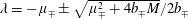 $\unicode[STIX]{x1D706}=-\unicode[STIX]{x1D707}_{\mp }\pm \sqrt{\unicode[STIX]{x1D707}_{\mp }^{2}+4b_{\mp }M}/2b_{\mp }$
.
$\unicode[STIX]{x1D706}=-\unicode[STIX]{x1D707}_{\mp }\pm \sqrt{\unicode[STIX]{x1D707}_{\mp }^{2}+4b_{\mp }M}/2b_{\mp }$
.
If oscillation dominates over dissipation the inequality
 $\unicode[STIX]{x1D707}_{\mp }^{2}\ll 4b_{\mp }M$
holds. Then roots of the characteristic equation (C 5) will be
$\unicode[STIX]{x1D707}_{\mp }^{2}\ll 4b_{\mp }M$
holds. Then roots of the characteristic equation (C 5) will be
 $$\begin{eqnarray}\unicode[STIX]{x1D706}=-{\displaystyle \frac{\unicode[STIX]{x1D707}_{\mp }}{2b_{\mp }}}\pm \sqrt{{\displaystyle \frac{M}{b_{\mp }}}}.\end{eqnarray}$$
This represents the equilibrium point (0, 0) that is a saddle point and hence unstable when
 $\unicode[STIX]{x1D707}_{\mp }^{2}\ll 4b_{\mp }M$
in both cases of low negative ion population (equilibrium dust charge negative) and high negative ion population (equilibrium dust charge positive).
$\unicode[STIX]{x1D707}_{\mp }^{2}\ll 4b_{\mp }M$
in both cases of low negative ion population (equilibrium dust charge negative) and high negative ion population (equilibrium dust charge positive).
Next, to study the stability of the equilibrium point
 $(2M/a_{\mp },0)$
we take the transformation
$(2M/a_{\mp },0)$
we take the transformation
 $$\begin{eqnarray}x=x^{\prime }+{\displaystyle \frac{2M}{a_{\mp }}},\quad y=y^{\prime }+0.\end{eqnarray}$$
Then deleting the prime symbol the dynamical system (C 2) and (C 3) can be written as,
 $$\begin{eqnarray}\left.\begin{array}{@{}c@{}}{\dot{x}}=y\\ {\dot{y}}=-{\displaystyle \frac{M}{b_{\mp }}}x-{\displaystyle \frac{\unicode[STIX]{x1D707}_{\mp }}{b_{\mp }}}y-{\displaystyle \frac{a_{\mp }}{2b_{\mp }}}x^{2},\end{array}\right\}\end{eqnarray}$$
which in matrix notation takes the form,
 $$\begin{eqnarray}\left(\begin{array}{@{}c@{}}{\dot{x}}\\ {\dot{y}}\end{array}\right)=\left(\begin{array}{@{}cc@{}}b_{11} & b_{12}\\ b_{21} & b_{22}\end{array}\right)\left(\begin{array}{@{}c@{}}x\\ y\end{array}\right)+\left(\begin{array}{@{}c@{}}f_{1}(x,y)\\ f_{2}(x,y)\end{array}\right).\end{eqnarray}$$
Here
 $b_{11}=0$
,
$b_{11}=0$
,
 $b_{12}=1$
,
$b_{12}=1$
,
 $b_{21}=-M/b_{\mp }$
,
$b_{21}=-M/b_{\mp }$
,
 $b_{22}=-\unicode[STIX]{x1D707}_{\mp }/b_{\mp }$
,
$b_{22}=-\unicode[STIX]{x1D707}_{\mp }/b_{\mp }$
,
 $f_{1}(x,y)=0$
,
$f_{1}(x,y)=0$
,
 $f_{2}(x,y)=a_{\mp }/2b_{\mp }x^{2}$
.
$f_{2}(x,y)=a_{\mp }/2b_{\mp }x^{2}$
.
The characteristic equation of the corresponding linear system in this case is,
 $$\begin{eqnarray}b_{\mp }\unicode[STIX]{x1D706}^{2}+\unicode[STIX]{x1D707}_{\mp }\unicode[STIX]{x1D706}+M=0,\end{eqnarray}$$
whose roots are
 $\unicode[STIX]{x1D706}=\unicode[STIX]{x1D6FC}_{\mp }\pm \text{i}\unicode[STIX]{x1D6FD}_{\mp }$
, where
$\unicode[STIX]{x1D706}=\unicode[STIX]{x1D6FC}_{\mp }\pm \text{i}\unicode[STIX]{x1D6FD}_{\mp }$
, where
 $$\begin{eqnarray}\unicode[STIX]{x1D6FC}_{\mp }=-{\displaystyle \frac{\unicode[STIX]{x1D707}_{\mp }}{2b_{\mp }}},\quad \unicode[STIX]{x1D6FD}_{\mp }=\sqrt{{\displaystyle \frac{M}{b_{\mp }}}}\end{eqnarray}$$
for
 $\unicode[STIX]{x1D707}_{\mp }^{2}<4b_{\mp }M$
. Here (C 11) shows that the critical point
$\unicode[STIX]{x1D707}_{\mp }^{2}<4b_{\mp }M$
. Here (C 11) shows that the critical point
 $(2M/a_{-},0)$
is a stable focus as
$(2M/a_{-},0)$
is a stable focus as
 $\unicode[STIX]{x1D707}_{-}>0$
when the negative ion population is low and equilibrium dust charge is negative. On the other hand
$\unicode[STIX]{x1D707}_{-}>0$
when the negative ion population is low and equilibrium dust charge is negative. On the other hand
 $(2M/a_{+},0)$
is an unstable focus as
$(2M/a_{+},0)$
is an unstable focus as
 $\unicode[STIX]{x1D707}_{+}<0$
when the negative ion population is high and equilibrium dust charge is positive.
$\unicode[STIX]{x1D707}_{+}<0$
when the negative ion population is high and equilibrium dust charge is positive.


