1. Introduction
Reverse osmosis (RO) systems play a key role in the water–energy–climate nexus due to their applications to seawater desalination and the treatment of municipal, agricultural and industrial wastewaters. RO removes solutes from a feed solution by pressurizing the feed and flowing it over a semi-permeable membrane sheet, as sketched in figure 1. The pressure difference across the membrane forces water through the membrane, while solutes are mostly blocked. Though modern RO is usually far more efficient than conventional distillation processes (Ghaffour, Missimer & Amy Reference Ghaffour, Missimer and Amy2013), it remains an energy-intensive process due to the large feed pressures (up to 80 bars) required to overcome the small membrane permeability and the large osmotic pressure difference across the membrane. To date, these energy demands have been primarily reduced by developing new membrane materials and energy recovery devices (Wang et al. Reference Wang, Dlamini, Mishra, Pendergast, Wong, Mamba, Freger, Verliefde and Hoek2014). Further improvements must address a phenomenon called concentration polarization, which is the accumulation of filtered solutes adjacent to the membrane surface, forming a concentration boundary layer, or ‘polarization layer’, as sketched in figure 1. This accumulation increases the transmembrane osmotic pressure and reduces the fraction of water recovered from the feed (Sablani et al. Reference Sablani, Goosen, Al-Belush and Wilf2001). It also leads to mineral scaling, which is the precipitation of salts onto the membrane surface. Mineral scaling reduces membrane life and increases downtime and maintenance costs (Lyster et al. Reference Lyster, Au, Rallo, Giralt and Cohen2009). It also contributes to biofouling by driving nutrients to the membrane surface (Mansouri, Harrisson & Chen Reference Mansouri, Harrisson and Chen2010). More broadly, concentration polarization is a challenge in nearly all membrane filtration processes, including ultrafiltration processes, where it leads to the formation of gel layers, and thermally driven membrane distillation processes (Lou et al. Reference Lou, Vanneste, Decaluwe, Cath and Tilton2019, Reference Lou, Johnston, Cath, Martinand and Tilton2021) where it impedes the treatment of high-concentration waste brine.

Figure 1. Sketch demonstrating concentration polarization in a plate-and-frame RO system.
Current efforts to decrease concentration polarization often focus on the hydrodynamic role of feed spacers (Ahmad & Lau Reference Ahmad and Lau2006). Feed spacers are a mesh-like material placed in the feed channel to support fragile membrane sheets and provide room for feed flow tangential to the membrane. For sufficiently large feed flow rates, the filaments of these spacers also generate unsteady vortical flow structures due to a wake instability similar to the von Kármán vortex street. Experimental and numerical works suggest that these vortical structures increase the transmembrane flow by stirring and attenuating concentration boundary layers (refer to the works of Haidari, Heijman & van der Meer Reference Haidari, Heijman and van der Meer2016, Reference Haidari, Heijman and van der Meer2018a,Reference Haidari, Heijman and van der Meerb, for reviews). Despite the considerable work to date, spacers are still primarily designed using experience and trial and error. Due to their complicated geometry, our knowledge of the flow regime in RO systems with feed spacers remains inadequate. Meanwhile, the more fundamental question of how vortical structures might interact with concentration polarization is itself poorly understood.
The present study investigates an aspect of this latter question by considering RO in the Taylor–Couette cell sketched in figure 2(a). In the annular gap between two concentric cylinders, a feed solution composed of a solvent and a solute is set in motion by the rotation of the inner cylinder. There is no applied pressure gradient in the axial direction, and contrary to traditional RO systems, there is no mean axial flow. Both cylinders are semi-permeable membranes through which solvent can flow, while the solute is retained in the annular gap. The inner membrane surrounds a cavity filled with pure solvent maintained at a desired constant pressure  $P_{{in}}$. The region outside the outer membrane is similarly filled with solvent maintained at the constant pressure
  $P_{{out}}$. Note that figure 2(a) only shows the fluid in the annular gap. Applying a radial pressure difference
  $\Delta P=P_{{in}}-P_{{out}}$ drives a radial throughflow of solvent across both cylindrical membranes and the gap. The solute advected by the radial throughflow forms a concentration boundary layer at the cylinder through which the solvent exits the gap.

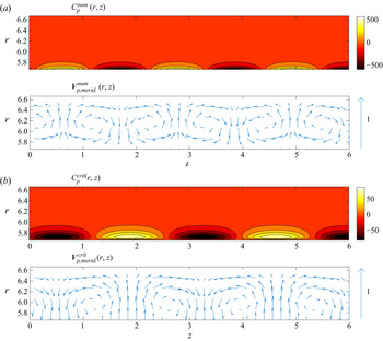
Figure 2. (a) Sketch of the base-state flow and concentration field in a Taylor–Couette cell with two semi-permeable cylinders and a superimposed radial inflow. (b) Sketch of the counter-rotating Taylor vortices (the blue online toroidal streamtubes), the outward and inward jets which (the black arrows) advect the concentration boundary layer to form zones of alternate accumulation and depletion of solute, shown in the planform above.
We show that, below a critical rotation rate of the inner cylinder, the flow fields in this set-up admit a simple steady analytical solution, as shown in figure 2(a). Beyond that rotation rate, toroidal Taylor vortices appear as sketched in figure 2(b). These counter-rotating vortices form alternating outward and inward radial jets. These jets stir the concentration boundary layer and form alternating regions of solute accumulation and depletion on the membrane surface. Osmosis then acts to dilute regions of solute accumulation and concentrate regions of solute depletion. This occurs by a reduction of the outgoing transmembrane flow in regions of accumulation and an increase of the transmembrane flow in regions of depletion. These variations of the transmembrane flow in turn likely retroact on the vortices. Assessing this mechanism is the goal of the present work. More specifically, we focus on the question of whether concentration polarization and osmotic pressure act in favour or against the formation of vortices. The subsequent question of whether vortices increase or decrease the average transmembrane flow is left for future work.
This Taylor–Couette configuration provides a unique ‘test bed’ with which we can control, observe and study the interactions between vortices, concentration polarization and osmotic pressure. First, the characteristics of the concentration polarization layer can be controlled by imposing the radial flow, independently of the azimuthal flow driven by the rotation of the inner cylinder. Second, the appearance of vortices due to a centrifugal instability can be easily controlled by setting the rotation rate of the inner cylinder. These centrifugal instabilities and their critical conditions are well studied and understood and we show that our specific configuration also admits a simple analytical solution for the base state, which permits an analytical stability analysis and a parametric study of the vortices. Finally, the straightforward geometry allows complementary direct numerical simulations using high-order spectral methods.
Our particular configuration is of limited practical use for filtration, because the amount of solvent extracted through one cylinder is balanced by that entering through the other. In industry, rotating filtration processes based on Taylor–Couette cells have a stationary impermeable outer cylinder and a rotating semi-permeable inner cylinder. Feed is pumped axially through the gap while solvent exits the inner cylinder. Although this mode of filtration has niche applications in separating blood plasma from cells, its poor membrane–surface to volume ratio and complicated moving parts make it unrealistic for industrial RO (Hallström & Lopez-Leiva Reference Hallström and Lopez-Leiva1978; Margaritis & Wilke Reference Margaritis and Wilke1978; Kroner & Nissinen Reference Kroner and Nissinen1988; Ohashi et al. Reference Ohashi, Tashiro, Kushiya, Matsumoto, Yoshida, Endo, Horio, Osawa and Sakai1988; Beaudoin & Jaffrin Reference Beaudoin and Jaffrin1989; Belfort et al. Reference Belfort, Mikulasek, Pimbley and Chung1993a,Reference Belfort, Pimbley, Greiner and Chungb; Lueptow & Hajiloo Reference Lueptow and Hajiloo1995; Schwille, Mitra & Lueptow Reference Schwille, Mitra and Lueptow2002). Taylor–Couette flow and its various regimes have been widely studied experimentally, numerically and analytically (see discussions and references in Taylor Reference Taylor1923; Coles Reference Coles1965; Davey, DiPrima & Stuart Reference Davey, DiPrima and Stuart1968; Cole Reference Cole1976; Marcus Reference Marcus1984; Andereck, Liu & Swinney Reference Andereck, Liu and Swinney1986; Koshmieder Reference Koshmieder1993; Bilson & Bremhorst Reference Bilson and Bremhorst2007; Ostilla-Monico et al. Reference Ostilla-Monico, van der Poel, Verzicco, Grossmann and Lohse2014, among many others). The current work considers cases where the outer cylinder remains stationary. We also focus on the initial transition from steady flow to toroidal vortices, the stability of which is known to be retrieved by linear stability analysis. The stability of a Taylor–Couette cell filled with pure solvent, with a stationary outer cylinder and a superimposed radial flow through both cylinders was first considered by Bahl (Reference Bahl1970). For narrow gaps, linear stability analyses (Min & Lueptow Reference Min and Lueptow1994; Martinand, Serre & Lueptow Reference Martinand, Serre and Lueptow2017) and direct numerical simulations (Serre, Sprague & Lueptow Reference Serre, Sprague and Lueptow2008) show that a radial inflow or strong radial outflow have a stabilizing effect, while a small radial outflow has a slightly destabilizing effect for the first transition from non-vortical to vortical flows. Extending the analysis to large gaps, Martinand et al. (Reference Martinand, Serre and Lueptow2017) found that a strong radial outflow can select pairs of counter-propagating helical vortices, and a strong radial inflow tends to squeeze the vortices against the inner cylinder and dramatically shrink their cross-section in a meridional plane. Weakly nonlinear analyses and numerical simulations (Martinand et al. Reference Martinand, Serre and Lueptow2017) also found that a strong radial outflow or inflow modified the usual supercritical transition to a subcritical transition, exhibiting a hysteresis cycle.
To date, the above analytical and numerical results have all been obtained by imposing a prescribed radial velocity to the base flow, while simultaneously prescribing a no-penetration condition, i.e. a zero radial velocity, to the instabilities. This assumption neglects the potential for flow instabilities to penetrate into the permeable surfaces, which has been shown to destabilize channel and boundary layer flows.
The mixing and transport properties of Taylor vortices have been studied both from a fundamental point of view (Akonur & Lueptow Reference Akonur and Lueptow2002; Nemri et al. Reference Nemri, Climent, Charton, Lanoe and Ode2013) and for practical applications (Miyashita & Senna Reference Miyashita and Senna1993; Giordano, Giordano & Cooney Reference Giordano, Giordano and Cooney2000a; Giordano et al. Reference Giordano, Giordano, Prazeres and Cooney2000b; Aljishi et al. Reference Aljishi, Ruo, Park, Nasser, Kim and Joo2013). Nevertheless, no studies to date have considered the boundary conditions associated with the rejection of the solute at a membrane and the build-up of a concentration boundary layer together with osmotic pressure. The coupling between transmembrane flow and osmotic pressure has been modelled and studied in boundary layers or channel flows (Haldenwang et al. Reference Haldenwang, Guichardon, Chiavassa and Ibaseta2010; Lopes et al. Reference Lopes, Bernales, Ibaseta, Guichardon and Haldenwang2012; Bernales et al. Reference Bernales, Haldenwang, Guichardon and Ibaseta2017). But these works have focused on laminar flows within the Prandtl approximation, thus excluding the possibility of vortical flows.
The article is organized as follows. Section 2 presents the geometry, governing equations and base state. Section 3 describes the linear stability analysis and the numerical methods. Section 4 first demonstrates the impact of osmotic pressure on centrifugal instabilities by presenting converging numerical and analytical results (§ 4.1) then quantitatively assesses over a relevant parameter space the magnitude of this impact on the critical conditions (§ 4.2) and spatial structures (§ 4.3) of the instabilities. Section 5 further explains how the semi-permeable membrane and the related velocity and concentration boundary conditions generate this effect. Section 6 sums up our results by expressing analytically the range of parameters over which osmosis impacts the instabilities and the magnitude of this impact as a function of the radius ratio only. Section 7 discusses the interest and limitations of the set-up and presents possible future works.
2. Geometry, governing equations and base state
We consider a Taylor–Couette cell with a stationary outer cylinder of radius  $r_{2}$, and a concentric inner cylinder of radius
  $r_{1}$. The inner cylinder rotates about its longitudinal axis with constant angular velocity
  $\varOmega$, as sketched in figure 2. The flow of interest occurs in the annular gap
  $r_{1} \le r \le r_{2}$, which is filled with an incompressible Newtonian solution composed of a solvent (water) and solute. Hereinafter, we use cylindrical coordinates
  $\boldsymbol {x}=(r,\theta,z)$, in which the fluid velocity vector is denoted
  $\boldsymbol {V}=(U,V,W)^{t}$, where
  $U$,
$U$,  $V$ and
  $W$ are the radial, azimuthal and axial components, respectively. The fluid pressure is denoted
  $P$. The concentration is denoted
  $C$, and expressed in
  ${\rm mol}\,{\rm m}^{-3}$.
The inner and outer cylinders are both semi-permeable membranes of thickness  $h$, through which only the solvent can flow. The inner membrane surrounds a cavity (
 $r< r_{1}-h$) filled with solvent maintained at constant pressure
  $P_{{in}}$. Similarly, the region beyond the outer membrane (
 $r>r_{2}+h$) is filled with solvent maintained at constant pressure
  $P_{{out}}$. The pressure difference between these cavities,
 \begin{equation} \Delta P=P_{{in}}-P_{{out}}, \end{equation}
drives radial flow through the annular gap. A positive  $\Delta P$ drives flow in the positive radial direction, with solvent entering the inner cylinder and leaving the outer cylinder. This causes solute accumulation at the outer cylinder. A negative
  $\Delta P$ drives flow in the negative radial direction, causing solutes to accumulate at the inner cylinder.
Both membrane surfaces satisfy the no-slip condition for the tangential velocity components  $V$ and
  $W$
$W$
 \begin{equation} \left. V\right|_{r=r_{1}}=\varOmega r_{1}, \quad \left.W\right|_{r=r_{1}}=\left.V\right|_{r=r_{2}} =\left.W\right|_{r=r_{2}}=0. \end{equation}
Radial solvent flow through the inner membrane satisfies a boundary condition involving the transmembrane pressure difference and transmembrane concentration difference in the form of an osmotic pressure given by van't Hoff's law
 \begin{equation} \left.U\right|_{r=r_{1}}=K\left(\left.P_{{in}}-P\right|_{r=r_{1}} +\left.RTC\right|_{r=r_{1}}\right), \end{equation}
where  $K$ is the membrane permeance to water in the wall-normal direction, defined as the transmembrane velocity of solvent per unit pressure difference,
  $R$ is the ideal gas constant and
  $T$ is the fluid temperature, assumed constant. Similarly, solvent flow through the outer cylinder satisfies
 \begin{equation} \left. U\right|_{r=r_{2}}={-}K\left(P_{{out}}-\left. P\right|_{r=r_{2}}+\left.RTC\right|_{r=r_{2}}\right). \end{equation}
Flows over permeable surfaces may have a non-zero tangential velocity at the surface due to momentum transfer to the fluid within the porous material (see Beavers & Joseph Reference Beavers and Joseph1967). This tangential velocity is important when a streamwise pressure gradient drives a streamwise flow within the porous material. In filtration flow, the no-slip assumption (2.2a,b) is reasonable, because the permeability (or the permeance in our case) is very small, and the membrane very thin. Consequently, the transmembrane pressure gradient, i.e. the transmembrane pressure difference over the membrane thickness, necessary to drive even a small transmembrane velocity is several orders-of-magnitude higher than any pressure gradient tangent to the wall. For systems in which the no-slip assumption is invalid, porous surfaces should be modelled using appropriate momentum transfer condition (see Beavers & Joseph Reference Beavers and Joseph1967), but to the best of our knowledge, such conditions have never been numerically and/or analytically implemented and assessed in filtration set-ups.
The absence of any solute flux through the inner and outer cylinders requires radial advection and diffusion of solutes to sum to zero at  $r_{1}$ and
  $r_{2}$,
 \begin{equation} \left[UC-{\mathcal{D}}\frac{\partial C}{\partial r}\right]_{r=r_{1}}=\left[UC-{\mathcal{D}}\frac{\partial C}{\partial r}\right]_{r=r_{2}}=0, \end{equation}
where  ${\mathcal {D}}$ is the solute molecular diffusivity. It is worth stressing here that the no-flux boundary condition (2.5) has a nonlinear term,
  $UC$.
$UC$.
There is no applied axial pressure gradient and, equivalently, no net axial fluid flow. As a consequence, the mass flow rate entering the gap through one of the cylinders balances that leaving through the other, leading to
 \begin{equation} r_{1}\left\langle U\right\rangle_{r_{1}}=r_{2}\left\langle U\right\rangle_{r_{2}}, \end{equation}
where  $\left \langle U\right \rangle _{r_i}$ denote the radial velocities averaged over the inner (
 $i=1$) and outer (
 $i=2$) cylinders. Due to this balance in radial mass flow rates, solute accumulation at one cylinder is balanced by depletion at the other, such that the solute concentration
  $C_0$ averaged over the full domain remains constant. This configuration allows us to control all the physical mechanisms of interest in this study, i.e. the build up of a concentration boundary layer, the coupling between the osmotic pressure and transmembrane flow, and the driving of hydrodynamic instabilities.
2.1. Non-dimensional parameters and equations
Fluid flow and solute transport in the gap are governed by the incompressible continuity, Navier–Stokes and advection–diffusion equations. These are non-dimensionalized using the gap width  $d = r_{2} - r_{1}$ for the characteristic length,
  $\nu /d$ for the characteristic velocity,
  $d^2/\nu$ for the characteristic time,
  $\rho {\nu ^2}/d^2$ for the characteristic pressure and the average concentration
  $C_{0}$ for the characteristic concentration, where
  $\rho$ is the fluid density and
  $\nu$ its kinematic viscosity. Hereinafter, all expressions are non-dimensional, unless otherwise stated. The governing equations may be expressed as
 \begin{equation} \left. \begin{aligned} & \displaystyle \boldsymbol{\nabla}\boldsymbol{\cdot}\boldsymbol{V}={0} ,\\ & \displaystyle \frac{\partial \boldsymbol{V}}{\partial t} +\left(\boldsymbol{V}\boldsymbol{\cdot}\boldsymbol{\nabla}\right)\boldsymbol{V}={-}\boldsymbol{\nabla}{P}+\nabla^2\boldsymbol{V} ,\\ & \displaystyle \frac{\partial {C}}{\partial t}+\boldsymbol{V}\boldsymbol{\cdot}\boldsymbol{\nabla}{C}= \frac{1}{{Sc}}\nabla^2{C} , \end{aligned} \right\} \end{equation}
where  ${Sc} = {\nu }/{\mathcal {D}}$ is the Schmidt number. Boundary conditions are now expressed at the non-dimensional inner and outer radii
  $r_{1}=\eta /(1-\eta )$ and
  $r_{2}=1/(1-\eta )$, respectively. The boundary conditions for the tangential velocity components can be expressed as
 \begin{equation} \left. V\right|_{r=r_{1}} = {Ta}, \quad \left.W\right|_{r=r_{1}} = \left.V\right|_{r=r_{2}} = \left.W\right|_{r=r_{2}} = 0, \end{equation}
where  ${Ta} = r_{1} \varOmega d/\nu$ is the Taylor number. The boundary conditions for
  $U$ and
  $C$ at the cylinder are written as
 \begin{equation} \left. \begin{aligned} \displaystyle \left.U\right|_{r=r_{1}}=\sigma \left(P_{{in}}-\left.P\right|_{r=r_{1}}\right)+\chi \left.C\right|_{r=r_{1}},\\ \displaystyle \left. U\right|_{r=r_{2}}={-}\sigma \left(P_{{out}}-\left. P\right|_{r=r_{2}}\right)-\chi \left.C\right|_{r=r_{2}}, \end{aligned} \right\} \end{equation}
 \begin{equation} \left[{Sc} \,UC - \frac{\partial C} {\partial r} \right]_{r=r_{1}}= \left[ {Sc} \,UC - \frac{\partial C} {\partial r} \right]_{r=r_{2}}=0. \end{equation}
The semi-permeable nature of the membrane and its permeance  $K$ manifest through two independent non-dimensional coefficients in boundary conditions (2.9a): the velocity–pressure coupling coefficient
  $\sigma = K\rho \nu /d$ and the velocity–concentration coupling coefficient
  $\chi = {K R T d\,C_{0}}/{\nu }$. Lastly, the averaged transmembrane velocities are expressed in terms of the Reynolds number
 \begin{equation} {Re} = \frac{r_{1}\left\langle U\right\rangle_{r_{1}}}{\nu} = \frac{r_{2}\left\langle U\right\rangle_{r_{2}}}{\nu}. \end{equation}
 Although this set-up is not commonly used in industrial RO or nanofiltration devices, we nonetheless establish the ranges of the non-dimensional parameters that would prevail in a RO Taylor–Couette cell with semi-permeable cylinders and filled with seawater. In typical seawater plate-and-frame RO systems, the transmembrane velocity is of order  $10^{-6}\,\textrm {m}\,\textrm {s}^{-1}$ for operating pressure ranging from
  $5$ to
  $8$ MPa, with the osmotic pressure being around
  $3$ MPa. The permeance
  $K$ of these membranes is of order
  $10^{-13}$ to
  $10^{-12}\,\textrm {m}\,\textrm {s}^{-1}\,\textrm {Pa}^{-1}$ (see table 1 in van Wagner et al. Reference van Wagner, Sagle, Sharma and Freeman2009, for examples of commercial RO membranes). Assuming arbitrarily the radii
  $r_{1}$ and
  $r_{2}$ are of order
  $10^{-2}$ to
  $10^{-1}$ m, and the gap width
  $d$ is of order
  $10^{-3}$ to
  $10^{-2}$ m, produces velocity–pressure coupling coefficients and Reynolds numbers ranging between
  $10^{-14}<\sigma <10^{-12}$ and
  $10^{-2}<{Re}<10^{-1}$, respectively. Assuming seawater at
  $25\,^{\circ }\textrm {C}$, with an average salt concentration
  $C_0\approx 10^{3}\,\textrm {mol}\,\textrm {m}^{-3}$, produces velocity–concentration coupling coefficients ranging between
  $10^{-3}<\chi <10^{-1}$. Considering that
  ${\mathcal {D}}$ for monovalent ions such as Na
 $^{+}$ and Cl
 $^{-}$ is of order
  $10^{-9}\,\textrm {m}^2\,\textrm {s}^{-1}$, the Schmidt number is of order
  $10^{3}$. Typical transitional Taylor numbers
  ${Ta}\sim 100$ then correspond to rotation rates
  $\varOmega$ ranging from
  $10^{-1}$ to
  $10\,\textrm {rad}\,\textrm {s}^{-1}$.
2.2. Steady base state
Equations (2.7)–(2.9) admit a steady, axially and azimuthally invariant base state  $[\boldsymbol {V}_b(r),\,P_b(r),\,C_b(r)]$, the expression of which is given in Appendix A. These velocity and pressure fields are parameterized by
  ${Ta}$ and
  ${Re}$ solely. Positive values of
  ${Re}$ produce a radial velocity
  $U_b>0$ flowing outwards, while
  ${Re}<0$ produces radial velocities
  $U_b<0$ flowing inwards, as seen in figure 3(a) for
  ${Re}=-0.1$. By writing the base state in this form, we apply the Reynolds number
  ${Re}$ directly, and then compute the necessary operating pressure (2.1) from boundary conditions (2.9a),
 \begin{equation} \Delta P=P_b(r_{1})-P_b(r_{2}) + \frac{\chi}{\sigma}\left[ C_b(r_{2})- C_b(r_{1})\right] + \frac{1}{\sigma}\left[ U_b(r_{2}) + U_b(r_{1})\right]. \end{equation}
Figure 3. (a) Radial velocity of the base state  $U_b(r)$ for radius ratio
  $\eta =0.85$ and radial inflow
  ${Re}=-0.1$. (b) Concentration field of the base state
  $C_b(r)$ for radius ratio
  $\eta =0.85$ a radial inflow with Péclet number
  ${Pe}={Re}\,{Sc}=-20$ (light grey, green online) and
  ${Pe}={Re}\,{Sc}=-100$ (dark grey, blue online). The vertical dashed (blue online) line materializes the polarization layer thickness
  $\delta$ as computed from (2.15) for
  ${Pe}=-100$.
To further interpret the concentration boundary layer, the base state  $C_b$ in (A4) can be re-expressed in terms of the radius ratio
  $\eta =r_{1}/r_{2}$ and the Péclet number associated with the radial transmembrane flow
  ${Pe}={Re}\,{Sc}$
 \begin{equation} C_b(r)=\frac{{Pe}+2}{2}\frac{1-\eta^2}{1-\eta^{{Pe}+2}}\left(1-\eta\right)^{{Pe}}r^{{Pe}}\quad\text{for}\ {Pe}\neq{-}2. \end{equation}
 Figure 3(b) shows two examples of  $C_b$ when
  $\eta =0.85$ with Péclet numbers
  ${Pe}=-20$ (light grey, green online) and
  ${Pe}=-100$ (dark grey, blue online). As
  ${Pe}$ increases in absolute value, whether by increasing the Reynolds or the Schmidt numbers, the solute accumulates in an increasingly thin boundary layer near the inner membrane. Simultaneously, pure solvent entering through the outer cylinder depletes the solute concentration outside the polarization layer. To characterize the base-state polarization layer, we first compute the maximum concentration
  $C_{b,{max}}$ (shown as dots in figure 3), which occurs on the membrane surface. We then define the polarization layer thickness
  $\delta$ as the radial distance from the membrane where the concentration is
  $0.05C_{b,{max}}$. Depending on the direction of the radial flow,
  $C_{b,{max}}$ is obtained from (2.12) as
 \begin{equation} C_{b,{max}} = \left\{ \begin{array}{@{}ll} \displaystyle C_b(r_{1}) = \dfrac{-({Pe}+2)}{2} \, \dfrac{1-\eta^{2}}{1-\eta^{-({Pe} + 2)}}\dfrac{1}{\eta^2}, & \text{for} \ {Pe} < 0,\\ \displaystyle C_b(r_{2}) = \dfrac{{Pe}+2}{2} \, \dfrac{1 - \eta^{2}}{1-\eta^{{Pe} + 2}}, & \text{for} \ {Pe} > 0, \end{array} \right. \end{equation}
and, combined with (2.12), leads to
 \begin{equation} \delta = \left\{ \begin{array}{@{}ll} \displaystyle(0.05^{1/{Pe}}-1)\dfrac{\eta}{1-\eta}, & \text{for} \ {Pe} < 0,\\ \displaystyle(1-0.05^{1/{Pe}})\dfrac{1}{1-\eta}, & \text{for} \ {Pe} > 0. \end{array}\right. \end{equation}
For large Péclet numbers (in absolute value), the boundary layer thickness can be approximated by
 \begin{equation} \delta\approx \left\{ \begin{array}{@{}ll} \displaystyle \dfrac{\log(20)}{-{Pe}}\dfrac{\eta}{1-\eta}, & \text{for} \ {Pe} < 0,\\ \displaystyle \dfrac{\log(20)}{{Pe}}\dfrac{1}{1-\eta}, & \text{for} \ {Pe} > 0, \end{array} \right. \end{equation}
and is inversely proportional to the Péclet number. Figure 4 shows  $C_{b,{max}}$ and
  $\delta$ as functions of the radius ratio
  $\eta$ and Péclet number
  ${Pe}$, where
  ${Pe}<0$ represents radial inflow and
  ${Pe}>0$ represents radial outflow. Maximum non-dimensional concentrations beyond
  $10^3$ are not depicted, because these would likely trigger solute precipitation and call the governing equations into question. Non-dimensional boundary layer thicknesses above
  $1$ are not shown because this would correspond to layers larger than the gap. For
  $\delta >1$, one can assume that no boundary layer forms. As expected, increasing the magnitude of the Péclet number reduces the boundary layer thickness
  $\delta$ and increases the maximum concentration
  $C_{b,{max}}$. Decreasing the radius ratio
  $\eta$, by reducing the radii
  $r_{1}$ and
  $r_{2}$, increases the magnitude of the velocities
  $U_b(r_{1})$ and
  $U_b(r_{2})$ for a prescribed Péclet number. It thus reduces the boundary layer thickness
  $\delta$ and increases the maximum concentration
  $C_{b,{max}}$. Note that for a given Péclet number, the magnitude of the radial velocity through the inner cylinder always exceeds that through the outer, because
  $U_b(r_{1}) = U_b(r_{2})/\eta$. Consequently, in figure 4(a), the solute concentration on the inner cylinder is greater than that on the outer cylinder. Accordingly, in figure 4(b), the boundary layer at the inner cylinder is thinner than that on the outer cylinder.

Figure 4. (a) Maximum of the concentration field  $C_{b,{max}}$ (in log scale) as a function of the radius ratio
  $\eta$ and Péclet number
  ${Pe}={Re}\,{Sc}$ (in log scale). (b) Boundary layer thickness
  $\delta$ (in log scale) as a function of the radius ratio
  $\eta$ and Péclet number
  ${Pe}={Re}\,{Sc}$ (in log scale). Note the uncommon
  ${Pe}$-axis merging negative and positive values of this parameter to account for radial in- and outflows, and the resulting discontinuities of the surfaces. Note also the reversed
  $\eta$-axes in both figures.
The base state ((A1a,b)–(A4)) does not present any dependence on the velocity– concentration coupling coefficient  $\chi$ and velocity–pressure coupling coefficient
  $\sigma$, as these parameters only affect the operating pressure (2.11). This operating pressure is of major practical importance because it imposes the non-dimensional power per unit axial length needed to drive the fluid across the Taylor–Couette cell:
  ${\mathcal {P}}=2{\rm \pi} {Re}\Delta P$. The impact of system design and operating conditions on
  $\Delta P$ can be understood by investigating each term in expression (2.11), repeated below for convenience
 \begin{equation} \Delta P=P_b(r_{1})-P_b(r_{2}) + \frac{\chi}{\sigma}[ C_b(r_{2})- C_b(r_{1})] + \frac{1}{\sigma}[ U_b(r_{2}) + U_b(r_{1})]. \end{equation}
The first term  $P_b(r_{1})-P_b(r_{2})$ is due to hydrodynamics and combines a contribution due to the curvature of the azimuthal flow, scaling with
  ${Ta}^2$, and a contribution due to the radial flow, scaling with
  ${Re}^2$, both up to multiplicative functions of
  $\eta$. The next term
 \begin{equation} \frac{\chi}{\sigma}\left[C_b(r_{2})-C_b(r_{1})\right]=\frac{\chi\left({Pe}+2\right)}{2\sigma}\frac{1-\eta^2}{1-\eta^{{Pe}+2}}(1-\eta^{{Pe}}), \end{equation}
is due to the osmotic pressure. For large Péclet numbers (in absolute value), it mostly scales with  $\chi {Pe}\,\sigma ^{-1}=\chi {Re}\,{Sc}\,\sigma ^{-1}$, up to a multiplicative function of
  $\eta$. The last term
 \begin{equation} \frac{1}{\sigma}\left[U_b(r_{2})+U_b(r_{1})\right]=\frac{{Re}}{\sigma}\frac{1-\eta^2}{\eta}, \end{equation}
is due to the transmembrane flow of solvent and scales with  ${Re}\,\sigma ^{-1}$, up to a multiplicative function of
  $\eta$. Typical membrane filtration conditions present very small
  $\sigma$, such that the hydrodynamic term in the operating pressure (2.11) is negligible compared with the two next terms, i.e. the operating pressure is mostly imposed by the membrane permeance and osmotic pressure. Neglecting the hydrodynamic terms leads to the approximation
 \begin{equation} \frac{\sigma\Delta P}{{Re}}\approx\frac{1-\eta^2}{\eta}\left(1+\frac{\chi\, {Sc}\left({Pe}+2\right)}{2{Pe}}\eta\frac{1-\eta^{{Pe}}}{1-\eta^{{Pe}+2}}\right), \end{equation}
depicted in figure 5 for narrow ( $\eta =0.85$) and wide (
 $\eta =0.25$) gaps. For narrow gaps, this operating pressure is almost independent of the Péclet number. For wide gaps, the operating pressure becomes substantially stronger for inflows than for outflows, due to the strong discrepancy between the transmembrane velocities at the inner and outer cylinders.

Figure 5. Reduced operating pressure  $\sigma \Delta P/{Re}$ as a function of
  $\chi \,{Sc}$ and
  ${Pe}={Re}\,{Sc}$, for (a)
  $\eta =0.85$ and (b)
  $\eta =0.25$. All quantities are in log scale and note the uncommon
  ${Pe}$-axis merging positive and negative values of this parameter to account for out- and inflows and the resulting discontinuities of the surfaces.
3. Analytical and numerical methods
We explore the appearance of vortical flow structures and their coupling with concentration polarization by performing a linear stability analysis of the base state. We also perform complementary direct numerical simulations of the complete flow fields.
3.1. Linear stability analysis
The stability analysis decomposes the flow fields into the sum of the base state  $[\boldsymbol {V}_{b},\,{P}_{b},\,{C}_{b}]$ and small perturbations
  $[\boldsymbol {V}_{p}(\boldsymbol {x},t),\,{P}_{p}(\boldsymbol {x},t),\,{C}_{p}(\boldsymbol {x},t)]$. Linearizing equations (2.7) about the base state produces the following evolution equations for the small perturbation,
 \begin{equation} \left. \begin{aligned} & \displaystyle \boldsymbol{\nabla}\boldsymbol{\cdot}\boldsymbol{V}_{p}={0}\, ,\\ & \displaystyle \frac{\partial \boldsymbol{V}_{p}}{\partial t}+\boldsymbol{V}_{b}\boldsymbol{\cdot}\boldsymbol{\nabla}\boldsymbol{V}_{p} + \boldsymbol{V}_{p}\boldsymbol{\cdot}\boldsymbol{\nabla}\boldsymbol{V}_{b} ={-}\boldsymbol{\nabla}{P_{p}}+\nabla^2\boldsymbol{V}_{p} ,\\ & \displaystyle \frac{\partial {C_{p}}}{\partial t}+\,\boldsymbol{V}_{b}\boldsymbol{\cdot}\boldsymbol{\nabla}{C_{p}} +\boldsymbol{V}_{p}\boldsymbol{\cdot}\boldsymbol{\nabla}{C_{b}}= \frac{1}{{Sc}}\nabla^2{C_{p}}. \end{aligned} \right\} \end{equation}
The linearization of boundary conditions (2.9) produces
 \begin{equation} \left.V_{p}\right|_{r=r_{i}} = \left.W_{p}\right|_{r=r_{i}} = 0, \end{equation}
 \begin{equation} \displaystyle\left. U_{p}\right|_{r=r_{i}}={\mp} \left[\sigma P_{p}-\chi C_{p}\right]_{r=r_{i}}, \end{equation}
 \begin{equation} \left[ U_{p} C_{b} + U_{b} C_{p} -\frac{1}{{Sc}}\frac{\partial C_{p}} {\partial r} \right]_{r=r_i}= 0, \end{equation}
where  $r_i=r_{1}$ or
  $r_{2}$, and the negative (positive) sign in condition (3.2b) is used when
  $r=r_{1}$ (
 $r=r_{2}$). Note that the terms
  $U_pC_b$ and
  $U_bC_p$ in the no-flux condition (3.2c) arise from the linearization of the solute advection term
  $UC$ in condition (2.5).
Our stability analysis considers perturbations of the form
 \begin{equation} \left[\boldsymbol{V}_{p}(\boldsymbol{x},t),\,{P}_{p}(\boldsymbol{x},t),\,{C}_{p}(\boldsymbol{x},t)\right] = [\boldsymbol{v}_{p}(r),\,p_{p}(r),\,c_{p}(r)] \exp (\mathrm{i} k z + \mathrm{i} n \theta + st), \end{equation}
where  $k$ and
  $n$ are the axial and azimuthal wavenumbers, respectively,
  $s$ is the growth rate and
  $[\boldsymbol {v}_{p}(r),\,p_{p}(r),\,c_{p}(r)]$ are radial profiles, describing the variation of the perturbation structures in the radial direction. Substituting form (3.3) into the linearized equations (3.1)–(3.2) produces a generalized eigenvalue problem
 \begin{equation} {\mathcal{A}}[\boldsymbol{v}_{p},\,p_{p},\,c_{p}] ={-} s {\mathcal{B}} [\boldsymbol{v}_{p},\,p_{p},\,c_{p}], \end{equation}
for which  $s$ and
  $[\boldsymbol {v}_{p},\,p_{p},\,c_{p}]$ are the eigenvalues and eigenvectors, respectively. The differential operators
  ${\mathcal {A}}$ and
  ${\mathcal {B}}$ are given in Appendix B. The radial profiles satisfy the boundary conditions
 \begin{equation} v_{p}(r_{i}) =w_{p}(r_{i}) = 0, \end{equation}
 \begin{equation} u_{p}(r_{i})={\mp} \left[\sigma p_{p}\left(r_{i}\right) - \chi c_{p}\left(r_{i}\right)\right], \end{equation}
 \begin{equation} u_{p}(r_{i}) C_{b}(r_{i}) + U_{b}(r_{i}) c_{p}(r_{i}) - \frac{1}{{Sc}}\frac{d c_{p}} {d r}(r_{i}) = 0, \end{equation}
where, again,  $r_i=r_{1}$ or
  $r_{2}$, and the negative sign in condition (3.5b) is used when
  $r=r_{1}$.
The eigenvalue problem is solved using a standard spectral collocation method with a typical resolution of  $72$ Chebyshev polynomials in the radial direction. Newton–Raphson methods previously explained in Martinand, Serre & Lueptow (Reference Martinand, Serre and Lueptow2009) are used to determine the critical conditions of the most unstable mode. This yields the critical Taylor number
  $Ta^{{crit}}$ above which the real part of a first eigenvalue
  $s$, associated with the eigenmode
  $[\boldsymbol {v}_{p}^{{crit}},\,p_{p}^{{crit}},\,c_{p}^{{crit}}]$ with axial wavenumber
  $k^{{crit}}$ and azimuthal wavenumber
  $n^{{crit}}$, becomes positive.
3.2. Direct numerical simulations
We perform axisymmetric direct numerical simulations (DNS) of (2.7)–(2.9) using an in-house pseudo-spectral code previously detailed in Tilton et al. (Reference Tilton, Serre, Martinand and Lueptow2014). The code has been successfully used to simulate tubular membrane filtration systems (Tilton et al. Reference Tilton, Martinand, Serre and Lueptow2012), and steady (Tilton et al. Reference Tilton, Martinand, Serre and Lueptow2010) and unsteady (Tilton & Martinand Reference Tilton and Martinand2018) flows in Taylor–Couette–Poiseuille cells with permeable inner cylinders and pure solvent, and has been modified to include the resolution of the scalar equation and boundary conditions (2.9). The code discretizes the radial and axial directions using Chebyshev polynomials, and uses a second-order semi-implicit temporal scheme suggested by Vanel, Peyret & Bontoux (Reference Vanel, Peyret and Bontoux1986). The pressure solver is based on the projection method introduced in Raspo et al. (Reference Raspo, Hughes, Serre, Randriamampianina and Bontoux2002) and extended in Tilton et al. (Reference Tilton, Serre, Martinand and Lueptow2014) to satisfy the velocity–pressure and velocity–concentration couplings on the semi-permeable membranes. We simulate a domain of non-dimensional axial length  $L=20$ with
  $36$ and
  $148$ collocation points in the radial and axial directions, respectively. Spatial convergence is confirmed by monitoring the Chebyshev expansion coefficients. The base flow
  $\boldsymbol {V}_b(r)$ in Appendix A is imposed at both axial ends of the domain, so that no net axial flow exists and the conservation of the total radial flux (2.10) is satisfied. Moreover, the concentration field satisfies vanishing Neumann boundary conditions at those two axial ends, so that the average concentration in the domain is conserved. The initial conditions are composed of a small disturbance added to the analytical base state ((A1a,b)–(A4)). To reduce the simulation time, the initial disturbance takes the form of the analytically computed marginal mode
  $[\boldsymbol {V}_{p}^{{crit}},\,P_{p}^{{crit}},\,C_{p}^{{crit}}]$ with an arbitrarily small amplitude. This was implemented after first verifying that disturbances in this form or in the form of white noise on the axial velocity led to the same final flow. For the supercritical Taylor numbers considered, we found that perturbation growth eventually saturated such that all simulations settled to steady states.
4. Taylor vortices and osmotic pressure
Using linear stability analysis and DNS, the dynamics of Taylor vortices is now addressed. More specifically, we focus on the impact of osmosis on the critical conditions above which the vortices develop, and on the velocity and concentration fields of the perturbation.
4.1. Numerical and analytical results at  $\eta =0.85$, ${Pe}=100$ and $\chi =10^{-3}$


Figure 6 shows the steady radial velocity  $U(r,z)$ and concentration field
  $C(r,z)$ obtained by DNS for a radial inflow of
  ${Re}=-0.1$, velocity–pressure coupling coefficient
  $\sigma =10^{-10}$, Schmidt number
  ${Sc}=1000$ and velocity–concentration coupling coefficient
  $\chi = 10^{-3}$, in a narrow-gap cell with
  $\eta =0.85$ at
  ${Ta}=90$. A full analysis of the numerical flow fields
  $[\boldsymbol {V}^{{num}},\, P^{{num}},\,C^{{num}}]$ shows that these fields are composed of the base state and a perturbation in the form of toroidal counter-rotating vortices with an axial wavelength
  $\lambda \approx 2.5$. These vortices present a non-zero radial velocity at the inner cylinder. The order of magnitude of this transmembrane velocity is comparable to the order of magnitude of the radial velocity of the vortices observed in the bulk of the flow. Together with these vortices, the concentration field exhibits substantial fluctuations with the same aforementioned axial wavelength. These fluctuations are mostly observed within the polarization layer, whose width
  $\delta =0.171$ is computed from (2.15), and located between the inner cylinder and the superimposed dashed curve in figure 6(b). A similar DNS at Taylor number
  ${Ta}=78$ (not shown here) retrieved the base state, free of any vortex. For this set of parameters (
 $\eta =0.85$,
  ${Re}=-0.1$,
  $\sigma =10^{-10}$,
  $\chi = 10^{-3}$), the linear stability analysis predicts
  ${Ta}^{{crit}}=79.1$ and
  $\lambda ^{{crit}}=2.26$, in good agreement with the DNS. The non-zero critical Taylor number means that the centrifugal force remains the necessary ingredient to the development of the vortices. If we remove osmotic pressure effects by setting
  $\chi =0$ (by assuming, for instance, that the reference physical concentration
  $C_0$ tends to
  $0$), the stability analysis predicts for Taylor vortices slightly modified by the radial inflow
  ${Ta}^{{crit}}=106.9$ and
  $\lambda ^{{crit}}=2.04$: the presence of osmotic pressure dramatically decreases the critical Taylor number, together with increasing the wavelength of the vortices.

Figure 6. (a) Radial velocity field  $U^{{num}}$ and (b) concentration field
  $C^{{num}}$ as functions of
  $r$ and
  $z$, obtained by DNS for
  $\eta =0.85$,
  ${Re}=-0.1$,
  $\sigma =10^{-10}$,
  ${Sc}=1000$ and
  $\chi = 10^{-3}$, at
  ${Ta}=90$. The black superimposed curves highlight the fluctuations of radial velocity and concentration at the membrane. The dark grey (blue online) frames on both surfaces are a reminder of the base state
  $U_b$ and
  $C_b$ and the dark grey (blue online) dashed curve superimposed on the concentration field bounds the polarization layer, the thickness of which
  $\delta$ is given by (2.15). Note that for the sake of clarity, the
  $r$-axis has been reversed between both surfaces.
To compare the numerical and analytical results for the perturbation velocity and concentration, the DNS hereinafter is performed closer to critical conditions at  ${Ta}=80$, and considered at a time before the steady state, shown in figure 6, is reached, so that the growth of the instability is still in its linear dynamic. Figure 7 first shows the velocity and concentration fields of the perturbation in a meridional plane, in the form of the numerical velocity and concentration fields,
  $(U^{{num}}_p(r,z),W^{{num}}_p(r,z))$ and
  $C_p^{{num}}(r,z)$, obtained by removing the base state
  $[\boldsymbol {V}_b,\, P_b,\,C_b]$ from the complete DNS fields
  $[\boldsymbol {V}^{{num}},\, P^{{num}},\,C^{{num}}]$ (panel a), together with the analytical fields,
  $(U^{{crit}}_p(r,z),W^{{crit}}_p(r,z))$ and
  $C_p^{{crit}}(r,z)$ (panel b). The focus being on the linear dynamic of the instabilities, the amplitudes of the perturbations are reset so that the maxima of the analytical and numerical azimuthal velocity components are both normalized to
  $1$.
$1$.

Figure 7. Velocity fields of the vortices  $\boldsymbol {V}_{p,{merid{.}}}=(U_{p},W_{p})$ and concentration perturbation
  $C_{p}$ in a meridional plane
  $(r,z)$, for
  $\eta =0.85$,
  ${Re}=-0.1$,
  ${Sc}=1000$,
  $\sigma =10^{-10}$ and
  $\chi =10^{-3}$, obtained numerically at
  ${Ta}=80$ (a) and analytically at critical conditions
  ${Ta}^{{crit}}=78.4$ (b). Corresponding radial profiles of the radial (c), azimuthal (d) and axial (e) components of the velocity and concentration ( f) perturbations, obtained by linear stability analysis (light grey, green online, solid curves) and DNS (dark grey, blue online, dashed curves).
The numerical and analytical fields compare favourably and further ascertain the validity of both approaches. Figure 7 also sheds light on the coupling between the vortices, concentration boundary layer, and osmotic pressure. The non-zero boundary condition at the inner cylinder for the radial velocity of the perturbation is obvious, and extra extraction of fluid at the inner cylinder (related to the perturbation, in addition to the radial mean flow) is found to coincide with the inward jets of the vortices in the bulk. Symmetrically, extra injection of fluid at the inner cylinder is found to coincide with the outward jets of the vortices in the bulk. Moreover, it can be seen that injections/outward jets occur at the axial locations where the perturbation develops an excess of solute, whereas extractions/inward jets occur at the axial locations where the perturbation depletes the solute. From these observations, a mechanism by which osmotic pressure retroacts on the vortices can be proposed. The regions of excess of solute act via osmotic pressure to add extra injection of pure solvent in the bulk through the inner cylinder, thus reinforcing the outward jets of the vortices. Similarly, regions of depleted solute add extra extraction of pure solvent from the bulk, thus reinforcing the inward jets of the vortices. As far as the perturbation  $[\boldsymbol {V}_p,\, P_p,\,C_p]$ is concerned, vortices and osmosis are found to work in a cooperative fashion, and osmotic pressure hence reduces the critical conditions for centrifugal instabilities. Moreover, owing to the non-zero boundary condition for the radial velocity, the vortices ‘penetrate’ into the inner cylinder, and the increased perceived radial characteristic size of a vortex induces an increased axial one to conserve a ‘round’ cross-section, explaining the observed increase of the axial wavelength.
A finer comparison between our numerical and analytical results is obtained by assessing the radial profiles of the perturbation structures. The solid curves (green online) in figure 7(c–f) shows the analytical results for the critical eigenmode  $[\boldsymbol {v}_p^{{crit}},\,c_p^{{crit}}]$. The dashed curves (blue online) show the corresponding DNS results for
  $[\boldsymbol {V}^{{num}}-\boldsymbol {V}_b,\,C^{{num}}-C_b]$, at
  ${Ta}=80$ and the axial location
  $z_{{outward}}$ of an outward jet (and between two neighbouring outward and inward jets for the axial component
  $w_p(r)$). Beyond the nearly identical radial profiles, the membrane boundary conditions (3.2b) and (3.2c) are accurately captured by both the DNS and linear analysis, but a minute discrepancy, that could not be explained so far, is observed between the two approaches.
4.2. Parametric study by linear stability analysis
The case shown in § 4.1 demonstrates that transmembrane flow, concentration polarization and osmotic pressure can substantially decrease the critical Taylor number for the appearance of vortices. The next question is to evaluate whether these phenomena always favour the development of the centrifugal instabilities, and to what extent they impact the critical Taylor number. For that purpose, we use the analytic approach presented in § 3.1 to perform a parametric study considering wide to narrow-gap cases with radius ratios varying in the range  $0.25\le \eta \le 0.95$, radial Reynolds numbers varying in the range
  $-1\le {Re}\le 1$, Schmidt numbers varying in the range
  $0\le {Sc}\le 20\,000$ and velocity–concentration coupling coefficients (scaling the magnitude of the osmotic pressure) varying in the range
  $10^{-6}\le \chi \le 1$. In addition to tracking the critical Taylor number, we explore the effects of osmotic pressure on the geometrical features of the vortices, in terms of wavenumber and radial profiles.
It might be surprising that the velocity–pressure coupling coefficient  $\sigma$ is disregarded in the parametric study. Recall, however, that the base state
  $[\boldsymbol {V}_b,\,P_b,\,C_b]$ computed in § 2.2 does not depend on
  $\sigma$, because this latter only affects the operating pressure
  $\Delta P$. In the linear stability problem,
  $\sigma$ thus only appears in boundary conditions (3.2b). Figure 8 shows that, for
  ${Re}=-0.1, {Sc}=10^{3}, \chi = 10^{-1}$ and
  $\eta =0.85$, the critical Taylor number
  ${Ta}^{{crit}}$ and axial wavenumber
  $k^{{crit}}$ together with the radial profiles of the critical perturbation
  $u_p^{{crit}}(r)$ and
  $c_p^{{crit}}(r)$ are barely affected by a non-zero velocity–pressure coupling coefficient, up to
  $\sigma \sim 10^{-3}$. More specifically in figure 8(a,b), removing the pressure term in boundary conditions (3.5b), i.e. setting
  $\sigma =0$, leads to
  ${Ta}^{{crit}} = 79.1$ and
  $k^{{crit}}=2.26$ (the asymptotic dashed lines), whereas
  $\sigma =10^{-3}$ (the light grey, green online, circles) leads to
  ${Ta}^{{crit}}=78.4$ and
  $k^{{crit}}=2.24$. In figure 8(c,d), the radial profiles of the radial velocity component and concentration of the perturbation (the dark grey, blue online, dashed curves for
  $\sigma =0$ and the light grey, green online, solid curves for
  $\sigma =10^{-3}$) are barely distinguishable. Beyond
  $10^{-3}$,
  $\sigma$ noticeably impacts the critical conditions and perturbation. With
  $\sigma = 10^{-2}$ (the dark grey, red online, circles in figure 8a,b),
  ${Ta}^{{crit}}=73.0$,
  $k^{{crit}}=2.02$ and the velocity–pressure coupling at the membranes also clearly affects the radial profiles (the dark grey, red online, solid curves in figure 8c,d). For very weak values of
  $\sigma$ typical of RO, the pressure term in boundary conditions (3.2b) can be ignored. As its boundary condition (3.5b) reduces then to
 \begin{equation} u_{p}(r_{i})={\pm} \chi c_{p}(r_{i}), \end{equation}
the stability analysis is now completely independent of  $\sigma$. We stress, however, that the membrane permeance
  $K$ also enters the velocity–concentration coupling coefficient
  $\chi$. Our approximation consequently amounts to neglecting the hydrodynamic pressure compared with the osmotic pressure in the transmembrane flow of the perturbation. Our DNS, however, implements the complete boundary conditions (2.9a).

Figure 8. Analytically obtained critical Taylor number  ${Ta}^{{crit}}$ (a) and axial wavenumber
  $k^{{crit}}$ (b), in the presence of radial inflow with
  ${Re}=-0.1$, for
  $\eta =0.85$,
  ${Sc}=10^3$ and
  $\chi =10^{-3}$, as functions of the velocity–pressure coupling coefficient
  $\sigma$, in log scale. The dashed horizontal lines correspond to the case where
  $\sigma =0$ in boundary conditions (3.2b). Analytically obtained radial profiles of the radial component of the velocity (c) and concentration (d) for
  ${Re}=-0.1$,
  $\eta =0.85$,
  ${Sc}=10^3$
  $\chi =10^{-3}$ and
  $\sigma =0$ (dashed, blue online, curve),
  $\sigma =10^{-3}$ (light grey, green online, solid curve) and
  $\sigma =10^{-2}$ (dark grey, red online, solid curve).
For the full range of parameters considered, the linear critical modes of instability were always in the form of counter-rotating toroidal vortices, i.e.  $n^{{crit}}\equiv 0$, as depicted in figure 6. To reduce the CPU time, we consequently limit our DNS to axisymmetric computations.
To explore the effect of the osmotic pressure induced by concentration polarization, we begin by considering the impact of the Schmidt number  ${Sc}$ and the coupling coefficient
  $\chi$, at fixed values of the radius ratio
  $\eta$ and radial Reynolds number
  ${Re}$. The salient features are summarized in figure 9, showing
  ${Ta}^{{crit}}$ as a function of the
  ${Sc}$ and
  $\chi$ for
  $\eta =0.85$ and
  ${Re}=-0.1$ (panel a) and
  ${Re}=0.1$ (panel b). As
  ${Sc}$ and/or
  $\chi$ are increased, the critical Taylor number
  ${Ta}^{{crit}}$ first substantially decreases, before eventually levelling off. Starting from its value obtained in the case of pure solvent
  ${Ta}^{{crit}}_{{pure}}$, the critical Taylor number tends towards a limit value in conditions where osmosis performs its maximum effect to favour the instabilities. This smooth decrease of
  ${Ta}^{{crit}}$, and the fact that it never vanishes, support the fact that these instabilities remain driven by the centrifugal force and take the form of altered Taylor vortices, favoured by osmotic pressure.

Figure 9. Critical Taylor number as a function of the Schmidt number  ${Sc}$ and coupling coefficient
  $\chi$, in log scale, for
  $\eta =0.85$ and
  ${Re}=-0.1$ (a) and
  ${Re}=0.1$ (b). The dark grey (blue online) solid curves correspond to the locus of the boundary condition criterion on the inner cylinder
  $\chi _1$ (5.7) and the light grey (green online) ones to the boundary condition criterion on the outer cylinder
  $\chi _2$ (5.11).
This reinforcement is observed when polarization occurs at the inner cylinder ( ${Re}=-0.1$ in panel a), or at the outer cylinder (
 ${Re}=0.1$ in panel b), but it is more pronounced in the former. Although the critical Taylor number asymptotically tends towards a limit value, we will assume that this limit is almost reached at the minimum of the critical Taylor number
  ${Ta}^{{crit}}_{{min}}$ in the parameter range of this study, i.e. for
  ${Sc}<2000$ and
  $\chi <1$. The overall decrease of
  ${Ta}^{{crit}}$ can be quantified by introducing the ratio
  $\epsilon$
 \begin{equation} \displaystyle\epsilon= 1-\frac{Ta^{{crit}}_{min}}{Ta^{{crit}}_{{pure}}}. \end{equation}
Quantitatively, for  $\eta =0.85$ and radial inflow
  ${Re}=-0.1$, the critical Taylor number decreases up to
  ${Ta}^{{crit}}_{min}=\left.{Ta}^{{crit}}\right |_{{Sc}=2000,\chi = 1}=67.6$, compared with
  ${Ta}^{{crit}}_{{pure}}=108.4$, corresponding to
  $\epsilon \approx 0.37$. For
  $\eta =0.85$ and radial outflow
  ${Re}=0.1$, the critical Taylor number decreases up to
  ${Ta}^{{crit}}_{min}=\left.{Ta}^{{crit}}\right |_{{Sc}=2000,\chi = 1}=79.0$, compared with
  ${Ta}^{{crit}}_{{pure}}=108.2$, corresponding to
  $\epsilon = 0.27$. Section 5 elaborates further on the mechanism by which osmotic pressure, molecular diffusion and Taylor vortices couple and explain in a more detailed fashion the variations of
  ${Ta}^{{crit}}$ with
  $\chi$.
Figure 10 demonstrates the impact of the magnitude of the imposed radial flow, quantified by the radial Reynolds number  ${Re}$. Panel (a) shows the critical Taylor number obtained for
  $\eta =0.85$ and a strong radial inflow
  ${Re}=-1$. The Schmidt number ranges from
  $0$ to
  $200$ and the coupling coefficient
  $\chi$ ranges from
  $10^{-4}$ to
  $10$. Panel (b) shows the corresponding results for a weak radial inflow
  ${Re}=-0.01$, with Schmidt number ranging from
  $0$ to
  $20\,000$ and coupling coefficient
  $\chi$ ranging from
  $10^{-6}$ to
  $10^{-1}$. The surfaces shown in figures 9(a), 10(a) and 10(b) clearly collapse under the rescaling
  $({Re},{Sc},\chi )\rightarrow (a^{-1}\,{Re},a\,{Sc},a^{-1}\,\chi )$, with
  $a$ an arbitrary constant. The critical conditions thus depend on combinations
  $({Re}\,{Sc},\chi \,{Sc})$ rather than parameters
  $({Re},{Sc},\chi )$.

Figure 10. Critical Taylor number as a function of the Schmidt number  ${Sc}$ and coupling coefficient
  $\chi$, in log scale, for
  $\eta =0.85$ and
  ${Re}=-1$ (a) and
  ${Re}=-0.01$ (b). The dark grey (blue online) solid curves correspond to the locus of the boundary condition criterion on the inner cylinder
  $\chi _1$ (5.7) and the light grey (green online) ones to the boundary condition criterion on the outer cylinder
  $\chi _2$ (5.11).
Figure 11 demonstrates the influence of the radius ratio  $\eta$ on the critical conditions of the vortices. Figure 11(a) shows
  ${Ta}^{{crit}}$ as a function of the Schmidt number
  $Sc$ and coupling coefficient
  $\chi$, for a radial inflow
  ${Re}=-0.1$, in a narrow gap
  $\eta =0.95$. Figure 11(b) shows the corresponding results in a medium gap
  $\eta =0.55$. Variations of
  $\eta$ are known to induce large changes in the critical Taylor number in the case of pure solvent. We see these changes are also observed as solute and osmosis are present. In the medium gap (
 $\eta =0.55$ in panel b), Taylor vortices appear above
  ${Ta}^{{crit}} = 40.1$ for
  ${Sc}=2000$ and
  $\chi =1$, compared with
  ${Ta}^{{crit}}_{{pure}} = 69.6$ for pure solvent, corresponding to
  $\epsilon = 0.42$. In the narrow gap (
 $\eta =0.95$ in panel a), the critical Taylor number exhibits a novel feature. At fixed Schmidt number, as the coupling coefficient
  $\chi$ is increased,
  ${Ta}^{{crit}}$ first decreases under the effect of osmotic pressure, but eventually increases to recover the value obtained for pure solvent. In this narrow gap, the minimum critical Taylor number is reached for
  $\chi =0.023$ instead of
  $\chi =1$ for the other cases. The critical Taylor number decreased up to
  ${Ta}^{{crit}}_{min}=131.0$, compared with
  ${Ta}^{{crit}}_{{pure}}=185.1$, corresponding to
  $\epsilon = 0.29$.

Figure 11. Critical Taylor number as a function of the Schmidt number  ${Sc}$ and coupling coefficient
  $\chi$, in log scale, for
  ${Re}=-0.1$ and
  $\eta =0.95$ (a) and
  $\eta =0.55$ (b). The dark grey (blue online) solid curves correspond to the locus of the boundary condition criterion on the inner cylinder
  $\chi _1$ (5.7) and the light grey (green online) ones to the boundary condition criterion on the outer cylinder
  $\chi _2$ (5.11).
4.3. Velocity and concentration fields of the centrifugal instabilities
Above  ${Ta}^{{crit}}$, the centrifugal instabilities take the form of counter-rotating toroidal vortices, with
  $n^{{crit}}=0$. To investigate how osmotic pressure modifies the structure of these centrifugal instabilities, figure 12 shows the critical axial wavelength
  $\lambda ^{{crit}}=2{\rm \pi} /k^{{crit}}$, as a function of
  ${Sc}$ and
  $\chi$ for
  $\eta =0.95$ (panel a) and
  $\eta =0.55$ (panel b). By comparing figures 11 and 12, conditions for which the critical Taylor number is affected by osmosis are readily found to also increase the characteristic size of the vortices along the axial direction. Similarly, when the effect of osmosis plateaus and the critical Taylor number tends to its limit
  ${Ta}^{{crit}}_{{osm}}$, so does the axial wavelength. At its maximum, the axial wavelength
  $\lambda ^{{crit}}$ is increased by almost
  $50\,\%$, in relation with a decreasing critical axial wavenumber
  $k^{{crit}}$.

Figure 12. Wavelength at critical conditions  $\lambda ^{{crit}}$, as a function of the Schmidt number
  ${Sc}$ and coupling coefficient
  $\chi$ in log scale, for
  $Re=-0.1$ and
  $\eta =0.95$ (a) and
  $\eta =0.55$ (b). Note the axes orientation differs from figure 11.
We further explore the structure of the vortices by considering the perturbation fields  $\boldsymbol {V}^{{crit}}_{p}$ and
  $C^{{crit}}_{p}$, obtained analytically at
  ${Ta}^{{crit}}$. In addition to figure 7(b) showing those fields in a meridional plane for
  $\eta =0.85$,
  $\alpha =-0.1$,
  $\chi =10^{-2}$ and
  ${Sc}=1000$, figure 13 shows them for
  ${Sc}=500$ (panel a) and
  ${Sc}=2000$ (panel b). Whereas the vortices are only marginally impacted as molecular diffusion is decreased, the patches of solute accumulation and depletion are found to get thinner along the radial direction, following the similar evolution of the boundary layer thickness
  $\delta$, as shown in figure 4.

Figure 13. Velocity fields of the vortices  $\boldsymbol {V}_{p,{merid{.}}}=(U_{p},W_{p})$ and concentration perturbation
  $C_{p}$ in a meridional plane
  $(r,z)$, for
  $\eta =0.85$,
  ${Re}=-0.1$,
  $\chi =10^{-3}$ and
  ${Sc}=500$ (a) and
  ${Sc}=2000$ (b), obtained analytically at critical conditions. The dark grey (blue online) dashed lines above the inner cylinder bound the polarization layer, the thickness of which is given by (2.15).
Figure 14 shows the perturbation for  $\eta =0.85$,
  $\alpha =-0.1$ and
  ${Sc}=1000$, at
  $\chi =5\times 10^{-5}$ (panel a) and
  $\chi =10^{-1}$ (panel b). As osmosis is weak in figure 14(a), the vortices are almost identical to Taylor vortices, and the radial transmembrane flow associated with boundary condition (3.2c) is barely observed. The advection of the concentration boundary layer by the vortices generates patches of solute depletion and accumulation, but these only weakly retro-act on the vortices. As osmosis kicks in in figure 7(b), boundary condition (2.9a) now drives a noticeable extra radial transmembrane flow. This causes the axial wavelength of the vortices to increase. Although five full vortices are observed in figure 14(a), only four are observed along the same axial length in figures 7(b) and 14(b). As the effect of osmosis is further increased between figures 7(b) and 14(b), we also observe a modification of the patches of solute depletion and accumulation, such that the local extrema of these patches detach from the inner cylinder. Together with these detached extrema, the radial transmembrane flow does not further increase. The evolution of the perturbation of concentration and radial velocity fields is further addressed in the next section.

Figure 14. Velocity fields of the vortices ( $U_{p},W_{p}$) and concentration perturbation
  $C_{p}$ in a meridional plane for
  $\eta =0.85$,
  ${Re}=-0.1$,
  ${Sc}=1000$ and
  $\chi =5\times 10^{-5}$ (a) and
  $\chi =10^{-1}$ (b), obtained analytically at critical conditions.
5. How solute rejection favours (or not) the vortices
Here, we further investigate the perturbation flow fields to clarify the mechanism by which the advection of the polarization layer and the related fluctuations of osmotic pressure act on the dynamics of Taylor vortices. This mechanism explains why increasing osmosis first decreases the critical Taylor number, and why this decrease eventually plateaus. In the process, we find an algebraic criterion producing the range of parameters for which osmosis acts on the instability and effectively reduces the critical Taylor number.
For the sake of clarity, we focus on cases of radial inflow  ${Re}<0$, with polarization occurring at the inner cylinder. From the numerical results observed in figure 6, we surmised that in the outward (inward) jets, osmosis favours the Taylor vortices by injecting (extracting) solvent through the inner cylinder. To put this assumption on firmer grounds, we need to identify the mechanism(s) affecting the radial velocity perturbation at the inner cylinder,
  $u_p(r_{1})$. Moreover, we now focus on the axial locations
  $z_{{outward}}$ of the radial outward jets where, as in figure 7, the radial velocity perturbation
  $U_p(r,z_{{outward}})$ and concentration perturbation
  $C_p(r,z_{{outward}})$ are positive and identify to their respective radial profiles
  $u_p(r)$ and
  $c_p(r)$.
We first recall that in the boundary condition (3.5b) for the radial velocity perturbation, the pressure term is usually weak compared with that due to concentration, such that we can simplify this condition to (4.1), repeated below for convenience
 \begin{equation} \displaystyle u_{p}\left(r_{i}\right)={\pm}\chi\, c_{p}\left(r_{i}\right), \end{equation}
where  $r_i=r_{1}$ or
  $r_{2}$, and the positive sign is used when
  $r=r_{1}$. In addition to the above,
  $c_p(r)$ also satisfies the scalar transport equation linearized about the base state. At critical conditions for which the growth rate
  $s$ vanishes, this equation reads
 \begin{equation} \underbrace{-{Sc}\,U_b(r)\frac{{\rm d}c_p}{{\rm d}r}}_{\bigcirc{\kern-6pt 1}}\,\underbrace{+\Delta c_p(r)}_{\bigcirc{\kern-6pt 2}}\,\underbrace{-{Sc}\,u_p(r)\frac{{\rm d}C_b}{{\rm d}r}}_{\bigcirc{\kern-6pt 3}}={Sc}\,s\,c_p(r)=0, \end{equation}
with  $\varDelta ={d_r^2}+({1}/{r})d_r-k^2$ and
  $d_r=\textrm {d}/\textrm {d}r$. Considering (5.2) as the governing equation for
  $c_p(r)$, term
  ${\bigcirc{\kern-6pt 1}}$ represents advection of the scalar by the base flow, term
  ${\bigcirc{\kern-6pt 2}}$ represents molecular diffusion and term
  ${\bigcirc{\kern-6pt 3}}$ is a source term due to advection of the base-state boundary layer by the Taylor vortices. The concentration perturbation also satisfies the solute rejection condition (3.5c) at both cylinders. Injecting boundary condition (5.1) in the solute rejection condition (3.5c) at the inner cylinder produces the following Robin boundary condition:
 \begin{equation} \displaystyle {Sc}\left[U_{b}\left(r_{i}\right) \pm \chi\, C_{b}\left(r_{i}\right)\right] c_{p}\left(r_{i}\right)- \frac{{\rm d} c_{p}} {{\rm d} r}\left(r_{i}\right) = 0, \end{equation}
where  $r_i=r_{1}$ or
  $r_{2}$, and the positive sign is used when
  $r=r_{1}$. This condition represents the balance between molecular diffusion and advection of
  $c_p$ by an effective transmembrane flow
  $U_{b}(r_{1}) \pm \chi \, C_{b}(r_{1})$.
5.1. Coupling in the polarization layer
Figure 15 shows how the increase of the coupling coefficient  $\chi$ affects the Taylor vortices, the concentration perturbation and its dynamics. To compare the perturbations
  $[\boldsymbol {v}_p(r),\,c_p(r)]$ at different
  $\chi$, they are normalized by the maximum of their azimuthal velocity component
  $v_p(r)$, which is found to be barely affected by osmosis. First, figure 15(a) is a reminder that
  ${Ta}^{{crit}}$ decreases as
  $\chi$ increases, at specific conditions
  ${Sc}=1000$ and
  ${Re}=-0.1$, in the case of a narrow gap (
 $\eta =0.85$). In these conditions, the thickness of the base-state polarization layer is
  $\delta \approx 0.171$. Figure 15(b,c) shows how the increase of the coupling coefficient impacts the radial velocity perturbation
  $u_p(r)$ and concentration perturbation
  $c_p(r)$, respectively. Figure 15(d,e) shows how advection terms in the scalar transport equation (5.2),
  $-{Sc}\,u_p(r)d_r C_b$ and
  $-{Sc}\,U_b(r)d_r c_p$, respectively, evolve with the coupling coefficient.

Figure 15. (a) Critical Taylor number  $Ta^{{crit}}$ as a function of the coupling coefficient
  $\chi$ in log scale, for
  $\eta =0.85$,
  ${Re}=-0.1$ and
  ${Sc}=1000$. (b) Radial velocity perturbation
  $u_p$, (c) concentration perturbation
  $c_p$, the dashed black vertical line bounding the polarization layer, the thickness of which
  $\delta$ is given by (2.15), (d) advection of the bases-state concentration by the radial velocity perturbation (term
  ${\bigcirc{\kern-6pt 3}}$ of (5.2)) and (e) advection of the concentration perturbation by the base-state radial flow (term
  ${\bigcirc{\kern-6pt 1}}$ of (5.2)), as functions of
  $r$, obtained analytically at
  $\chi =0$ (solid black curves),
  $10^{-4}$ (dotted curves, magenta online),
  $10^{-3}$ (dashed curves, blue online),
  $10^{-2}$ (dashed-dotted curves, red online) and
  $10^{-1}$ (solid light grey curves, green online), the circles in (a) correspond to the four last cases, whilst the black horizontal dashed line corresponds to the osmosis-free
  $\chi =0$ case. The dashed vertical (blue online) line in (a) corresponds to the limit value
  $\chi _1$ inferred from (5.7).
In the case of no osmotic pressure,  $\chi =0$ (the dashed horizontal black line in figure 15(a) and black solid curves in figure 15b–e), the solute has no impact on the centrifugal instabilities, which take the form of the classical Taylor vortices, with no velocity at the inner cylinder
  $u_{p}(r_{1})=0$. More specifically, figure 15(b) shows that the radial velocity of these vortices vanishes at the inner cylinder. Due to this boundary condition, the base-state polarization layer and the radial velocity of the vortices barely overlap, such that the source term
  ${\bigcirc{\kern-6pt 3}}$ in (5.2), shown as a black curve in figure 15(d), is nearly zero. The transport of the concentration perturbation is thus mostly a balance between its advection by the base-flow
  $U_b(r)$ and molecular diffusion. For
  $\chi =0$, the solute rejection condition (5.3) further reduces to
 \begin{equation} \frac{{\rm d}c_p}{{\rm d}r}\left(r_{1}\right)={Sc}\,U_{b}\left(r_{1}\right)c_{p}\left(r_{1}\right). \end{equation}
Axial diffusion being much weaker than radial diffusion in term  ${\bigcirc{\kern-6pt 2}}$, the concentration perturbation satisfies the same equation and boundary conditions as the base-state concentration, and
  $c_p(r)$ is similar, up to a scaling factor, to
  $C_b(r)$. This can be seen in figure 15(c). Although weak, the positive source term
  $-{Sc}\,u_p\,d_r C_b$ triggers the coincidence of the radial outward jet with an excess of concentration, or equivalently, a positive radial perturbation velocity
  $u_p(r)$ (the black curve in figure 15b) corresponds to a positive concentration perturbation
  $c_p(r)$ (the black curve in figure 15c).
As  $\chi$ departs from zero, the radial velocity perturbation no longer vanishes at the inner cylinder and boundary condition (5.1) implies
  $u_p(r_{1})>0$. This is illustrated in figure 15(b), where the dotted (magenta online) curve is obtained at
  $\chi =10^{-4}$. Osmosis, via this injection of fluid at the inner cylinder, fosters the Taylor vortices and the critical Taylor number decreases accordingly, as recalled in figure 15(a). As the radial velocity perturbation
  $u_p(r)$ and the base-state concentration
  $C_b(r)$ now overlap, source term
  ${\bigcirc{\kern-6pt 3}}$ acts in the polarization layer (the dotted, magenta online, curve in figure 15d). The concentration perturbation in the polarization layer is also affected by the modification of the solute rejection condition (5.3), where the negative effective transmembrane flow
  $[U_{b}(r_{1}) + \chi \, C_{b}(r_{1})]$ increases. Outside the polarization layer, the concentration perturbation remains unaffected by osmosis, and similar to the case with
  $\chi =0$. Matching the concentration perturbation inside and outside the polarization layer forces
  $c_p(r_{1})$ to decrease and
  $d_r c_p(r_{1})$ to increase as
  $\chi$ increases, as seen in figure 15(c).
For large values of  $\chi$, the perturbation tends to a limit solution for which the radial profiles and the critical Taylor number are no longer
  $\chi$-dependent. This is demonstrated by the asymptotic regime for large values of
  $\chi$ in figure 15(a), and the dash-dotted (red online) and solid light grey (green online) curves in figure 15(b,c), obtained at
  $\chi =10^{-2}$ and
  $\chi =10^{-1}$, respectively. As
  $\chi$ increases, figure 15(b) shows that
  $u_p(r_{1})$ tends to a limit value
  $u_p^{\infty }(r_{1})$, and figure 15(c) shows that
  $c_p(r)$ now presents a maximum concentration detached from the inner cylinder, while
  $c_p(r_{1})$ tends to
  $0$. Outside the polarization layer,
  $c_p(r)$ remains unaffected by osmosis.
To explain this limit regime, first note that at large  $\chi$, the solute rejection condition at the inner cylinder (5.3) simplifies to
 \begin{equation} \frac{{\rm d}c_p}{{\rm d}r}\left(r_{1}\right)\approx \chi\,{Sc}\,C_b(r_{1})\,c_p(r_{1}), \end{equation}
and  $d_r c_p(r_{1})$ is now positive. Matching boundary condition (5.5) to the concentration perturbation outside the polarization layer forces
  $c_p(r)$ to reach its maximum in the polarization layer instead of at the inner cylinder. Furthermore, as
  $\chi$ increases, the solute rejection condition (5.5) forces the concentration perturbation at the inner cylinder
  $c_p(r_{1})$ to decrease and tend to
  $0$, to avoid
  $u_p(r_{1})$ diverging. The concentration perturbation
  $c_p(r)$ is now a solution of the transport equation (5.2) with boundary conditions (5.1) and (5.3) rewritten as
 \begin{equation} c_p(r_{1})=\frac{1}{\chi}u_p^{\infty}(r_{1})\quad\text{and}\quad\frac{{\rm d}c_p}{{\rm d}r}(r_{1})={Sc}\,C_b(r_{1})u_p^{\infty}(r_{1}), \end{equation}
respectively. The small value of  $c_p(r_{1})$ excepted, these solutions are independent of
  $\chi$. The extra injection of pure solvent at the inner cylinder
  $u_p(r_{1})$ levels off, and no further decrease of
  ${Ta}^{{crit}}$ is observed as
  $\chi$ increases, as seen in figure 15(a).
Figure 15 thus highlights two obvious regimes of coupling between osmosis and Taylor vortices. For small  $\chi$,
  $d_r c_p(r_{1})$ is negative,
  $c_p(r_{1})$ is large and
  $u_p(r_{1})$ increases with
  $\chi$. For large
  $\chi$,
  $d_r c_p(r_{1})$ is positive,
  $c_p(r_{1})$ is almost zero and
  $u_p(r_{1})$ is independent of
  $\chi$. The distinction between these two regimes is imposed by the sign of the effective transmembrane velocity
  $U_b(r_{1})+\chi \,C_b(r_{1})$ in the solute rejection boundary condition (5.3). This velocity is negative for small values of
  $\chi$, and becomes positive when
  $\chi >\chi _1$, where
 \begin{equation} \chi_1=\left|\frac{U_b(r_{1})}{C_b(r_{1})}\right|=\left|\frac{2{Re}\left(1-\eta\right)\left(1-\eta^{-{Re}\,{Sc}-2}\right)}{\left({Re}\,{Sc}+2\right)\left(\eta^{{-}2}-1\right)\eta}\right|. \end{equation}
This limit value  $\chi _1$ is inferred from the base state alone. It is shown as a dashed vertical (blue online) line at
  $\chi _1\approx 9.38\times 10^{-4}$ in figure 15(a) for
  $\eta =0.85$,
  ${Re}=-0.1$ and
  ${Sc}=1000$. This limit almost corresponds to the dashed, blue online, curves in figure 15(b–e) at
  $\chi =10^{-3}$. For
  $\chi <\chi _1$, osmosis favours vortices by injecting pure solvent in the outward jets and extracting pure solvent from the inward jets. In this regime,
  ${Ta}^{{crit}}$ decreases as
  $\chi$ increases. For
  $\chi >\chi _1$, this mechanism subsides, such that
  ${Ta}^{{crit}}$ plateaus to its limit minimal value. The limit value
  $\chi _1$ has been added as dark grey (blue online) curves on figures 9–11. For sufficiently large Péclet numbers, it indeed coincides, for cases with a radial inflow base-state, to the value of
  $\chi$ beyond which
  ${Ta}^{{crit}}$ is no longer affected by increasing the coupling coefficient.
5.2. Coupling on the depleted side
The solute rejection boundary condition explains another feature of the impact of  $\chi$ on
  ${Ta}^{{crit}}$, observed in figures 11(a) and 16(a). For
  $\eta =0.95$,
  ${Re}=-0.1$ and
  ${Sc}=1000$,
  ${Ta}^{{crit}}$ is found to be a decreasing then increasing function of
  $\chi$. Concerning the base state,
  $\eta =0.95$ yields a thicker polarization layer
  $\delta \approx 0.57$ than for
  $\eta =0.85$. Accordingly, the solute is less depleted at the outer cylinder for
  $\eta =0.95$ than for
  $\eta =0.85$. As explained above, in the case of no osmotic pressure,
  $c_p(r)$ recovers the base-state concentration
  $C_b(r)$ up to a multiplicative constant and
  $c_p(r_{2})$ noticeably departs from zero for cases with thick polarization layers.

Figure 16. (a) Critical Taylor number  ${Ta}^{{crit}}$ as a function of the coupling coefficient
  $\chi$, in log scale, for
  $\eta =0.95$,
  ${Re}=-0.1$ and
  ${Sc}=1000$. (b) Radial velocity perturbation
  $u_p(r)$ and (c) concentration perturbation
  $c_p(r)$ , obtained analytically at
  $\chi =10^{-4}$ (solid curves, green online),
  $10^{-2}$ (dashed curves, blue online) and
  $5\times 10^{-1}$ (dashed-dotted curves, red online), the circles in (a) correspond to these three cases.
As  $\chi$ remains limited, the radial velocity perturbation
  $u_p(r)$ and concentration perturbation
  $c_p(r)$ and their evolution with
  $\chi$ at
  $\eta =0.95$ are similar to the case
  $\eta =0.85$, and governed by osmosis and the advection of the polarization layer at the inner cylinder. This is demonstrated in figure 16(b,c), where the solid (green online) curves are obtained at
  $\chi =10^{-4}$ and dashed (blue online) curves at
  $\chi =10^{-2}$. As
  $\chi$ is further increased, the radial velocity perturbation at the outer cylinder,
  $u_p(r_{2})$, substantially departs from
  $0$, to be negative. This is illustrated in figure 16(b) where the dash-dotted (red online) curve is obtained at
  $\chi =5\times 10^{-1}$. This counter-flow acts against the outward jet and explains the increase of the critical Taylor number, as recalled in figure 16(a). This counter-flow is induced by the boundary condition for
  $u_p(r)$ at the outer cylinder
 \begin{equation} \displaystyle u_{p}\left(r_{2}\right)={-} \chi c_{p}\left(r_{2}\right). \end{equation}
Moreover, as the source term  ${\bigcirc{\kern-6pt 3}}$ in the transport equation (5.2) vanishes outside the polarization layer,
  $d_r c_p(r_{2})$ must be independent of
  $\chi$. In the solute rejection condition at the outer cylinder
 \begin{equation} \displaystyle {Sc}\left[U_{b}\left(r_{2}\right) - \chi\,C_{b}\left(r_{2}\right)\right] c_{p}\left(r_{2}\right)- \frac{{\rm d} c_{p}}{{\rm d} r} \left(r_{2}\right) = 0, \end{equation}
the (negative) effective transmembrane velocity  $U_{b}(r_{2}) -\chi \,C_b(r_{2})$ decreases with
  $\chi$, and forces
  $c_p(r_{2})$ to tend to zero as
  $\chi$ increases.
For large values of  $\chi$, the solute rejection condition further reduces to
 \begin{equation} \frac{{\rm d} c_{p}}{{\rm d} r}\left(r_{2}\right)\approx{-}\chi\,{Sc}\,C_{b}\left(r_{2}\right)\,c_p(r_{2}), \end{equation}
and forces  $u_p(r_{2})=-\chi \,c_p(r_{2})$ to tend to a negative limit value
  $u_p^{\infty }(r_{2})$. The limit regime at the outer cylinder occurs as
  $\chi$ exceeds
 \begin{equation} \chi_2=\left|\frac{U_b(r_{2})}{C_b(r_{2})}\right| =\left|\frac{2{Re}\left(1-\eta\right)\left(1-\eta^{{Re}\,{Sc}+2}\right)}{\left({Re}\,{Sc} +2\right)\left(\eta^{2}-1\right)}\right|, \end{equation}
and  $-\chi \,C_{b}(r_{2})$ becomes dominant over
  $U_{b}(r_{2})$ in boundary condition (5.9). The limit value (5.11) has been added as light grey (green online) curves in figures 9–11. It roughly coincides, for cases with a radial inflow base state, to the value of
  $\chi$ beyond which the decrease of
  ${Ta}^{{crit}}$ due to osmosis at the inner cylinder is no longer observed.
6. Range of parameters where osmosis favours the vortices
The parametric study in § 4.2 has shown that the critical conditions  ${Ta}^{{crit}}$ of the centrifugal instabilities eventually depend on three parameters: the Péclet number
  ${Pe}={Re}\,{Sc}$, the velocity–concentration coupling coefficient renormalized by the Schmidt number
  $\chi \,{Sc}$ and the radius ratio
  $\eta$. More specifically, combining the limit values (5.7) and (5.11) found in § 5, osmosis is found to impact the centrifugal instabilities and decreases
  ${Ta}^{{crit}}$ for
  $\chi \,{Sc}$ in the range
 \begin{equation} \underbrace{\frac{2{Pe}\left(1-\eta^{-{Pe}-2}\right)\eta}{\left({Pe}+2\right)\left(1+\eta\right)}}_{\chi_1\,{Sc}}<\chi\,{Sc}<\underbrace{\frac{2{Pe}\left(\eta^{{Pe}+2}-1\right)}{\left({Pe}+2\right)\left(1+\eta\right)}}_{\chi_2\,{Sc}}, \quad\text{for}\ {Pe}<0, \end{equation}
in terms of (negative) Péclet number, for radial inflow base states and  $\eta$. For cases with radial outflow base states, as in figure 9(b), the inner and outer cylinders exchange their roles. For
  $\chi \,{Sc}>{Sc}\,U_b(r_{2})/C_b(r_{2})$, osmotic pressure at the outer cylinder no longer further favours the outward and inward jets of the vortices and
  ${Ta}^{{crit}}$ tends to its limit minimal value. For
  $\chi \,{Sc}>{Sc}\,U_b(r_{1})/C_b(r_{1})$, osmotic pressure at the inner cylinder hampers the outward and inward jets of the vortices, and
  ${Ta}^{{crit}}$ increases with
  $\chi$. Osmosis consequently decreases
  ${Ta}^{{crit}}$ for
  $\chi \,{Sc}$ in the range
 \begin{equation} \underbrace{\frac{2{Pe}\left(1-\eta^{{Pe}+2}\right)} {\left({Pe}+2\right)\left(1+\eta\right)}}_{\chi_2\,{Sc}}<\chi\,{Sc}<\underbrace{\frac{2{Pe}\left(\eta^{-{Pe}-2}-1\right)\eta}{\left({Pe}+2\right)\left(1+\eta\right)}}_{\chi_1\,{Sc}}, \quad\text{for}\ {Pe}>0, \end{equation}
in terms of (positive) Péclet numbers and  $\eta$.
Figure 17 shows  $\chi \,{Sc}$-ranges (6.1) (panel a) and (6.2) (panel b), between the two surfaces
  $\chi _1\,{Sc}$ and
  $\chi _2\,{Sc}$ as functions of
  $\eta$ and
  ${Pe}$. In configurations with
  $({Pe},\eta,\chi \,{Sc})$ between the two surfaces, instabilities are affected by osmosis. The larger this
  $\chi \,{Sc}$-range between the two surfaces is, the more the enhancement of the vortices by osmosis accommodates variations of
  $\chi$ due, for instance, to variations of the mean concentration
  $C_0$. Figure 17 shows that a higher Péclet number enlarges the
  $\chi \,{Sc}$-range. Figure 17 also shows that a narrow gap (large
  $\eta$) presents a limited
  $\chi \,{Sc}$-range compared with a wide gap (small
  $\eta$). For osmosis to enhance the Taylor vortices over a substantial
  $\chi \,{Sc}$-range, a higher Péclet number must therefore be reached in a narrow gap than in a wide gap.

Figure 17. Limit values  $\chi _1\,{Sc}$ and
  $\chi _2\,{Sc}$, bounding the
  $\chi \,{Sc}$ range where osmosis lessens the critical Taylor number, as functions of
  $\eta$ and
  ${Pe}$, shown for (a) radial inflows (
 ${Pe}<0$) and (b) radial outflows (
 ${Pe}>0$).
The dependence of critical conditions with  ${Pe}$,
  $\chi \,{Sc}$ and
  $\eta$ is eventually recast into a simpler but cruder form. Within the
  $\chi \,{Sc}$-ranges (6.1) and (6.2) as shown in figure 17, the critical Taylor number
  ${Ta}^{{crit}}$ is approximated by its asymptotic value for large
  $\chi \,{Sc}$ and
  ${Pe}$,
  ${Ta}^{{crit}}_{{min}}$, as defined in § 4.2. Outside these ranges,
  ${Ta}^{{crit}}$ is approximated by the critical Taylor number for Taylor vortices in pure solvent
  ${Ta}^{{crit}}_{{pure}}$. Both
  ${Ta}^{{crit}}_{{min}}$ and
  ${Ta}^{{crit}}_{{pure}}$ are functions of the radius ratio
  $\eta$ only.Figure 18 shows
  ${Ta}^{{crit}}_{{pure}}$ (the dashed curves in panels a,b) and
  ${Ta}^{{crit}}_{{min}}$ (the solid curves in panels a,b), as functions of
  $\eta$, in the case of a radial inflow (panel a) and radial outflow (panel b). Figure 18(c,d) shows the corresponding ratio
  $\epsilon$ as defined in (4.2). As figure 11 showed that
  ${Ta}^{{crit}}$ reached a minimum at
  ${Sc}=2000$ and
  $\chi =0.023$ for
  $\eta =0.95$ and
  ${Re}=-0.1$, we approximate the asymptotic critical Taylor number as
  ${Ta}^{{crit}}_{{min}}\approx \left.{Ta}^{{crit}}\right |_{|{Pe}|=200,\chi \,{Sc}=46}$. For both in- and outflows, variations of
  ${Ta}^{{crit}}_{{min}}$ are found to mostly follow those of
  ${Ta}^{{crit}}_{{pure}}$. The absolute difference
  ${Ta}^{{crit}}_{{pure}}-{Ta}^{{crit}}_{{min}}$ is fairly constant and larger for inflows than for outflows, due to the fact that a radial inflow develops a steeper concentration boundary layer at the inner cylinder than the corresponding radial outflow does at the outer cylinder. In terms of relative difference, the ratio
  $\epsilon$ is thus substantially larger for the inflow than for the outflow. Moreover, a maximum value
  $\epsilon _{{max}}=0.271$ is reached for a narrow gap at
  $\eta =0.78$ in the cases of outflows. In the cases of inflows,
  $\epsilon$ is found to increase as
  $\eta$ decreases over almost the whole covered range
  $0.25\ge \eta \ge 0.95$, and a maximum
  $\epsilon _{{max}}=0.457$ is reached for a wide gap at
  $\eta =0.265$.

Figure 18. Asymptotic critical Taylor number  ${Ta}^{{crit}}_{{min}}$ approximated by the critical Taylor number
  $\left.{Ta}^{{crit}}\right |_{|{Pe}|=200,\chi \,{Sc}=46}$ at Péclet number
  $|{Pe}|=200$ and coupling coefficient
  $\chi \,{Sc}=46$ (solid curves) and critical Taylor number for pure solvent
  ${Ta}^{{crit}}_{{pure}}$ (dashed curves), as functions of the radius ratio
  $\eta$, for radial outflows (a) and inflows (b). (c,d) Corresponding ratio
  $\epsilon =1-{Ta}^{{crit}}_{{min}}/{Ta}^{{crit}}_{{pure}}$.
7. Conclusions and outlook
This study has shown by linear stability analyses and DNS that the coupling of Taylor vortices with the osmotic pressure associated with concentration polarization near a semi-permeable membrane tends to reduce the critical Taylor number above which vortices appear by up to  $40\,\%$. The reduction of
  ${Ta}^{{crit}}$ matches the increase of the effective size of the vortices and they are both outcomes of the non-zero boundary condition for the perturbation of transmembrane velocity (3.2a). By injections and extractions of fluid coinciding with outward and inward jets of the vortices, respectively, in the case of a mean radial inflow, this condition promotes the hydrodynamic instabilities. This condition also allows vortices to ‘penetrate’ the permeable boundary (as seen in figure 14) and increase their effective radial extension. To limit their viscous dissipation, the vortices also increase their axial extension, and the decrease of
  ${Ta}^{{crit}}$ observed in figure 11 thus corresponds to the increase of
  $\lambda ^{{crit}}$ in figure 12. These instabilities remain driven by centrifugal forces, but are fostered by osmotic pressure. It has never been found so far that osmosis alone could sustain the growth of instabilities.
Besides the Taylor number, this mechanism is eventually governed by three physical parameters: the radial Péclet number  ${Pe}={Re}\,{Sc}=U|_{r=r_{1}}r_{1}/{\mathcal {D}}$ governing the steepness of concentration polarization, a coupling coefficient
  $\chi \,{Sc}=K RTdC_0/{\mathcal {D}}$ scaling the retroaction of the osmotic pressure on the transmembrane velocity with respect to the damping effects of molecular diffusion and the radius ratio
  $\eta =r_{1}/r_{2}$. Based on these three physical parameters, the reduction of
  ${Ta}^{{crit}}$ is observed in a
  $\chi \,{Sc}$-range, given by ((6.1)–(6.2)), and is a function of
  ${Pe}$ and
  $\eta$. Within this range,
  ${Ta}^{{crit}}$ plateaus at a limit value
  ${Ta}^{{crit}}_{{min}}$, shown in figure 18 as a function of
  $\eta$. At this point, it remains unclear, however, if
  ${Ta}^{{crit}}_{{min}}$ is truly independent of
  ${Pe}$ or a slowly varying function of this parameter.
Despite the Reynolds number  ${Re}=U|_{r_{1}}r_{1}/\nu$ being introduced as one of the physical parameters to conform with previous studies, the imposed radial flow remains limited in this study, in consistency with the weak transmembrane velocities observed in real RO (
 $|{Re}|\sim 10^{-2}$–
 $10^{-1}$). In itself, this radial flow has a very limited effect on the hydrodynamic instabilities. Larger radial Reynolds numbers, however, are known to directly alter these instabilities (see Martinand et al. Reference Martinand, Serre and Lueptow2017) and addressing set-ups with larger radial throughflow should reconsider the Reynolds number as a relevant parameter. The velocity–pressure coupling coefficient
  $\sigma =K\rho \nu /d$ has also been found to be of limited impact for typical RO set-ups where it is very weak (
 $\sigma \sim 10^{-12}$–
 $10^{-13}$). Beyond such cases with very weak permeance
  $K$, the effect of
  $\sigma$ on the hydrodynamic instabilities has been found, for
  $\eta =0.85$, to be negligeable up to
  $\sigma \sim 10^{-3}$, a value hardly reached in any filtration set-up.
The capacity of the hydrodynamic instabilities to reduce the osmotic counter-pressure and improve the performance of filtration devices is the key point of dynamic filtration, and assessing this capacity is the next step of our work. More precisely, dynamic filtration assumes that for a given mean transmembrane flow, hydrodynamic instabilities abate the mean concentration boundary layer, thus reducing the related osmotic pressure and power required to drive solvent across the membrane. The question can be equivalently reformulated to determine if, at given working pressure  $\Delta P$, the mean transmembrane flow increases in the presence of instabilities. Analytically, this question cannot be addressed by linear stability analysis, as the sinusoidal axial variations of the transmembrane flow perturbation lead to a zero mean value for this extra transmembrane flow. The nonlinear retroaction of the instabilities on the base state must therefore be considered. Our set-up and approach offer two ways to address the question. First, DNS have been found to work well and can be used to explore the nonlinear dynamics of the flow, including the extra transmembrane flow. A closer look at figure 6(a,b) already reveals some aspects of this nonlinearity, even though the DNS at
  ${Ta}=90$ only slightly departs from the critical conditions (
 ${Ta}^{{crit}}=79.1$). The radial component of the velocity
  $U^{{num}}$ and the concentration
  $C^{{num}}$ exhibit an unbalance between the crests and troughs, the latter being more pronounced. Moreover, averaging these fields along the axial direction shows that the presence of the vortices decreases the mean concentration at the membrane and increases (in absolute value) the mean radial fluid flux across the cell accordingly, by
  ${\sim }50\,\%$ with respect to the corresponding base state (the dark grey, blue online, frames). This test case hence supports the hypothesis that vortices improve filtration. Next, a weakly nonlinear stability analysis, by including a modification of the mean radial flow, could also help explain how transmembrane flow is affected by the instabilities. A parametric study based on this weakly nonlinear stability analysis could hence provide a framework for optimizing the configuration of filtration devices. We are currently working along both lines.
Extending the study of the coupling between concentration polarization, osmotic pressure and hydrodynamic instabilities to more realistic geometries is another outlook. First, a configuration in which a net flux of solvent is extracted requires the addition of a mean axial flow and complicates the stability analysis. The development of global modes of instability in such an open system has been addressed for pure solvent flows in Tilton & Martinand (Reference Tilton and Martinand2018). Whereas no direct extension of this theoretical analysis to cases with solutes and osmosis has been found so far, due to a lack of analytical base state, we are currently working to adapt the DNS to take into account a mean axial flow. Next, the coupling between osmosis and vortices described here does not seem specific to centrifugal instabilities, and other types of flows and instabilities, such as Dean vortices, Görtler vortices, boundary layers and Tollmien–Schlichting waves, could be addressed, as they are more relevant to industrial filtration devices.
The base state computed in this Taylor–Couette set-up shows that the maximum concentration in the boundary layer grows with the Péclet number  ${Pe}$, and rapidly experiences an increase over several orders of magnitude (see figure 4). Moreover, on top of the base state, hydrodynamic instabilities generate supplemental peaks of concentration (see figure 6). This study has solely focused on the effect of concentration polarization on osmotic pressure. Nevertheless, concentration polarization causes several other phenomena. Changes in the base state and in the critical conditions of the instabilities are induced by the concentration-related variations of the physical properties of the solution (see Nayar, Sharqawy & Lienhard Reference Nayar, Sharqawy and Lienhard2018, for seawater). Doubling the solubility from
  $35\,\textrm {g}\,\textrm {kg}^{-1}$ of typical seawater to
  $70\,\textrm {g}\,\textrm {kg}^{-1}$ increases its dynamic viscosity
  $\mu$ by
  ${\sim }8\,\%$ and its density
  $\rho$ by
  ${\sim }3\,\%$ so the Taylor number
  $Ta$ decreases by
  ${\sim }5\,\%$. Simultaneously, assuming the Stokes–Einstein relation
  ${\mathcal {D}}\mu =\mathrm {cste}$, the molecular diffusivity
  ${\mathcal {D}}$ decreases by
  ${\sim }8\,\%$ so both the Péclet number
  $Pe$ and
  $\chi \,{Sc}$ increase by
  ${\sim }8\,\%$. Furthermore, the increase of the concentration above the maximum solubility induces the precipitation of the solute, which can form a gel layer changing the rheology of the fluid. In seawater, whereas sodium chloride does not precipitate for total solubilities up
  $350\,\textrm {g}\,\textrm {kg}^{-1}$, magnesium hydroxide is already in the form of a suspension at
  $35\,\textrm {g}\,\textrm {kg}^{-1}$. Moreover, high concentrations also impact the properties of the membrane by adsorption of the solute or clogging by precipitates. This generally decreases the membrane permeance
  $K$ and rejection rate, which has been assumed to be
  $1$ in this study.
Sorting out the relative importance of all these mechanisms would require careful experiments. By its precise controls of the concentration polarization and hydrodynamic instabilities, the present Taylor–Couette set-up could prove useful, albeit requiring extra cares to handle the radial flow and large operating pressures, together with the rotating cylindrical, usually opaque, membranes.
Acknowledgements
P. Haldenwang and C. Lemaitre are gratefully acknowledged for fruitful discussions and helpful comments.
Funding
This work was supported by the Thomas Jefferson Fund of the Ambassy of France in the United States and the FACE foundation (grant TJF18-131) and by the National Science Foundation (N.T., CAREER Award 1752531).
Declaration of interest
The authors report no conflict of interest.
Appendix A. Base state
Solving (2.7) with boundary conditions (2.9) produces the following steady, axially and azimuthally invariant, base flow  $[\boldsymbol {V}_b(r),\,P_b(r),\,C_b(r)]$
 \begin{gather} W_b(r)=0\quad\text{and}\quad U_b(r) = \frac{{Re}}{r}, \end{gather}
 \begin{gather} {V}_{b}(r) = \left\{\begin{array}{ll} \displaystyle \dfrac{{Ta}\, r_{1}}{r}\dfrac{1-(r/r_{2})^{{Re}+2}}{1-\eta^{{Re}+2}}, & \text{for}\ {Re}\neq{-}2,\\ \displaystyle \dfrac{{Ta}\, r_{1}}{r}\dfrac{\log\left(r/r_{2}\right)}{\log\left(\eta\right)}, & \text{for}\ {Re}={-}2, \end{array} \right. \end{gather}
 \begin{gather} P_{b}(r)= \left\{ \begin{array}{@{}ll} \displaystyle \dfrac{{Ta}^2\,r_{1}^2}{r^2\left(1-\eta^{{Re}+2}\right)^2}\left(\dfrac{(r/r_{2})^{2\left({Re}+2\right)}}{2{Re}+2}-\dfrac{2(r/r_{2})^{{Re}+2}}{{Re}}-\dfrac{1}{2}\right)\\ \quad -\dfrac{{Re}^2}{2r^2}+\mathrm{cste}, & \text{for}\ {Re}\neq{-}2,\\ \displaystyle \dfrac{{Ta}^2\,r_{1}^2}{2r^2\log^2\left(\eta\right)}\left(-\log^2\left(r/r_{2}\right)-\log\left(r/r_{2}\right)-\dfrac{1}{2}\right)-\dfrac{2}{r^2}+\mathrm{cste}, & \text{for}\ Re={-}2, \end{array}\right. \end{gather}
 \begin{gather} {C}_{b}(r) = \left\{\begin{array}{@{}ll} \displaystyle \dfrac{({Re}\,{Sc}+2)(r_{2}^{2}-r_{1}^2)}{2 (r_{2}^{{Re}\,{Sc}+2}-r_{1}^{{Re}\,{Sc}+2})}r^{{Re}\,{Sc}}, & \text{for}\ {Re}\,{Sc}\neq{-}2,\\ \displaystyle \dfrac{r_{2}^{2}-r_{1}^{2}}{2\log(r_{2}/r_{1})}r^{{-}2}, & \text{for}\ {Re}\,{Sc}={-}2. \end{array}\right. \end{gather}
Appendix B. Stability operator
The linear stability analysis in the form of the generalized eigenproblem (3.4) uses the operators
 \begin{equation} {\mathcal{A}} = \left[ \begin{array}{ccccc} \begin{array}{c} \displaystyle U_{b} d_{r} + \dfrac{\mathrm{i} n V_b}{r}\\ \displaystyle + d_{r} U_{b}\\ \displaystyle -\Delta - \dfrac{1}{r^2} \end{array} & \displaystyle -2 \frac {V_{b}}{r} & 0 & d_r & 0\\ \displaystyle d_{r} V_{b} + \frac {V_{b}}{r} & \begin{array}{c} \displaystyle U_{b} d_{r} + \dfrac{\mathrm{i} n V_b}{r}\\ \displaystyle + \dfrac {U_{b}}{r}\\ \displaystyle -\Delta - \dfrac{1}{r^2} \end{array} & 0 & \displaystyle \frac{\mathrm{i} n}{r} & 0\\ 0 & 0 & \begin{array}{c} \displaystyle U_b d_r + \dfrac{\mathrm{i} n V_b}{r}\\ -\Delta \end{array} & \mathrm{i} k & 0\\ [12pt] \displaystyle d_{r} + \frac {1}{r}& \displaystyle \frac{\mathrm{i} n}{r} & \mathrm{i} k & 0 & 0\\ [12pt] {Sc}\,d_r C_b & 0 & 0 & 0 & \begin{array}{c} \displaystyle {Sc}\,\left(U_b d_r + \dfrac{\mathrm{i} n V_b}{r}\right)\\ \displaystyle -\varDelta \end{array} \end{array}\right] \end{equation}
where  $\Delta =d^2_r+({1}/{r})d_r-k^2-{n^2}/{r^2}$ and
  $d_r=\textrm {d}/\textrm {d}r$, and
 \begin{equation} {\mathcal{B}}= \begin{bmatrix} 1 & 0 & 0 & 0 & 0\\ 0 & 1 & 0 & 0 & 0\\ 0 & 0 & 1 & 0 & 0\\ 0 & 0 & 0 & 0 & 0\\ 0 & 0 & 0 & 0 & {Sc} \end{bmatrix} \end{equation}
Recall that the coupling between the velocity and concentration fields occurs through boundary conditions (3.5b) and (3.5c). Although these boundary conditions do not appear in operators  ${\mathcal {A}}$ and
  ${\mathcal {B}}$, they are nonetheless part of the linear stability eigenproblem (3.4).