


1. Introduction
The two most popular models of a distributed vortex structure – in which vorticity is not concentrated at a single point as is the case for a point vortex – are the vortex patch and the hollow vortex (Saffman Reference Saffman1992). In the vortex patch model vorticity is non-zero and uniform in a bounded region, or patch, of fluid (Saffman Reference Saffman1992; Newton Reference Newton2001). The circular patch is known as the Rankine vortex and the rotating elliptical patch is the Kirchhoff vortex (Newton Reference Newton2001; Saffman Reference Saffman1992). Nowadays, a rotating vortex patch is commonly given the name ‘V-state’ after an important paper by Deem & Zabusky (Reference Deem and Zabusky1978) which, arguably, reinvigorated interest in the vortex patch model not only by identifying  $N$-fold rotationally symmetric dispersive wave solutions of the two-dimensional Euler equations (the ‘V-states’) but also by indicating how they may be computed numerically using contour dynamics methods, which quickly became popular tools (Pullin Reference Pullin1992). Shortly after the paper by Deem & Zabusky (Reference Deem and Zabusky1978), Saffman & Szeto (Reference Saffman and Szeto1980) computed the shapes of a pair of corotating (like-signed) vortex patches. Studying vortex pairs is an important paradigm in understanding basic vortex interactions (Meunier et al. Reference Meunier, Ehrenstein, Leweke and Rossi2002).
A hollow vortex is usually defined to be a finite-area constant pressure region having a non-zero circulation around it (Michell Reference Michell1890; Baker, Saffman & Sheffield Reference Baker, Saffman and Sheffield1976; Saffman Reference Saffman1992). Although Pocklington (Reference Pocklington1895) solved the cotravelling (opposite-signed) hollow-vortex pair problem in the 19th century, the basic problem of the corotating (like-signed) hollow-vortex pair has only recently been treated by Nelson, Krishnamurthy & Crowdy (Reference Nelson, Krishnamurthy and Crowdy2020). Indeed, there has been a resurgence of interest in the hollow-vortex model. One reason is that it is a useful model for incorporating the effects of compressibility (Ardalan, Meiron & Pullin Reference Ardalan, Meiron and Pullin1995; Crowdy & Krishnamurthy Reference Crowdy and Krishnamurthy2017); another is that free streamline theory (Lamb Reference Lamb1994) can be used to find analytical solutions. Pocklington's solution (Pocklington Reference Pocklington1895) has been reappraised by Crowdy, Llewellyn Smith & Freilich (Reference Crowdy, Llewellyn Smith and Freilich2013) using a so-called prime function (Crowdy Reference Crowdy2020). Baker et al. (Reference Baker, Saffman and Sheffield1976) gave an analytical solution for a periodic row of hollow vortices while Crowdy & Green (Reference Crowdy and Green2011) found analytical solutions for the hollow-vortex analogue of von Kármán's staggered point-vortex street. Analytical solutions for a steady hollow vortex in a linear strain were found by Llewellyn Smith & Crowdy (Reference Llewellyn Smith and Crowdy2012); this was extended by Zannetti, Ferlauto & Llewellyn Smith (Reference Zannetti, Ferlauto and Llewellyn Smith2016) to hollow vortices in shear (analytical solutions appear not to be available in this case). Crowdy & Roenby (Reference Crowdy and Roenby2014) found exact solutions for a steady hollow vortex surrounded by an  $N$-fold polygonal array of point vortices thus generalizing a point-vortex study by Morikawa & Swenson (Reference Morikawa and Swenson1971). Those authors also identified solutions for steadily translating water waves with a cotravelling submerged point-vortex row (Crowdy & Roenby Reference Crowdy and Roenby2014).
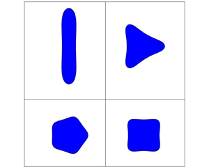
When a hollow vortex is steadily rotating an analytical treatment using free streamline theory is not straightforward since, on moving to a corotating frame, uniform vorticity is introduced. Nelson et al. (Reference Nelson, Krishnamurthy and Crowdy2020) instead devised a numerical method tailored to account for the doubly connected nature of the fluid exterior to the two vortices. As the angular velocity increases, each vortex is found to extend a thin finger towards the centre of rotation until the vortices almost touch; this sequence is shown from left to right in figure 1. Nelson et al. (Reference Nelson, Krishnamurthy and Crowdy2020) adapted their numerical scheme to compute the shape of a single 2-fold rotationally symmetric rotating hollow vortex. In that case, a thin waist forms in the vortex shape which eventually collapses; this sequence is shown from right to left in figure 1. Both sequences in figure 1 are found to approach the same limiting state. Nelson et al. (Reference Nelson, Krishnamurthy and Crowdy2020) argue this to be evidence of a topological singularity since the same state is approached from two topologically distinct directions but with no blow-up of any physical quantities.

Figure 1. Shapes of two steadily rotating hollow vortices, in the corotating frame, as computed numerically by Nelson et al. (Reference Nelson, Krishnamurthy and Crowdy2020). The present paper shows that the single rotating hollow vortices in the three right-most images can in fact be described in analytical form: they are the  $N=2$ case of a class of
  $N$-fold-symmetric ‘H-states’.
The purpose of this paper is to point out, first, that 2-fold rotationally symmetric solutions for a single hollow vortex computed numerically by Nelson et al. (Reference Nelson, Krishnamurthy and Crowdy2020) can, in fact, be written down analytically. It is then shown that this solution is just the  $N=2$ case of a family of solutions for
  $N$-fold rotationally symmetric rotating hollow vortices where
  $N \ge 2$ is an integer. Following Deem & Zabusky (Reference Deem and Zabusky1978), who used ‘V-states’ to refer to steadily rotating vortex patches, the analogous rotating hollow vortices derived here will be called ‘H-states’. For V-states, the
  $N=2$ solution is the celebrated rotating Kirchhoff ellipse which is a well-known exact solution of the two-dimensional Euler equations (Saffman Reference Saffman1992; Newton Reference Newton2001); none of the
  $N > 2$ V-states, however, can be written down in closed form and must be computed numerically (Deem & Zabusky Reference Deem and Zabusky1978). All H-state solutions, on the other hand, can be written down explicitly for any
  $N \ge 2$ as will be shown.
2. The H-state problem
The challenge is to find a single hollow vortex with unchanging shape, an ‘H-state’, with non-zero circulation  $\varGamma$ in steady solid body rotation with angular velocity
  $\varOmega$. The interior of the vortex is a constant pressure region. The flow
  $\boldsymbol {u} = (u,v)$ is incompressible so to describe the flow exterior to the vortex in a corotating frame we can introduce a streamfunction
  $\psi (x,y)$ such that
 \begin{equation} u = \frac{\partial \psi }{\partial y}, \quad v ={-} \frac{\partial \psi }{\partial x}. \end{equation}
Exterior to the vortex the streamfunction  $\psi$ satisfies
 \begin{equation} \nabla^2\psi ={-} \omega = 2\varOmega. \end{equation}
The kinematic condition that the vortex boundary is a streamline in the corotating frame, together with Bernoulli's theorem (Saffman Reference Saffman1992; Batchelor Reference Batchelor2000) and the condition that the pressure is continuous imply that, on the vortex boundary,
 \begin{equation} \boldsymbol{u} \boldsymbol{\cdot} \boldsymbol{n} =0, \quad \boldsymbol{u} \boldsymbol{\cdot} \boldsymbol{t} = q, \end{equation}
where  $\boldsymbol {n}$ is the outward normal to the vortex boundary and
  $\boldsymbol {t}$ is the tangent vector as the boundary is traversed in an anticlockwise direction. The constant
  $q$ is the fluid speed around the boundary. On introducing the complex variable
  $z=x+\textrm {i}y$ the two boundary conditions (2.3a,b) can be written in complex form as
 \begin{equation} u + \textrm{i} v = q \frac{\textrm{d}z }{\textrm{d}s}, \end{equation}
where  $\textrm {d}z/\textrm {d}s$ is the complex tangent and
  $\textrm {d}s$ is the arclength element that increases anticlockwise around the boundary. Equation (2.2) takes the form
 \begin{equation} \frac{\partial^2 \psi }{\partial z \partial \bar{z}} = \frac{\varOmega }{2} \end{equation}
which allows an integration with respect to  $z$ and
  $\bar {z}$
 \begin{equation} \psi =\frac{\varOmega }{2} z \bar{z} + \textrm{Im}[ w(z)], \end{equation}
where the analytic function  $w(z)$ is the complex potential for an irrotational flow component exterior to the vortex. From (2.1a,b) and (2.6) it can be deduced that
 \begin{equation} u - \textrm{i} v = 2 \textrm{i} \frac{\partial \psi }{\partial z} = \textrm{i} \varOmega \bar{z} + \frac{\textrm{d}w }{\textrm{d}z}. \end{equation}
It follows from (2.4) and (2.7) that, on the H-state boundary,
 \begin{equation} \textrm{i} \varOmega \bar{z} + \frac{\textrm{d}w }{\textrm{d}z} = q \frac{\textrm{d}\bar{z} }{\textrm{d}s}. \end{equation}
This boundary condition will determine both the H-state shape and the flow around it. The total circulation  $\varGamma$ of the H-state is
 \begin{equation} \varGamma = q \mathcal{P} + 2 \varOmega \mathcal{A}, \end{equation}
comprising a contribution from the constant tangential velocity  $q$ around the perimeter
  $\mathcal {P}$ and from the uniform vorticity
  $2 \varOmega$ over the H-state area
  $\mathcal {A}$. The relation (2.9) follows on integrating (2.8) with respect to
  $dz$ around the H-state boundary.
3. Exact solutions for H-states
It will be shown that the class of conformal mappings from the interior of the unit disc in a complex  $\zeta$-plane to the region exterior to an H-state in the corotating
  $z$-plane is
 \begin{equation} z= Z(\zeta) ={-}\frac{R }{\zeta} \left [ {1} + \frac{4 N }{(N-1)^2} \frac{\zeta^{N} }{\zeta^N-a^N} \right ], \quad 1 < a_{crit}^{(N)} < a, \quad N \ge 2, \end{equation}
where  $R > 0$ is a real normalization parameter that sets the size of the H-state. The limit
  $a \to \infty$ retrieves the circular hollow vortex of radius
  $R$. For each
  $N \ge 2$ there is a minimum critical value of
  $a$, denoted by
  $a_{crit}^{(N)}$, below which the shapes described by (3.1) are not univalent and are therefore not physically admissible; this loss of univalency is brought about by distinct parts of the vortex boundary coming into contact at
  $a=a_{crit}^{(N)}$ as will be seen later in figure 2. Actually, the class of conformal mappings (3.1) was first written down by Crowdy (Reference Crowdy1999a) for
  $N=2$, and for
  $N> 2$ (in a modified but equivalent form using the exterior of the unit disc as the preimage domain) by Wegmann & Crowdy (Reference Wegmann and Crowdy2000). The same mappings (3.1) are also used by Crowdy & Roenby (Reference Crowdy and Roenby2014). All this will be discussed in § 4. Crowdy (Reference Crowdy1999a) reports
  $a_{crit}^{(2)}=3.000$. The values
  $a_{crit}^{(3)}=1.690, a_{crit}^{(4)}=1.400, a_{crit}^{(5)}=1.277$ can be derived using the formula
  $a_{crit}^{(N)}=[(N-1)^{1/N} \tilde {a}_{crit}^{(N)}]^{-1}$ where
  $\tilde {a}_{crit}^{(N)}$ are the critical values of Wegmann & Crowdy (Reference Wegmann and Crowdy2000) who found numerically that
  $\tilde {a}_{crit}^{(3)}=0.4696, \tilde {a}_{crit}^{(4)}=0.5426$ and
  $\tilde {a}_{crit}^{(5)}=0.5934$. Formula (3.1) implies that on the H-state boundary, or
  $|\zeta |=1$,
 \begin{equation} \bar{Z}(\zeta^{{-}1}) ={-}{R \zeta} \left [ {1} + \frac{4 N }{(N-1)^2} \frac{1}{1- \zeta^N a^N} \right ], \end{equation}
where  $\bar {Z}(\zeta ) = \overline {Z(\bar {\zeta })}$ denotes the Schwarz conjugate function. It can also be verified, by direct differentiation, that
 \begin{equation} \left. \begin{gathered} \zeta Z'(\zeta) = \frac{ {R} }{(N-1)^2\zeta} \left [ \frac{(N+1)\zeta^N + (N-1)a^N }{(\zeta^N-a^N)} \right ]^2, \quad Z'(\zeta) \equiv \frac{\textrm{d}Z }{\textrm{d}\zeta},\\ \zeta^{{-}1} \bar{Z}'(\zeta^{{-}1}) = \frac{ {R} \zeta }{(N-1)^2} \left [ \frac{(N+1) + (N-1)\zeta^N a^N }{(1-\zeta^Na^N)} \right ]^2, \end{gathered} \right\} \end{equation}
and consequently that
 \begin{equation} \frac{\zeta^{{-}1} \bar{Z}'(\zeta^{{-}1}) }{\zeta Z'(\zeta)} = \zeta^2 \left [\frac{(N+1) + (N-1)\zeta^N a^N }{(1-\zeta^Na^N)} \times \frac{(\zeta^N-a^N) }{(N+1)\zeta^N + (N-1)a^N} \right ]^2. \end{equation}
Note from (3.3) the interesting features that  $\textrm {d}Z/\textrm {d}\zeta$ is a square of a rational function of
  $\zeta$, and has a rational function primitive. The boundary condition (2.8) valid on
  $|\zeta |=1$ implies that, on the H-state boundary,
 \begin{equation} \frac{\textrm{d}w }{\textrm{d}z} = q \frac{\textrm{d} \bar{z} }{\textrm{d}s} - \textrm{i} \varOmega \bar{z} =\textrm{i} {q} \left [ \frac{\zeta^{{-}1} \bar{Z}'(\zeta^{{-}1}) }{\zeta Z'(\zeta)} \right ]^{1/2} - \textrm{i} \varOmega \bar{Z}(1/\zeta), \end{equation}
where we have used the fact that  $\bar {\zeta } =1/\zeta$ on this boundary. On use of (3.2) and (3.4),
 \begin{align} \frac{\textrm{d}w}{\textrm{d}z} = \textrm{i}{q} \zeta \left [\frac{(N+1) + (N-1)\zeta^N a^N }{(1-\zeta^Na^N)} \times \frac{(\zeta^N-a^N) }{(N+1)\zeta^N + (N-1)a^N} \right ]\nonumber\\ +\,\textrm{i} \varOmega {R \zeta} \left [ {1} + \frac{4 N }{(N-1)^2} \frac{1}{1- \zeta^N a^N} \right ], \quad \textrm{on}\ |\zeta|=1, \end{align}
where we can think of the right-hand side as a function of  $z$ using the inverse function,
  $\zeta =Z^{-1}(z)$, of the conformal mapping (3.1). Both sides of (3.6) are analytic functions of
  $z$ that can be continued off the H-state boundary into the fluid domain exterior to it, or equivalently, inside the unit
  $\zeta$-disc. Remarkably, the right-hand side is a rational function of
  $\zeta$. Since we require
  $\textrm {d}w/\textrm {d}z$ to be free of singularities in the fluid region, and hence in
  $|\zeta | < 1$, it is necessary to remove the
  $N$ simple poles of the right-hand side of (3.6) at the roots of
  $\zeta ^N=1/a^N$ which are inside the unit
  $\zeta$-disc because
  $a > 1$. This can be done, by virtue of the
  $N$-fold rotational symmetry, by the single condition
 \begin{equation} q = \frac{2 \varOmega R }{(N-1)^2} \left [ \frac{(N-1)a^{2N} + N+1 }{a^{2N}-1} \right ] \end{equation}
obtained by setting the coefficient of  $(1-\zeta ^N a^N)^{-1}$ evaluated at
  $\zeta =1/a$ on the right-hand side of (3.6) equal to zero. Since, for the univalency of the mapping,
  $\textrm {d}Z/\textrm {d}\zeta$ must not vanish inside the unit disc, the right-hand side of (3.6) has no other singularities in this disc and therefore
  $\textrm {d}w/\textrm {d}z$ is analytic there, as required. Since as
  $\zeta \to 0$, or equivalently as
  $z \to \infty$, it follows from (3.6) and (3.1) that
 \begin{equation} \frac{\textrm{d}w }{\textrm{d}z} \sim{-} \frac{\textrm{i} R }{z} \left [{-}q \left ( \frac{N+1 }{N-1} \right ) + \varOmega R \left (1+ \frac{4N }{(N-1)^2} \right ) \right ], \end{equation}
and since it is required that
 \begin{equation} \frac{\textrm{d}w }{\textrm{d}z} \sim{-} \frac{\textrm{i} \varGamma }{2 {\rm \pi}z}, \quad \textrm{as}\ z \to \infty, \end{equation}
then a comparison of (3.8) and (3.9) shows it is necessary to pick parameters satisfying
 \begin{equation} \frac{\varGamma }{2 {\rm \pi}R } ={-}q \left ( \frac{N+1 }{N-1} \right ) + \varOmega R \left (1+ \frac{4N }{(N-1)^2} \right ). \end{equation}
Substitution of condition (3.7) into (3.10) produces
 \begin{equation} \varOmega = \left.\frac{\varGamma }{2 {\rm \pi}R^2} \right/ \left [ 1 + \frac{4N }{(N-1)^2} - \frac{2 (N+1) }{(N-1)^3} \left ( \frac{(N-1)a^{2N} + N + 1 }{a^{2N}-1} \right ) \right ], \end{equation}
which, for a given value of  $\varGamma$, is an explicit expression for the angular velocity
  $\varOmega$ in terms of the geometrical parameters
  $R, a$ and
  $N$. With
  $\varOmega$ thus determined, (3.7) gives
  $q$. With all parameters now known the velocity field follows, as an explicit function of
  $\zeta$, from (2.7) and the analytic continuation of (3.6) as
 \begin{align} u - \textrm{i} v = \textrm{i} \varOmega \overline{Z(\zeta)} &+ \textrm{i}{q} \zeta \left [\frac{(N+1) + (N-1)\zeta^N a^N }{(1-\zeta^Na^N)} \times \frac{(\zeta^N-a^N) }{(N+1)\zeta^N + (N-1)a^N} \right ]\nonumber\\ &\quad +\,\textrm{i} \varOmega {R \zeta} \left [ {1} + \frac{4 N }{(N-1)^2} \frac{1}{1- \zeta^N a^N} \right ]. \end{align}
The solution is complete and the H-states have been determined parametrically as explicit functions of  $\zeta$ for any
  $N \ge 2$. Conveniently, from the integral expressions
 \begin{equation} \mathcal{P} = \oint_{|\zeta|=1} \left| \frac{\textrm{d} Z }{\textrm{d}\zeta } \right| \frac{\textrm{d} \zeta }{\textrm{i} \zeta}, \quad \mathcal{A} ={-}\frac{1 }{2 \textrm{i}} \oint_{|\zeta|=1} \bar{Z}(\zeta^{{-}1}) \frac{\textrm{d}Z }{\textrm{d}\zeta}\,\textrm{d}\zeta \end{equation}
and use of residue calculus, it is easy to show that
 \begin{equation} \left. \begin{aligned} \mathcal{P} & = 2 {\rm \pi}R \left [\frac{2 N }{(N-1)^2} \left (\frac{(N-1)a^{2N} +N+1 }{a^{2N}-1} \right ) -\frac{N+1 }{N-1} \right ],\\ \mathcal{A} & = \frac{{\rm \pi} R^2 }{(1-a^{2N})^2 (N-1)^2} \left[ \left (\frac{N+1 }{N-1} \right )^2 (N^2-6N+1) \right.\\ & \left. \qquad - 2 \left (\frac{N+1 }{N-1} \right ) (N^2+4N-1) a^{2N} +a^{4N}(N-1)^2\right]. \end{aligned} \right\} \end{equation}
Such formulas are useful since, if one seeks H-states with fixed area  $\mathcal {A}={\rm \pi}$, say, then the second formula in (3.14) gives an explicit expression for
  $R$ in terms of
  $N$ and
  $a$. With parameters
  $q, \varOmega , \mathcal {P}$ and
  $\mathcal {A}$ determined by (3.7), (3.11) and (3.14), a consistency check on the solution is provided by confirming that (2.9) holds.

Figure 2. H-states for  $\mathcal {A}={\rm \pi}$ and (from left to right)
  $N=2,3,4$ and
  $5$. Parameter values are:
  $N=2, a=a_{crit}^{(2)}(=3.000), 3.5, 5, 10$;
  $N=3, a=a_{crit}^{(3)}(=1.690), 1.8, 2, 5$;
  $N=4, a=a_{crit}^{(4)}(=1.400), 1.5, 1.8, 5$;
  $N=5, a=a_{crit}^{(5)}(=1.277), 1.3, 1.5, 5$.
A purely numerical method to compute the H-state for  $N=2$ was given in Nelson et al. (Reference Nelson, Krishnamurthy and Crowdy2020) where the values of
  $q$ and
  $\varOmega$ associated with the critical state, corresponding to
  $a=a_{crit}^{(2)} = 3.000$, are reported for
  $\varGamma =2$ and
  $\mathcal {A} \approx 2 \times 0.311$. As a check on the above analysis, we can compute
  $q$ and
  $\varOmega$ using (3.7) and (3.11) with
  $\varGamma =2$, and
  $R$ calculated from the second formula in (3.14) with
  $\mathcal {A}={\rm \pi}$, to find
  $q \approx 0.236$ and
  $4 {\rm \pi}\varOmega \approx 1.347$ which coincide, to within numerical tolerance, with the (suitably rescaled) values reported by Nelson et al. (Reference Nelson, Krishnamurthy and Crowdy2020). A comparison of the shapes given by formula (3.1) for
  $N=2$ with those calculated numerically by Nelson et al. (Reference Nelson, Krishnamurthy and Crowdy2020) reveals them to be indistinguishable for arbitrary parameter values.
H-state shapes are shown for  $N=2,3,4$ and
  $5$ in figure 2. At
  $a=a_{crit}^{(N)}$ the H-states show an
  $N$-fold rotationally symmetric pinch-off where different parts of the boundary come into contact. These are quite different to the critical V-state shapes which are known to exhibit
  $90^{\circ }$ corner formation (Overman Reference Overman1986; Saffman Reference Saffman1992).
Figure 3 shows graphs of  $\varOmega$ and
  $q$ against
  $a$ for
  $N=2,3,4$ and
  $5$ for
  $\varGamma =1$ and
  $\mathcal {A}={\rm \pi}$. A bifurcation analysis from the circular state – that is, setting
  $Z(\zeta ) =-\zeta ^{-1} + \epsilon \zeta ^{N-1}$ in (3.5) and expanding for small
  $\epsilon \ll 1$ with
  $\varGamma =1$ – leads to
 \begin{equation} \varOmega \sim \frac{N-1 }{2 {\rm \pi}(N+1)}, \quad q \sim \frac{1 }{{\rm \pi}(N+1)}. \end{equation}
The curves in figure 3 tend to the values in (3.15a,b) as  $a \to \infty$ which corresponds to the near-circular state. As
  $a$ decreases from infinity
  $\varOmega$ and
  $q$ remain close to the values (3.15a,b) until
  $a$ gets close to
  $a_{crit}^{(N)}$ when they typically decrease monotonically (although a small increase in
  $q$ for
  $N=5$ is observed before it decreases).

Figure 3. Graphs of (a)  $\varOmega$ and (b)
  $q$ against
  $a$ for
  $N=2,3,4$ and
  $5$ and
  $\varGamma =1, \mathcal {A}={\rm \pi}$.
4. Perspectives
It is surprising that these exact solutions for such a basic class of distributed vortex structures have escaped notice for so long. This is likely due to the aforementioned observation that classical free streamline theory is unavailable as a route to their derivation. Like the Rankine vortex and the Kirchhoff ellipse, the results are valuable pedagogically in providing mathematically explicit desingularizations of an isolated point vortex.
The class of conformal mappings (3.1) was used first by Crowdy (Reference Crowdy1999a) and Wegmann & Crowdy (Reference Wegmann and Crowdy2000) to find solutions for a non-rotating hollow vortex but with the important difference that surface tension acts on its boundary. The boundary conditions are then more complicated because the fluid pressure is no longer constant on the vortex boundary but is balanced by a curvature-dependent surface tension term. As has been shown here, the class of shapes solving that quite different free boundary problem coincides with the H-state shapes. Indeed there is yet another distinct free boundary problem also solved by the same class of mappings (3.1): Crowdy & Roenby (Reference Crowdy and Roenby2014) found that they also solve the free boundary problem of a central hollow vortex, without surface tension, in equilibrium with an  $N$-polygonal array of satellite point vortices.
The work of Crowdy (Reference Crowdy1999a) and Wegmann & Crowdy (Reference Wegmann and Crowdy2000) emerged from insights gained from a new approach to free surface Euler flows with surface tension propounded by Crowdy (Reference Crowdy2000). There the author proposed a conformal mapping approach to understand why the classic problem of pure capillary waves on deep water studied by Crapper (Reference Crapper1957) admits exact solutions; he also sought to understand how Crapper's solution relates to analytical observations made by Tanveer (Reference Tanveer1996) on the functional form of conformal mappings to the region exterior to a translating bubble with surface tension, another example of a free surface Euler flow with surface tension. Crapper (Reference Crapper1957) used hodograph variables but it is not clear from his approach why his proposed solution ansatz works. Crowdy (Reference Crowdy2000) gained more insight by observing a Riccati-type structure to the analytically continued boundary condition that allowed deductions to be made on the functional form of the conformal mapping. He showed why Crapper's  $2 {\rm \pi}$-periodic solution must be given by the following log-rational mapping, from the unit
  $\eta$-disc, to a physical
  $\mathcal {Z}$ plane
 \begin{equation} \mathcal{Z} = \tilde{Z}(\eta) = {\textrm{i}} \left [ \log \eta - \frac{4 \hat{a} }{\eta-\hat{a}} \right], \quad \hat{a} > 1. \end{equation}
The arguments of Crowdy (Reference Crowdy2000) can be adapted to the present H-state problem to justify why the relevant conformal mappings must have the functional form (3.1).
In view of these analytical connections (Crowdy Reference Crowdy2000) between Crapper's capillary waves and hollow vortices with surface tension (Crowdy Reference Crowdy1999a; Wegmann & Crowdy Reference Wegmann and Crowdy2000), and since the same mappings (3.1) used in the latter problem also solve the H-state problem, it is natural to ask if the new H-state results in this ‘radial geometry’ might produce analogous exact solutions to some problem in Crapper's periodic water wave geometry. It turns out that such solutions have very recently been discovered by Hur & Wheeler (Reference Hur and Wheeler2020), whose work was motivated by a string of other recent contributions (Hur & Dyachenko Reference Hur and Dyachenko2019a, Reference Hur and Dyachenkob; Hur & Vanden-Broeck Reference Hur and Vanden-Broeck2020) where it was noticed that Crapper's capillary wave profiles were emerging in numerical simulations of rotational water waves. A similar thing happened here: noticing that the critical shape from Nelson et al. (Reference Nelson, Krishnamurthy and Crowdy2020) as shown in figure 1 is indistinguishable from the critical shape shown in figure 1 of Crowdy (Reference Crowdy1999a) led to the new H-state solutions. On making the identifications
 \begin{equation} \mathcal{Z} ={-} \textrm{i} \log z^N, \quad \eta = \zeta^N, \quad \hat{a} = a^N \end{equation}
with  $z$ related to
  $\zeta$ via (3.1) it can be shown that (4.1) is retrieved (to within unimportant additive constants) as
  $N \to \infty$. That is, the
  $N \to \infty$ limit of the H-states reproduces the water wave solutions of Hur & Wheeler (Reference Hur and Wheeler2020).
Actually, the surprising reappearance of Crapper's profiles in a problem different from the original problem of capillary water waves was noticed earlier by Crowdy & Roenby (Reference Crowdy and Roenby2014) who found exact solutions, given by Crapper's profiles (4.1), for steady water waves with vorticity: in their problem, the vorticity in each period window is concentrated in a submerged cotravelling point vortex. In view of the recent results of Hur & Wheeler (Reference Hur and Wheeler2020) the potential theoretic concept of ‘balayage’ (Shapiro Reference Shapiro1992) comes to mind: one imagines that the uniform vorticity in each period window in the Hur & Wheeler (Reference Hur and Wheeler2020) solutions is ‘swept’ into a single point vortex to give the solutions of Crowdy & Roenby (Reference Crowdy and Roenby2014) and without changing the wave profile.
It is intriguing that the same classes of mapping functions – the radial geometry shapes embodied in (3.1) and the Crapper-type periodic waves encoded in (4.1) – appear to be ‘canonical’ in that they recur in at least three physically distinct problems. As discussed by Crowdy & Roenby (Reference Crowdy and Roenby2014), this is likely due to the fact that (3.1) and (4.1) are the conformal mappings to so-called double quadrature domains which form an important class having their own mathematical significance; this is related to the features, noted in § 3, that  $\textrm {d}Z/\textrm {d}\zeta$ is both a square of a rational function of
  $\zeta$ and has a rational function primitive. A recent monograph (Crowdy Reference Crowdy2020) makes the case that the class of quadrature domains should be known more widely in the applied and physical sciences. They occur in various guises in fluid dynamics as surveyed by Crowdy (Reference Crowdy2005). We mention here that other classes of exact solutions – also viewable as quadrature domains – for steadily translating water waves with vorticity have been found by Crowdy & Nelson (Reference Crowdy and Nelson2010).
The results here point to the intriguing possibility that other analytical solutions exist for rotating hollow-vortex equilibria or those with background vorticity. In the corotating frame the H-states have a combination of uniform vorticity and concentrated boundary vorticity. They share these features with Sadovskii vortices (Saffman Reference Saffman1992) which have also received renewed attention (Freilich & Llewellyn Smith Reference Freilich and Llewellyn Smith2017). Zannetti et al. (Reference Zannetti, Ferlauto and Llewellyn Smith2016) computed the steady shapes of a hollow vortex in simple shear numerically, but it is conceivable that the analytical observations here are extendible to that problem which has many elements in common. Of course, whether the corotating hollow-vortex pair calculated numerically by Nelson et al. (Reference Nelson, Krishnamurthy and Crowdy2020) – i.e. the detached vortex pairs shown on the left in figure 1 – also admits analytical solutions is an open problem. In this regard it should be mentioned that, using the prime function for a concentric annulus (Crowdy Reference Crowdy2020), the author has extended the work of Crowdy (Reference Crowdy1999a) and Wegmann & Crowdy (Reference Wegmann and Crowdy2000) to find exact solutions for capillary waves on a fluid annulus with two free surfaces (Crowdy Reference Crowdy1999b, Reference Crowdy2001). Crowdy (Reference Crowdy1999b) also offered alternative forms, generalizing (4.1), of the capillary wave solutions on fluid sheets found by Kinnersley (Reference Kinnersley1977) who used Jacobi elliptic functions to generalize Crapper's solution. A similar approach using the prime function (Crowdy et al. Reference Crowdy, Llewellyn Smith and Freilich2013) also obviated the need for Jacobi elliptic functions in describing Pocklington's cotravelling hollow-vortex pair (Pocklington Reference Pocklington1895) and facilitated the calculation of its linear stability properties. The novel prime function approach to Kinnersley's solutions in Crowdy (Reference Crowdy1999b) might similarly uncover new solutions for water waves with vorticity on fluid sheets thereby generalizing the results of Hur & Wheeler (Reference Hur and Wheeler2020).
The stability of the H-states is clearly of interest, and can be studied using techniques similar to those used by Llewellyn Smith & Crowdy (Reference Llewellyn Smith and Crowdy2012) and Crowdy et al. (Reference Crowdy, Llewellyn Smith and Freilich2013). This matter remains to be investigated.
Funding
This research received no specific grant from any funding agency, commercial or not-for-profit sectors.
Declaration of interests
The authors report no conflict of interest.


