


1. Introduction
Ships and international trade are responsible for roughly $3$ % of global CO$_{2}$
 and Greenhouse Gas (GHG) emissions with an expected increase by $50$
 % to $250$
 % in the coming decades (Olmer et al., Reference Olmer, Comer, Biswajoy and Rutherford2017). Based on these findings, the International Maritime Organization (IMO) is developing a comprehensive strategy to reduce GHG emissions. This can be achieved in different ways: the optimisation of ship design; the development of new marine propulsion technologies; low-carbon and zero-carbon fuels; by improving the execution of ship operations; etc. As highlighted by Green et al. (Reference Green, Winebrake and Corbett2008), a proper operational planning and decision-making process can achieve a $2$
 %–$4$
%–$4$ % reduction on GHG emissions and environmental impact.
As a result, the field of operational planning has been the object of widespread research in the last decades covering different aspects. These range from weather forecasting, climate wave spectra (Boukhanovsky et al., Reference Boukhanovsky, Lopatoukhin and Soares Guedes2007; Degtyarev et al., Reference Degtyarev, Boukhanovsky, Lopatoukhin and Rozhkov2000) and safe ship navigation/handling to routing optimisation (Perera and Soares, Reference Perera and Soares2017 and references therein).
This paper presents a contribution to the field of operational planning by providing a novel methodology to support the decision-making process during the planning of vessel operations. More precisely, the proposed approach allows the post-analysis of the output generated by weather routing systems to assist the decision maker in identifying the most convenient Estimated Time of Departure (ETD)–Estimated Time of Arrival (ETA) window of opportunity to execute the desired operation.
The core of each ship route planning is represented by the weather routing system, which is designed for the estimation of the optimal route towards a selected destination as a function of the ship properties, travel distance/cost and the predicted METeorological and OCeanographic (METOC) state, to name a few.
The planning of the ship voyage can be formulated as a single-objective optimisation problem in which one criterion (e.g. voyage time) is optimised. Several methodologies have been developed for the computation of the optimal route. These range from the well-established isochrone method, proposed by James (Reference James1957), and its numerous improvements (Hagiwara and Spaans, Reference Hagiwara and Spaans1987; Lin et al., Reference Lin, Fang and Yeung2013) to dynamic programming (Zaccone et al., Reference Zaccone, Ottaviani, Figari and Altosole2018) or constrained graph problems, as in Mannarini et al. (Reference Mannarini, Pinardi, Coppini, Oddo and Iafrati2015) and Loeches et al. (Reference Loeches, Vicen-Bueno and Mentaschi2015) where the Dijkstra algorithm is used. In these, a graph of all the available routes between the departure and arrival locations is built, the edges of which are pruned where the defined constraints are not satisfied.
Given the particular nature of the problem being faced, the weather routing can be modelled considering the multi-objective optimisation perspective. This allows for the inclusion of multiple criteria in the process to compute the set of best routes in the Pareto sense. Multi-objective optimisation in the field of weather routing has seen increasing development together with the introduction of the evolutionary methodologies. This approach has been presented by Szlapczynska (Reference Szlapczynska2007), Marie and Courteille (Reference Marie and Courteille2009), Maki et al. (Reference Maki, Akimoto, Nagata, Kobayashi, Kobayashi, Shiotani, Ohsawa and Umeda2011), Fabbri et al. (Reference Fabbri, Vicen-Bueno, Grasso, Pallotta, Millefiori and Cazzanti2015), Vettor and Soares (Reference Vettor and Soares2016), Szlapczynska (Reference Szlapczynska2015) and references therein. All these exploit a genetic or evolutionary algorithm with multiple objectives in a continuos or discrete space to find the set of Pareto-optimal solutions. Each solution represents a different trade-off in terms of the selected conflicting objectives. At this stage, based on the computed routes, the decision maker selects the route representing the best trade-off among the available solutions. For a complete review on the mathematical approaches to weather routing systems, the authors refer to Walther et al. (Reference Walther, Rizvanolli, Wendebourg and Jahn2016).
The consequent post-analysis of the Pareto-set produced by a weather routing tool is not a straightforward process, especially for a human planner owing to the huge amounts of data to be analysed. Therefore a methodology to support the decision-making process is required. In Sidoti et al. (Reference Sidoti, Avvari, Mishra, Zhang, Nadella, Peak, Hansen and Pattipati2017), the authors propose the normalisation of the set of Pareto solutions after the algorithm termination. This allows a better comprehension of the impact of the conflicting metrics. This does not allow for the visualisation of other key variables characterising the decision-making process, such as the ETD and/or ETA. Chiu and Bloebaum (Reference Chiu and Bloebaum2009) proposed the Hyper Radial Visualisation (HRV) methodology, which enables an investigation of the trade-off decisions and the identification of better regions in a high-dimensional performance space. Szlapczynska (Reference Szlapczynska2007) and Li et al. (Reference Li, Wang and Wu2017) proposed the introduction of weighting coefficients plus a sorting methodology to identify the candidate route. Despite this, the above-mentioned papers and the references therein limit the decision-making process to the study of an ad hoc scenario with a predefined ETD for the selection of one route among those available to reach the destination.
As discussed by Perera and Soares (Reference Perera and Soares2017), an additional measure that can be incorporated into the weather routing and safe ship handling approaches is the exploitation of the information about the ETD and ETA. Estimated ETD–ETA values can be integrated into the port schedule to save on operating costs for both vessel and harbour operations (Kjetil, Reference Kjetil2004).
For the above-mentioned motivations, this paper presents a methodology to support the decision-making process during the planning of vessel operations. Starting from a selected kind of operation (e.g. travel/transit), this methodology has the goal of assessing, and consequently identifying, the best ETD–ETA window of opportunity to execute such an operation. Instead of summarising the computed routes through the view of the Pareto front (Szlapczynska, Reference Szlapczynska2015; Sidoti et al., Reference Sidoti, Avvari, Mishra, Zhang, Nadella, Peak, Hansen and Pattipati2017), the idea is to map the Pareto front into the ETD–ETA space through a metric expressing its operational safety (criterion based on the IMO safety guidelines IMO, 2007). As a result, a new way of visualising the huge amount of data produced by any weather routing tool is presented. This supports the decision maker in the selection of the optimal travel time window and produces an increased situational awareness. Furthermore, it allows the identification of new constraints to be enforced in terms of ETD or ETA for high-resolution route definition. The focus of this paper is therefore shifted from the formulation of the weather routing problem to the post processing of the data obtained from the solution of the optimisation problem. For this, a slightly different implementation (details provided in Section 2.3) of an existing weather routing system (developed by the authors in Fabbri et al., Reference Fabbri, Vicen-Bueno and Hunter2018; Fabbri and Vicen-Bueno, Reference Fabbri and Vicen-Bueno2019) is used for the computation of the optimal routes between two endpoints. The computed Pareto set (representing different trade-offs between conflicting metrics) is used as the input for the execution of the proposed decision-making methodology. In our previous works Fabbri et al., Reference Fabbri, Vicen-Bueno and Hunter2018; Fabbri and Vicen-Bueno, Reference Fabbri and Vicen-Bueno2019, we introduced the navigation risk metric as a safety measure to be optimised in the weather routing multi-objective set-up together with two other objectives (travel time and added resistance). In this work, we extrapolate this objective from the optimisation stage for its exploitation at the decision stage. This allows for the determination of the cumulative risk associated to each Pareto solution and the mean risk of each ETD–ETA window of opportunity. This enables an improvement of the computing performance owing to the reduced complexity of the optimisation problem and, at the same time, to include important information about the safeness of the routes at the decision stage. This represents an example on how an additional metric (e.g. risk metric) can be exploited for the ranking of the Pareto solutions in the ETD–ETA space.
The paper is organised as follows. The structure of the weather routing system is briefly recalled in Section 2. Section 3 presents the proposed decision-making methodology, which represents the main contribution of the paper. Section 4 presents the results of the approach tested in a real scenario for the determination of the best travel time window. Finally, a summary of the main findings is given in Section 5.
2. Ship operations decision-support system
In the context of ship operation planning, a standard Decision-support System (DSS) includes two main processing layers. First, the functionalities of weather routing for the generation of the set of routes, and second, the post-analysis of the routes to support the planner in making decisions in the easiest and most convenient way. These two processing layers are supported by two data layers, which define the environmental state and the ship properties. This is summarised in Figure 1, which shows the architecture of the considered DSS. Its main components are briefly detailed in the following subsections.
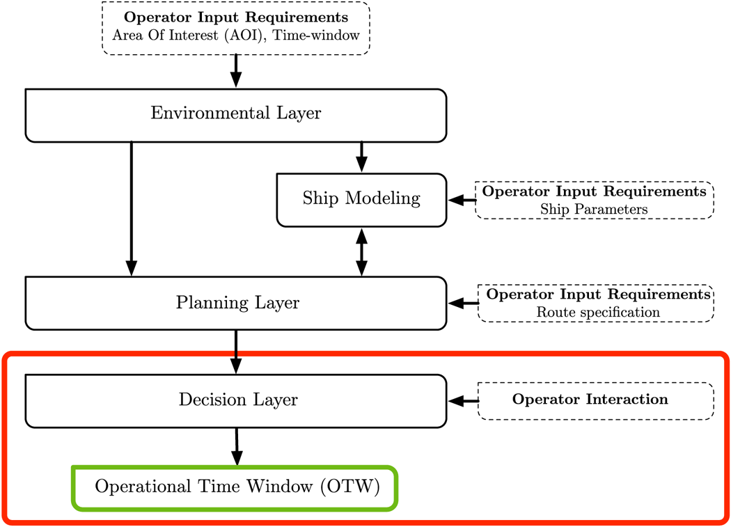
Figure 1. Common architecture of a ship operation decision-support system composed of $4$ main components: Environmental layer, Ship modelling, Planning layer and Decision layer. This paper is focused on the decision layer and the generated output Operational Time Window (OTW), which is highlighted in red
2.1 Environmental layer
The environmental layer retrieves and/or collects the set of METOC parameters needed to determine the evolution of the environmental state for the selected Area of Interest (AOI), both in time and space. The availability of weather forecast systems enables access to the predictions (short-term and long-term) of the required METOC variables.
To fully characterise the evolution of sea waves, the concept of climatic wave spectra has been recently developed (Degtyarev et al., Reference Degtyarev, Boukhanovsky, Lopatoukhin and Rozhkov2000; Boukhanovsky et al., Reference Boukhanovsky, Lopatoukhin and Soares Guedes2007; Neves et al., Reference Neves, Belenky, Kat, Spyrou and Umeda2011), which has resulted in the description of sea states as an ensemble of spectral models. However, this complete set of environmental data is not always available to the final user. As reported in the recent review by Žyczkowski et al. (Reference Žyczkowski, Szlapczynska and Szlapczynski2019), most of the operational weather forecast services do not provide the full spectra dependence (or ensemble forecasts) but only the long-term statistics of the state of the sea waves. For this reason, the considered implementation, described by Fabbri and Vicen-Bueno (Reference Fabbri and Vicen-Bueno2019), uses the average state of the sea waves for the selected AOI, but with increased resolution both in time and space, as the operational forecast service.
The selected parameters are those that have a direct impact on the motion and vulnerability of a selected ship. These are: significant wave height, $H_S$ (m); mean wave peak period, $T$
 (s); mean wave primary direction, $\alpha$
 ($^{\circ }$
 with respect to the North direction); mean wind direction, $\phi$
 ($^{\circ }$
 with respect to the North direction); and mean wind speed, $U_{10}$
 (m s$^{-1}$
 measured at $10$
 m above the sea-surface). The weather routing system also requires knowledge of the bathymetry or depth profile over the AOI to delimit the areas where the navigation is not allowed or difficult (e.g. identification of shallow water areas characterised by reduced manoeuverability (Vantorre et al., Reference Vantorre, Eloot, Delefortrie, Lataire, Candries and Verwilligen2017) or risk of grounding).
2.2 Ship modelling
The ship modelling is the component involved with estimating the dynamic behaviour of the vessel during navigation (wave and wind state provided by the environmental layer, Section 2.1). To model different ship types (e.g. cargo, container, tankers and military), a ship is defined through a synthetic set of parameters. These include:
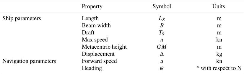
• the parameters defining the shape of the ship and its hull, such as: length; draft; beam width; metacentric height and displacement.
• the parameters defining the navigation state for the selected ship, such as the forward speed and heading associated with the route.
In our implementation, we consider the use of the semi-empirical ship operational model described by Lu et al. (Reference Lu, Turan, Boulougouris, Banks and Incecik2015). The selected methodology enables prediction of the added resistance experienced by the ship in different weather and sea conditions (irregular waves and wind). Consequently, we implemented this semi-empirical operational model (Lu et al., Reference Lu, Turan, Boulougouris, Banks and Incecik2015), owing to its limited computational cost. In addition, the well-known Holtrop and Mennen's Method (Holtrop and Mennen, Reference Holtrop and Mennen1982) is used for the estimation of the still-water resistance of the ship. The complete set of ship parameters considered in this model is listed in Table 1. The listed parameters enable an estimation of the sailing conditions and actual course of the selected ship based on the METOC conditions (from the environmental layer) in a given location within the AOI considering the ship's forward speed, $u$ , and heading, $\psi$
 . Because the purpose of this paper is focused on the identification of ETD–ETA windows of opportunity, the ship modelling component is defined with the goal and the advantage of being easily implemented and practical. For this reason, not all the aspects affecting the performance of the ship are modelled. Additional aspects, such as hull fouling, sea water temperature and sea currents (mean speed and direction), will cause additional speed losses for the ship.
Table 1. Ship and navigation parameters used in the ship modelling component
2.3 Planning layer
The planning layer represents the computational core of any weather routing system. The waypoints that compose the route are determined as a function of the METOC forecasts (provided by the environmental layer) and the vessel properties with the aim of optimising the selected cost(s).
The weather routing problem is addressed in our implementation as a multi-objective optimisation set-up and solved through the Martins labelling algorithm (Martins, Reference Martins1984). The selected algorithm is a generalisation of the Dijkstra shortest path algorithm (Dijkstra, Reference Dijkstra1959) to deal with a multi-objective set-up. Recalling the notion of the Pareto optimality: a route is Pareto optimal if and only if it is better than all the other routes for at least one objective and not worse than the other routes for the rest of the objectives. The selected algorithm computes the set of Pareto-optimal routes.
The domain of the available routes connecting the departure and arrival locations is defined in our implementation through a mathematical representation as a navigation graph (Fabbri and Vicen-Bueno, Reference Fabbri and Vicen-Bueno2019). Inspired by the isochrones method (Lin et al., Reference Lin, Fang and Yeung2013), each route is defined through the navigation graph by a set of consecutive location nodes (or waypoints) connected through linking edges (or seaways); each edge has associated with it a cost (in a single-objective set-up) or a set of costs (in a multi-objective set-up) that defines the price(s) to be paid to traverse it. It is worth mentioning that the costs associated with each edge change with the time and space owing to the variability of the METOC conditions over the AOI in the considered temporal window. The Martins algorithm determines the complete set of Pareto-optimal routes. Each route is represented by an ordered sequence of nodes and edges with an associated optimal (in the Pareto sense) cumulative cost (as the sum of the costs associated with the edges composing the route) between the departure and destination locations. The multi-objective optimisation is defined by two conflicting criteria to be minimised:
Cost 1 - Travel time
The travel time represents an estimate of the time required to traverse the selected edge between two node locations. This is computed as a function of the actual sailing conditions by taking into account the average METOC conditions for the selected time interval. The implemented approach (Loeches et al., Reference Loeches, Vicen-Bueno and Mentaschi2015) assumes the ship moves between two consecutive node locations (waypoints) at a constant speed.
Cost 2 - Added resistance
The added resistance criterion models the forward speed reduction of the ship arising from the added resistance from weather conditions (sea waves and wind) when considering a selected course. The added resistance follows the empirical approach defined by Lu et al. (Reference Lu, Turan, Boulougouris, Banks and Incecik2015). This criterion enables an estimation of the resistance caused by the waves and the average percentage of speed loss, compared with the speed in still-water conditions, experienced by the ship when traversing the selected edge in a given time step. The selected criteria are aligned with the mission objectives of identifying the routes that minimise both the travel time to reach the desired destination (from Cost 1) and the mitigation of the METOC effects as much as possible. Considering this implementation, the minimisation of the added resistance has been selected as an optimisation criterion because it allows a measure of how far the ship is from the navigation in still-water conditions. This allows us to keep the implementation as general as possible without considering additional information about the selected ship (e.g. the efficiency of transmitted power). Because the process of computing the set of Pareto-optimal routes for a weather routing scenario (e.g. departure and destination locations, AOI time frame) is beyond the scope of this paper, we recall the reference papers of Fabbri and Vicen-Bueno (Reference Fabbri and Vicen-Bueno2019) and Fabbri et al. (Reference Fabbri, Vicen-Bueno and Hunter2018) for the implementation details.
3. Decision layer: Operational time window (OTW)
The decision layer represents the architectural component characterised by a strong interaction with the decision maker. As discussed in the previous sections, the decision layer is not limited to the selection of the route representing the best trade-off (in this implementation, the minimisation of travel time and added resistance) among the computed routes. Usually, two stages of planning are executed (Sidoti et al., Reference Sidoti, Avvari, Mishra, Zhang, Nadella, Peak, Hansen and Pattipati2017):
• The first stage provides the so-called movement report at least $72$
 h before embarkation, which indicates the departure time, intended arrival time and other data;
• The second stage provides the recommended route $36$
h prior to departure.


Unexpected inconveniences may not allow the predefined plan to be followed: a delay of a few hours in the departure time may require the execution of a new weather routing process, owing to the varying METOC conditions in the AOI. As a consequence, a revised plan may generate routes that were determined by different decisions. This represents an example of the possible limitations that the current decision layer suffers as a result of unexpected inconveniences. For the above-mentioned considerations, new methodologies are required to support the decision-making process to take into account inconveniences that may be encountered.
3.1 Prior steps to OTW estimation
The approach we propose is to identify the OTW during the decisional stage as a post-analysis of the set of Pareto-optimal routes.
Usually, given a selected ship, a weather routing process is characterised by:
• Departure and destination locations.
• Temporal constraints in which the journey has to be executed in terms of ETD and ETA.
For a given scenario, the OTW enables the determination of the recommended temporal window (in terms of ETD–ETA) to perform the transit or a predefined operation between the departure and destination locations. More precisely, the OTW determines the range of contiguous ETD and ETA values, which is characterised by high operational safety, considering the METOC state faced by the selected ship. To this end, the set of Pareto-optimal routes are ranked based on its temporal information: the ETD set during the weather routing setup by the user and the resulting ETA. This is easily achieved through a temporal two-dimensional (2-D) grid, in which the $x$ and $y$
 axes are associated to different temporal ranges of ETD and ETA, respectively. Figure 2 shows an example of a temporal grid characterised by a temporal resolution of $1$
 h in both axes. Each $1\,\textrm {h}\times 1\,\textrm {h}$
 cell or bin contains all the Pareto-optimal routes produced by the weather routing process (depicted as blue markers), which are characterised by the ETDs and ETAs values falling within the considered bin.
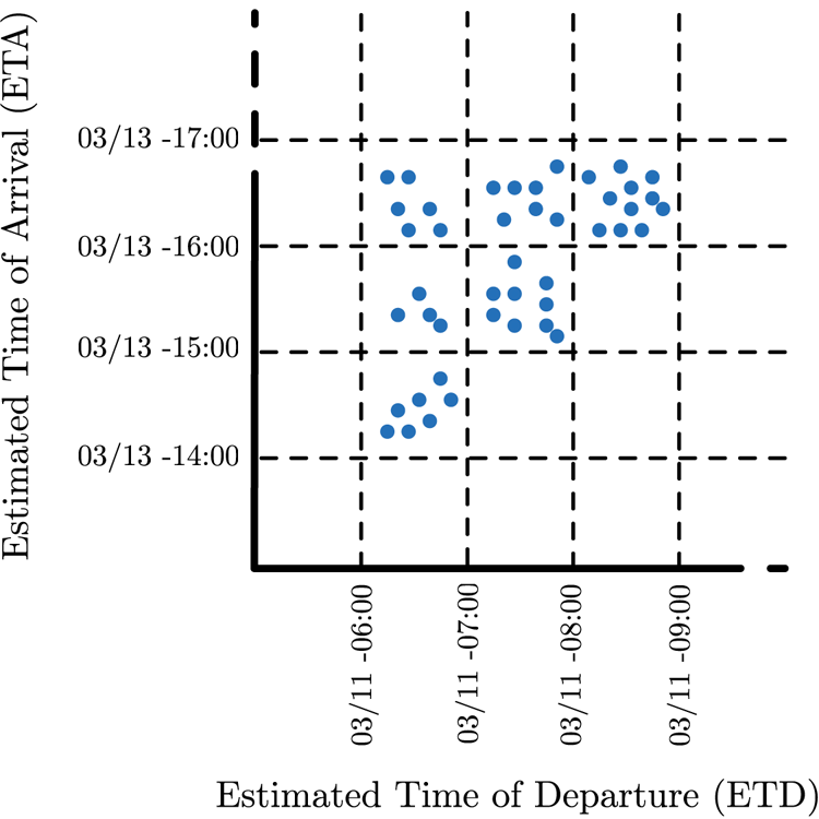
Figure 2. Temporal grid associated with the set of Pareto-optimal routes computed by the planning layer. Each $1\,\textrm {h}\times 1 \,\textrm {h}$ cell collects the Pareto-optimal routes characterised by common timing properties (ETD and ETA bin)
For a given scenario, this representation allows: first, to group together the routes based on common timing constraints; and, second, the estimation of the limits in terms of travel time for different ETDs, which have different METOC conditions in the AOI.
It is worth mentioning that the temporal grid presented in Figure 2 is the result of the execution of the same weather routing process but varying the ETD within the temporal range considered.
The idea we pursued is to characterise the representation of Figure 2 with additional information/data that would be helpful at this stage for the decision maker for the determination of the OTW. Starting from the temporal grid representation (Figure 2), our goal is to determine the range of ETD–ETA bins, and the Pareto-optimal routes therein, which represent the most convenient choices to perform the selected transit/operation. To this aim, our approach characterises each Pareto-optimal route with an additional measure that represents its operational safety. This is inspired by the IMO guidelines for the ship masters to avoid dangerous situations in adverse weather conditions (IMO, 2007). The details regarding the computation of the OTW are reported in Section 3.2.
3.2 OTW procedure
Starting from the set of Pareto-optimal solutions (computed by the planning layer), the OTW is computed. The procedure is characterised by $4$ steps, as depicted in Figure 3. The first $3$
 steps show the process of estimating the operational safety, $O(r)$
 , starting from an input Pareto-optimal route $r$
 . These $3$
 steps are repeated for each Pareto-optimal route computed by the planning layer. Finally, the fourth step computes the OTW representation, which considers all the Pareto-optimal routes. The detailed description is reported below.
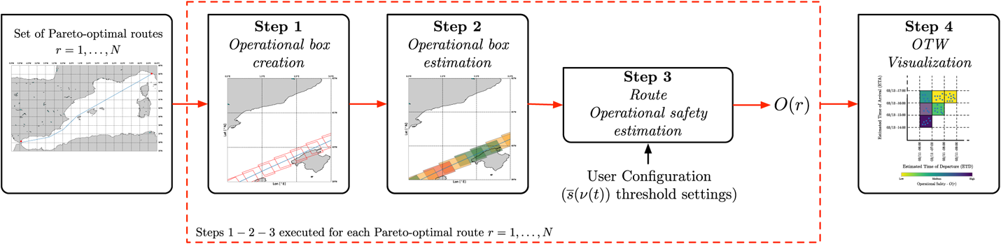
Figure 3. Steps executed for the determination of the OTW representation associated with the set of Pareto-optimal routes provided by the planning layer
3.2.1 Step 1: Operational boxes creation
A set of overlapping operational boxes is determined along the route. The dimensions of each operational box reflect the operational requirements defined by the decision maker. For example, the length (along the route) can be equal to the distance covered by the ship travelling at a constant cruise speed for a predefined number of hours (e.g. for a cruise speed $=$ 20 kn for 2 h, the length of the rectangular area is $\approx$
 40 nmi).
The width of the operational box is set by the decision maker as an input based on specific operational requirements, e.g. size of the area to be surveyed and to model the ship deviations that may occur from the selected route. The operational boxes are placed along the selected route ensuring that each operational box overlaps with the one that follows. The maximum portion of overlapping area is set by the decision maker as an input to the system. The maximum overlapping area occurs when two consecutive operational boxes are aligned.
3.2.2 Step 2: Operational box estimation
Starting from the set of boxes (from Step 1) associated with the route $r$ , this step quantifies the average safety distance between the safe sailing conditions and the estimated navigation conditions faced by the selected ship when sailing within each box for the considered time step. This measure is a function of the METOC conditions at the time of passing through it, as well as the ship parameters (see Table 1).
The safety distance is derived from the guidelines provided to navigators for adverse weather conditions (IMO, 2007; Fabbri and Vicen-Bueno, Reference Fabbri and Vicen-Bueno2019). The dangerous situations considered in this work are: surf-riding and broaching-to; successive high-wave attack; synchronous rolling; and reduction of intact-stability when riding on a wave crest.
Recalling the methodology of Krata and Szlapczynska (Reference Krata and Szlapczynska2012) and Przemyslaw and Joanna (Reference Przemyslaw and Joanna2018), the IMO dangerous areas can be depicted in a polar plot, as highlighted by the red, green and blue areas in Figure 4. Each point $p$ within the polar plane is defined by its angle (taken in the clockwise direction with respect to the upward direction) and radial distance from the centre, which represent the wave encounter angle and the forward speed (in kn) of the ship, respectively. Here, $p$
 is defined as all possible configurations of the ship.
Figure 4. Representation of the dangerous areas according to the guidelines of (IMO, 2007) over a polar plane (angle and distance from the centre represent the wave encounter angle and the forward speed of the ship, respectively): surf-riding and broaching-to in blue, resonance in red and successive high-wave attack in green
From this representation, the safety distance, $s(\nu (t))$ , is defined as the normalised distance between the actual ship configuration, $\nu (t)=[u(t), \psi (t)]$
 , (blue marker in Figure 4) and the closest IMO dangerous area, as summarised in Equation (1).

where $p \in \mathcal {D}_{\textrm {IMO}}(t)$ represents the subset of ship configurations within the IMO dangerous areas (red, green, blue areas in Figure 4). The dangerous areas are determined based on the actual METOC conditions at the selected time step $t$
 and ship parameters (IMO, 2007). Here, $\nu (t)$
 is the vector representing the current ship configuration (forward speed $u(t)$
 and the derived wave encounter angle from the selected heading $\psi (t)$
 ) in the polar plane. The absolute distance between two points in the polar plane is $\|\cdot \|$
 . The range of the radial axis in the same polar plane (or norm of the difference between the two 2-D vectors) is $r_{\max }$
 . This quantity is represented by the magnitude of the maximum forward speed of the ship, $\overline {u}$
 . The safety distance, $s(\nu (t))$
 , has values in the range $[0,1]$
 , where the two range ends, $0$
 or $1$
 , represent that the ship is operating in dangerous or safe conditions, respectively. In the case where the ship configuration $\nu (t)$
 falls within the $\mathcal {D}_{\textrm {IMO}}(t)$
 , the safety distance $s(\nu (t))$
 is $0$
 , which represents a dangerous situation for the ship. To characterise each operational box, the computation of $s(\nu (t))$
 is repeated for all the locations within the operational box under analysis to determine the mean safety distance measure, $\overline {s}(\nu (t))$
 , associated with each box. The number of locations and the locations to be investigated are directly determined by the spatial resolution of the METOC forecasts provided by the environmental layer. It is worth pointing out that $\overline {s}(\nu (t))$
 is directly related to the METOC conditions faced by the ship at the time step $t$
 considering the ship configuration $\nu (t)$
 (forward speed and wave encounter angle) associated with the transect of the Pareto-optimal route falling within the investigated operational box. Finally, to analyse the information associated with each Pareto-optimal route and give an understandable representation of the route to the operator, $3$
 levels of $\overline {s}(\nu (t))$
 are defined (with the associated colours).
• $0{\cdot }65 < \overline {s}(\nu (t)) \le 1$
- High safety distance - Violet.• $0{\cdot }35 < \overline {s}(\nu (t)) \le 0{\cdot }65$
- Medium safety distance - Blue.• $0 < \overline {s}(\nu (t)) \le 0{\cdot }35$
- Low safety distance - Yellow.


3.2.3 Step 3: Route operational safety - $O(r)$

This step determines the cumulative operational safety associated with the route under analysis. More precisely, this stage is based on a set of logic rules derived from navigator knowledge and experience. As a matter of fact, the determination of the cumulative operational safety as a direct average of the $\overline {s}(\nu (t))$ value associated with each box along the route leads to a result that may underestimate $O(r)$
 . For example, few boxes with a low value of $\overline {s}(\nu (t))$
 are filtered out by the remaining boxes with a high value of $\overline {s}(\nu (t))$
 , which results in a route that is convenient for transit even in the case where the section with the boxes with low safety makes the route not viable. For the above-mentioned motivations, the cumulative $O(r)$
 associated with each route is based on the definition of a set of rules able to identify the maximum portion of the travel time, so the ship and therefore its crew are characterised by reduced operational safety. The set of rules are specified in Table 2. This table also reports the set of thresholds identifying the five levels of operational safety. The fuzzy rules for the determination of the cumulative operational safety includes degrees of freedom (including change of thresholds). This allows the decision maker/navigator to interact with the system based on their experience. The thresholds provided in Table 2 are defined from actual experience at CMRE. These thresholds could be changed during the decision-making process as a consequence of the operator requirements. This allows the navigator/decision maker to configure the system based on the mission/operation (e.g. transport of sensitive material). It is worth mentioning that the definition of these thresholds requires a careful validation during extensive tests in future research before real-life applications. This step also allows the decision maker to gain the required experience with the proposed methodology to obtain the appropriate results based on the capabilities of the selected ship. It is worth pointing out that the routes characterised by at least a ship configuration $\nu (t)$
 that leads to a safety distance $s(\nu (t)) = 0$
 are tagged as low-operational safety, without considering the set of rules previously defined (Table 2).
Table 2. Fuzzy rules determining the operational safety, $O(r)$ , associated with a given route ($r$
 ) through the percentage of boxes within a mean safety distance, $\overline {s}(\nu (t))$
 , level
3.2.4 Step 4: OTW visualisation
Finally, the $O(r)$ of each Pareto-optimal route is exploited to add new information to the previous representation of Figure 2. This is done by associating each ETD–ETA cell with the mean value of $O(r)$
 of the Pareto-optimal routes falling in it. The colour code associated with each cell is defined by the average cumulative $O(r)$
 of the routes characterised by the same ETD–ETA cell. An example is shown in Figure 5 using a colour map to represent the mean operational safety associated with each ETD–ETA cell. The colours violet, blue and yellow represent high, medium and low mean $O(r)$
 , respectively, as depicted in the colour bar of Figure 5.
Figure 5. Example of OTW representation of the Pareto-optimal routes produced by the planning layer for a given time frame. The colour associated with each cell represents the mean value of the operational safety metric, $O(r)$ , of the routes with ETD and ETA values within a $1\,\textrm {h}\times 1\,\textrm {h}$
 cell
cell
The OTW representation is exploited as a decision-making tool to visually identify the intervals of ETD and ETA characterised by high (green) and low (red) mean $O(r)$ . As a consequence, the routes within that temporal interval are characterised by favourable and or unfavourable sailing conditions for the execution of the selected operation. From this result, the decision maker can execute the weather routing process (planning layer) at higher resolution in a more constrained time-window to generate the final plan for the ship. The proposed approach is tested for a concrete use case in Section 4.
4. Scenario and results
4.1 Scenario set-up
The proposed methodology is tested for the scenario of planning the transit in the Mediterranean Sea between the ports of La Spezia (ITA) and Gibraltar (UK). The limits of the AOI and the selected temporal window are:
• Longitude range: from $6{\cdot }5^{\circ }$
W to $10{\cdot }5^{\circ }$E.• Latitude range: from $35^{\circ }$
to $45^{\circ }$N.• Temporal window: ETD in the interval between June 14th, 2018, at 15:00 UTC and June 15th, 2018, at 07:00 UTC.


4.2 Nominal route and analysis of a Pareto-optimal route
Figure 6 shows the nominal route between La Spezia (ITA) and Gibraltar (UK) provided by the web-service searoutes.com (Maritime Data Systems, 2018). It also shows the location nodes (or waypoints) that compose the domain of alternative seaways between the departure and destination ports. The nominal route represents the shortest suggested route to reach the desired destination. The selected AOI and time frame represent a good test case for evaluating the proposed approach owing to the presence of a storm crossing the AOI, as depicted in Figure 7. It shows $6$ snapshots of $H_S$
 taken every $10$
 h in the time window under study. As observed in Figure 7(a,c), the storm is characterised by waves of $H_S \approx 6$
 m in the north-west area of the AOI. These environmental conditions affect the planning of operations as discussed below.
Figure 6. Nominal route (blue) between La Spezia (ITA) and Gibraltar (UK) ports (Maritime Data Systems, 2018). The black markers around the nominal route are the location nodes that compose the navigation graph, which indicate the domain of available routes between the two ports
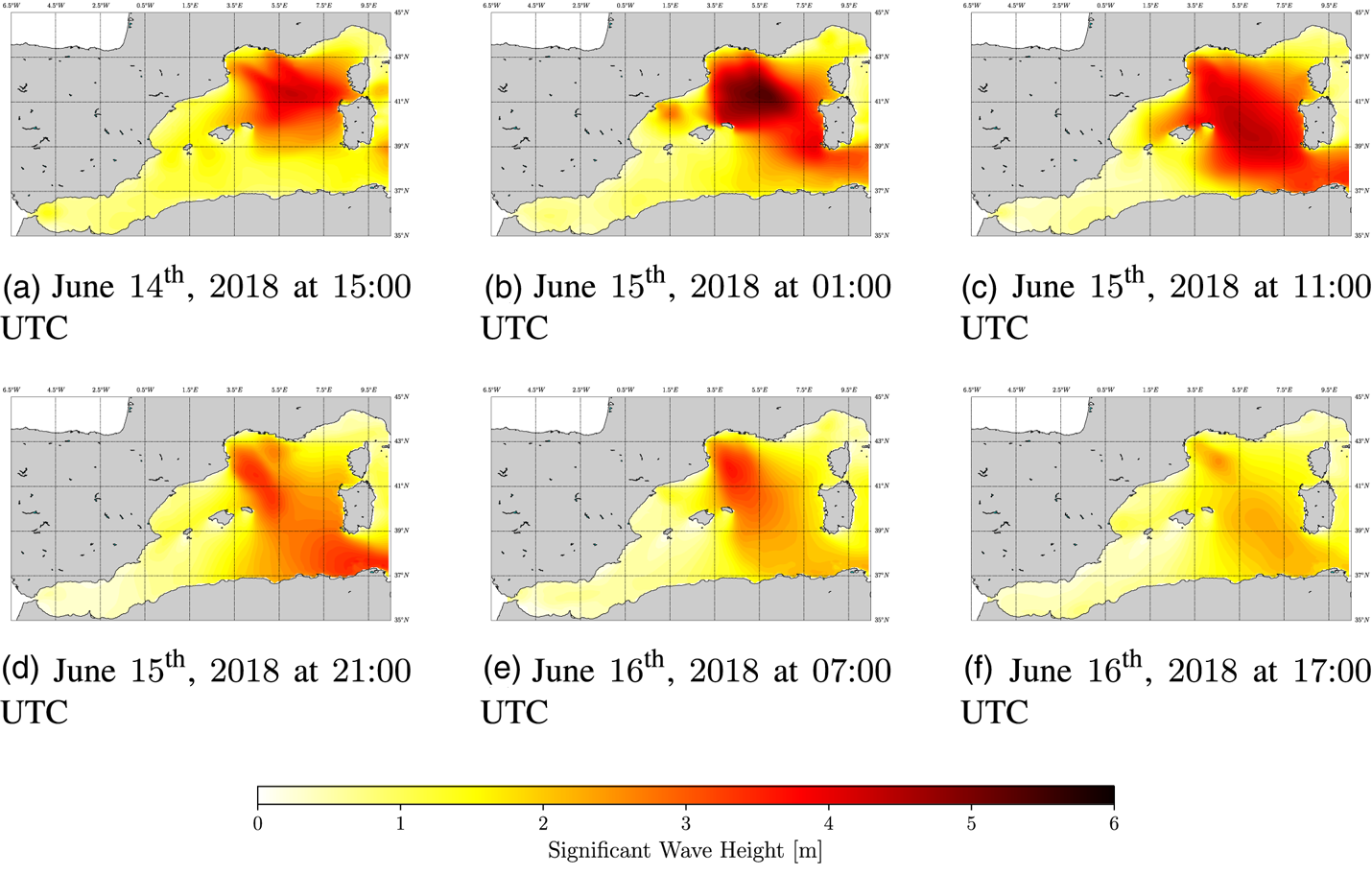
Figure 7. Evolution of the significant wave height, $H_S$ , in the AOI and temporal window [June 14th, 2018, at 15:00 UTC–June 15th, 2018, at 07:00 UTC]. Snapshots taken every $10$
 h. (a) June 14th, 2018 at 15:00 UTC, (b) June 15th, 2018 at 01:00 UTC, (c) June 15th, 2018 at 11:00 UTC, (d) June 15th, 2018 at 21:00 UTC, (e) June 16th, 2018 at 07:00 UTC, (f) June 16th, 2018 at 17:00 UTC
In the set-up taken for our experiment, the environmental layer (Figure 1) provides the METOC data for the selected AOI in the form of a gridded forecast (Mentaschi et al., Reference Mentaschi, Besio, Cassola and Mazzino2013) provided by DICCA-MeteOcean (Dipartimento di Ingegneria Civile, 2018). The provider based its forecasting service on the Wavewatch III model (National Weather Service - Environmental Modeling Center, 2018). The forecasts are characterised by a spatial-temporal grid with a $10$ km ($5{\cdot }31$
 nmi) spatial resolution in both latitude and longitude and a time resolution of $1$
 h over the whole Mediterranean basin. The provided data covers a temporal window of $120$
 h, starting at 00:00 UTC, with new forecasts generated everyday. The uncertainty associated with the METOC variables is not available. The environmental data also include the bathymetry/depth profiles (EMODnet Bathymetry - The European Marine Observation And Data Network, 2018) that cover the whole AOI, with a spatial resolution of $115$
 m in both longitudinal and latitudinal directions. The bathymetric profiles are used to identify the shallow water areas characterised by reduced manoeuverability (Vantorre et al., Reference Vantorre, Eloot, Delefortrie, Lataire, Candries and Verwilligen2017). The scenario considers a typical multi-role patrol frigate with the properties defined in Table 3.
Table 3. Ship parameters used in the weather routing scenario
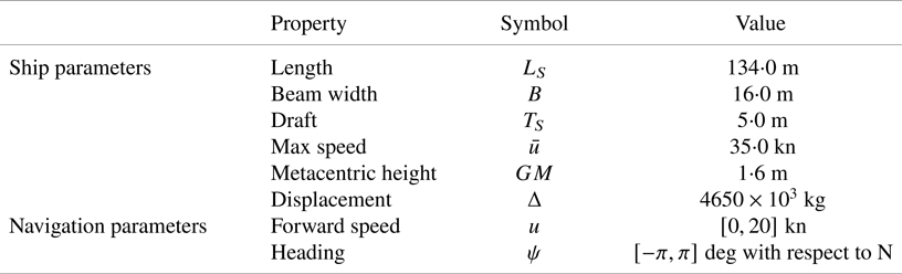
In a typical set-up, a weather routing process considers a predefined ETD for the determination of the set of Pareto-optimal routes (considering a multi-objective optimisation configuration). Considering ETD as June 14th, 2018 at 20:00 UTC, Figure 8(a) presents the set of Pareto-optimal routes obtained by our proposed implementation. They are computed by the planning layer using the minimisation of both the travel time and added resistance as conflicting costs. Following the classical approach, the decision layer has to select the candidate route based on predefined procedures (e.g.: HRV, ranking methods, etc). In our case, instead of following the classical approach, our goal is to identify the temporal intervals in terms of ETD–ETA presenting the best conditions to execute the transit between the departure and destination locations. For this reason, the analysis of the identification of the candidate route for a selected ETD is beyond our scope and so is not presented in this paper. In our implementation, the decision layer executes the OTW procedure (see Section 3 and Figure 3). From each Pareto-optimal route, $r$ , the operational safety, $O(r)$
 , is computed. Figure 8(b) shows the output of step $2$
 of Figure 3 (operational box estimation) for a given route of the set of Pareto-optimal routes. In our scenario, each operational box along the route is $74$
 km long and $35$
 km wide. The length of the operational box is determined by the distance covered by the ship at its maximum cruise speed (20 kn) for a period of $2$
 h. The operational box width is set as a configuration parameter by the decision maker and it is used to model the ship deviations that may occur from the selected route. As shown in Figure 8(b), the first half of the selected route is approximately characterised by a medium (blue)-to-low (yellow) mean safety distance. This arises from the adverse METOC conditions and dangerous navigation conditions that the ship may face during the transit (Figure 7). The second half of the route is characterised instead by a high safety distance (violet) owing to more favourable METOC conditions. Finally, $O(r)$
 is computed: the selected Pareto-optimal route is characterised overall by a medium-low operational safety owing to the long exposure of the ship to low safety distance conditions (blue, yellow operational boxes).
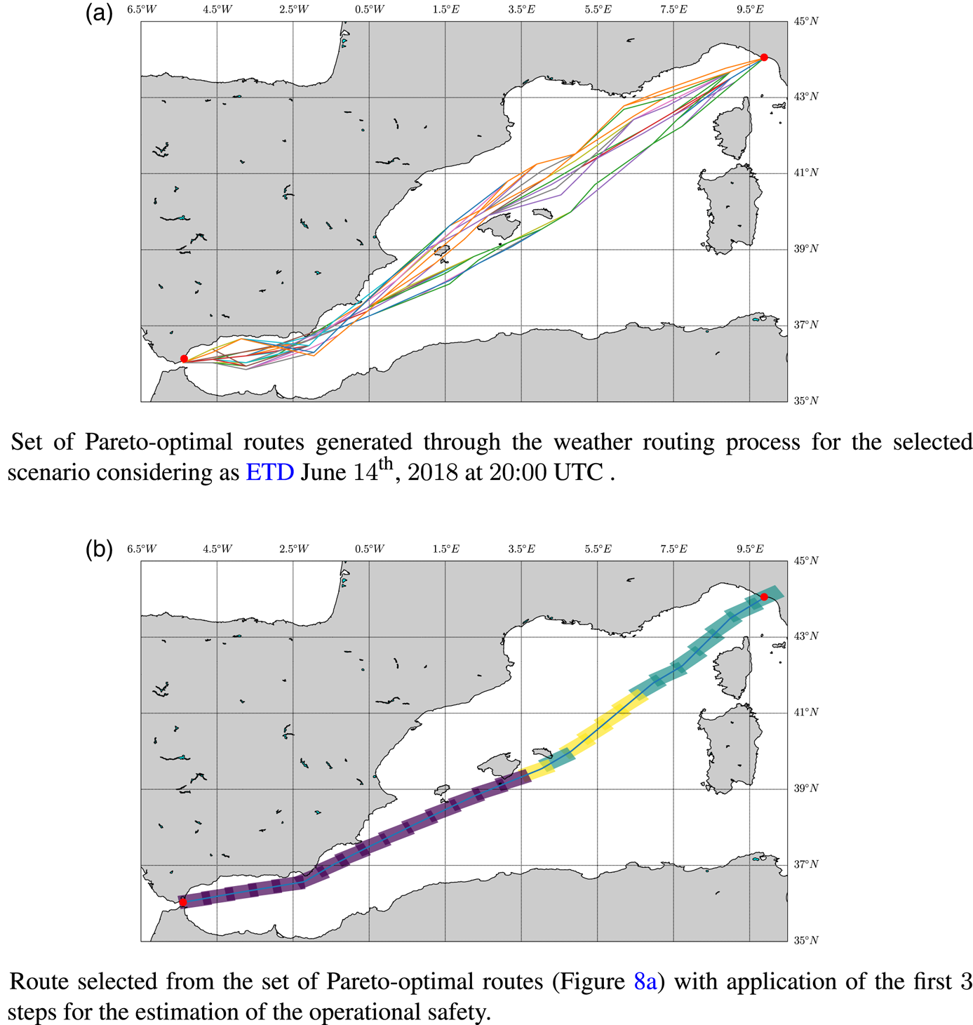
Figure 8. Example of the analysis by the proposed weather routing system for the selected AOI and given ETD: (a) shows the output generated at the planning layer; (b) presents the post analysis of a Pareto-optimal route for estimating its operational safety. (a) Set of Pareto-optimal routes generated through the weather routing process for the selected scenario considering ETD as June 14th, 2018 at 20:00 UTC. (b) Route selected from the set of Pareto-optimal routes in (a) with application of the first $3$ steps for the estimation of the operational safety
4.3 Analysis of the full set of Pareto-optimal routes for different ETDs (ETD interval)
The analysis described above has been applied to a single Pareto-optimal route within the set of routes computed for a single ETD. In our approach, the weather routing process is repeated for each ETD within the selected temporal window of $16$ h (from June 14th, 2018 at 15:00 UTC to June 15th, 2018 at 07:00 UTC). This process produces a set of $932$
 Pareto-optimal routes as depicted in the temporal grid of Figure 9(a), where each $1\,\textrm {h} \times 1\,\textrm {h}$
 cell collects the Pareto-optimal routes within $1\,\textrm {h} \times 1\,\textrm {h}$
 ETD–ETA intervals. Each Pareto-optimal route is analysed following the procedure applied previously to the route depicted in Figure 8(b). The application of this procedure (Figure 3) allows an association of each ETD–ETA cell with the mean value of the operational safety. Considering the whole temporal grid, the OTW is depicted in Figure 9(b).
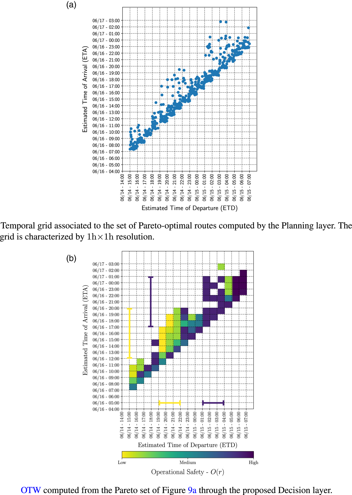
Figure 9. Analysis of the set of Pareto-optimal routes provided by the planning layer for a temporal window of $16$ h: (a) shows the Pareto-optimal routes in a temporal grid with $1\,\textrm {h} \times 1\,\textrm {h}$
 resolution; (b) shows the OTW representation through the proposed decision layer. (a) Temporal grid associated to the set of Pareto-optimal routes computed by the planning layer. The grid is characterised by a $1\,\textrm {h} \times 1\,\textrm {h}$
 resolution. (b) The OTW computed from the Pareto set in (a) through the proposed decision layer
From the analysis of the OTW representation, the decision maker can easily identify temporal windows of opportunity in which the execution of the transit is suggested or not. Analysing the results in Figure 9 show:
• Low operational safety interval: the Pareto-optimal routes with ETD in the interval June 14th, 2018, [19:00–22:00] UTC and ETA in the interval June 16th, 2018, [12:00–20:00] UTC are identified with low (red) mean operation safety. This arises from the adverse METOC conditions that the ship may face considering the routes within such an ETD–ETA window. This fact is highlighted in Figure 7(a–c), where $H_S$
reaches up to $6$ m. This is also highlighted in the analysis of the single route depicted in Figure 8(b), where the first portion of the route is characterised by a medium-low operational safety.• High operational safety interval: the routes in the temporal window with ETD in the interval June 15th, 2018, [01:00–04:00] UTC and ETA in the interval [June 16th, 2018, 17:00 UTC, June 17th, 2018, 01:00 UTC] are characterised by a high mean operational safety. This is motivated by the ending of the METOC perturbation crossing the AOI, as shown in Figure 7(d–f).


4.4 Assessment and analysis of OTW
A deeper analysis of why these two ETD time intervals are sorted as low and high operational safety, respectively, is provided below. To this aim, the METOC conditions associated with the Pareto-optimal routes within the low operational safety cells (red colour) (ETD in the interval June 14th, 2018, [19:00–22:00] UTC and ETA in the interval June 16th, 2018, [12:00–20:00] UTC) are compared with the METOC conditions of the Pareto-optimal routes within the high operational safety cells (ETD in the interval June 15th, 2018, [01:00–04:00] UTC with ETA in the interval [June 16th, 2018, 17:00 UTC, June 17th, 2018, 01:00 UTC]). These are depicted in Figures 10–12.
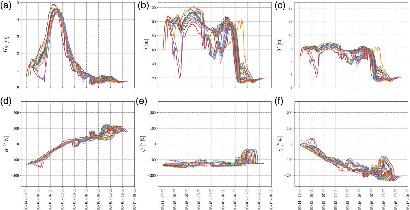
Figure 10. Low operational safety OTW–METOC conditions characterising the routes with low operational safety in the temporal window with ETD in the interval June 14th, 2018, [19:00–22:00] UTC and ETA June 16th, 2018, [11:00–20:00] UTC. The sub-figures represent: (a) the significant wave height $H_S$ ; (b) the mean wave peak period $T$
 ; (c) the mean wavelength $\lambda$
 according to IMO (2007); (d) the mean wave direction $\alpha$
 ; (e) the heading of the ship $\psi$
 ; (f) the wave encounter angle $\chi$
 (with respect to the heading of the ship)
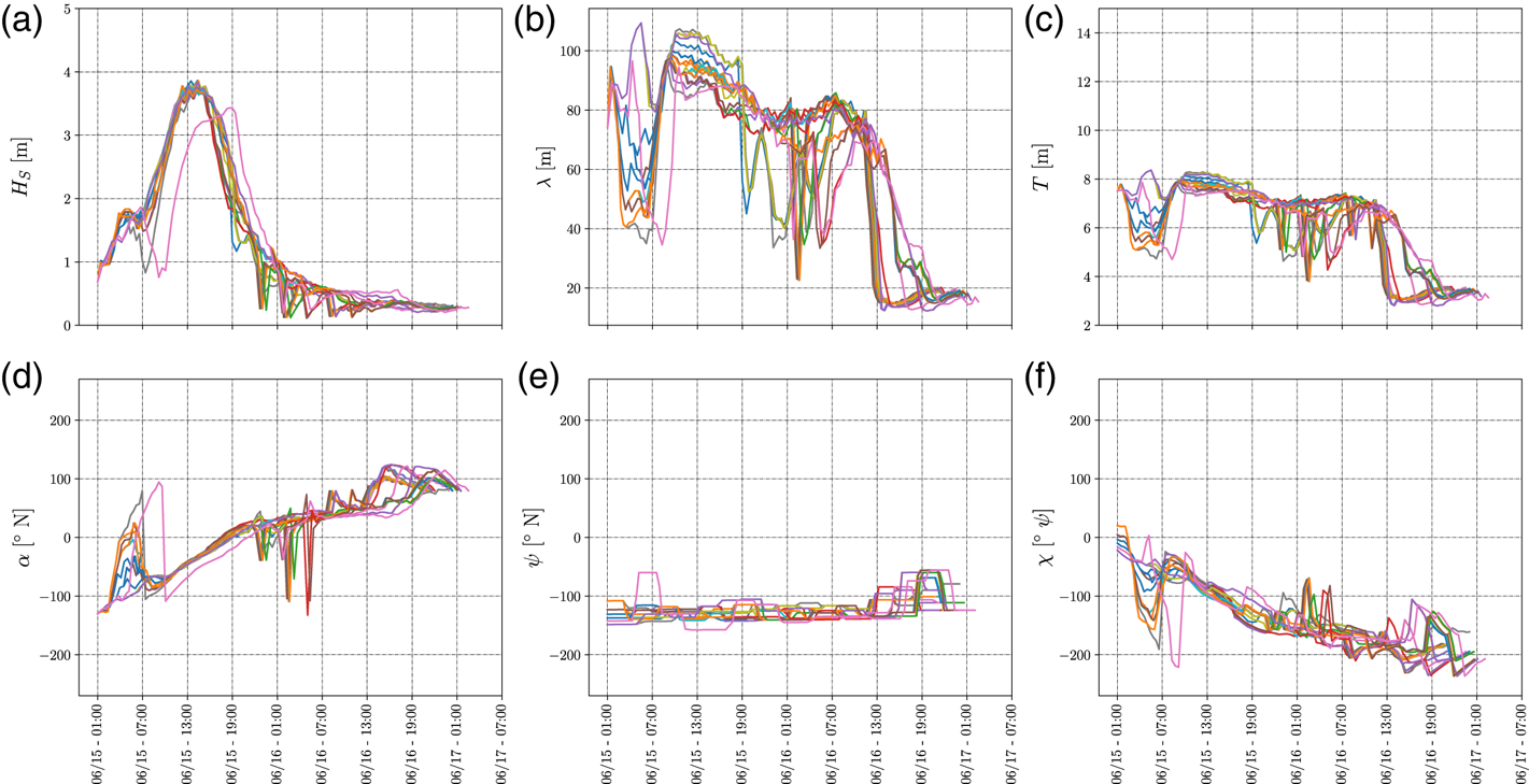
Figure 11. High operational safety OTW–METOC conditions of the routes identified by high operational safety in the travel time window ETD June 15th, 2018, [01:00–04:00] UTC and ETA June 16th, 2018, [17:00–23:00] UTC. The sub-figures represent: (a) the significant wave height $H_S$ ; (b) the mean wave peak period $T$
 ; (c) the mean wavelength $\lambda$
 according to IMO (2007); (d) the mean wave direction $\alpha$
 ; (e) the heading of the ship $\psi$
 ; (f) the wave encounter angle $\chi$
 (with respect to the heading of the ship)
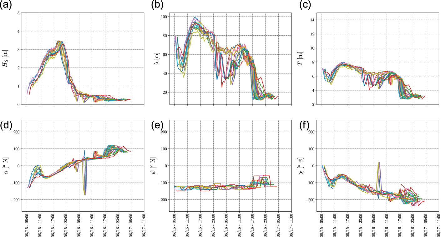
Figure 12. High operational safety OTW–METOC conditions of the routes identified by high operational safety in the travel time window ETD June 15th, 2018, [05:00–07:00] UTC and ETA [June 16th, 2018, 21:00–June 17th, 2018, 01:00] UTC. The sub-figures represent: (a) the significant wave height $H_S$ ; (b) the mean wave peak period $T$
 ; (c) the mean wavelength $\lambda$
 according to IMO (2007); (d) the mean wave direction $\alpha$
 ; (e) the heading of the ship $\psi$
 ; (f) the wave encounter angle $\chi$
 (with respect to the heading of the ship)
Figure 10 shows that the Pareto-optimal routes are characterised by waves with $H_S$ up to $5$
 m, $T$
 up to $9$
 s and $\lambda$
 up to $130$
 m (estimated through the Hunt method (U.S. Army Engineer Waterways Experiment Station, Coastal Engineering Research Center, 1985)). These sea conditions may produce dangerous sailing conditions according to IMO (IMO, 2007). Such effects are reduced in the high operational safety interval, which presents lower waves with $H_S \approx 3{\cdot }5$
 m, as depicted in Figure 11. The exposure to severe METOC conditions decreases by delaying the departure by an additional hour. This arises from the high density of high (violet) operational safety cells in the OTW with ETD in the interval June 15th, 2018, [05:00–07:00] UTC with ETA in the interval [June 16th, 2018, 21:00–June 17th, 2018, 01:00] UTC, as depicted in Figure 12, where waves with $H_S \approx 3{\cdot }5$
 m are present. The other OTW are characterised with medium/marginal operational safety for the execution of operations.
The proposed approach presents the advantages of automating the process of selecting the best OTW from a safety point of view by considering a set of Pareto optimal routes available for a temporal window covering $16$ h (in our case of study $16$
 h, but could be of a different duration). The decision maker can explore the reduced set of routes available for an identified OTW and have an overview of the average sailing conditions for the selected temporal window. Starting from the OTW, new runs of the weather routing process can be executed. These runs are setup at higher spatial resolution with updated constraints in terms of ETD–ETA (identified from the OTW). At this stage, the decision maker could explore the new reduced set of Pareto-optimal routes. The selection of the final route relies on the experience and additional evaluations of a trained decision maker. To support the decision maker in the selection of the best trade-off route, different methodologies are available. These aspects are beyond the scope of this paper. As reference, we recall the publications of Fabbri and Vicen-Bueno (Reference Fabbri and Vicen-Bueno2019), Chiu and Bloebaum (Reference Chiu and Bloebaum2009) (and references therein) that cover the route selection process.
5. Conclusions
A new decision layer within a general weather routing system has been proposed with the aim to support decision makers and navigators during the planning of ship operations. The contribution provides a methodology for the analysis of the routes computed by any weather routing system by means of the guidelines defined by the IMO (IMO, 2007) and the operational safety metric derived.
The presented simulations demonstrate how the proposed decision layer is able to identify the optimal ETD–ETA window of opportunity to execute a particular ship operation (e.g. travel/transit) based on the METOC conditions and the derived sailing conditions. The proposed OTW representation is able to visualise, in a user-friendly manner, the ETD–ETA windows of opportunity with associated high, medium and low operational safety conditions to run a ship operation. This allows a decision maker to execute a preliminary assessment of the routes proposed by any weather routing system and afterwards execute a higher resolution weather routing process in a restricted time window (e.g. select a given route from those proposed). Furthermore, the proposed solution allows the decision maker to interact with the system by providing a custom configuration based on the type of mission scenario.
The concept presented in this paper represents a proof-of-concept requiring further development to reach the state of a usable tool by the decision maker. Future works will be focused on the experimentation of the tool in real-case scenarios. Furthermore, the incorporation of the IMO second generation intact stability criteria (Papanikolaou et al., Reference Papanikolaou, Vassalos, Hamamoto and Molyneux2000; Neves et al., Reference Neves, Belenky, Kat, Spyrou and Umeda2011; Peters et al., Reference Peters, Belenky, Bassler, Spyrou, Umeda, Bulian and Altmayer2011; Masoudi, Reference Masoudi2017) and the concept of climate wave spectrum (Degtyarev et al., Reference Degtyarev, Boukhanovsky, Lopatoukhin and Rozhkov2000; Boukhanovsky et al., Reference Boukhanovsky, Lopatoukhin and Soares Guedes2007) could be exploited to improve the idea of OTW.
Acknowledgment
This work has been funded by the Defence Research and Development Canada (DRDC) under the project ‘Mission Planning Aid - Decision Support and Risk Assessment’ (MPA-DeSRA). The project has been developed in collaboration with the Environmental Knowledge and Operational Effectiveness/Maritime Intelligence Surveillance and Reconnaissance (EKOE/MISR) programme at the NATO STO Centre for Maritime Research and Experimentation (CMRE). The authors also thank the DICCA-MeteOcean Department (Dipartimento di Ingegneria Civile, 2018) for providing the METOC forecast data for the scenario.


