PRESIDENTIAL ELECTIONS

The presidential election model is written thusly (Lewis-Beck and Rice Reference Lewis-Beck and Rice1984a, 17):

(Eq.1) $$ \mathrm{Incumbent}\ \mathrm{Vote}=\mathrm{Presidential}\ \mathrm{Popularity}+\mathrm{Economic}\ \mathrm{Growth}, $$

where the Presidential Vote = the two-party share of the national popular vote for the president’s party, Economic Growth = the GNP growth in the first two quarters of the election year, and Presidential Popularity = Gallup’s July job approval rating for the president.

According to the model, the election represents a referendum on the performance of the president with respect to leading political and economic issues. The better the performance, the better the White House party will do. Below we show model estimates using ordinary least squares (OLS):

(Eq. 2) $$ {\displaystyle \begin{array}{l}\mathrm{Vote}=37.50+.26\ast \mathrm{Popularity}+1.18\ast \mathrm{Growth}\\ {}\quad (15.37)\quad (4.73)\quad (2.25)=\mathrm{t}-\mathrm{ratio}\end{array}} $$

R-squared = .76 Adj. R-squared = .73 Root Mean Squared Error = 2.75 Durbin-Watson = 2.39 N = 18 elections, 1948-2016 Figures in parentheses = t-ratios Asterisk indicates statistical significance = .05, one-tail (Tien Reference Tien2020).

This model, though parsimonious, forecast the 2016 result quite accurately. Indeed, it nailed the two-party popular vote result, forecasting a 51.0 percentage share for Clinton, who actually received 51.1% (Lewis-Beck and Tien Reference Lewis-Beck and Tien2018). This trivial amount of error gave the model first place, in an accuracy evaluation of such structural forecasting models (Campbell Reference Campbell2017). While it would be foolish optimism to expect such a degree of accuracy in 2020, it seems reasonable to believe the model will fare well with respect to the Trump-Biden contest. To forecast 2020, we insert the current values as of 8/27/20 for the predictor variables, Popularity (41) and Growth (-4.14)Footnote ¹ :

(Eq.3) $$ {\displaystyle \begin{array}{l}\mathrm{Vote}=37.50+.26\ (41)+1.18\ \left(-4.14\right)\\ {}\quad =43.3\%\quad \mathrm{of}\ \mathrm{the}\ \mathrm{popular}\ \mathrm{two}-\mathrm{party}\ \mathrm{vote}\ \mathrm{for}\ \mathrm{Trump}.\end{array}} $$

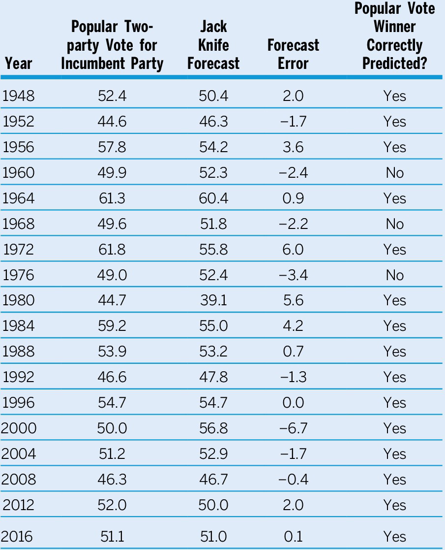
How accurate do we expect this forecast to be? First, over the time series of elections, it correctly picked the winning party 15 out of 18 times (missing 1960, 1968, and 1976), or 83% of the time. This certainty speaks to within-sample error. To examine out-of-sample error, we ran a series of jackknife tests (see table 1). That is, taking each year in turn, we dropped it from the data, re-estimated the model, then predicted that out-of-sample year and examined the forecasting error. We found zero elections with a positive error greater than 6.7%. Since our forecast is 43.3, if it has an error greater than +6.7, we would forecast a victory for the wrong party. Taken literally, that would leave no chance that this forecast of a Democratic victory would be wrong (i.e., 0/18 = .00). We shy away from such a high level of certainty. However, we construct the following 95% confidence interval (two-tail) around our point estimate of 43.3, utilizing the RMSE=2.75 and degrees of freedom=15 : [37.41, 49.6]. This result suggests a 95% probability that Trump will lose the popular vote. Twice in the last five presidential elections, the Electoral College, and not the popular vote outcome, picked the presidential winner. Thus, we forecast the Electoral College winner by regressing the incumbent party’s percent of the Electoral College vote on its percent of the two-party popular vote. We get the following results

(Eq. 4) $$ {\displaystyle \begin{array}{l}\mathrm{EC}\ \mathrm{Vote}=-199.42+4.90\ast \mathrm{PopVote}\\ {}\quad \left(-11.64\right)\quad (14.94)=\mathrm{t}-\mathrm{ratio}\\ {}\mathrm{R}2=.93\quad \mathrm{adj}\ \mathrm{R}2=.93\quad \mathrm{N}=18\quad \mathrm{R}\mathrm{MSE}=7.14\end{array}} $$

Table 1 Presidential Election Predictions with the Political Economy Model

This equation yields an Electoral College forecast of only 68 electoral votes for Trump. Interestingly, this is on par with Jimmy Carter’s defeat in 1980 with 49 electoral votes.

One may be skeptical of this dramatic forecast. However, we note that 1980 happens to be the election year in our series with the most negative GNP growth. One could argue, more generally, that times are very different now and the popular vote-electoral vote connection has broken down. However, in a statistical sense, that conclusion has clay feet. In figure 1 we see the Electoral College vote share nationwide (in percent) regressed on the two-party popular vote, for the elections from 1948 to 2016. The election results fall very close to the prediction line, with an almost perfect statistical fit (R-squared = 0.93). Further, we do not really observe a deterioration in the fit when we focus on the elections of the 2000s. (Look how close the points are to the line, with even 2016 closer than some previous elections.)

Figure 1 Electoral College Vote by Popular Vote, 1948-2016

CONGRESSIONAL ELECTIONS

Forecasts for the United States House and Senate elections have been carried out from the early 1980s (Lewis-Beck and Rice Reference Lewis-Beck and Rice1984b; Reference Lewis-Beck and Rice1985). These models rest on a core political economy model:

(Eq.5) $$ \mathrm{House}\ \mathrm{Seat}\ \mathrm{Change}=\mathrm{Presidential}\ \mathrm{Popularity}+\mathrm{Income}\ \mathrm{Growth}+\mathrm{Midterm}\ \mathrm{Status}, $$

with House Seat Change = number of seats lost or gained by the president’s party, Presidential Popularity = Gallup’s June job approval rating for the president, economic conditions = growth rate of real disposable income over the first two quarters of the election year, Midterm Status = 0 for presidential election years and = 1 for midterm election years.

For House forecasts, we use a simple referendum model, conditioned on whether the contest is a midterm. In the most recent House election, 2018, this model performed quite well, with a total seats change error of only nine seats, well below the median error for the series (Tien and Lewis-Beck Reference Tien and Lewis-Beck2019). Given we are in a presidential year, White House success in terms of making seat gains (or losses) boils down to how the Republicans have handled economic and non-economic issues. OLS estimates for the post-World War II elections follow:

(Eq. 6) $$ \mathrm{House}\ \mathrm{Seat}\ \mathrm{Change}=-45.53+.83\ast \mathrm{Popularity}+4.89\ast \mathrm{Income}\hbox{--} 29.1\ast \mathrm{Midterm}(-3.55)\quad (3.47)\quad (2.95)\quad (-4.81)=\mathrm{t}-\mathrm{ratio} $$

R-squared = .60 Adj. R-squared = .57 Root mean squared error = 17.85. Durbin-Watson = 1.87, N = 36 elections (1948-2018) and the other notation is as with Eq.2.

To use this equation to forecast the 2020 House elections, we plug in the appropriate values (as of 7/27/20),Footnote ² so producing the following seat change estimate:

(Eq. 7) $$ {\displaystyle \begin{array}{l}\mathrm{House}\ \mathrm{Seat}\ \mathrm{Change}=-45.53+.83\ (38)+4.89\ \left(-3.77\right)-29.1\ (0)\\ {}\quad =-32\ \mathrm{seat}\ \mathrm{loss}\ \mathrm{for}\ \mathrm{the}\ \mathrm{Republicans}.\end{array}} $$

What about seat change for the 2020 Senate elections? We hold that the political economic forces operating on the House also operate on the Senate, with the added constraint of their different electoral calendar (i.e., just one-third of the Senate seats are on the ballot, every two years). The Senate forecasting model expresses itself as:

(Eq.8) $$ \mathrm{Senate}\ \mathrm{Seat}\ \mathrm{Change}=\mathrm{Popularity}+\mathrm{Economy}+\mathrm{Midterm}+\mathrm{Seats}\ \mathrm{Exposed}, $$

with Senate Seat Change = number of seats lost or gained by the president’s party; Seats Exposed = number of seats the president’s party has up for reelection; the other variables are as defined in equation 5. Here are OLS estimates for the model, across the post-World War II elections:

(Eq. 9) $$ \mathrm{Senate}\ \mathrm{Seat}\ \mathrm{Change}=2.79+.13\ast \mathrm{Popularity}+.91\ast \mathrm{Income}\hbox{--} 2.37\ast \mathrm{Midterm}-.70\ast \mathrm{Seat}\mathrm{s}\mathrm{Up}(1.05)(3.46)(3.35)(-2.44)(-6.42)=\mathrm{t}-\mathrm{ratio} $$

R-squared = .69 Adj. R-squared = .65 Root mean squared error = 2.84 Durbin-Watson = 1.86, N = 36 elections (1948-2018) and the other notation is as with Eq.2. All independent variable coefficients are statistically significant at the 0.05 level, one-tail.

What does this mean for Senate control in 2020? Trump’s June approval rating is 38%, disposable personal income change has been strongly negative (at -3.77), and the Republicans have 23 seats exposed (using data reported as of 7/27/20). These numbers forecast a gain of 12 seats for the Democrats, giving Democrats a Senate majority.