


1. INTRODUCTION
With the increasing demand of marine exploration and the development of seabed topographic mapping methods (such as bathymetry systems), a significant amount of work has been done to produce high-resolution maps of the seabed (Doble et al., Reference Doble, Forrest, Wadhams and Laval2009; Wang et al., Reference Wang, Lv, Zhang, Liu and Er2017a). However, because the map resolution for shipborne bathymetry systems is proportional to the water depths, shipborne bathymetry systems cannot not meet the requirements of high-resolution mapping in deep waters. Due to their ability to operate close to the seafloor regardless of depth, Autonomous Underwater Vehicles (AUVs) have become important mapping platforms for topography missions and geological surveys such as searching for manganese nodules, hydrothermal vents and remains of vessels.
The accuracy of a bathymetric map depends on the accuracy of navigation of the AUV. Global Navigation Satellite Systems (GNSSs), Dead Reckoning (DR), Ultrashort-Baseline (USBL), and Long-Baseline (LBL) acoustic positioning systems all provide options for improving navigational accuracy, with various levels of attainable precision (Paull et al., Reference Paull, Saeedi, Seto and Li2014). GNSS observations can provide accurate locations, but this requires the AUV to surface. DR navigation error is related to the total distance travelled, which means it is unsuitable for a long-term underwater navigation scenario without other precise auxiliary means of positioning. Although USBL and LBL could provide a bounded navigation error, support vessels or acoustic arrays are necessary, and this would limit the operating range of the AUV.
As a more recently developed approach to provide accurate navigation solution for AUVs without any aids, the Simultaneous Localisation And Mapping (SLAM) technique has been introduced. The SLAM technique makes it possible for a vehicle to incrementally build a map of an unknown environment with consistency while simultaneously determining its location within this map (Durrant-Whyte and Bailey, Reference Durrant-whyte and Bailey2006). Many breakthroughs in the development of the SLAM technique have been made in Unmanned Ground Vehicles (UGVs) (Ila et al., Reference Ila, Polok, Solony and Svoboda2017; Dellaert and Kaess, Reference Dellaert and Kaess2006) and Unmanned Aerial Vehicles (UAVs) (Kownacki, Reference Kownacki2016). Underwater SLAM algorithms for AUVs have also been developed, and most of them are applied using a camera (Kim and Eustice, Reference Kim and Eustice2013), a mechanically scanned imaging sonar (Mallios et al., Reference Mallios, Ridao, Ribas and Hernández2014; Ribas et al., Reference Ribas, Ridao, Tardós and Neira2008) and Forward-Looking Sonar (FLS) (Hurtós et al., Reference Hurtós, Ribas, Cufí, Petillot and Salvi2015; Johannsson et al., Reference Johannsson, Kaess, Englot, Hover and Leonard2010). However, the use of a camera is limited to applications in which the vehicle navigates in clear water and very near to the seafloor (Ribas et al., Reference Ribas, Ridao, Tardós and Neira2008), and SLAM techniques with mechanically scanned imaging sonars cannot be applied in unstructured environments. As imaging the same scene from two different vantage points can cause significant alterations in the measurement, the forward-looking sonar SLAM can only register images that differ in small orientations, and this makes it difficult to obtain loop closures (Hurtós et al., Reference Hurtós, Ribas, Cufí, Petillot and Salvi2015). Compared with the techniques listed above, Bathymetric SLAM (BSLAM) is more flexible and has little restriction in terms of water clarity, environment and vantage points. The major limitation of BSLAM is that the best navigation results can only be provided when the depth profile of the seabed varies significantly (Barkby et al., Reference Barkby, Williams, Pizarro and Jakuba2009). However, with a prior bathymetric map with a much lower resolution (such as a map resolution of 500 metres), it is possible to calculate the corresponding terrain information such as the terrain entropy and choose some areas which satisfied the entropy condition (for one area including 20×20 points, its entropy should be no less than two according to Feng (Reference Feng2004)) to conduct the BSLAM process as a benchmark, while the remaining areas could be mapped via topographic expansion surveys. Accordingly, building a bathymetric map and then simultaneously locating using it is more reliable than the above techniques using vision, mechanically scanned imaging sonar, or forward-looking sensors in most cases.
BSLAM has received great attention. Barkby et al. (Reference Barkby, Williams, Pizarro and Jakuba2012) proposed a Bathymetric Particle filter SLAM (BPSLAM) to help locate the position of the AUV in real time without loop detection. This algorithm applied a Gaussian process and a Rao–Blackwellized particle filter to calculate SLAM solutions, and an ancestry tree was used to reduced computation. Regrettably, the computational efficiency of the BPSLAM still limits its real-time performance. Palomer et al. (Reference Palomer, Ridao, Ribas, Mallios, Gracias and Vallicrosa2013) improved the Extended Kalman Filter (EKF) SLAM using an octree-established point-cloud sampling model and applied an Iterative Closest Point (ICP) algorithm for terrain matching. However, this method can only correct the overall position of each submap and the location errors within the submap were neglected. Roman and Singh (Reference Roman and Singh2010) proposed a SLAM method including map registration and pose filtering, and experiment results have shown its significant improvements in map quality. In addition, within the loop closures detection technique in BSLAM, a terrain matching technique has also been developed over a long period and has now been applied successfully in AUVs (Ånonsen et al., Reference Ånonsen, Hagen, Hegrenæs and Hagen2013). For example, based on a Particle Filter (PF), Donovan (Reference Donovan2012) proposed a Three-Dimensional (3D) terrain matching method considering tide correction and presented a novel PF-resampling technique to consistently recover a position fix over a search area of several kilometres without significantly increasing the number of particles used, and also proved the algorithm's robustness.
Until recently, some difficulties have not been fully solved in BSLAM. They include the obvious overlap of the bathymetric data that could not be obtained for adjacent time periods, and this makes it difficult to measure the inter-frame motion. Also, loop closures obtained by terrain matching have a great impact on navigation results. Navigation results for vehicles are inaccurate if inaccurate loop closures cannot be identified.
To overcome these difficulties, the BSLAM algorithm based on the graph method is proposed. To estimate the inter-frame motion, the BSLAM algorithm constructs weak data association by comparing prior estimation and measurement, and estimation is obtained by a maximum likelihood terrain estimation approach. A weighted voting method for the loop closures has also been proposed to identify inaccurate loop closures. In contrast to the filter BSLAM methods proposed by Barkby et al. (Reference Barkby, Williams, Pizarro and Jakuba2012) and Palomer et al. (Reference Palomer, Ridao, Ribas, Mallios, Gracias and Vallicrosa2013), our proposed algorithm does not need to make strong assumptions of state transfer and measurement functions, and this means the modelling errors caused by hydrodynamic force coefficients and complex measurement noise would have little impact on the BSLAM solutions. Meanwhile, the BSLAM algorithm calculates a posterior probability over the entire path along with the map instead of just the current pose-like filter methods (Thrun et al., Reference Thrun, Burgard and Fox2005).
An experiment using a shipborne bathymetry system was conducted. On board data was collected, including an 8 km planned track recorded at 4 knots, and a high-resolution bathymetric map of around 0·56 km2 was built. Using this data, a playback experiment was conducted to verify the validity and real-time performance of the BSLAM algorithm, and the experiment results verified the viability, accuracy and real-time performance of the BSLAM.
The rest of paper is organised as follows. An overview of the BSLAM algorithm is introduced in Section 2. A description of the graph construction algorithm is given in Section 3. The graph optimisation algorithm is proposed in Section 4 and the playback experiment and its results are discussed in Section 5. Finally, the conclusions are given in Section 6.
2. OVERVIEW OF THE BSLAM ALGORITHM
Similar to graph SLAM, the BSLAM algorithm also consists of both graph construction and optimisation. In the graph construction, the trajectory of the AUV is divided into various submaps, and loop closures between submaps are detected. AUV motion between adjacent frames is estimated via weak data association. Meanwhile, all loop closures are identified via the weighted voting method, and then the pose graph is built using AUV states, odometry constraints, weak data associations and loop closures. In the graph optimisation process, all frames associated with loop closures are named as key frames. AUV states on key frames are corrected via global trajectory correction and all of the rest states are modified in the local trajectory correction process. The main BSLAM framework is shown as Algorithm 1.
Algorithm 1 BSLAM FRAMEWORK

As shown in Algorithm 1, the main steps of the BSLAM are:
(1) Graph Construction (Line 2 to 6 in Algorithm 1):
(a) The navigation and bathymetric data is obtained via the DR and bathymetry systems, respectively, and they are divided into various submaps; (Section 3.1)
(b) Weak data association construction; (Section 3.2)
(c) Loop closures between the current submap and all historical submaps are detected by terrain matching technique, and inaccurate loop closures can be identified via a weighted voting method; (Section 3.3)
(2) Graph Optimisation (Line 8 to 9 in Algorithm 1):
(a) Combined with the loop closures and weak data association, the purpose of the global trajectory correction is to find the solution of the SLAM least squares problems. (Section 4.2.1)
(b) After obtaining the global trajectory correction results, local trajectory correction modifies the local trajectory with the aid of weak data association. (Section 4.2.2)
Moreover, in the BSLAM process, the vehicle track is designed to achieve the best results from both vehicle navigation and topographic mapping. As shown in Figure 1, our planned track for the AUV looks like a Chinese knot to obtain more loop closures. Later, we adopted this track pattern during the experiment, and results show the BSLAM algorithm performs well when using this track.

Figure 1. Planned track of the BSLAM process.
3. GRAPH CONSTRUCTION
The purpose of graph construction is to build the pose graph. As shown in Figure 2, the pose graph of the BSLAM consists of the vehicle states (![]() ), odometer constraints (
), odometer constraints (![]() ), weak data association (
), weak data association (![]() ) and loop closures (
) and loop closures (![]() ). The odometer constraint
). The odometer constraint ![]() can be obtained from the navigation system, and the weak data association
can be obtained from the navigation system, and the weak data association ![]() is obtained using maximum likelihood terrain estimation. The loop closure
is obtained using maximum likelihood terrain estimation. The loop closure ![]() is detected by terrain matching techniques, and this closure is also called a loop closing constraint (Rosen et al., Reference Rosen, Kaess and Leonard2012).
is detected by terrain matching techniques, and this closure is also called a loop closing constraint (Rosen et al., Reference Rosen, Kaess and Leonard2012).
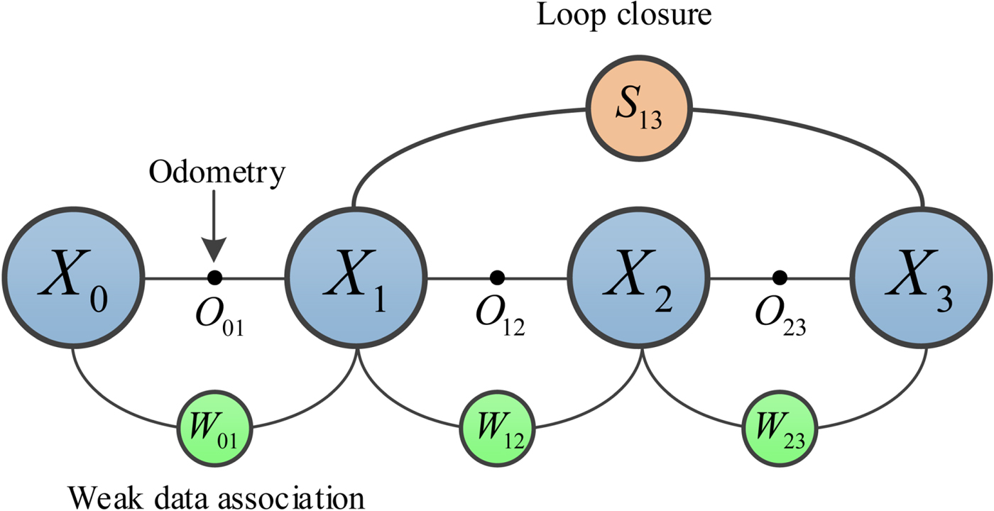
Figure 2. Schematic diagram of pose graph construction.
3.1. Generation of submaps
In BSLAM, the first and most basic step is to log bathymetric data. The bathymetric data can be obtained by combining the Two-Dimensional (2D) swaths from a bathymetry system and vehicle trajectory from a DR system.
As shown in Figure 3, for one measurement point in the 2D swath, the bathymetry system would return the beam length r and the echo angle β. The corresponding trajectory point is  $X=(x,y,z,\varphi,\theta,\psi)$, where x, y, z are the position in XG (east), YG (north) and SG (vertical) -axes in a geodetic coordinate system, and φ, θ, ψ denote the rotation around XG, YG and ZG -axes, respectively. Combined with the trajectory data, the corresponding bathymetric data
  $X_{M}=(x_{M},y_{M},z_{M})$ in the geodetic coordinate system can be obtained via Equation (1):
 $$\begin{align} &\left[\begin{matrix} x_{M}\\ y_{M}\\ z_{M}\\ 1 \end{matrix}\right]=R\left[\begin{matrix} 0\\ r\sin\beta\\ r\cos\beta\\ 1 \end{matrix}\right]\\ &\hbox{where}\\ & R=\left[\arraycolsep3pt\begin{matrix} \cos\theta\cos\psi+\sin\varphi\sin\theta\sin\psi & \cos\varphi\sin\psi & -\sin\theta\cos\psi+\sin\varphi\cos\theta\sin\psi & x\\ -\cos\theta\cos\psi+\sin\varphi\sin\theta\sin\psi & \cos\varphi\cos\psi & -\sin\theta\sin\psi+\sin\varphi\cos\theta\cos\psi & y\\ \sin\theta\cos\psi & -\sin\varphi & \cos\theta\cos\psi & z\\ 0 & 0 & 0 & 1 \end{matrix}\right] \end{align}$$
Figure 3. The measurement model of the AUV (a) Measurement model (b) 2D measurement model.
It must be noted that, due to the measurement errors of a bathymetry system, noise would affect the bathymetric data and some outliers would be produced. To deal with this problem, the automatic processing algorithm proposed by Chen (Reference Chen2016) is applied to detect the outliers of bathymetric data in the process of bathymetric data acquisition. This algorithm uses the Alpha-Shapes model to detect the outliers in 2D swaths efficiently, and its viability and accuracy have been proved with both flat and complex terrain. In addition, although systematic errors of attitude and heading would also influence the bathymetric data, these impacts are negligible because the measurement error of the Fibre Optic Gyrocompass (FOG) used in this paper is less than 0·1°.
During the topographic mapping mission, the trajectory and the corresponding bathymetric data is constantly divided into various submaps considering the time-consumption problem (Palomer et al., Reference Palomer, Ridao and Ribas2016). Submaps are created on the basis of the trajectory length and the amount of information in the bathymetric data. The minimum and maximum lengths of the submap are set according to the actual situation. Considering the amount of information in the bathymetric data, Palomer et al. (Reference Palomer, Ridao, Romagós and Vallicrosa2015) proposed a method using DoN to identify the object when the measurement noise is not only considerably high, but also more scattered. DoN provides a multi-scale approach to process large unorganised Three-Dimensional (3D) point clouds for detecting the areas where the point cloud has significant changes, and it has been proven to be a computationally efficient method. Thus, in this study, DoN is introduced to represent the amount of information in bathymetric data, and the DoN value in measurement point i can be calculated as:
 $$\Delta\hat{n}_i(p,r_1,r_2)=\frac{\hat{n}_i(p,r_1)-\hat{n}_i(p,r_2)}{2}$$
where,  $\Delta\hat{n}_{i}(p,r_{1},r_{2})$ represents the DoN value, p denotes the point cloud of bathymetric data.
  $\hat{n}_{i}(p,r_{1})$ and
  $\hat{n}_{i}(p,r_{2})$ are the normal with support radius r 1 and
  $r_{2}(r_{1}<r_{2})$ at time I, and they are estimated by finding the tangent plane using the principal components of the points lying within a sphere of a fixed support radius. In this paper, we define the DoN value of one submap includes n measurement points as:
 $$\textit{DoN}=2{\cdot}\sum_{i=1}^n don_i$$
where:
 $$don_i=\begin{cases} 1 & \Delta\hat{n}_i(p,r_1,r_2)>0{\cdot}5\\ 1 & \Delta\hat{n}_i(p,r_1,r_2)\leq 0{\cdot}5\\ \end{cases}$$
An increase in the DoN value means a clear change in the terrain is observed. When the DoN value of current submap is higher than the threshold and the minimum patch size has been reached, the current submap is stored and a new submap is started (Roman and Singh, Reference Roman and Singh2010).
3.2. Weak data association
While obtaining and storing the bathymetric data, weak data association at adjacent time periods is constantly built to estimate the inter-frame motion. The weak data association is the likelihood that the measurement matches the prior estimation, and this can be calculated by a comparison of the measurement and a prior estimation of it.
As shown in Figure 3, the measurement model of bathymetry system at time i is:
 $$Z_i^+=h(X_i)+e_i$$
where Z i+ is measured terrain elevation, and e i denotes measured noise of bathymetric data with a distribution of  ${\rm N}(0,0{\cdot}4)$ according to the parameter of GS+ wide-swath bathymetry system used in this paper.
The prior estimation can be obtained with a maximum likelihood terrain estimation algorithm we have previously proposed, called the Terrain Elevation Measurement Extrapolation Estimation (TEMEE) (Li et al., Reference Li, Ma, Wang, Chen and Zhang2017). By combining the historical data including  $X_{i-n}, Z_{i-n}^+, \ldots, Z_{i-1}^+$, and the current vehicle state X i, the estimated measurement Z i− can be obtained via the TEMEE algorithm. The details of the prior estimation are long and therefore omitted here for brevity.
Then the weak data association between time i−1 and i can be expressed as:
 $$\begin{align} \textit{likelihood}&=p(X_i\vert X_{i-1})\propto p(Z_{i}^+-Z_{i}^-)\\ &=\frac{1}{\sqrt{(2\pi)^N\det(\textbf{C}_e)}}\exp\left(-\frac{1}{2}(Z_{i}^+-Z_{i}^-)^T\textbf{C}_e^{-1}(Z_{i}^+-Z_{i}^-)\right)\\ &=\frac{1}{(2\pi\sigma_e^2)^{N/2}}\exp\left(-\frac{1}{2\sigma_e^2}\sum_{k=1}^N(Z_i^+[k]-Z_i^-[k])^2\right) \end{align}$$
where  $\textbf{C}_{e}=\textit{diag}(\sigma_{1}^{2},\sigma_{2}^{2},\sigma_{1}^{3},\ldots,\sigma_{k}^{2})$ is a diagonal matrix consisting of the variance components of each sampling point, N represents the number of measurement points and Z[k] is the elevation of the k-th measurement point. As the measurements of all the sampling points are considered independent of the others, assuming that measurement variance is the same in all beams, we can simply make
  $\textbf{C}_{e}=\sigma_{e}^{2}\textbf{I}$ and
  $\sigma_{e}^{2}=0{\cdot}4$ according to e i in Equation (5) (Nygren, Reference Nygren2005).
3.3. Loop closure detection
3.3.1. Terrain matching
Different from weak data association, loop closures have a high confidence level and they are detected by terrain matching techniques between submaps. Whenever a new submap is stored, the terrain matching procedure runs between the current submap and all the historical submaps in its search circle. The radius of the circle is the maximum navigation error in the current submap.
As shown in Figure 4, it is assumed that submap 1 is in the search circle of submap 2, then submap 2 would be divided into match units as shown in Figure 4, and each match unit looks for the most similar area in submap 1. For match unit unit_k; in submap 2 and all M match units in submap 1, the likelihood function L k is given as follows:
 $$L_k=\max\left(\frac{1}{(2\pi\sigma_g^2)^N}\exp\left(-\sum_{n=1}^N(unit\_k_n-unit\_l_n)^2/2\sigma_g^2\right)\right)\quad (l=1,2,3,\ldots,M)$$
where σg represents the covariance matrix of the measurement noise in the grid map (Zhou et al., Reference Zhou, Cheng, Zhu, Dai and Fu2017), but here it could be calculated as the average residual of the match unit, as well as N is the same as the corresponding values in Equation (6). If L k is more than the matching-threshold, the terrain information would judge the correctness of the matching result. Here the terrain entropy is applied to represent the terrain information because it is insensitive to measurement noise. In the map with elevation value h(i, j) at (i, j), terrain entropy H T can be described as:
 $$\begin{cases} P(i,j)=\dfrac{h(i,j)}{\sum_{i=1}^m\sum_{j=1}^n h(i,j)}\\ H_T=\dfrac{1}{mn}\sum_{i=1}^m\sum_{j=1}^nP(i,j)\ln[P(i,j)] \end{cases}$$
Figure 4. Calculation of confidence.
Making m and n equal to 20, if the current terrain information H T is no less than 2, this matching result is valid and we denote the corresponding loop closure as l k (Feng, Reference Feng2004). Finally, to reduce the computation, only one loop closure l 1 with maximum likelihood function is retained in one matching procedure. The number of other loop closures which have the same value or slight difference with l 1 is used to express the reliability of this retained loop closure.
3.3.2. Weighted voting method
In the marine environment, the bathymetric data is influenced by the vehicle pose, reverberation and other environmental characteristics, and it can result in inaccurate loop closures (Nygren and Jansson, Reference Nygren and Jansson2004; Wang et al., Reference Wang, Su, Yin, Zheng and Meng2017b). If the inaccurate loop closures cannot be identified for a long time, the effectiveness of the BSLAM algorithm will be significantly affected. Thus, a weighted voting method is proposed to judge whether the loop closures are accurate.
In this method, each loop closure provides scores for each of the remaining closures in the survey process according to the corresponding combination of these two closures.
As shown in Figure 5, there are three kinds of possible networks for the combinations. ![]() is the vehicle state, and the black line connecting state X i and X j describes the loop closure with value
is the vehicle state, and the black line connecting state X i and X j describes the loop closure with value  $D_{ij}^{S}$ and information matrix
  $S_{ij}^{-1}$, and the black dotted line connecting the same states denotes the odometer constraint with value
  $D_{ij}^{o}$ and information matrix
  $O_{ij}^{-1}$.

Figure 5. Network of combination of two loop closures (a) Network 1 (b) Network 2 (c) Network 3.
For Network 1, the derived estimates of X 3 and its information matrix  $C_{3}^{-1}$ are:
 $$\begin{align} X_3&=(S_{01}^{-1}+O_{01}^{-1})^{-1}(S_{01}^{-1}D_{01}^{s}+O_{01}^{-1}D_{01}^{o})+D_{12}^o +(S_{23}^{-1}+O_{23}^{-1})^{-1}(S_{23}^{-1}D_{23}^{s}+O_{23}^{-1}D_{23}^{o})\\ C_3^{-1}&=[(S_{01}^{-1}+O_{01}^{-1})^{-1}+O_{12}+(S_{23}^{-1}+O_{23}^{-1})^{-1} \end{align}$$
For Network 2, the corresponding values are:
 $$\begin{align} C'_{0123}&=O_{01}+(S_{12}^{-1}+O_{12}^{-1})^{-1}+O_{23}\\ D'_{0123}&=D_{01}^o+(S_{12}^{-1}+O_{12}^{-1})^{-1}(S_{12}^{-1}D_{12}^{s}+O_{12}^{-1}D_{12}^{o})+D_{23}^o\\ X_{3}&=(C_{0123}^{\prime -1}+S_{03}^{-1})^{-1}(C_{0123}^{\prime -1}D'_{0123}+S_{03}^{-1}D_{0123}^s)\\ C_3^{-1}&=C_{0123}^{\prime -1}+S_{03}^{-1}. \end{align}$$
 Network 3 is in the form of a Wheatstone bridge, the variables X 3 can be solved from the linear system GX=B where  ${\rm X}=\{X_{1},X_{2},X_{3}\}$:
 $$\begin{align} \hbox{G}&=\left[\begin{matrix} O_{01}^{-1}+O_{12}^{-1}+O_{23}^{-1} & -O_{12}^{-1} & -S_{13}^{-1}\\ \noalign{\vskip3pt} -O_{12}^{-1} & S_{02}^{-1}+-O_{12}^{-1}+-O_{23}^{-1} & -O_{23}^{-1}\\\noalign{\vskip3pt} -S_{13}^{-1} & -O_{23}^{-1} & -S_{13}^{-1}+-O_{23}^{-1} \end{matrix}\right]\\ \hbox{B}&=\left[\begin{matrix} O_{01}^{-1}D_{01}^o+O_{12}^{-1}D_{12}^o+S_{13}^{-1}D_{13}^s\\\noalign{\vskip3pt} S_{02}^{-1}D_{02}^s+O_{12}^{-1}D_{12}^o+O_{23}^{-1}D_{23}^o\\\noalign{\vskip3pt} S_{13}^{-1}D_{13}^s-O_{23}^{-1}D_{23}^o \end{matrix}\right] \end{align}$$
The corresponding information matrix  $C_{3}^{-1}$ is:
 $$C_3^{-1}=[O_{12}^{-1}\quad S_{13}^{-1}] \left[\begin{matrix} O_{12}^{-1}+O_{23}^{-1}+S_{24}^{-1} & -O_{23}^{-1}\\\noalign{\vskip3pt} -O_{23}^{-1} & O_{23}^{-1}+O_{34}^{-1}+S_{13}^{-1}\end{matrix}\right] \left[\begin{matrix} S_{24}^{-1}\\\noalign{\vskip3pt} O_{34}^{-1} \end{matrix}\right]$$
As S −1 is far greater than W −1, information matrices of these networks can be simplified as:
 $$\begin{align} \hbox{Network 1:} \enspace & C_3^{-1}=(S_{01}+O_{12}+S_{23})^{-1}\\ \hbox{Network 2:} \enspace & C_3^{-1}=(O_{01}+S_{12}+O_{23})^{-1}+S_{03}^{-1}\\ \hbox{Network 3:} \enspace & C_3^{-1}= [O_{12}^{-1}\quad S_{13}^{-1}] \left[\begin{matrix} S_{24}^{-1} & O_{23}^{-1} \\ -O_{34}^{-1} & S_{13}^{-1} \end{matrix}\right] \left[\begin{matrix} S_{24}^{-1}\\ O_{34}^{-1} \end{matrix}\right]\\ &\qquad = O_{12}^{-1}S_{24}^{-2}+O_{34}^{-1}S_{13}^{-2} -O_{23}^{-1}S_{13}^{-1}S_{24}^{-1}-O_{12}^{-1}O_{23}^{-1}O_{34}^{-1} \end{align}$$
 The assumptions of the odometer constraint and loop closures have to be made in order to calculate  $C_{3}^{-1}$. Referring to EKF theory, for a linear system without considering heading error, the observation update is omitted because there is no observation. The time update function of odometry is:
 $$O_k=F_{k-1}O_{k-1}F_{k-1}^{T}+Q_{k-1}$$
in which F k−1 is the Jacobian matrix of the vehicle state transfer function. Hence, the increase of odometer covariance matrix O is achieved by a development of time t, and this means the odometer information matrix O −1 decreases as time goes on.  $O_{ij}^{-1}$ can be represented as 1/(t j−t i). For
  $S_{ij}^{-1}$, let
  $S_{ij}^{-1}=1{,}000$ simply due to
  $S_{ij}^{-1}$ being much bigger than the odometer information matrix. Finally, the corresponding
  $C_{3}^{-1}$ value of network 1, 2 and 3 can be obtained according to Equation (13).
Now, combined with the DR location  $X_{3}^{dr}$, the likelihood of X 3 can be calculated as:
 $$\textit{likelihood}=P(X_3)=\frac{C_3^{-1}}{\sqrt{2\pi}}\exp(-C_3^{-1}\Vert X_3-X_{3}^{dr}\Vert^{2})$$
 Considering confidence, the score from  $D_{1}^{s}$ to
  $D_{2}^{s}$ (or from
  $D_{2}^{s}$ to
  $D_{1}^{s}$) is:
 $$score_{1,2}=(confidence(1)+confidence(2))-\frac{C_3^{-1}}{\sqrt{2\pi}}\exp(-C_3^{-1}\Vert X_3-X_{3}^{dr}\Vert^{2})$$
 As shown in Algorithm 2, the threshold thre-2 of the weighted voting method is the additive combination of the average value of  $Score_{t} (t\in [1,n])$ and the corresponding standard deviation. If the smallest score is smaller than thre-2, this closure with the smallest score is judged as an inaccurate one. This method can delete all scores related to the closure with smallest score immediately, and in the next loop, voting results will not be influenced by the inaccurate one which has been identified.
Algorithm 2. alg2

4. GRAPH OPTIMISATION
Once the new loop closure is detected, the graph optimisation process optimises the pose graph using global and local trajectory corrections.
4.1. State transfer and measurement functions
The precondition of the optimisation process is to select the appropriate state transfer and measurement functions. There are many ways to generate the state transfer function of the AUV. Roman and Singh (Reference Roman and Singh2010) proposed the vehicle state model with six degrees of freedom. Stuckey (Reference Stuckey2012) proposed a state transfer function based on hydrodynamic coefficients. A simplified motion function has also been established to derive the weighted voting method.
The traditional SLAM algorithms, such as the EKF SLAM, predict X i through the calculation of  $f_{i}(X_{i-1},u_{i})$ (Durrant-Whyte and Bailey, 2006). However, the state transfer function
  $f_{i}({X_{i-1},u_{i}})$ is not accurate whether we use the simplified state model or nonlinear state model based on the hydrodynamic coefficient. In fact, it is very difficult to build an accurate model of the vehicle state because of the influence of the coupled hydrodynamic coefficients. Thus, the state transfer function is replaced by the offset continuity function in BSLAM.
In the offset continuity function, the AUV states with loop closures are extracted according to the time order, and these states are call key states. DR errors of key states are defined as  $\Delta{\textrm{X}}^{key}=\{\Delta X^{key}_{0},\Delta X^{key}_{1},\ldots,\Delta X^{key}_{n}, \Delta X^{key}_{n+1}\}$, in which
  $\Delta X^{key}_{i}$
  $(i=1,2,\ldots,n)$ is the error of all n key states during the mission. Meanwhile
  $\Delta X^{key}_{0}$ and
  $\Delta X^{key}_{n+1}$ are the error at the start and end points, respectively. It is important to note that vehicle states mentioned in Section 4.1 are all key states.
The offset of key states is accumulated over time because the DR error is accumulated. Therefore, we represent the current DR offset using the previous and subsequent ones. Assuming that the DR error at time i is expressed by DR errors at times i−1 and i+1, so  $f_{i}(X^{key}_{i-1},u_{i})-X_{i}^{key}$ is represented by
  $a_{i}\Delta X^{key}_{i-1}+(1-a_{i})\Delta X^{key}_{i-1}-\Delta X^{key}_{1}$. a i is calculated using all vehicle states instead of only key states. If
  $ X^{key}_{i-1}, X^{key}_{i}$ and
  $X^{key}_{i-1}$ are denoted as X k, X k+m and X k+m+n, combined with weak data association
  $p(X_{j}|X_{j-1})$:
 $$a_{i}=\frac{\sum^{k+m}_{j=k+1}1/p(X_{j}|X_{j-1})}{\sum^{k+m+n}_{j=k+1}1/p(X_{j}|X_{j-1})}$$
Please note that we assume the initial position of the AUV is accurate.
 $$\Delta X^{key}_{0}=0$$
The offset continuity function of key state i is:
 $$\Delta X_{i}^{key}=\left[\begin{matrix}a_{i} & 0\\[4pt] 0 & 1-a_{i}\end{matrix}\right]\left[\begin{matrix}\Delta X^{key}_{i-1}\\[4pt] \Delta X^{key}_{i-1}\end{matrix}\right]$$
We can express the offset continuity function in a matrix form as:
 $$\Delta {\textrm{X}}^{key}={{\textrm{H}}\Delta{\textrm{X}}^key}$$
where Δ X key is a vector which is the concatenation of  $\Delta X^{key}_{0},\Delta X^{key}_{1},\ldots,\Delta X^{key}_{n+1}$ and H denotes the incidence matrix with all entries being a, 1−a, or 0. In addition, the relationship between DR offsets
  $\Delta X^{key}_{n+1}$ with other offsets need to be determined to fill the n+1 line in matrix H. When the time interval between
  $\Delta X^{key}_{n}$ and
  $\Delta X^{key}_{n+1}$ is quite short (less than 120 seconds), just make
  $\Delta X^{key}_{n+1}$ equal to
  $\Delta X^{key}_{n}$, otherwise, make no assumption of
  $\Delta X^{key}_{n+1}$ and set all the elements of the n+1 line in H to 0.
On the other hand, the measurement function of loop closures is:
 $$D^{S}_{ij}=\left[\begin{matrix}1 & 0\\[4pt] 0 & -1\end{matrix}\right]\left[\begin{matrix}\Delta X^{key}_{i}\\[4pt] \Delta X^{key}_{j}\end{matrix}\right]$$
 With loop closure l ij obtained in the terrain matching process, an observation of  $D^{S}_{ij}$ is modelled as:
 $$\bar{D}^{S}_{ij}=D^{S}_{ij}+\hat{D}^{S}_{ij}=\Delta X^{key}_{i} \Delta X^{key}_{j}=l_{ij}+{\hat{D}^{S}_{ij}}$$
where  $\hat{D}^{S}_{ij}$ is a random Gaussian error with zero mean and known covariance matrix S ij. Given a set of measurements
  $\bar{D}^{S}_{ij}$, our goal is to derive the optimal estimate of all key states.
We can express the measurement function in a matrix form as:
 $$D^{S}=\textrm{H}^{S}\Delta\textrm{X}^{key}$$
where D S represents the concatenation of all the position differences of  $D^{S}_{ij}$, Δ X key denotes the concatenation of
  $\Delta X^{key}_{1}, \Delta X^{key}_{2}, \Delta X^{key}_{3},\ldots,$ and HS is the incidence matrix with all entries being 1, -1, or 0.
4.2. Optimisation algorithm
4.2.1 Global trajectory correction
Combining the state transfer function (Equation (20)) and measurement function (Equation (23)), the BSLAM problem is transformed into a least squares problem:
 $$\begin{align}&\Delta X^{key\ast}=\arg\min \nonumber\\ &\quad \times \left\{\sum^{M}_{i=1}\left\Vert a_{i}\Delta X^{key}_{i-1}+(1-a_{i})\Delta X^{key}_{i+1}-\Delta X^{key}_{i-1}\right\Vert^{2}+\sum^{N}_{j=1}\left\Vert \Delta X^{key}_{j,1}-\Delta X^{key}_{j,2}-l_{j}\right\Vert_{c_{j}^{2}}\right\} \end{align}$$
where  $\Delta X^{key\ast}$ are the modified AUV key states,
  $\Delta X^{key} \in \textrm{R}^{m}$ denotes the DR offset of vehicle key states (m=Md x and d x represents the dimensions of the vehicle state), as well as
  $\Delta X^{key}_{j,1}$ and
  $\Delta X^{key}_{j,2}$ are two key states associated with the loop closure l j. We then collect the coefficients of Δ X key into a large but sparse measurement matrix
  $A \in {\textrm{R}}^{m{\times}n}$ where m=(M+N)d X, and collecting the vectors l into the bottom of
  $d \in \textrm{R}^{n}$. Equation (24) can be represented as:
 $$\Delta X^{key\ast}=\arg\min\Vert A\Delta{\textrm{X}}^{key}-b\Vert^{2}$$
Therefore, the least squares problem can be simplified as follows:
 $$A\Delta\textrm{X}^{key}=b$$
Kaess et al. (Reference Kaess, Ranganathan and Dellaert2008) applied the standard QR decomposition to matrix A to solve Equation (26); however, the state model is linear in this study. Hence, we use the normal equation:
 $$A^{T}A\Delta\textrm{X}^{key}=A^{T}b$$
to solve this problem. Accordingly:
 $$\Delta\textrm{X}^{key}=(A^{T}A)^{-1}A^{T}b$$
4.2.2 Local trajectory correction
After obtaining the global correction results, all vehicle states between two adjacent key states are represented as a local trajectory. In the local trajectory with offsets of key points Δ X i and  $\Delta X_{i+end}$, the DR offset Δ X i+j at time i+j can be calculated as follows:
 $$\Delta\textrm{X}_{i+j}=\Delta X_{i}+\left(\sum^{j}_{n=1}a_n/\sum^{end}_{n=1}a_n\right).(\Delta X_{i+end}-\Delta X_{i}).$$
5. PLAYBACK EXPERIMENT
To test the algorithm, a simulation system was built in MATLAB to read time-stamped historical vehicle and sensor data log files and generate sequences of input data messages for the BSLAM algorithm.
5.1. Acquisition of experimental data
As shown in Figure 6, to obtain the bathymetric and navigation data, a sea trial experiment was conducted around Zhongsha Jiao in October 2016. In this experiment, a GS+ wide-swath bathymetry system was installed beneath the ship. This system was aided by a sonar altimeter (to provide depth gauge data) and a Mini-Sound Velocity Sensor (SVS) (to provide acoustic velocity data) from Valeport Company, and finally the bathymetry system provided the bathymetric data. The vehicle states were provided by a Global Positioning System (GPS) receiver (longitude and latitude) and a FOG (heading, pitch and roll). The data collected on board includes an 8 km planned track recorded at a speed of 4 knots. (Figure 7(a) shows the V-plate with transducers and Mini-SVS, and Figures 7(b) and (c) show the main module and FOG, respectively.)

Figure 6. Sea Trial area around Zhongsha Jiao.

Figure 7. Devices used in the sea trial experiment (a) V-plate with transducers and Mini-SVS (b) Main module of GS+(c) Fibre optic gyrocompass.
The DR data X DR was simulated using GPS data X GPS along with the white noise, that is:
 $$X_{DR}=X_{GPS}+Q,$$
where Q is the random drift with a distribution of  $p(Q)={\textrm{N}}(0,2)$. It is believed that the FOG is always accurate in the experiment to decrease computation so make
  $\theta_{DR}=\theta_{GPS}$.
5.2. BSLAM experiment
The simulation experiments were conducted using the simulation system based on MATLAB and running on a computer with an Intel I5 3210M CPU and 4 GB of memory.
As shown in Figure 8, the data collected on board was used to update the navigation bathymetric data at a frequency of 1 Hz in the simulation system, and the BSLAM result was exported at the same frequency.

Figure 8. The architecture of the BSLAM simulation system.
The submap division results are shown in Figure 9(a). The X-axis is marked as the starting time for each new submap, and the Y-axis shows the swath length. The minimum and maximum lengths of the submap are set to 40 and 102 seconds and we set the DoN threshold to 300. It is obvious that the lengths of submaps are relatively short in the region with complex terrain changes in Figure 9(a).

Figure 9. Graph construction results (a) Results of submap division (b) Results of weighted voting method.
In the loop closure detection procedure, the matching-threshold was set to 0·06 according to the measurement noise of the GS+. As shown in Figure 9(b), ![]() denotes the vehicle key point connected by the blue line in the time order, and the black line represents the connection from the key point to its matching point. The green and red dashed lines indicate the correct and wrong loop closures identified by the weighted voting method, respectively, where their confidences are represented by the width. The number i on the red line indicates that the corresponding loop closure was identified as invalid in the i-th iteration in the weighted voting algorithm.
denotes the vehicle key point connected by the blue line in the time order, and the black line represents the connection from the key point to its matching point. The green and red dashed lines indicate the correct and wrong loop closures identified by the weighted voting method, respectively, where their confidences are represented by the width. The number i on the red line indicates that the corresponding loop closure was identified as invalid in the i-th iteration in the weighted voting algorithm.
It can be seen that all the inaccurate loop closures have been identified and the validity of the weighted voting method has been proved. However, there are still some problems, for example, a few accurate loop closures such as red line 3 have also been identified by mistake if they are close to some inaccurate ones, because these inaccurate loop closures could not be identified in time. However, in general, the weighted voting algorithm helps achieve the desired results, and the accurate loop closures can be used to build the pose graph.
Figures 10(a), (c) and (e) show the bathymetric maps built by DR, incomplete BSLAM (BSLAM without local trajectory correction, and this means all of the weak data associations  $p(X_{i}\vert X_{i-1})$ are set to 1 in Equation (17)) and the BSLAM, respectively. The corresponding registration error histograms are shown in Figures 10(b), (d) and (f). The error histograms are drawn by counting all measurement point registration errors, and for each individual measured point, the registration error can be calculated as:
 $$E_i=\sqrt{(x_{SLAM}^i-x_{GPS}^i)^2+(y_{SLAM}^i-y_{GPS}^i)^2}$$
where  $x_{GPS}^{i}$ is the truth location for measured point I, and
  $x_{SLAM}^{i}$ defines the point position corrected using the BSLAM result in the easting-northing surface.

Figure 10. Graph optimisation results in the BSLAM (a) DR bathymetric map (b) DR error history (c) Incomplete BSLAM (without weak data association) bathymetric map (d) Incomplete BSLAM (without weak data association) bathymetric map (e) BSLAM bathymetric map (f) BSLAM error history.
As shown in Figure 10, the average of the registration errors in the maps produced by DR, incomplete BSLAM and the BSLAM were calculated as 72·62, 13·74 and 12·25 m, respectively. The corresponding median values were 65·98, 12·68 and 11·27 m. The experiment results prove that both the global and local trajectory corrections in the BSLAM have a clear effect on the mapping results. Compared with incomplete BSLAM, the local trajectory correction helps reduce the mean error by 10·82% and median error by 8·87%. The BSLAM algorithm helps reduce the mean error by 83·13% and median error by 82·92% compared to the DR results.
To verify the real-time performance of the BSLAM algorithm, a playback experiment with the input of the bathymetric and navigation data was conducted online, and this means all parts of the BSLAM including graph construction and optimisation were performed in real time.
Figure 11 shows the real-time registration errors of DR and BSLAM. Although the first loop closure was detected at A, the error did not decrease because of insufficient association and lack of information. Due to the same reason, the error decreased at B but the decrease was slight. The loop closure between the current state and the initial state was detected at C, so the registration error reduced rapidly and converged to 10 m after state D. When the trajectory is associated with the initial state, the overall error converges to an acceptable range.

Figure 11. Registration error in real time.
In addition to the real-time registration error, the time consumed is also an important part in judging the real-time performance of the BSLAM. First, we define that a good real-time performance of BSLAM is when BSLAM can complete the calculations including graph construction and optimisation of all historical submaps before the next submap is stored. We describe the time period to build a submap #i as calculation period #i.
As shown in Figure 12(a), the available time is the whole length of current period, and terrain matching (which is the most time consuming), graph construction (except terrain matching) and graph optimisation constitute the process of the BSLAM.

Figure 12. Time consumed results (a) Total time consumed in the BSLAM (b) Time consumed in graph optimisation.
Time consumed in terrain matching is quite small at the beginning owing to the small search circle, but with the time increasing, the search circle expands so the matching time consumed also increases. In the MATLAB environment, the terrain matching is quite time consuming, but in practical engineering applications, real-time terrain matching has been proved by Hagen and Ånonsen (Reference Hagen and Ånonsen2014).
For the other part of graph construction, time consumed accounts for only 2·9% of the total length of the current period. Figure 12(b) shows the time consumed for graph optimisation. After the first data association, the time consumed increases but the maximum value is still less than 0·09 seconds per second of the BSLAM mission.
In summary, BSLAM time consumption increases with time but is still obviously less than the available time for most periods. Although there is 7·8, 32·4 and 12 seconds delay at periods #48, #49 and #50, all the time delay disappears at period #51. Hence, it is proved that the BSLAM has a good real-time performance.
6. CONCLUSIONS
In this paper, a BSLAM algorithm including graph construction and optimisation is proposed, and a play-back experiment has proved the validity, real-time performance and high mapping precision of BSLAM. The following conclusions can be made:
(1) Although local trajectory correction only provides corrections on the basis of the global trajectory correction results, it is an essential part and has a great impact on the final navigation and mapping results.
(2) The BSLAM registration error is convergent after obtaining sufficient data associations. The error in the whole trajectory is related to the error at the first key state; hence, the minimum error and best mapping effect will be obtained when the loop closure between the current state and the initial one is detected.
(3) Time consumed by BSLAM is obviously less than the available time for most calculation periods and nearly no time delay exists after the vehicle has sailed around 8 km during one hour, and this result proves the real-time performance of the BSLAM.
ACKNOWLEDGEMENTS
This work was supported by the National Key R&D Program of China (2017YFC0305700), open fund project of the Qingdao National Laboratory for Marine Science and Technology (QNLM2016ORP0406) and National Natural Science Foundation of China (51309066/E091002).


