


1 Introduction
In this paper we demonstrate that capillary waves on fluid sheets are linearly unstable to both superharmonic and subharmonic disturbances. Superharmonic perturbations have the same (or smaller) wavelength as the base wave, and subharmonic perturbations have a longer wavelength than the base wave. The study of capillary waves on liquid sheets began with the theoretical and experimental work of Squire (Reference Squire1953) and Taylor (Reference Taylor1959) (see also the work of Rayleigh Reference Rayleigh1896). The small-amplitude states are classified as either symmetric or antisymmetric. Symmetric waves have a crest on one surface above a trough on the other surface; alternatively, such waves may be interpreted as occurring on a fluid of finite depth over a flat bottom. Antisymmetric waves have a crest on one surface above a crest on the other surface. In the case of fluid of infinite depth, a remarkable exact solution was given by Crapper (Reference Crapper1957). Twenty years later, using elliptic functions Kinnersley (Reference Kinnersley1976) supplied exact solutions for both symmetric and antisymmetric waves on fluid sheets of finite thickness. Kinnersley’s symmetric wave solution was later given in a simplified form by Crowdy (Reference Crowdy1999). Kinnersley waves have been shown to be relevant in other problems, for example in flow driven by surface tension in a slender wedge (Billingham Reference Billingham2006). Capillary waves on a liquid thread recoiling after pinch-off are found, for example, in water from a dripping tap (Peregrine, Shoker & Symon Reference Peregrine, Shoker and Symon1990) and may be viewed as the axisymmetric analogue of Kinnersley waves.
Our finding that Kinnersley waves are unstable to superharmonic disturbances is somewhat surprising. Tiron & Choi (Reference Tiron and Choi2012) showed that capillary waves on fluid of infinite depth are stable to superharmonic disturbances. This work followed an earlier contention by Hogan (Reference Hogan1988) that superharmonic instability in infinite depth may occur via the collision of linear modes of opposite Krein signature for sufficiently steep (i.e. nonlinear) waves. The concept of Krein signature was formulated by Williamson (Reference Williamson1936) and Krein (Reference Krein1950). According to the theory of MacKay & Saffman (Reference Mackay and Saffman1986), in a Hamiltonian system instability can only occur through the collision of eigenvalues (of the linearised system) of opposite Krein signature, or else through a collision of eigenvalues at zero. Tiron & Choi (Reference Tiron and Choi2012) also demonstrated that Crapper waves are unstable to subharmonic disturbances and found agreement with the weakly nonlinear theory of Chen & Saffman (Reference Chen and Saffman1980).
The fact that capillary waves on fluid of finite depth turn out to be superharmonically unstable even for relatively small-amplitude waves is interesting as it contrasts with the stability characteristics of classical gravity waves. It is well known that gravity waves in infinite depth are long-wave unstable and suffer a side-band instability first identified both theoretically and experimentally by Benjamin & Feir (Reference Benjamin and Feir1967); the extension to finite depth fluid was provided by Benney & Roskes (Reference Benney and Roskes1969). Superharmonic perturbations were investigated by Longuet-Higgins (Reference Longuet-Higgins1978), who found that the waves are stable if their amplitude does not exceed a critical value. Later work by Saffman (Reference Saffman1985) found that superharmonic perturbations become unstable for larger-amplitude waves. Reviews of the stability properties of periodic water waves can be found in Hammack & Henderson (Reference Hammack and Henderson1993) and Dias & Kharif (Reference Dias and Kharif1999). More recent results on the stability of gravity waves have been obtained by Deconinck & Oliveras (Reference Deconinck and Oliveras2011) and Akers & Nicholls (Reference Akers and Nicholls2014) for finite depth and Akers & Nicholls (Reference Akers and Nicholls2012) for infinite depth. The stability of gravity–capillary waves in infinite and finite depth was investigated by Djordjevic & Redekopp (Reference Djordjevic and Redekopp1977) and Hogan (Reference Hogan1985). More recent results have been presented by Akers & Nicholls (Reference Akers and Nicholls2013) and Deconinck & Trichtchenko (Reference Deconinck and Trichtchenko2014).
In all of the studies discussed above the flow is inviscid and irrotational and, as such, is determined as a solution to the Laplace equation. To study the stability of the steady waves on fluid sheets in the presence of surface tension but with no gravity (i.e. Kinnersley waves), it is convenient to first reformulate the problem using only surface variables, namely the elevation on each surface and the velocity potential evaluated on each surface. This can be done by introducing a Dirichlet-to-Neumann operator (see for example Wilkening & Vasan (Reference Wilkening and Vasan2015) for the particular case of the classical water wave problem) and then calculating the operator using a conformal mapping technique. This procedure yields a set of non-local partial differential equations describing the location of the two upper and lower surfaces of the sheet, and the velocity potential on each. Following the earlier work of Dyachenko et al. (Reference Dyachenko, Kuznetsov, Spector and Zakharov1996a ), Dyachenko, Zakharov & Kuznetsov (Reference Dyachenko, Zakharov and Kuznetsov1996b ) for infinite depth, this derivation has been carried out by Choi & Camassa (Reference Choi and Camassa1999) for finite depth fluid for the particular case of waves over a flat bottom – such a formulation is capable of capturing the symmetric but not the antisymmetric Kinnersley case. (We note that Viotti, Dutykh & Dias (Reference Viotti, Dutykh and Dias2014) have recently extended the formulation to the case of a prescribed bottom topography.) In the present work, we further generalise the formulation to allow for two a priori unknown capillary surfaces which is then suitable for studying both symmetric and antisymmetric Kinnersley waves, and also the bifurcated wave branches identified by Blyth & Vanden-Broeck (Reference Blyth and Vanden-Broeck2004). Since the new formulation requires only fairly straightforward modifications of the Choi & Camassa (Reference Choi and Camassa1999) work, we give only brief details (these are supplied in appendix A).
Finally, we note that our focus is on the temporal stability of spatially periodic nonlinear waves. The stability of small-amplitude symmetric and antisymmetric waves to a localised disturbance has been investigated by Barlow, Helenbrook & Lin (Reference Barlow, Helenbrook and Lin2011) and others (see references therein). The layout of the paper is as follows. In § 2 we present the formulation of the general problem in terms of surface variables. In § 3 we discuss the steady travelling waves whose stability we wish to study. In § 4 we present the calculation method for determining linear stability by solving an eigenvalue problem and in § 5 we present our results. Finally in § 6 we summarise and discuss our findings.
2 Problem formulation
We examine the stability of spatially periodic travelling waves of period
 $\unicode[STIX]{x1D706}$
propagating on the upper and lower surfaces of a fluid sheet of density
$\unicode[STIX]{x1D706}$
propagating on the upper and lower surfaces of a fluid sheet of density
 $\unicode[STIX]{x1D70C}$
with surface tension
$\unicode[STIX]{x1D70C}$
with surface tension
 $\unicode[STIX]{x1D6FE}$
. The medium above and below the sheet is assumed to be dynamically inactive and held at constant pressure. The effect of gravity is ignored. The flow in the sheet is assumed to be inviscid and incompressible.
$\unicode[STIX]{x1D6FE}$
. The medium above and below the sheet is assumed to be dynamically inactive and held at constant pressure. The effect of gravity is ignored. The flow in the sheet is assumed to be inviscid and incompressible.
It is convenient to write the governing equations in a frame of reference which is travelling at the same speed as a basic, unperturbed periodic wave. Within this frame of reference the basic wave does not change form and the flow is steady. To study the effect of periodic disturbances, we describe the upper surface of the perturbed wave within the travelling frame using the parametrisation
 $(x,y)$
, where
$(x,y)$
, where
 $x=x(\unicode[STIX]{x1D709},t)$
and
$x=x(\unicode[STIX]{x1D709},t)$
and
 $y=y(\unicode[STIX]{x1D709},t)$
are periodic functions of a real parameter
$y=y(\unicode[STIX]{x1D709},t)$
are periodic functions of a real parameter
 $\unicode[STIX]{x1D709}$
and
$\unicode[STIX]{x1D709}$
and
 $t$
is time. The lower surface is described by
$t$
is time. The lower surface is described by
 $(\hat{x},{\hat{y}})$
, where
$(\hat{x},{\hat{y}})$
, where
 $\hat{x}=\hat{x}(\unicode[STIX]{x1D709},t)$
and
$\hat{x}=\hat{x}(\unicode[STIX]{x1D709},t)$
and
 ${\hat{y}}={\hat{y}}(\unicode[STIX]{x1D709},t)$
. Generally speaking, from now onwards a caret will be used to indicate a quantity on the lower surface. A derivation of the governing equations following this parametrisation is given in appendix A. A key point is that we are able to represent the flow using a set of partial differential equations depending only on surface variables. On the upper surface we have
${\hat{y}}={\hat{y}}(\unicode[STIX]{x1D709},t)$
. Generally speaking, from now onwards a caret will be used to indicate a quantity on the lower surface. A derivation of the governing equations following this parametrisation is given in appendix A. A key point is that we are able to represent the flow using a set of partial differential equations depending only on surface variables. On the upper surface we have
 $$\begin{eqnarray}\displaystyle & \displaystyle y_{t}=y_{\unicode[STIX]{x1D709}}[T(\unicode[STIX]{x1D713}_{\unicode[STIX]{x1D709}}/\text{J})-S(\hat{\unicode[STIX]{x1D713}}_{\unicode[STIX]{x1D709}}/\hat{\text{J}})]-x_{\unicode[STIX]{x1D709}}\unicode[STIX]{x1D713}_{\unicode[STIX]{x1D709}}/\text{J}, & \displaystyle\end{eqnarray}$$
 $$\begin{eqnarray}\displaystyle & \displaystyle \unicode[STIX]{x1D719}_{t}+[S(\hat{\unicode[STIX]{x1D713}}_{\unicode[STIX]{x1D709}}/\hat{\text{J}})-T(\unicode[STIX]{x1D713}_{\unicode[STIX]{x1D709}}/\text{J})]\unicode[STIX]{x1D719}_{\unicode[STIX]{x1D709}}+\frac{1}{2\text{J}}(\unicode[STIX]{x1D719}_{\unicode[STIX]{x1D709}}^{2}-\unicode[STIX]{x1D713}_{\unicode[STIX]{x1D709}}^{2})+(\unicode[STIX]{x1D6FE}/\unicode[STIX]{x1D70C})\unicode[STIX]{x1D705}=\mathscr{B}(t), & \displaystyle\end{eqnarray}$$
where
 $\mathscr{B}(t)$
is the Bernoulli constant,
$\mathscr{B}(t)$
is the Bernoulli constant,
 $\unicode[STIX]{x1D719}(\unicode[STIX]{x1D709},t)$
and
$\unicode[STIX]{x1D719}(\unicode[STIX]{x1D709},t)$
and
 $\unicode[STIX]{x1D713}(\unicode[STIX]{x1D709},t)$
represent the velocity potential and streamfunction respectively on the upper surface and
$\unicode[STIX]{x1D713}(\unicode[STIX]{x1D709},t)$
represent the velocity potential and streamfunction respectively on the upper surface and
 $\hat{\unicode[STIX]{x1D713}}(\unicode[STIX]{x1D709},t)$
is the streamfunction on the lower surface. The curvature
$\hat{\unicode[STIX]{x1D713}}(\unicode[STIX]{x1D709},t)$
is the streamfunction on the lower surface. The curvature
 $\unicode[STIX]{x1D705}$
and the Jacobian
$\unicode[STIX]{x1D705}$
and the Jacobian
 $\text{J}$
are defined below. The symbols
$\text{J}$
are defined below. The symbols
 $T$
and
$T$
and
 $S$
denote non-local operators which are also defined below.
$S$
denote non-local operators which are also defined below.
On the lower surface the governing equations are,
 $$\begin{eqnarray}\displaystyle & {\hat{y}}_{t}={\hat{y}}_{\unicode[STIX]{x1D709}}[S(\unicode[STIX]{x1D713}_{\unicode[STIX]{x1D709}}/\text{J})-T(\hat{\unicode[STIX]{x1D713}}_{\unicode[STIX]{x1D709}}/\hat{\text{J}})]-\hat{x}_{\unicode[STIX]{x1D709}}\hat{\unicode[STIX]{x1D713}}_{\unicode[STIX]{x1D709}}/\hat{\text{J}}, & \displaystyle\end{eqnarray}$$
 $$\begin{eqnarray}\displaystyle & \displaystyle \hat{\unicode[STIX]{x1D719}}_{t}+[T(\hat{\unicode[STIX]{x1D713}}_{\unicode[STIX]{x1D709}}/\hat{\text{J}})-S(\unicode[STIX]{x1D713}_{\unicode[STIX]{x1D709}}/\text{J})]\hat{\unicode[STIX]{x1D719}}_{\unicode[STIX]{x1D709}}+\frac{1}{2\hat{\text{J}}}(\hat{\unicode[STIX]{x1D719}}_{\unicode[STIX]{x1D709}}^{2}-\hat{\unicode[STIX]{x1D713}}_{\unicode[STIX]{x1D709}}^{2})-(\unicode[STIX]{x1D6FE}/\unicode[STIX]{x1D70C})\hat{\unicode[STIX]{x1D705}}=\mathscr{B}(t), & \displaystyle\end{eqnarray}$$
where
 $\hat{\unicode[STIX]{x1D719}}(\unicode[STIX]{x1D709},t)$
is the velocity potential on the lower surface. The Jacobians are defined to be
$\hat{\unicode[STIX]{x1D719}}(\unicode[STIX]{x1D709},t)$
is the velocity potential on the lower surface. The Jacobians are defined to be
 $$\begin{eqnarray}\text{J}=x_{\unicode[STIX]{x1D709}}^{2}+y_{\unicode[STIX]{x1D709}}^{2},\quad \hat{\text{J}}=\hat{x}_{\unicode[STIX]{x1D709}}^{2}+{\hat{y}}_{\unicode[STIX]{x1D709}}^{2},\end{eqnarray}$$
and the surface curvatures are
 $$\begin{eqnarray}\unicode[STIX]{x1D705}=\frac{y_{\unicode[STIX]{x1D709}}x_{\unicode[STIX]{x1D709}\unicode[STIX]{x1D709}}-x_{\unicode[STIX]{x1D709}}y_{\unicode[STIX]{x1D709}\unicode[STIX]{x1D709}}}{\text{J}^{3/2}},\quad \hat{\unicode[STIX]{x1D705}}=\frac{{\hat{y}}_{\unicode[STIX]{x1D709}}\hat{x}_{\unicode[STIX]{x1D709}\unicode[STIX]{x1D709}}-\hat{x}_{\unicode[STIX]{x1D709}}{\hat{y}}_{\unicode[STIX]{x1D709}\unicode[STIX]{x1D709}}}{\hat{\text{J}}^{3/2}}.\end{eqnarray}$$
The non-local operators
 $T$
and
$T$
and
 $S$
are defined so that
$S$
are defined so that
 $$\begin{eqnarray}T(f(\unicode[STIX]{x1D709}))=\frac{1}{2H}\unicode[STIX]{x2A0D}_{-\infty }^{\infty }f(\unicode[STIX]{x1D709}^{\prime })\text{coth}\left[\frac{\unicode[STIX]{x03C0}}{2H}(\unicode[STIX]{x1D709}^{\prime }-\unicode[STIX]{x1D709})\right]\text{d}\unicode[STIX]{x1D709}^{\prime },\end{eqnarray}$$
and
 $$\begin{eqnarray}S(f(\unicode[STIX]{x1D709}))=\frac{1}{2H}\unicode[STIX]{x2A0D}_{-\infty }^{\infty }f(\unicode[STIX]{x1D709}^{\prime })\tanh \left[\frac{\unicode[STIX]{x03C0}}{2H}(\unicode[STIX]{x1D709}^{\prime }-\unicode[STIX]{x1D709})\right]\text{d}\unicode[STIX]{x1D709}^{\prime },\end{eqnarray}$$
where
 $$\begin{eqnarray}H=m(y)-m({\hat{y}}),\quad m(f)\equiv \frac{1}{\unicode[STIX]{x1D706}}\int _{0}^{\unicode[STIX]{x1D706}}f(\unicode[STIX]{x1D709})\,\text{d}\unicode[STIX]{x1D709}.\end{eqnarray}$$
Here
 $H(t)$
is the generally time-dependent conformal modulus which represents the difference in the mean value on the upper surface to the lower surface in the transformed plane used to construct the governing equations (see appendix A). Furthermore, we note that
$H(t)$
is the generally time-dependent conformal modulus which represents the difference in the mean value on the upper surface to the lower surface in the transformed plane used to construct the governing equations (see appendix A). Furthermore, we note that
 $$\begin{eqnarray}x_{\unicode[STIX]{x1D709}}=1-T(y_{\unicode[STIX]{x1D709}})+S({\hat{y}}_{\unicode[STIX]{x1D709}}),\quad \hat{x}_{\unicode[STIX]{x1D709}}=1-S(y_{\unicode[STIX]{x1D709}})+T({\hat{y}}_{\unicode[STIX]{x1D709}}),\end{eqnarray}$$
and
 $$\begin{eqnarray}\unicode[STIX]{x1D719}_{\unicode[STIX]{x1D709}}=\frac{\unicode[STIX]{x1D713}_{0}-\hat{\unicode[STIX]{x1D713}}_{0}}{H}-T(\unicode[STIX]{x1D713}_{\unicode[STIX]{x1D709}})+S(\hat{\unicode[STIX]{x1D713}}_{\unicode[STIX]{x1D709}}),\quad \hat{\unicode[STIX]{x1D719}}_{\unicode[STIX]{x1D709}}=\frac{\unicode[STIX]{x1D713}_{0}-\hat{\unicode[STIX]{x1D713}}_{0}}{H}-S(\unicode[STIX]{x1D713}_{\unicode[STIX]{x1D709}})+T(\hat{\unicode[STIX]{x1D713}}_{\unicode[STIX]{x1D709}}),\end{eqnarray}$$
where
 $\unicode[STIX]{x1D713}_{0}=m(\unicode[STIX]{x1D713})$
and
$\unicode[STIX]{x1D713}_{0}=m(\unicode[STIX]{x1D713})$
and
 $\hat{\unicode[STIX]{x1D713}}_{0}=m(\hat{\unicode[STIX]{x1D713}})$
.
$\hat{\unicode[STIX]{x1D713}}_{0}=m(\hat{\unicode[STIX]{x1D713}})$
.
In the limit
 $H\rightarrow \infty$
, the
$H\rightarrow \infty$
, the
 $S$
operator vanishes, and the
$S$
operator vanishes, and the
 $T$
operator becomes the Hilbert transform
$T$
operator becomes the Hilbert transform
 $\mathscr{H}$
, defined as
$\mathscr{H}$
, defined as
 $$\begin{eqnarray}\mathscr{H}[f]=\frac{1}{\unicode[STIX]{x03C0}}\unicode[STIX]{x2A0D}_{-\infty }^{\infty }\frac{f(\unicode[STIX]{x1D709}^{\prime },t)}{\unicode[STIX]{x1D709}^{\prime }-\unicode[STIX]{x1D709}}\,\text{d}\unicode[STIX]{x1D709}^{\prime }.\end{eqnarray}$$
Simultaneously, the above (2.1) and (2.2) reduce to (2.1) and (2.2) of Tiron & Choi (Reference Tiron and Choi2012) describing waves on fluid of infinite depth. The physical thickness of the deformed sheet is given by
 $$\begin{eqnarray}\bar{H}=\frac{1}{\unicode[STIX]{x1D706}}\int _{0}^{\unicode[STIX]{x1D706}}(yx_{\unicode[STIX]{x1D709}}-{\hat{y}}\hat{x}_{\unicode[STIX]{x1D709}})\,\text{d}\unicode[STIX]{x1D709}.\end{eqnarray}$$
Here
 $\bar{H}$
is defined as the thickness of the equivalent flat sheet with the same fluid volume in one period. In the case of a flat sheet,
$\bar{H}$
is defined as the thickness of the equivalent flat sheet with the same fluid volume in one period. In the case of a flat sheet,
 $\bar{H}=H$
. Consequently the limit
$\bar{H}=H$
. Consequently the limit
 $H\rightarrow \infty$
corresponds to considering waves on fluid of infinite depth.
$H\rightarrow \infty$
corresponds to considering waves on fluid of infinite depth.
3 Travelling-wave solutions
In this section we discuss the computation of steadily propagating waves using the formulation presented above. The stability of these waves, which is the main focus of the paper, will be discussed in the next section. We begin by stating the problem within the framework of § 2, and by describing our computational method. We then discuss Kinnersley (Reference Kinnersley1976)’s exact solutions, and how these may be recovered by the present method.
3.1 Computational method
Henceforth, and following the conventions of Chen & Saffman (Reference Chen and Saffman1985) and Tiron & Choi (Reference Tiron and Choi2012), we take
 $\unicode[STIX]{x1D6FE}=\unicode[STIX]{x1D70C}=1$
and we set the period of the waves to be
$\unicode[STIX]{x1D6FE}=\unicode[STIX]{x1D70C}=1$
and we set the period of the waves to be
 $\unicode[STIX]{x1D706}=2\unicode[STIX]{x03C0}$
. This corresponds to non-dimensionalising using the unit length and time scales
$\unicode[STIX]{x1D706}=2\unicode[STIX]{x03C0}$
. This corresponds to non-dimensionalising using the unit length and time scales
 $$\begin{eqnarray}\frac{\unicode[STIX]{x1D706}}{2\unicode[STIX]{x03C0}},\quad \sqrt{\frac{\unicode[STIX]{x1D70C}}{\unicode[STIX]{x1D6FE}}\left(\frac{\unicode[STIX]{x1D706}}{2\unicode[STIX]{x03C0}}\right)^{3}}\end{eqnarray}$$
respectively. We introduce the measure of the wave speed
 $c$
,
$c$
,
 $$\begin{eqnarray}c=\frac{1}{\unicode[STIX]{x1D706}}\int _{F}\boldsymbol{u}\boldsymbol{\cdot }\text{d}\boldsymbol{x},\end{eqnarray}$$
where
 $\boldsymbol{u}$
is the fluid velocity and
$\boldsymbol{u}$
is the fluid velocity and
 $F$
denotes one period of the upper surface (in fact, since the flow is irrotational,
$F$
denotes one period of the upper surface (in fact, since the flow is irrotational,
 $c$
takes the same value on any streamline). This implies that the velocity potential
$c$
takes the same value on any streamline). This implies that the velocity potential
 $\unicode[STIX]{x1D719}$
varies by an amount
$\unicode[STIX]{x1D719}$
varies by an amount
 $c\unicode[STIX]{x1D706}$
over one wavelength. It is important to emphasise that in finite depth
$c\unicode[STIX]{x1D706}$
over one wavelength. It is important to emphasise that in finite depth
 $c$
is not the same as the crest speed of the waves (note that (3.2) makes no allusion to a second frame of reference), and indeed it will become clear below that in general they take different values. However, in the special case of fluid of infinite depth considered by Crapper (Reference Crapper1957), the crest speed
$c$
is not the same as the crest speed of the waves (note that (3.2) makes no allusion to a second frame of reference), and indeed it will become clear below that in general they take different values. However, in the special case of fluid of infinite depth considered by Crapper (Reference Crapper1957), the crest speed
 $c_{k}$
and the wave speed
$c_{k}$
and the wave speed
 $c$
defined through (3.2) are coincident (see Tiron & Choi Reference Tiron and Choi2012).
$c$
defined through (3.2) are coincident (see Tiron & Choi Reference Tiron and Choi2012).
We have a two-parameter family of steady travelling-wave solutions parametrised by
 $H$
and
$H$
and
 $c$
. To compute the waves we first write
$c$
. To compute the waves we first write
 $x=X(\unicode[STIX]{x1D709})$
,
$x=X(\unicode[STIX]{x1D709})$
,
 $y=Y(\unicode[STIX]{x1D709})$
,
$y=Y(\unicode[STIX]{x1D709})$
,
 $\hat{x}=\hat{X}(\unicode[STIX]{x1D709})$
,
$\hat{x}=\hat{X}(\unicode[STIX]{x1D709})$
,
 ${\hat{y}}={\hat{Y}}(\unicode[STIX]{x1D709})$
, where
${\hat{y}}={\hat{Y}}(\unicode[STIX]{x1D709})$
, where
 $X(\unicode[STIX]{x1D709}+2\unicode[STIX]{x03C0})=X(\unicode[STIX]{x1D709})$
, and so on. In the frame travelling with the wave, the velocity potential and streamfunctions on the upper and lower surfaces are given by
$X(\unicode[STIX]{x1D709}+2\unicode[STIX]{x03C0})=X(\unicode[STIX]{x1D709})$
, and so on. In the frame travelling with the wave, the velocity potential and streamfunctions on the upper and lower surfaces are given by
 $$\begin{eqnarray}\unicode[STIX]{x1D719}=\hat{\unicode[STIX]{x1D719}}=c\unicode[STIX]{x1D709},\quad \unicode[STIX]{x1D713}_{\unicode[STIX]{x1D709}}=\hat{\unicode[STIX]{x1D713}}_{\unicode[STIX]{x1D709}}=0.\end{eqnarray}$$
We note that the former adheres to the stipulation above that the velocity potential varies by an amount
 $c\unicode[STIX]{x1D706}=2\unicode[STIX]{x03C0}c$
over one wavelength. Using (3.3), equations (2.1) and (2.3) simply state that
$c\unicode[STIX]{x1D706}=2\unicode[STIX]{x03C0}c$
over one wavelength. Using (3.3), equations (2.1) and (2.3) simply state that
 $y_{t}=0$
and
$y_{t}=0$
and
 ${\hat{y}}_{t}=0$
, and it follows from (2.2) and (2.4) that
${\hat{y}}_{t}=0$
, and it follows from (2.2) and (2.4) that
 $$\begin{eqnarray}\frac{c^{2}}{2\text{J}_{0}}+\unicode[STIX]{x1D705}_{0}=\mathscr{B},\quad \frac{c^{2}}{2\hat{\text{J}}_{0}}-\hat{\unicode[STIX]{x1D705}}_{0}=\mathscr{B},\end{eqnarray}$$
where
 $\mathscr{B}$
is now independent of time,
$\mathscr{B}$
is now independent of time,
 $\text{J}_{0}=X^{\prime 2}+Y^{\prime 2}$
and
$\text{J}_{0}=X^{\prime 2}+Y^{\prime 2}$
and
 $\hat{\text{J}}_{0}=\hat{X}^{\prime 2}+{\hat{Y}}^{\prime 2}$
and the base-wave curvatures are given by
$\hat{\text{J}}_{0}=\hat{X}^{\prime 2}+{\hat{Y}}^{\prime 2}$
and the base-wave curvatures are given by
 $$\begin{eqnarray}\unicode[STIX]{x1D705}_{0}=\frac{Y^{\prime }X^{\prime \prime }-X^{\prime }Y^{\prime \prime }}{\text{J}_{0}^{3/2}},\quad \hat{\unicode[STIX]{x1D705}}_{0}=\frac{{\hat{Y}}^{\prime }\hat{X}^{\prime \prime }-\hat{X}^{\prime }{\hat{Y}}^{\prime \prime }}{\hat{\text{J}}_{0}^{3/2}}.\end{eqnarray}$$
We note in passing that we have an unknown Bernoulli constant,
 $\mathscr{B}$
, on the right-hand sides of (3.4) and (3.5). This is slightly different to the formulation laid out by Kinnersley (Reference Kinnersley1976). The difference is discussed and explained in detail in appendix B.
$\mathscr{B}$
, on the right-hand sides of (3.4) and (3.5). This is slightly different to the formulation laid out by Kinnersley (Reference Kinnersley1976). The difference is discussed and explained in detail in appendix B.
We express the flow variables as Fourier expansions, writing
 $$\begin{eqnarray}Y(\unicode[STIX]{x1D709})=\mathop{\sum }_{n=-\infty }^{\infty }\unicode[STIX]{x1D6FC}_{n}\text{e}^{\text{i}n\unicode[STIX]{x1D709}},\quad {\hat{Y}}(\unicode[STIX]{x1D709})=\mathop{\sum }_{n=-\infty }^{\infty }\unicode[STIX]{x1D6FD}_{n}\text{e}^{\text{i}n\unicode[STIX]{x1D709}}.\end{eqnarray}$$
The functions
 $X(\unicode[STIX]{x1D709})$
and
$X(\unicode[STIX]{x1D709})$
and
 $\hat{X}(\unicode[STIX]{x1D709})$
follow from (2.10) to within an arbitrary constant corresponding to the choice of origin. To calculate the non-local operator terms we make use of the identities valid for
$\hat{X}(\unicode[STIX]{x1D709})$
follow from (2.10) to within an arbitrary constant corresponding to the choice of origin. To calculate the non-local operator terms we make use of the identities valid for
 $n\neq 0$
,
$n\neq 0$
,
 $$\begin{eqnarray}T(\text{e}^{\text{i}n\unicode[STIX]{x1D709}})=\text{i}\,\text{coth}(nH)\text{e}^{\text{i}n\unicode[STIX]{x1D709}},\quad S(\text{e}^{\text{i}n\unicode[STIX]{x1D709}})=\text{i}\,\text{cosech}(nH)\text{e}^{\text{i}n\unicode[STIX]{x1D709}}.\end{eqnarray}$$
Next we introduce
 $2N+1$
equally spaced collocation points in
$2N+1$
equally spaced collocation points in
 $\unicode[STIX]{x1D709}$
with
$\unicode[STIX]{x1D709}$
with
 $$\begin{eqnarray}\unicode[STIX]{x1D709}_{j}=\frac{2\unicode[STIX]{x03C0}(j-1)}{2N+1},\quad j=1,\ldots ,2N+1.\end{eqnarray}$$
We truncate the Fourier series at
 $|n|=N$
and substitute into (3.4). These equations are evaluated at
$|n|=N$
and substitute into (3.4). These equations are evaluated at
 $2N+1$
of the collocation points on the upper wave and
$2N+1$
of the collocation points on the upper wave and
 $2N$
of the collocation points on the lower wave. This produces a set of
$2N$
of the collocation points on the lower wave. This produces a set of
 $4N+1$
nonlinear algebraic equations. Two further equations follow to satisfy the relation (2.9): we fix
$4N+1$
nonlinear algebraic equations. Two further equations follow to satisfy the relation (2.9): we fix
 $\unicode[STIX]{x1D6FD}_{0}=0$
and
$\unicode[STIX]{x1D6FD}_{0}=0$
and
 $\unicode[STIX]{x1D6FC}_{0}=H$
. This yields a total of
$\unicode[STIX]{x1D6FC}_{0}=H$
. This yields a total of
 $4N+3$
nonlinear equations for the
$4N+3$
nonlinear equations for the
 $4N+3$
unknowns comprising
$4N+3$
unknowns comprising
 $4N+2$
Fourier coefficients in (3.6) and the Bernoulli constant
$4N+2$
Fourier coefficients in (3.6) and the Bernoulli constant
 $\mathscr{B}$
. The numerical calculations are carried out in MATLAB where the spatial derivatives are computed spectrally using the fast Fourier transform. The nonlinear system is solved by Newton iterations using finite differences to compute the derivatives in the Jacobian. The iterations are deemed to have converged when
$\mathscr{B}$
. The numerical calculations are carried out in MATLAB where the spatial derivatives are computed spectrally using the fast Fourier transform. The nonlinear system is solved by Newton iterations using finite differences to compute the derivatives in the Jacobian. The iterations are deemed to have converged when
 $\mathscr{L}_{N}<\unicode[STIX]{x1D6FF}$
, with
$\mathscr{L}_{N}<\unicode[STIX]{x1D6FF}$
, with
 $$\begin{eqnarray}\mathscr{L}_{\mathscr{N}}=\left\{\mathop{\sum }_{i=1}^{4N+3}|F_{i}|^{2}\right\}^{1/2},\end{eqnarray}$$
where
 $F_{i}$
is the
$F_{i}$
is the
 $i$
th equation in the nonlinear system. Typically we took
$i$
th equation in the nonlinear system. Typically we took
 $\unicode[STIX]{x1D6FF}$
in the range
$\unicode[STIX]{x1D6FF}$
in the range
 $10^{-9}$
–
$10^{-9}$
–
 $10^{-12}$
.
$10^{-12}$
.
In the case of symmetric and antisymmetric waves, exact solutions were derived by Kinnersley (Reference Kinnersley1976) in terms of elliptic functions using a different formulation of the problem. The transformation between the present formulation and that used by Kinnersley (Reference Kinnersley1976) is non-trivial and for this reason in the interest of simplicity we use the numerical method described above to compute the base waves for the stability calculations in the following sections. In appendix C we discuss the transformation between the current formulation and that used by Kinnersley. There are no known exact solutions for the bifurcation branches discovered by Blyth & Vanden-Broeck (Reference Blyth and Vanden-Broeck2004) and for this reason we compute them numerically.
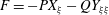
Since exact solutions are available for symmetric and antisymmetric waves, they can be used to check the accuracy of the numerical method. We have calculated the
 $L_{2}$
norm of the difference in the Fourier coefficients,
$L_{2}$
norm of the difference in the Fourier coefficients,
 $$\begin{eqnarray}\mathscr{L}=\left(\mathop{\sum }_{n=1}^{M}|a_{n}^{(e)}-a_{n}^{(c)}|^{2}\right)^{1/2},\end{eqnarray}$$
where
 $a_{n}^{(e)}$
,
$a_{n}^{(e)}$
,
 $a_{n}^{(c)}$
are the coefficients for the exact and numerically computed waves respectively and
$a_{n}^{(c)}$
are the coefficients for the exact and numerically computed waves respectively and
 $M<N$
is a chosen level of truncation (we note that in typical calculations, the level of machine precision is reached when
$M<N$
is a chosen level of truncation (we note that in typical calculations, the level of machine precision is reached when
 $N\approx 40$
at which point the Fourier coefficients are typically of size
$N\approx 40$
at which point the Fourier coefficients are typically of size
 $10^{-16}$
). By way of example, for a symmetric Kinnersley wave with
$10^{-16}$
). By way of example, for a symmetric Kinnersley wave with
 $H=3.0$
and
$H=3.0$
and
 $c=0.751$
we obtain
$c=0.751$
we obtain
 $\mathscr{L}=6.7\times 10^{-13}$
with
$\mathscr{L}=6.7\times 10^{-13}$
with
 $M=N=32$
and
$M=N=32$
and
 $\mathscr{L}=1.14\times 10^{-14}$
with
$\mathscr{L}=1.14\times 10^{-14}$
with
 $M=40$
,
$M=40$
,
 $N=128$
.
$N=128$
.
In the results to be presented below, we fix
 $H$
and vary
$H$
and vary
 $c$
from its value for a small-amplitude wave. In doing this, we trace a branch of travelling-wave solutions, eventually arriving at a limiting profile with a trapped bubble as
$c$
from its value for a small-amplitude wave. In doing this, we trace a branch of travelling-wave solutions, eventually arriving at a limiting profile with a trapped bubble as
 $c$
approaches a critical value. That this must happen is demonstrated in appendix C.
$c$
approaches a critical value. That this must happen is demonstrated in appendix C.
4 Linear stability
To study the linear stability of the travelling-wave solutions discussed in § 3, we introduce perturbations, writing
 $$\begin{eqnarray}x=X(\unicode[STIX]{x1D709})+\tilde{x}(\unicode[STIX]{x1D709},t),\quad y=Y(\unicode[STIX]{x1D709})+{\tilde{y}}(\unicode[STIX]{x1D709},t),\quad \unicode[STIX]{x1D719}=c\unicode[STIX]{x1D709}+\tilde{\unicode[STIX]{x1D719}}(\unicode[STIX]{x1D709},t),\quad \unicode[STIX]{x1D713}=\tilde{\unicode[STIX]{x1D713}}(\unicode[STIX]{x1D709},t),\quad\end{eqnarray}$$
and
 $$\begin{eqnarray}\hat{x}=\hat{X}(\unicode[STIX]{x1D709})+\tilde{\unicode[STIX]{x1D712}}(\unicode[STIX]{x1D709},t),\quad {\hat{y}}={\hat{Y}}(\unicode[STIX]{x1D709})+\tilde{b}(\unicode[STIX]{x1D709},t),\quad \hat{\unicode[STIX]{x1D719}}=c\unicode[STIX]{x1D709}+\tilde{\unicode[STIX]{x1D6F7}}(\unicode[STIX]{x1D709},t)\quad \hat{\unicode[STIX]{x1D713}}=\tilde{\unicode[STIX]{x1D6F9}}(\unicode[STIX]{x1D709},t),\quad\end{eqnarray}$$
where variables with a tilde are small. Note that it is not necessary to perturb the Bernoulli constant since any such perturbation can be absorbed into the perturbation for the velocity potential. We emphasise that the base waves are periodic with period
 $2\unicode[STIX]{x03C0}$
. Substituting (4.1) and (4.2) into the governing system (2.1)–(2.11) and linearising by neglecting products of the small perturbations, we obtain on the upper surface,
$2\unicode[STIX]{x03C0}$
. Substituting (4.1) and (4.2) into the governing system (2.1)–(2.11) and linearising by neglecting products of the small perturbations, we obtain on the upper surface,
 $$\begin{eqnarray}\displaystyle & {\tilde{y}}_{t}=Y_{\unicode[STIX]{x1D709}}[T(\tilde{\unicode[STIX]{x1D713}}_{\unicode[STIX]{x1D709}}/\text{J}_{0})-S(\tilde{\unicode[STIX]{x1D6F9}}_{\unicode[STIX]{x1D709}}/\hat{\text{J}}_{0})]-X_{\unicode[STIX]{x1D709}}\tilde{\unicode[STIX]{x1D713}}_{\unicode[STIX]{x1D709}}/\text{J}_{0},\qquad & \displaystyle\end{eqnarray}$$
 $$\begin{eqnarray}\displaystyle & \tilde{\unicode[STIX]{x1D719}}_{t}+c[S(\tilde{\unicode[STIX]{x1D6F9}}_{\unicode[STIX]{x1D709}}/\hat{\text{J}}_{0})-T(\tilde{\unicode[STIX]{x1D713}}_{\unicode[STIX]{x1D709}}/\text{J}_{0})]+c\tilde{\unicode[STIX]{x1D719}}_{\unicode[STIX]{x1D709}}/\text{J}_{0}+F\tilde{x}_{\unicode[STIX]{x1D709}}+G{\tilde{y}}_{\unicode[STIX]{x1D709}}+QY_{\unicode[STIX]{x1D709}}\tilde{x}_{\unicode[STIX]{x1D709}\unicode[STIX]{x1D709}}-QX_{\unicode[STIX]{x1D709}}{\tilde{y}}_{\unicode[STIX]{x1D709}\unicode[STIX]{x1D709}}=0,\qquad & \displaystyle\end{eqnarray}$$
 $$\begin{eqnarray}\displaystyle & \tilde{x}_{\unicode[STIX]{x1D709}}=S(\tilde{b}_{\unicode[STIX]{x1D709}})-T({\tilde{y}}_{\unicode[STIX]{x1D709}}),\quad \tilde{\unicode[STIX]{x1D719}}_{\unicode[STIX]{x1D709}}=S(\tilde{\unicode[STIX]{x1D6F9}}_{\unicode[STIX]{x1D709}})-T(\tilde{\unicode[STIX]{x1D713}}_{\unicode[STIX]{x1D709}}).\qquad & \displaystyle\end{eqnarray}$$
where
 $F=-PX_{\unicode[STIX]{x1D709}}-QY_{\unicode[STIX]{x1D709}\unicode[STIX]{x1D709}}$
,
$F=-PX_{\unicode[STIX]{x1D709}}-QY_{\unicode[STIX]{x1D709}\unicode[STIX]{x1D709}}$
,
 $G=-PY_{\unicode[STIX]{x1D709}}+QX_{\unicode[STIX]{x1D709}\unicode[STIX]{x1D709}}$
and
$G=-PY_{\unicode[STIX]{x1D709}}+QX_{\unicode[STIX]{x1D709}\unicode[STIX]{x1D709}}$
and
 $$\begin{eqnarray}P=(6\mathscr{B}\text{J}_{0}-c^{2})/(2\text{J}_{0}^{2}),\quad Q=1/\text{J}_{0}^{3/2}.\end{eqnarray}$$
On the lower surface we find
 $$\begin{eqnarray}\displaystyle & \tilde{b}_{t}={\hat{Y}}_{\unicode[STIX]{x1D709}}[S(\tilde{\unicode[STIX]{x1D713}}_{\unicode[STIX]{x1D709}}/\text{J}_{0})-T(\tilde{\unicode[STIX]{x1D6F9}}_{\unicode[STIX]{x1D709}}/\hat{\text{J}}_{0})]-\hat{X}_{\unicode[STIX]{x1D709}}\tilde{\unicode[STIX]{x1D6F9}}_{\unicode[STIX]{x1D709}}/\hat{\text{J}}_{0},\qquad \quad & \displaystyle\end{eqnarray}$$
 $$\begin{eqnarray}\displaystyle & \tilde{\unicode[STIX]{x1D6F7}}_{t}+c[T(\tilde{\unicode[STIX]{x1D6F9}}_{\unicode[STIX]{x1D709}}/\hat{\text{J}}_{0})-S(\tilde{\unicode[STIX]{x1D713}}_{\unicode[STIX]{x1D709}}/\text{J}_{0})]+c\tilde{\unicode[STIX]{x1D6F7}}_{\unicode[STIX]{x1D709}}/\hat{\text{J}}_{0}+\hat{F}\tilde{\unicode[STIX]{x1D712}}_{\unicode[STIX]{x1D709}}+{\hat{G}}\tilde{b}_{\unicode[STIX]{x1D709}}+\hat{Q}{\hat{Y}}_{\unicode[STIX]{x1D709}}\tilde{\unicode[STIX]{x1D712}}_{\unicode[STIX]{x1D709}\unicode[STIX]{x1D709}}-\hat{Q}\hat{X}_{\unicode[STIX]{x1D709}}\tilde{b}_{\unicode[STIX]{x1D709}\unicode[STIX]{x1D709}}=0,\qquad \quad & \displaystyle\end{eqnarray}$$
 $$\begin{eqnarray}\displaystyle & \tilde{\unicode[STIX]{x1D712}}_{\unicode[STIX]{x1D709}}=T(\tilde{b}_{\unicode[STIX]{x1D709}})-S({\tilde{y}}_{\unicode[STIX]{x1D709}}),\quad \tilde{\unicode[STIX]{x1D6F7}}_{\unicode[STIX]{x1D709}}=T(\tilde{\unicode[STIX]{x1D6F9}}_{\unicode[STIX]{x1D709}})-S(\tilde{\unicode[STIX]{x1D713}}_{\unicode[STIX]{x1D709}}),\qquad \quad & \displaystyle\end{eqnarray}$$
where
 $\hat{F}=-\hat{P}\hat{X}_{\unicode[STIX]{x1D709}}-\hat{Q}{\hat{Y}}_{\unicode[STIX]{x1D709}\unicode[STIX]{x1D709}}$
,
$\hat{F}=-\hat{P}\hat{X}_{\unicode[STIX]{x1D709}}-\hat{Q}{\hat{Y}}_{\unicode[STIX]{x1D709}\unicode[STIX]{x1D709}}$
,
 ${\hat{G}}=-\hat{P}{\hat{Y}}_{\unicode[STIX]{x1D709}}+\hat{Q}\hat{X}_{\unicode[STIX]{x1D709}\unicode[STIX]{x1D709}}$
and
${\hat{G}}=-\hat{P}{\hat{Y}}_{\unicode[STIX]{x1D709}}+\hat{Q}\hat{X}_{\unicode[STIX]{x1D709}\unicode[STIX]{x1D709}}$
and
 $$\begin{eqnarray}\hat{P}=(6\mathscr{B}\hat{\text{J}}_{0}-c^{2})/(2\hat{\text{J}}_{0}^{2}),\quad \hat{Q}=-1/\hat{\text{J}}_{0}^{3/2}.\end{eqnarray}$$
Invoking Floquet theory (see, for example, Sandstede Reference Sandstede and Fiedler2002), we express the perturbations in the form
 $$\begin{eqnarray}\left(\begin{array}{@{}c@{}}\tilde{x}\\ {\tilde{y}}\\ \tilde{\unicode[STIX]{x1D719}}\\ \tilde{\unicode[STIX]{x1D713}}\end{array}\right)=\text{e}^{\unicode[STIX]{x1D70E}t}\text{e}^{\text{i}p\unicode[STIX]{x1D709}}\mathop{\sum }_{n=-\infty }^{\infty }\boldsymbol{a}_{n}\text{e}^{\text{i}n\unicode[STIX]{x1D709}},\quad \left(\begin{array}{@{}c@{}}\tilde{\unicode[STIX]{x1D712}}\\ \tilde{b}\\ \tilde{\unicode[STIX]{x1D6F7}}\\ \tilde{\unicode[STIX]{x1D6F9}}\end{array}\right)=\text{e}^{\unicode[STIX]{x1D70E}t}\text{e}^{\text{i}p\unicode[STIX]{x1D709}}\mathop{\sum }_{n=-\infty }^{\infty }\hat{\boldsymbol{a}}_{n}\text{e}^{\text{i}n\unicode[STIX]{x1D709}},\end{eqnarray}$$
where the constant Fourier coefficients
 $\boldsymbol{a}_{n}=(a_{n},b_{n},c_{n},d_{n})^{\text{T}}$
and
$\boldsymbol{a}_{n}=(a_{n},b_{n},c_{n},d_{n})^{\text{T}}$
and
 $\hat{\boldsymbol{a}}_{n}=(\hat{a}_{n},\hat{b}_{n},{\hat{c}}_{n},\hat{d}_{n})^{\text{T}}$
and the generally complex growth rate
$\hat{\boldsymbol{a}}_{n}=(\hat{a}_{n},\hat{b}_{n},{\hat{c}}_{n},\hat{d}_{n})^{\text{T}}$
and the generally complex growth rate
 $\unicode[STIX]{x1D70E}=\unicode[STIX]{x1D70E}_{R}+\text{i}\unicode[STIX]{x1D70E}_{I}$
are to be found. If
$\unicode[STIX]{x1D70E}=\unicode[STIX]{x1D70E}_{R}+\text{i}\unicode[STIX]{x1D70E}_{I}$
are to be found. If
 $\unicode[STIX]{x1D70E}_{R}>0$
the flow is spectrally unstable and hence linearly unstable. The real parameter
$\unicode[STIX]{x1D70E}_{R}>0$
the flow is spectrally unstable and hence linearly unstable. The real parameter
 $p$
is prescribed. When
$p$
is prescribed. When
 $p=0$
, or any integer, the perturbation has the same wavelength as the steady base wave and the mode is termed superharmonic. For
$p=0$
, or any integer, the perturbation has the same wavelength as the steady base wave and the mode is termed superharmonic. For
 $p$
not an integer, the perturbation is termed subharmonic and contains modes of wavelength longer than the steady wave. If
$p$
not an integer, the perturbation is termed subharmonic and contains modes of wavelength longer than the steady wave. If
 $p$
is irrational the perturbation is subharmonic but quasiperiodic and as such cannot be captured by the present formulation which assumes periodicity. Following Chen & Saffman (Reference Chen and Saffman1985), we may restrict
$p$
is irrational the perturbation is subharmonic but quasiperiodic and as such cannot be captured by the present formulation which assumes periodicity. Following Chen & Saffman (Reference Chen and Saffman1985), we may restrict
 $p$
to the range
$p$
to the range
 $[0,1)$
without loss of generality.
$[0,1)$
without loss of generality.
We substitute (4.11) into (4.5) and (4.9) and derive the following relations valid when
 $n+p\neq 0$
,
$n+p\neq 0$
,
 $$\begin{eqnarray}\displaystyle & a_{n}=\text{i}\hat{b}_{n}\,\text{cosech}([n+p]H)-\text{i}b_{n}\,\text{coth}([n+p]H), & \displaystyle\end{eqnarray}$$
 $$\begin{eqnarray}\displaystyle & d_{n}=\text{i}c_{n}\,\text{coth}([n+p]H)-\text{i}{\hat{c}}_{n}\,\text{cosech}([n+p]H), & \displaystyle\end{eqnarray}$$
 $$\begin{eqnarray}\displaystyle & \hat{a}_{n}=\text{i}\hat{b}_{n}\,\text{coth}([n+p]H)-\text{i}b_{n}\,\text{cosech}([n+p]H), & \displaystyle\end{eqnarray}$$
 $$\begin{eqnarray}\displaystyle & \hat{d}_{n}=\text{i}c_{n}\,\text{cosech}([n+p]H)-\text{i}{\hat{c}}_{n}\,\text{coth}([n+p]H), & \displaystyle\end{eqnarray}$$
which we may use to eliminate
 $a_{j}$
,
$a_{j}$
,
 $d_{j}$
,
$d_{j}$
,
 $\hat{a}_{j}$
,
$\hat{a}_{j}$
,
 $\hat{d}_{j}$
. To prepare the system for numerical computation, we truncate the infinite series in (4.11) at the
$\hat{d}_{j}$
. To prepare the system for numerical computation, we truncate the infinite series in (4.11) at the
 $N$
th harmonic by setting
$N$
th harmonic by setting
 $\boldsymbol{a}_{n}=\hat{\boldsymbol{a}}_{n}=\mathbf{0}$
for
$\boldsymbol{a}_{n}=\hat{\boldsymbol{a}}_{n}=\mathbf{0}$
for
 $|n|>N$
. Substituting the truncated forms of (4.11) into the remaining equations in (4.3)–(4.10) evaluated at the collocation points (3.8), we compile the matrix system
$|n|>N$
. Substituting the truncated forms of (4.11) into the remaining equations in (4.3)–(4.10) evaluated at the collocation points (3.8), we compile the matrix system
 $$\begin{eqnarray}\unicode[STIX]{x1D70E}\unicode[STIX]{x1D647}\boldsymbol{x}=\unicode[STIX]{x1D64D}\boldsymbol{x},\end{eqnarray}$$
where
 $\boldsymbol{x}=(b_{-N},\ldots ,b_{N},c_{-N},\ldots ,c_{N},\hat{b}_{-N},\ldots ,\hat{b}_{N},{\hat{c}}_{-N},\ldots ,{\hat{c}}_{N})^{\text{T}}$
, and
$\boldsymbol{x}=(b_{-N},\ldots ,b_{N},c_{-N},\ldots ,c_{N},\hat{b}_{-N},\ldots ,\hat{b}_{N},{\hat{c}}_{-N},\ldots ,{\hat{c}}_{N})^{\text{T}}$
, and
 $\unicode[STIX]{x1D647}$
and
$\unicode[STIX]{x1D647}$
and
 $\unicode[STIX]{x1D64D}$
are
$\unicode[STIX]{x1D64D}$
are
 $(8N+4)\times (8N+4)$
matrices given by
$(8N+4)\times (8N+4)$
matrices given by
 $$\begin{eqnarray}\unicode[STIX]{x1D647}=\left(\begin{array}{@{}cccc@{}}\boldsymbol{E} & \mathbf{0} & \mathbf{0} & \mathbf{0}\\ \boldsymbol{ 0} & \boldsymbol{E} & \mathbf{0} & \mathbf{0}\\ \boldsymbol{ 0} & \mathbf{0} & \boldsymbol{E} & \mathbf{0}\\ \boldsymbol{ 0} & \mathbf{0} & \mathbf{0} & \boldsymbol{E}\end{array}\right),\quad \unicode[STIX]{x1D64D}=\left(\begin{array}{@{}cccc@{}}\mathbf{0} & \boldsymbol{A} & \mathbf{0} & \hat{\boldsymbol{A}}\\ \boldsymbol{B} & c\boldsymbol{G} & \hat{\boldsymbol{B}} & c\hat{\boldsymbol{G}}\\ \boldsymbol{ 0} & \unicode[STIX]{x1D734} & \mathbf{0} & \hat{\unicode[STIX]{x1D734}}\\ \unicode[STIX]{x1D71F} & c\boldsymbol{M} & \hat{\unicode[STIX]{x1D71F}} & c\hat{\boldsymbol{M}}\end{array}\right),\end{eqnarray}$$
and where all of the submatrices are of size
 $(2N+1)\times (2N+1)$
. Here
$(2N+1)\times (2N+1)$
. Here
 $\boldsymbol{E}_{k,l}=\exp \{\text{i}(l^{\prime }+p)\unicode[STIX]{x1D709}_{k}\}$
and
$\boldsymbol{E}_{k,l}=\exp \{\text{i}(l^{\prime }+p)\unicode[STIX]{x1D709}_{k}\}$
and
 $$\begin{eqnarray}\left.\begin{array}{@{}c@{}}\displaystyle \boldsymbol{A}_{k,l}=(l^{\prime }+p)\left[\frac{X_{\unicode[STIX]{x1D709}}}{\text{J}_{0}}q_{1}\boldsymbol{E}_{k,l}+Y_{\unicode[STIX]{x1D709}}(q_{2}\hat{\unicode[STIX]{x1D707}}_{k,l}-q_{1}\unicode[STIX]{x1D708}_{k,l})\right],\\ \displaystyle \boldsymbol{B}_{k,l}=-(l^{\prime }+p)[q_{1}(F+\text{i}(l^{\prime }+p)QY_{\unicode[STIX]{x1D709}})+G\text{i}+QX_{\unicode[STIX]{x1D709}}(l^{\prime }+p)]\boldsymbol{E}_{k,l},\\ \displaystyle \boldsymbol{G}_{k,l}=-(l^{\prime }+p)\left[\frac{\text{i}}{\text{J}_{0}}\boldsymbol{E}_{k,l}+(q_{1}\unicode[STIX]{x1D708}_{k,l}-q_{2}\hat{\unicode[STIX]{x1D707}}_{k,l})\right],\\ \displaystyle \unicode[STIX]{x1D734}_{k,l}=(l^{\prime }+p)\left[\frac{\hat{X}_{\unicode[STIX]{x1D709}}}{\hat{\text{J}}_{0}}q_{2}\boldsymbol{E}_{k,l}+{\hat{Y}}_{\unicode[STIX]{x1D709}}(q_{2}\hat{\unicode[STIX]{x1D708}}_{k,l}-q_{1}\unicode[STIX]{x1D707}_{k,l})\right],\\ \unicode[STIX]{x1D71F}_{k,l}=-(l^{\prime }+p)q_{2}[\hat{F}+\text{i}(l^{\prime }+p)\hat{Q}{\hat{Y}}_{\unicode[STIX]{x1D709}}]\boldsymbol{E}_{k,l},\\ \boldsymbol{M}_{k,l}=(l^{\prime }+p)(q_{2}\hat{\unicode[STIX]{x1D708}}_{k,l}-q_{1}\unicode[STIX]{x1D707}_{k,l})\end{array}\right\}\end{eqnarray}$$
and
 $$\begin{eqnarray}\left.\begin{array}{@{}c@{}}\displaystyle \hat{\boldsymbol{A}}_{k,l}=(l^{\prime }+p)\left[-\frac{X_{\unicode[STIX]{x1D709}}}{\text{J}_{0}}q_{2}\boldsymbol{E}_{k,l}+Y_{\unicode[STIX]{x1D709}}(q_{2}\unicode[STIX]{x1D708}_{k,l}-q_{1}\hat{\unicode[STIX]{x1D707}}_{k,l})\right],\\ \hat{\boldsymbol{B}}_{k,l}=(l^{\prime }+p)q_{2}[F+\text{i}(l^{\prime }+p)QY_{\unicode[STIX]{x1D709}}]\boldsymbol{E}_{k,l},\\ \hat{\boldsymbol{G}}_{k,l}=(l^{\prime }+p)(q_{2}\unicode[STIX]{x1D708}_{k,l}-q_{1}\hat{\unicode[STIX]{x1D707}}_{k,l}),\\ \displaystyle \hat{\unicode[STIX]{x1D734}}_{k,l}=(l^{\prime }+p)\left[-\frac{\hat{X}_{\unicode[STIX]{x1D709}}}{\hat{\text{J}}_{0}}q_{1}\boldsymbol{E}_{k,l}+{\hat{Y}}_{\unicode[STIX]{x1D709}}(q_{2}\unicode[STIX]{x1D707}_{k,l}-q_{1}\hat{\unicode[STIX]{x1D708}}_{k,l})\right],\\ \hat{\unicode[STIX]{x1D71F}}_{k,l}=(l^{\prime }+p)[q_{1}(\hat{F}+\text{i}(l^{\prime }+p)\hat{Q}{\hat{Y}}_{\unicode[STIX]{x1D709}})-{\hat{G}}\text{i}-\hat{Q}\hat{X}_{\unicode[STIX]{x1D709}}(l^{\prime }+p)]\boldsymbol{E}_{k,l},\\ \displaystyle \hat{\boldsymbol{M}}_{k,l}=-(l^{\prime }+p)\left[\frac{\text{i}}{\hat{\text{J}}_{0}}\boldsymbol{E}_{k,l}+(q_{1}\hat{\unicode[STIX]{x1D708}}_{k,l}-q_{2}\unicode[STIX]{x1D707}_{k,l})\right],\end{array}\right\}\end{eqnarray}$$
where
 $l^{\prime }=l-(N+1)$
, and
$l^{\prime }=l-(N+1)$
, and
 $q_{1}=\text{coth}([l^{\prime }+p]H)$
and
$q_{1}=\text{coth}([l^{\prime }+p]H)$
and
 $q_{2}=\text{cosech}([l^{\prime }+p]H)$
. All of the terms in the matrix elements are evaluated at the collocation points
$q_{2}=\text{cosech}([l^{\prime }+p]H)$
. All of the terms in the matrix elements are evaluated at the collocation points
 $\unicode[STIX]{x1D709}=\unicode[STIX]{x1D709}_{k}$
. Also,
$\unicode[STIX]{x1D709}=\unicode[STIX]{x1D709}_{k}$
. Also,
 $$\begin{eqnarray}\displaystyle & \displaystyle \unicode[STIX]{x1D707}_{k,l}=\text{i}\mathop{\sum }_{j=-N}^{N}u_{j}\,\text{cosech}([j+l^{\prime }+p]H)\text{e}^{\text{i}(j+l^{\prime }+p)\unicode[STIX]{x1D709}_{k}}, & \displaystyle\end{eqnarray}$$
 $$\begin{eqnarray}\displaystyle & \displaystyle \unicode[STIX]{x1D708}_{k,l}=\text{i}\mathop{\sum }_{j=-N}^{N}u_{j}\,\text{coth}([j+l^{\prime }+p]H)\text{e}^{\text{i}(j+l^{\prime }+p)\unicode[STIX]{x1D709}_{k}}, & \displaystyle\end{eqnarray}$$
 $$\begin{eqnarray}\displaystyle & \displaystyle \hat{\unicode[STIX]{x1D707}}_{k,l}=\text{i}\mathop{\sum }_{j=-N}^{N}\hat{u} _{j}\,\text{cosech}([j+l^{\prime }+p]H)\text{e}^{\text{i}(j+l^{\prime }+p)\unicode[STIX]{x1D709}_{k}}, & \displaystyle\end{eqnarray}$$
 $$\begin{eqnarray}\displaystyle & \displaystyle \hat{\unicode[STIX]{x1D708}}_{k,l}=\text{i}\mathop{\sum }_{j=-N}^{N}\hat{u} _{j}\,\text{cosech}([j+l^{\prime }+p]H)\text{e}^{\text{i}(j+l^{\prime }+p)\unicode[STIX]{x1D709}_{k}}, & \displaystyle\end{eqnarray}$$
where
 $u_{j}$
and
$u_{j}$
and
 $\hat{u} _{j}$
are the coefficients in the Fourier expansion of
$\hat{u} _{j}$
are the coefficients in the Fourier expansion of
 $1/\text{J}_{0}$
and
$1/\text{J}_{0}$
and
 $1/\hat{\text{J}}_{0}$
respectively. The expressions (4.20)–(4.23) originate in the non-local terms in (4.3), (4.4), (4.7) and (4.8). To obtain these we have used the facts that for
$1/\hat{\text{J}}_{0}$
respectively. The expressions (4.20)–(4.23) originate in the non-local terms in (4.3), (4.4), (4.7) and (4.8). To obtain these we have used the facts that for
 $n\neq 0$
 $$\begin{eqnarray}T(\text{e}^{\text{i}n\unicode[STIX]{x1D709}})=\text{i}\,\text{coth}(nH)\text{e}^{\text{i}n\unicode[STIX]{x1D709}},\quad S(\text{e}^{\text{i}n\unicode[STIX]{x1D709}})=\text{i}\,\text{cosech}(nH)\text{e}^{\text{i}n\unicode[STIX]{x1D709}}.\end{eqnarray}$$
We note that when
 $(l^{\prime }+p)=0$
in (4.18)–(4.19), we set
$(l^{\prime }+p)=0$
in (4.18)–(4.19), we set
 $(l^{\prime }+p)\text{coth}([l^{\prime }+p]H)=0$
and
$(l^{\prime }+p)\text{coth}([l^{\prime }+p]H)=0$
and
 $(l^{\prime }+p)\text{cosech}([l^{\prime }+p]H)=0$
. For the sums in (4.20)–(4.23), when
$(l^{\prime }+p)\text{cosech}([l^{\prime }+p]H)=0$
. For the sums in (4.20)–(4.23), when
 $j+l^{\prime }+p=0$
we set the corresponding term in each sum to zero in accordance with the principal value definition of the operators (2.7) and (2.8).
$j+l^{\prime }+p=0$
we set the corresponding term in each sum to zero in accordance with the principal value definition of the operators (2.7) and (2.8).
The eigenspectrum has the property that if (i)
 $\{\unicode[STIX]{x1D70E},p,b_{j},c_{j},\hat{b}_{j},{\hat{c}}_{j}\}$
is an eigenset then so are
$\{\unicode[STIX]{x1D70E},p,b_{j},c_{j},\hat{b}_{j},{\hat{c}}_{j}\}$
is an eigenset then so are
 $$\begin{eqnarray}\left.\begin{array}{@{}c@{}}\text{(ii)}~\{\unicode[STIX]{x1D70E}^{\ast },-p,b_{-j}^{\ast },c_{-j}^{\ast },\hat{b}_{-j}^{\ast },{\hat{c}}_{-j}^{\ast }\},\quad \text{(iii)}~\{-\unicode[STIX]{x1D70E},-p,b_{-j},-c_{-j},\hat{b}_{-j},-{\hat{c}}_{-j}\},\\ \text{(iv)}~\{-\unicode[STIX]{x1D70E}^{\ast },p,b_{j}^{\ast },-c_{j}^{\ast },\hat{b}_{j}^{\ast },-{\hat{c}}_{j}^{\ast }\}.\end{array}\right\}\end{eqnarray}$$
These can be shown using arguments similar to those presented by Tiron & Choi (Reference Tiron and Choi2012) for the case of infinite depth. Given the aforementioned symmetry properties, we may further restrict the range of
 $p$
for the stability problem to
$p$
for the stability problem to
 $p\in [0,1/2]$
(see also Tiron & Choi Reference Tiron and Choi2012).
$p\in [0,1/2]$
(see also Tiron & Choi Reference Tiron and Choi2012).
When both the upper and the lower surface is flat, Taylor (Reference Taylor1959) showed that two types of small-amplitude perturbation are possible: symmetric waves with troughs on the upper wave facing crests on the lower wave and antisymmetric waves with troughs on the upper wave opposing troughs on the lower waves (see also Squire Reference Squire1953). Taylor showed that the symmetric waves of period
 $2\unicode[STIX]{x03C0}$
travel at speed
$2\unicode[STIX]{x03C0}$
travel at speed
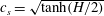 $c_{s}=\sqrt{\tanh (H/2)}$
and the antisymmetric waves travel at speed
$c_{s}=\sqrt{\tanh (H/2)}$
and the antisymmetric waves travel at speed
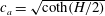 $c_{a}=\sqrt{\text{coth}(H/2)}$
. As noted above, we are presently working in a frame of reference travelling with the speed of the basic periodic wave whose stability we wish to study. We find that for perturbations about the flat state,
$c_{a}=\sqrt{\text{coth}(H/2)}$
. As noted above, we are presently working in a frame of reference travelling with the speed of the basic periodic wave whose stability we wish to study. We find that for perturbations about the flat state,
 $\unicode[STIX]{x1D70E}=\unicode[STIX]{x1D70E}_{s,m}^{\unicode[STIX]{x1D708}}$
or
$\unicode[STIX]{x1D70E}=\unicode[STIX]{x1D70E}_{s,m}^{\unicode[STIX]{x1D708}}$
or
 $\unicode[STIX]{x1D70E}_{a,m}^{\unicode[STIX]{x1D708}}$
, where
$\unicode[STIX]{x1D70E}_{a,m}^{\unicode[STIX]{x1D708}}$
, where
 $$\begin{eqnarray}\displaystyle & \displaystyle \unicode[STIX]{x1D70E}_{s,m}^{\unicode[STIX]{x1D708}}=\text{i}\unicode[STIX]{x1D708}[p^{\prime 3}\tanh (p^{\prime }H/2)]^{1/2}-\text{i}p^{\prime }c_{f}, & \displaystyle\end{eqnarray}$$
 $$\begin{eqnarray}\displaystyle & \displaystyle \unicode[STIX]{x1D70E}_{a,m}^{\unicode[STIX]{x1D708}}=\text{i}\unicode[STIX]{x1D708}[p^{\prime 3}\,\text{coth}(p^{\prime }H/2)]^{1/2}-\text{i}p^{\prime }c_{f}, & \displaystyle\end{eqnarray}$$
where
 $\unicode[STIX]{x1D708}=\pm 1$
, and
$\unicode[STIX]{x1D708}=\pm 1$
, and
 $p^{\prime }=p+m$
for any integer
$p^{\prime }=p+m$
for any integer
 $m$
and
$m$
and
 $c_{f}=c_{s}$
or
$c_{f}=c_{s}$
or
 $c_{a}$
. Since
$c_{a}$
. Since
 $p\in [0,1/2]$
and we have the symmetries in (4.25), it follows that
$p\in [0,1/2]$
and we have the symmetries in (4.25), it follows that
 $p^{\prime }$
covers the whole real line. Hence formulae (4.26), (4.27) cover all possible symmetric and antisymmetric waves with wavenumber
$p^{\prime }$
covers the whole real line. Hence formulae (4.26), (4.27) cover all possible symmetric and antisymmetric waves with wavenumber
 $p^{\prime }$
written relative to the speed of a symmetric or antisymmetric wave of unit wavenumber. It should be noted that both of the growth rates in (4.26), (4.27) are purely imaginary, corresponding to neutral travelling waves.
$p^{\prime }$
written relative to the speed of a symmetric or antisymmetric wave of unit wavenumber. It should be noted that both of the growth rates in (4.26), (4.27) are purely imaginary, corresponding to neutral travelling waves.
The generalised eigenvalue problem (4.16) was solved numerically using the inbuilt MATLAB function eig. The level of truncation
 $N$
was varied according to the base wave under scrutiny to ensure accuracy of the computation. An accuracy check is carried out in § 5. We note that we have verified our numerical results by successfully comparing against independent calculations performed by Dr Z. Wang (2015, private communication).
$N$
was varied according to the base wave under scrutiny to ensure accuracy of the computation. An accuracy check is carried out in § 5. We note that we have verified our numerical results by successfully comparing against independent calculations performed by Dr Z. Wang (2015, private communication).
4.1 Time-dependent numerical method
In addition to solving the eigenvalue problem for the growth rates discussed in § 4, we have also solved the unsteady equations (2.1)–(2.4) numerically using a pseudospectral scheme. The unknown variables are represented as Fourier expansions and the spatial derivatives are computed spectrally in Fourier space. The nonlinear terms are computed in real space and the solution is marched forward in time using the fourth-order Runge–Kutta method. To handle the non-local operators, we use the fact that if
 $$\begin{eqnarray}\hat{f}(k)=\mathscr{F}[f(\unicode[STIX]{x1D709})]=\int _{-\infty }^{\infty }f(\unicode[STIX]{x1D709})\text{e}^{-\text{i}k\unicode[STIX]{x1D709}}\,\text{d}\unicode[STIX]{x1D709}\end{eqnarray}$$
then
 $$\begin{eqnarray}\left.\begin{array}{@{}c@{}}T(f_{\unicode[STIX]{x1D709}}(\unicode[STIX]{x1D709}))=-\mathscr{F}^{-1}(k\,\text{coth}(kH)\hat{f}),\quad S(f_{\unicode[STIX]{x1D709}}(\unicode[STIX]{x1D709}))=-\mathscr{F}^{-1}(k\,\text{cosech}(kH)\hat{f})\quad (k\neq 0),\\ T(f_{\unicode[STIX]{x1D709}}(\unicode[STIX]{x1D709}))=S(f_{\unicode[STIX]{x1D709}}(\unicode[STIX]{x1D709}))=0\quad (k=0).\end{array}\right\}\end{eqnarray}$$
5 Results
The solution space for steady waves is parametrised by
 $H$
and
$H$
and
 $c$
. In what follows, we always fix
$c$
. In what follows, we always fix
 $H$
and vary
$H$
and vary
 $c$
to delineate the branch of steady wave profiles and determine their stability. We have checked that for a large value of
$c$
to delineate the branch of steady wave profiles and determine their stability. We have checked that for a large value of
 $H$
we recover the results of the stability calculations of Tiron & Choi (Reference Tiron and Choi2012) for the infinite depth case. For a fixed finite value of
$H$
we recover the results of the stability calculations of Tiron & Choi (Reference Tiron and Choi2012) for the infinite depth case. For a fixed finite value of
 $H$
, symmetric waves bifurcate from
$H$
, symmetric waves bifurcate from
 $c=c_{s}$
and antisymmetric waves bifurcate from
$c=c_{s}$
and antisymmetric waves bifurcate from
 $c=c_{a}$
. In each case, there is a finite range of
$c=c_{a}$
. In each case, there is a finite range of
 $c$
values over which physically meaningful, that is not self-intersecting, steady wave profiles are possible (see appendix C). At the limit of this range the nonlinear wave profiles always exhibit a trapped air bubble.
$c$
values over which physically meaningful, that is not self-intersecting, steady wave profiles are possible (see appendix C). At the limit of this range the nonlinear wave profiles always exhibit a trapped air bubble.

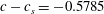
Figure 1. Steady symmetric waves (two periods are shown): (a,c)
 $H=1$
and (b,d)
$H=1$
and (b,d)
 $H=4$
; (a,b)
$H=4$
; (a,b)
 $c-c_{s}=-0.35$
and
$c-c_{s}=-0.35$
and
 $-$
0.1 respectively; and (c,d)
$-$
0.1 respectively; and (c,d)
 $c-c_{s}=-0.5785$
and
$c-c_{s}=-0.5785$
and
 $-$
0.22 respectively. The insets show close-ups near to the high curvature regions. Note that in the (c,d) inset the upper/lower waves are very close together but are not actually in contact. The waves have been translated upwards for display purposes.
$-$
0.22 respectively. The insets show close-ups near to the high curvature regions. Note that in the (c,d) inset the upper/lower waves are very close together but are not actually in contact. The waves have been translated upwards for display purposes.
5.1 Superharmonic perturbations,
 $p=0$
$p=0$

We begin with a discussion of superharmonic perturbations to symmetric waves. Some steady wave profiles are shown in figure 1 for
 $H=1$
and
$H=1$
and
 $H=4$
for sample values of the wave speed
$H=4$
for sample values of the wave speed
 $c-c_{s}$
. These waves were computed numerically using the method described in § 3. In both cases the limiting profiles, obtained as the deviation from the linear wave speed
$c-c_{s}$
. These waves were computed numerically using the method described in § 3. In both cases the limiting profiles, obtained as the deviation from the linear wave speed
 $|c-c_{s}|$
increases, have trapped bubbles. The results of the stability calculations for the case
$|c-c_{s}|$
increases, have trapped bubbles. The results of the stability calculations for the case
 $H=1$
are shown in figure 2. At
$H=1$
are shown in figure 2. At
 $c\approx c_{s}$
the amplitude of the waves is small and the eigenvalues are all purely imaginary, so that the real part of the growth rate
$c\approx c_{s}$
the amplitude of the waves is small and the eigenvalues are all purely imaginary, so that the real part of the growth rate
 $\unicode[STIX]{x1D70E}_{R}$
is zero for the whole spectrum. The imaginary part of the eigenvalue spectrum,
$\unicode[STIX]{x1D70E}_{R}$
is zero for the whole spectrum. The imaginary part of the eigenvalue spectrum,
 $\unicode[STIX]{x1D70E}_{I}$
, is plotted against
$\unicode[STIX]{x1D70E}_{I}$
, is plotted against
 $c-c_{s}$
in figure 2(a) up to
$c-c_{s}$
in figure 2(a) up to
 $c-c_{s}=-0.55$
. As
$c-c_{s}=-0.55$
. As
 $c-c_{s}\rightarrow 0$
, the eigenvalues connect to the theoretical predictions of linear theory (4.26) and (4.27). The real part of the spectrum is shown in figure 2(b). Bubbles of instability appear following the coalescence of pairs of imaginary eigenvalues. Specifically each bubble emerges as two pairs of imaginary eigenvalues collide (in the upper half-plane and their reflection in the lower half plane) and move out into the complex plane to form a quartet of complex eigenvalues containing two conjugate pairs fulfilling the symmetries (4.25), two eigenvalues of which are unstable. Two instability bubbles are found over the range shown and these are labelled
$c-c_{s}\rightarrow 0$
, the eigenvalues connect to the theoretical predictions of linear theory (4.26) and (4.27). The real part of the spectrum is shown in figure 2(b). Bubbles of instability appear following the coalescence of pairs of imaginary eigenvalues. Specifically each bubble emerges as two pairs of imaginary eigenvalues collide (in the upper half-plane and their reflection in the lower half plane) and move out into the complex plane to form a quartet of complex eigenvalues containing two conjugate pairs fulfilling the symmetries (4.25), two eigenvalues of which are unstable. Two instability bubbles are found over the range shown and these are labelled
 $A$
and
$A$
and
 $B$
in the figures. In both panels (a) and (b), we have restricted the range of the imaginary part to
$B$
in the figures. In both panels (a) and (b), we have restricted the range of the imaginary part to
 $0<\unicode[STIX]{x1D70E}_{I}<15$
, but further computations reveal that more collisions occur beyond this range. The eigenspectrum at
$0<\unicode[STIX]{x1D70E}_{I}<15$
, but further computations reveal that more collisions occur beyond this range. The eigenspectrum at
 $c-c_{s}=-0.35$
is shown in figure 3. We note that a large number of Fourier modes are required to accurately capture the spectrum over the range shown. The figure indicates that for this value of
$c-c_{s}=-0.35$
is shown in figure 3. We note that a large number of Fourier modes are required to accurately capture the spectrum over the range shown. The figure indicates that for this value of
 $c-c_{s}$
, the most unstable mode has growth rate
$c-c_{s}$
, the most unstable mode has growth rate
 $\unicode[STIX]{x1D70E}=0.357+26.9\text{i}$
. Of course it may be the case that an eigenvalue with imaginary part off the scale shown in the figure has a larger real part than this value. We note that the cluster of 16 eigenvalues toward the bottom of the figure lie on an ellipse (a best-fit ellipse is superimposed in the figure).
$\unicode[STIX]{x1D70E}=0.357+26.9\text{i}$
. Of course it may be the case that an eigenvalue with imaginary part off the scale shown in the figure has a larger real part than this value. We note that the cluster of 16 eigenvalues toward the bottom of the figure lie on an ellipse (a best-fit ellipse is superimposed in the figure).

Figure 2. Eigenvalues for symmetric waves with
 $H=1$
: (a) Imaginary part,
$H=1$
: (a) Imaginary part,
 $\unicode[STIX]{x1D70E}_{I}$
and (b) real part
$\unicode[STIX]{x1D70E}_{I}$
and (b) real part
 $\unicode[STIX]{x1D70E}_{R}$
versus relative wave speed
$\unicode[STIX]{x1D70E}_{R}$
versus relative wave speed
 $c-c_{s}$
for superharmonic disturbances,
$c-c_{s}$
for superharmonic disturbances,
 $p=0$
. Bubbles of instability are labelled
$p=0$
. Bubbles of instability are labelled
 $A$
and
$A$
and
 $B$
.
$B$
.
Table 1. Accuracy check for the unstable eigenvalue on loop A, here labelled
 $\unicode[STIX]{x1D70E}^{(A)}$
, at
$\unicode[STIX]{x1D70E}^{(A)}$
, at
 $c-c_{s}=-0.35$
in figure 2. The tolerance for the Newton iterations for the base-wave calculation (see § 3) is
$c-c_{s}=-0.35$
in figure 2. The tolerance for the Newton iterations for the base-wave calculation (see § 3) is
 $\unicode[STIX]{x1D6FF}=10^{-11}$
.
$\unicode[STIX]{x1D6FF}=10^{-11}$
.

The calculations presented in figure 2 were carried out with
 $N=128$
. In table 1 we demonstrate the numerical convergence of the eigenvalue on bubble A in figure 2 at
$N=128$
. In table 1 we demonstrate the numerical convergence of the eigenvalue on bubble A in figure 2 at
 $c-c_{s}=-0.35$
as
$c-c_{s}=-0.35$
as
 $N$
is increased. Evidently the unstable eigenvalue is computed to a high degree of accuracy. To further validate the result, we compare the growth rate of a sample eigenmode from the spectrum found at
$N$
is increased. Evidently the unstable eigenvalue is computed to a high degree of accuracy. To further validate the result, we compare the growth rate of a sample eigenmode from the spectrum found at
 $c-c_{s}=-0.35$
with the results of a time-dependent simulation. We select the mode with complex growth rate
$c-c_{s}=-0.35$
with the results of a time-dependent simulation. We select the mode with complex growth rate
 $\unicode[STIX]{x1D70E}=0.1758+13.45\text{i}$
and solve the unsteady equations (2.1)–(2.4) as described in § 4.1. We track the time evolution of a small perturbation from the base wave with the initial condition
$\unicode[STIX]{x1D70E}=0.1758+13.45\text{i}$
and solve the unsteady equations (2.1)–(2.4) as described in § 4.1. We track the time evolution of a small perturbation from the base wave with the initial condition
 $$\begin{eqnarray}y(\unicode[STIX]{x1D709},0)=Y(\unicode[STIX]{x1D709})+{\tilde{y}}(\unicode[STIX]{x1D709},0),\quad {\tilde{y}}(\unicode[STIX]{x1D709},0)=\unicode[STIX]{x1D716}\left[\mathop{\sum }_{n=-N}^{N}{\tilde{y}}_{1n}\text{e}^{\text{i}n\unicode[STIX]{x1D709}}+\mathop{\sum }_{n=-N}^{N}{\tilde{y}}_{2n}\text{e}^{\text{i}n\unicode[STIX]{x1D709}}\right],\end{eqnarray}$$
where the coefficients
 ${\tilde{y}}_{1n}$
and
${\tilde{y}}_{1n}$
and
 ${\tilde{y}}_{2n}$
correspond to the eigenfunctions associated with
${\tilde{y}}_{2n}$
correspond to the eigenfunctions associated with
 $\unicode[STIX]{x1D70E}$
and
$\unicode[STIX]{x1D70E}$
and
 $\unicode[STIX]{x1D70E}^{\ast }$
respectively, and we choose
$\unicode[STIX]{x1D70E}^{\ast }$
respectively, and we choose
 $\unicode[STIX]{x1D716}=10^{-4}$
to facilitate comparison with linear theory. The symmetry properties of the eigensets (4.25) for
$\unicode[STIX]{x1D716}=10^{-4}$
to facilitate comparison with linear theory. The symmetry properties of the eigensets (4.25) for
 $p=0$
guarantee that
$p=0$
guarantee that
 $y(\unicode[STIX]{x1D709},0)$
in (5.1) is real. Analogous initial conditions are imposed for
$y(\unicode[STIX]{x1D709},0)$
in (5.1) is real. Analogous initial conditions are imposed for
 $b$
,
$b$
,
 $\unicode[STIX]{x1D719}$
and
$\unicode[STIX]{x1D719}$
and
 $\hat{\unicode[STIX]{x1D719}}$
. Consistent with the eigenvalue calculation, we fix the Bernoulli constant
$\hat{\unicode[STIX]{x1D719}}$
. Consistent with the eigenvalue calculation, we fix the Bernoulli constant
 $\mathscr{B}(t)$
during the time integration at the value corresponding to the steady wave solution. The perturbation
$\mathscr{B}(t)$
during the time integration at the value corresponding to the steady wave solution. The perturbation
 ${\tilde{y}}$
is shown in figure 4(a) at time
${\tilde{y}}$
is shown in figure 4(a) at time
 $t=2.0$
(note that in this case
$t=2.0$
(note that in this case
 $\tilde{b}=-{\tilde{y}}$
) and is seen to closely resemble the prediction of linear theory. Figure 4(b) shows the time evolution of the logarithm of the perturbation wave height,
$\tilde{b}=-{\tilde{y}}$
) and is seen to closely resemble the prediction of linear theory. Figure 4(b) shows the time evolution of the logarithm of the perturbation wave height,
 $L=\log (\max ({\tilde{y}})-\min ({\tilde{y}}))$
. This oscillates while growing at an exponential rate which convincingly matches the prediction of linear theory (shown with a broken line in the figure).
$L=\log (\max ({\tilde{y}})-\min ({\tilde{y}}))$
. This oscillates while growing at an exponential rate which convincingly matches the prediction of linear theory (shown with a broken line in the figure).

Figure 3. The eigenvalue spectrum for superharmonic disturbances (
 $p=0$
) for symmetric waves with
$p=0$
) for symmetric waves with
 $H=1$
at
$H=1$
at
 $c-c_{s}=-0.35$
. The solid lines are best-fit ellipses. The spectrum was computed using
$c-c_{s}=-0.35$
. The solid lines are best-fit ellipses. The spectrum was computed using
 $N=512$
. The label
$N=512$
. The label
 $A$
indicates the eigenvalue lying on loop
$A$
indicates the eigenvalue lying on loop
 $A$
in figure 2. Eigenvalues in the lower half are the reflection of those in the upper half-plane.
$A$
in figure 2. Eigenvalues in the lower half are the reflection of those in the upper half-plane.

Figure 4. Symmetric case for
 $H=1$
,
$H=1$
,
 $c-c_{s}=-0.35$
. Time evolution of a superharmonic normal mode with
$c-c_{s}=-0.35$
. Time evolution of a superharmonic normal mode with
 $\unicode[STIX]{x1D70E}=0.1758+13.45\text{i}$
, shown with a solid line, using initial condition (5.1) with
$\unicode[STIX]{x1D70E}=0.1758+13.45\text{i}$
, shown with a solid line, using initial condition (5.1) with
 $\unicode[STIX]{x1D716}=10^{-4}$
. (a) Shows the perturbation
$\unicode[STIX]{x1D716}=10^{-4}$
. (a) Shows the perturbation
 ${\tilde{y}}$
(note that
${\tilde{y}}$
(note that
 $\tilde{b}=-{\tilde{y}}$
) at
$\tilde{b}=-{\tilde{y}}$
) at
 $t=2$
compared with the eigenfunctions from the linear theory of § 4, shown with circles. (b) Shows
$t=2$
compared with the eigenfunctions from the linear theory of § 4, shown with circles. (b) Shows
 $L=\log (\max ({\tilde{y}})-\min ({\tilde{y}}))$
versus time. The broken line with slope 0.1758 is shown for comparative purposes.
$L=\log (\max ({\tilde{y}})-\min ({\tilde{y}}))$
versus time. The broken line with slope 0.1758 is shown for comparative purposes.
As
 $H$
is increased, the bubbles of instability with complex eigenvalues identified in figure 2 shift to larger values of
$H$
is increased, the bubbles of instability with complex eigenvalues identified in figure 2 shift to larger values of
 $|c-c_{s}|$
and eventually beyond the point where the steady profiles self-intersect and become non-physical. Stability graphs for
$|c-c_{s}|$
and eventually beyond the point where the steady profiles self-intersect and become non-physical. Stability graphs for
 $H=4$
are presented in figure 5. Recall that at
$H=4$
are presented in figure 5. Recall that at
 $c=c_{s}$
the spectrum is purely imaginary. At
$c=c_{s}$
the spectrum is purely imaginary. At
 $c-c_{s}\approx -0.02$
the imaginary eigenvalue, which is smallest in modulus, collides with its conjugate counterpart at zero and forms a pair of real eigenvalues of opposite sign producing instability. Again we confirm the instability by performing a time-dependent simulation. We select the mode with
$c-c_{s}\approx -0.02$
the imaginary eigenvalue, which is smallest in modulus, collides with its conjugate counterpart at zero and forms a pair of real eigenvalues of opposite sign producing instability. Again we confirm the instability by performing a time-dependent simulation. We select the mode with
 $\unicode[STIX]{x1D70E}=0.06083$
at
$\unicode[STIX]{x1D70E}=0.06083$
at
 $c-c_{s}=-0.1$
and apply the initial condition
$c-c_{s}=-0.1$
and apply the initial condition
 $$\begin{eqnarray}y(\unicode[STIX]{x1D709},0)=Y(\unicode[STIX]{x1D709})+{\tilde{y}}(\unicode[STIX]{x1D709},0),\quad {\tilde{y}}(\unicode[STIX]{x1D709},0)=\unicode[STIX]{x1D716}\left[\text{e}^{\text{i}\unicode[STIX]{x1D709}}\mathop{\sum }_{n=-N}^{N}{\tilde{y}}_{1n}\text{e}^{\text{i}n\unicode[STIX]{x1D709}}+\text{e}^{-\text{i}\unicode[STIX]{x1D709}}\mathop{\sum }_{n=-N}^{N}{\tilde{y}}_{2n}\text{e}^{\text{i}n\unicode[STIX]{x1D709}}\right],\end{eqnarray}$$
where the coefficients
 ${\tilde{y}}_{1n}$
correspond to the eigenmode for
${\tilde{y}}_{1n}$
correspond to the eigenmode for
 $\unicode[STIX]{x1D70E}$
when
$\unicode[STIX]{x1D70E}$
when
 $p=1$
and
$p=1$
and
 ${\tilde{y}}_{2n}$
to the eigenmode for
${\tilde{y}}_{2n}$
to the eigenmode for
 $\unicode[STIX]{x1D70E}$
when
$\unicode[STIX]{x1D70E}$
when
 $p=-1$
. As before we set
$p=-1$
. As before we set
 $\unicode[STIX]{x1D716}=10^{-4}$
to capture the linear regime. The results are shown in figure 6(a,b) and confirm excellent agreement between the linear theory and the unsteady calculation.
$\unicode[STIX]{x1D716}=10^{-4}$
to capture the linear regime. The results are shown in figure 6(a,b) and confirm excellent agreement between the linear theory and the unsteady calculation.

Figure 5. Eigenvalues for symmetric waves with
 $H=4$
: (a) imaginary part,
$H=4$
: (a) imaginary part,
 $\unicode[STIX]{x1D70E}_{I}$
and (b) real part,
$\unicode[STIX]{x1D70E}_{I}$
and (b) real part,
 $\unicode[STIX]{x1D70E}_{R}$
, versus relative wave speed
$\unicode[STIX]{x1D70E}_{R}$
, versus relative wave speed
 $c-c_{s}$
for superharmonic disturbances,
$c-c_{s}$
for superharmonic disturbances,
 $p=0$
.
$p=0$
.
As
 $H$
is increased further, the point of collision at which the real mode emerges in figure 5(b) moves to the right towards
$H$
is increased further, the point of collision at which the real mode emerges in figure 5(b) moves to the right towards
 $c-c_{s}=0$
. At the same time the size of
$c-c_{s}=0$
. At the same time the size of
 $\unicode[STIX]{x1D70E}_{R}$
at a fixed
$\unicode[STIX]{x1D70E}_{R}$
at a fixed
 $c-c_{s}$
decreases in magnitude. This is clear from the plot in figure 6(c) which illustrates the decay of the real eigenvalue with increasing
$c-c_{s}$
decreases in magnitude. This is clear from the plot in figure 6(c) which illustrates the decay of the real eigenvalue with increasing
 $H$
at a rate proportional to
$H$
at a rate proportional to
 $\exp (-H/2)$
.
$\exp (-H/2)$
.

Figure 6. (a,b) Symmetric case for
 $H=4$
,
$H=4$
,
 $c-c_{s}=-0.1$
. Time evolution of a superharmonic normal mode with
$c-c_{s}=-0.1$
. Time evolution of a superharmonic normal mode with
 $\unicode[STIX]{x1D70E}=0.06083$
using initial condition (5.1) with
$\unicode[STIX]{x1D70E}=0.06083$
using initial condition (5.1) with
 $\unicode[STIX]{x1D716}=0.0001$
. (a) Shows the perturbation
$\unicode[STIX]{x1D716}=0.0001$
. (a) Shows the perturbation
 ${\tilde{y}}$
(note that
${\tilde{y}}$
(note that
 $\tilde{b}={\tilde{y}}$
) at
$\tilde{b}={\tilde{y}}$
) at
 $t=2$
compared with the eigenfunctions from the linear theory of § 4, shown with circles. (b) Shows
$t=2$
compared with the eigenfunctions from the linear theory of § 4, shown with circles. (b) Shows
 $L=\log (\max ({\tilde{y}})-\min ({\tilde{y}}))$
versus time. The broken line with slope 0.06083 is shown for comparative purposes. (c) Variation of
$L=\log (\max ({\tilde{y}})-\min ({\tilde{y}}))$
versus time. The broken line with slope 0.06083 is shown for comparative purposes. (c) Variation of
 $\log \unicode[STIX]{x1D70E}_{R}$
, where
$\log \unicode[STIX]{x1D70E}_{R}$
, where
 $\unicode[STIX]{x1D70E}_{R}$
is the positive real eigenvalue, with
$\unicode[STIX]{x1D70E}_{R}$
is the positive real eigenvalue, with
 $H$
for the fixed value
$H$
for the fixed value
 $c-c_{s}=-0.1$
. The broken line has slope
$c-c_{s}=-0.1$
. The broken line has slope
 $-1/2$
and is included for illustration.
$-1/2$
and is included for illustration.
We now turn to superharmonic perturbations for antisymmetric waves. Sample wave profiles at
 $H=1$
are shown in figure 7. For this value of
$H=1$
are shown in figure 7. For this value of
 $H$
, physically meaningful wave profiles exist over the range
$H$
, physically meaningful wave profiles exist over the range
 $0\leqslant c-c_{a}\leqslant 0.73$
. The limiting profiles have trapped bubbles, as shown in figure 7(b). Over this range, we identify two bubbles of instability provoked by the collision of purely imaginary eigenvalues. The bubbles of instability are shown in the upper and lower panels of figure 8(b,c) and the collisions are shown in 8(a). As for the symmetric case, we provide corroborating evidence for the instability by performing a time-dependent simulation using the eigenfunction associated with the most unstable mode as initial condition via (5.1). We select the value
$0\leqslant c-c_{a}\leqslant 0.73$
. The limiting profiles have trapped bubbles, as shown in figure 7(b). Over this range, we identify two bubbles of instability provoked by the collision of purely imaginary eigenvalues. The bubbles of instability are shown in the upper and lower panels of figure 8(b,c) and the collisions are shown in 8(a). As for the symmetric case, we provide corroborating evidence for the instability by performing a time-dependent simulation using the eigenfunction associated with the most unstable mode as initial condition via (5.1). We select the value
 $c-c_{a}=0.27$
for which the most unstable mode has eigenvalue
$c-c_{a}=0.27$
for which the most unstable mode has eigenvalue
 $\unicode[STIX]{x1D70E}=0.00765+0.99486\text{i}$
. The result of the simulation is shown in figure 9(a,b). As can be seen from the upper panel, at
$\unicode[STIX]{x1D70E}=0.00765+0.99486\text{i}$
. The result of the simulation is shown in figure 9(a,b). As can be seen from the upper panel, at
 $t=20$
the numerical solution coincides with the linear eigenfunction, shown with circles. The lower panel shows that the amplitude of the perturbation wave is growing at a rate in line with prediction of the linear theory, indicated by the broken line.
$t=20$
the numerical solution coincides with the linear eigenfunction, shown with circles. The lower panel shows that the amplitude of the perturbation wave is growing at a rate in line with prediction of the linear theory, indicated by the broken line.

Figure 7. Steady antisymmetric waves at
 $H=1$
(two periods are shown): (a)
$H=1$
(two periods are shown): (a)
 $c-c_{a}=0.26$
and (b)
$c-c_{a}=0.26$
and (b)
 $c-c_{a}=0.73$
. The waves have been translated upwards for display purposes.
$c-c_{a}=0.73$
. The waves have been translated upwards for display purposes.

Figure 8. Antisymmetric waves with
 $H=1$
: (a) imaginary part,
$H=1$
: (a) imaginary part,
 $\unicode[STIX]{x1D70E}_{I}$
and (b,c) real part
$\unicode[STIX]{x1D70E}_{I}$
and (b,c) real part
 $\unicode[STIX]{x1D70E}_{R}$
versus relative wave speed
$\unicode[STIX]{x1D70E}_{R}$
versus relative wave speed
 $c-c_{a}$
for superharmonic disturbances,
$c-c_{a}$
for superharmonic disturbances,
 $p=0$
. Bubbles of instability are marked ‘A’ and ‘B’.
$p=0$
. Bubbles of instability are marked ‘A’ and ‘B’.

Figure 9. (a,b) Time evolution of a superharmonic normal mode for
 $H=1$
with
$H=1$
with
 $\unicode[STIX]{x1D70E}=0.06083$
using initial condition (5.1) with
$\unicode[STIX]{x1D70E}=0.06083$
using initial condition (5.1) with
 $\unicode[STIX]{x1D716}=0.0001$
. The upper panel shows the perturbation
$\unicode[STIX]{x1D716}=0.0001$
. The upper panel shows the perturbation
 ${\tilde{y}}$
(solid line) and
${\tilde{y}}$
(solid line) and
 $\tilde{b}$
(broken line) at
$\tilde{b}$
(broken line) at
 $t=20$
compared with the eigenfunctions from the linear theory of § 4, shown with circles. The lower panel shows
$t=20$
compared with the eigenfunctions from the linear theory of § 4, shown with circles. The lower panel shows
 $L=\log (\max ({\tilde{y}})-\min ({\tilde{y}}))$
versus time. The broken line with slope 0.00765 is shown for comparative purposes. (c) Antisymmetric wave branch for
$L=\log (\max ({\tilde{y}})-\min ({\tilde{y}}))$
versus time. The broken line with slope 0.00765 is shown for comparative purposes. (c) Antisymmetric wave branch for
 $H=2.3215$
showing wave height
$H=2.3215$
showing wave height
 $\max (Y)-\min ({\hat{Y}})$
versus
$\max (Y)-\min ({\hat{Y}})$
versus
 $c-c_{a}$
. The diamond marks a small region of instability.
$c-c_{a}$
. The diamond marks a small region of instability.
In general for the antisymmetric case, non-intersecting steady waves exist for
 $c\geqslant c_{a}$
when
$c\geqslant c_{a}$
when
 $H$
is smaller than approximately 2.29 and for
$H$
is smaller than approximately 2.29 and for
 $c\leqslant c_{a}$
when
$c\leqslant c_{a}$
when
 $H$
is larger than approximately 2.34. In a small window between these two extremes we find that non-intersecting steady waves are present for both
$H$
is larger than approximately 2.34. In a small window between these two extremes we find that non-intersecting steady waves are present for both
 $c<c_{a}$
and
$c<c_{a}$
and
 $c>c_{a}$
. Figure 9(c) shows an example inside this window at
$c>c_{a}$
. Figure 9(c) shows an example inside this window at
 $H=2.3215$
. Note that this branch was computed numerically using the present method; we have confirmed that it coincides with that obtained using Kinnersley’s exact formulae given in appendix D. The diamond in the figure indicates the presence of a small bubble of superhamonic instability.
$H=2.3215$
. Note that this branch was computed numerically using the present method; we have confirmed that it coincides with that obtained using Kinnersley’s exact formulae given in appendix D. The diamond in the figure indicates the presence of a small bubble of superhamonic instability.
5.2 Subharmonic perturbations,
$p\neq 0$

Stability results for subharmonic perturbations with
 $p=1/3$
on the main symmetric branch for the case
$p=1/3$
on the main symmetric branch for the case
 $H=1.885$
are shown in figure 10. At
$H=1.885$
are shown in figure 10. At
 $c-c_{s}=0$
the eigenvalues are all purely imaginary and are given by (4.26) and (4.27). Two purely imaginary eigenvalues coalesce at
$c-c_{s}=0$
the eigenvalues are all purely imaginary and are given by (4.26) and (4.27). Two purely imaginary eigenvalues coalesce at
 $c-c_{s}\approx -0.03$
and another pair at
$c-c_{s}\approx -0.03$
and another pair at
 $c-c_{s}\approx -0.05$
to create pairs of complex eigenvalues. Two more such eigenvalue collisions occur in the figure at
$c-c_{s}\approx -0.05$
to create pairs of complex eigenvalues. Two more such eigenvalue collisions occur in the figure at
 $c-c_{s}\approx -0.29$
and
$c-c_{s}\approx -0.29$
and
 $c-c_{s}\approx -0.31$
.
$c-c_{s}\approx -0.31$
.
Figure 11 shows the eigenvalue spectrum for the antisymmetric branch when
 $H=2.0$
for subharmonic perturbations with
$H=2.0$
for subharmonic perturbations with
 $p=1/3$
. At
$p=1/3$
. At
 $c-c_{a}=0$
the eigenvalues are all purely imaginary. Two of these collide at
$c-c_{a}=0$
the eigenvalues are all purely imaginary. Two of these collide at
 $c-c_{a}\approx 0.01$
to form a complex pair with non-zero real part, corresponding to instability. Two more purely imaginary eigenvalues coalesce at
$c-c_{a}\approx 0.01$
to form a complex pair with non-zero real part, corresponding to instability. Two more purely imaginary eigenvalues coalesce at
 $c-c_{a}\approx 0.03$
to form a complex pair which splits into two purely imaginary values again at
$c-c_{a}\approx 0.03$
to form a complex pair which splits into two purely imaginary values again at
 $c-c_{a}\approx 0.043$
. One of these merges with another purely imaginary eigenvalue at
$c-c_{a}\approx 0.043$
. One of these merges with another purely imaginary eigenvalue at
 $c-c_{a}\approx 0.044$
to form a further complex pair. The eigenvalue spectrum for this case at
$c-c_{a}\approx 0.044$
to form a further complex pair. The eigenvalue spectrum for this case at
 $c-c_{a}=0.04$
is shown in figure 12. The structure of the spectrum is notable as it features a figure-of-eight type shape together with a pair of elliptical bubbles (a close-up of the latter in the upper half-plane is shown in figure 12
b). The cruciform structure of the spectrum around the origin is a result of the quadrifold symmetry of the problem (see (4.25)). Similar features have been reported by Deconinck & Oliveras (Reference Deconinck and Oliveras2011) in their work on gravity waves on water of finite depth.
$c-c_{a}=0.04$
is shown in figure 12. The structure of the spectrum is notable as it features a figure-of-eight type shape together with a pair of elliptical bubbles (a close-up of the latter in the upper half-plane is shown in figure 12
b). The cruciform structure of the spectrum around the origin is a result of the quadrifold symmetry of the problem (see (4.25)). Similar features have been reported by Deconinck & Oliveras (Reference Deconinck and Oliveras2011) in their work on gravity waves on water of finite depth.

Figure 10. Subharmonic perturbations,
 $p=1/3$
, for the main symmetric solution branch with
$p=1/3$
, for the main symmetric solution branch with
 $H=1.885$
. (a) Imaginary part
$H=1.885$
. (a) Imaginary part
 $\unicode[STIX]{x1D70E}_{I}$
and (b) real part
$\unicode[STIX]{x1D70E}_{I}$
and (b) real part
 $\unicode[STIX]{x1D70E}_{R}$
. The branch terminates at
$\unicode[STIX]{x1D70E}_{R}$
. The branch terminates at
 $c-c_{s}=-0.417$
where the profiles exhibit trapped bubbles.
$c-c_{s}=-0.417$
where the profiles exhibit trapped bubbles.

Figure 11. Subharmonic perturbations,
 $p=1/3$
, for the antisymmetric solution branch with
$p=1/3$
, for the antisymmetric solution branch with
 $H=2$
. (a) Imaginary part
$H=2$
. (a) Imaginary part
 $\unicode[STIX]{x1D70E}_{I}$
and (b) real part
$\unicode[STIX]{x1D70E}_{I}$
and (b) real part
 $\unicode[STIX]{x1D70E}_{R}$
. The branch terminates at
$\unicode[STIX]{x1D70E}_{R}$
. The branch terminates at
 $c-c_{a}=0.08$
where the profiles feature trapped bubbles.
$c-c_{a}=0.08$
where the profiles feature trapped bubbles.

Figure 12. (a) Eigenvalue spectrum for
 $p\in (0,1)$
for the antisymmetric solution branch with
$p\in (0,1)$
for the antisymmetric solution branch with
 $H=2$
at
$H=2$
at
 $c-c_{a}=0.04$
. (b) Close up of part of (a). In (b) a best-fit ellipse is superimposed. Note that the eigenvalues are dense around the curves shown in (a) and (b) but only a finite number of eigenvalues are represented.
$c-c_{a}=0.04$
. (b) Close up of part of (a). In (b) a best-fit ellipse is superimposed. Note that the eigenvalues are dense around the curves shown in (a) and (b) but only a finite number of eigenvalues are represented.

Figure 13. Phase diagrams showing regions of subharmonic stability (S) and instability (U) for (a) symmetric waves and (b) antisymmetric waves, both for
 $H=2.0$
. The broken lines are fitted quadratic curves. In (b) is shown a blow-up of the irregular behaviour around
$H=2.0$
. The broken lines are fitted quadratic curves. In (b) is shown a blow-up of the irregular behaviour around
 $p=0.1$
.
$p=0.1$
.
The domains of subharmonic instability are shown in figure 13 for symmetric and antisymmetric waves when
 $H=2$
. In both cases for each
$H=2$
. In both cases for each
 $p\neq 0$
there is a critical value of the wave speed
$p\neq 0$
there is a critical value of the wave speed
 $c$
which separates the stable and unstable regions. When
$c$
which separates the stable and unstable regions. When
 $c$
is close to the long-wave limit the curves dividing the regions of stability and instability are very well approximated by quadratic curves, with some exceptions (see figure 13
b inset).
$c$
is close to the long-wave limit the curves dividing the regions of stability and instability are very well approximated by quadratic curves, with some exceptions (see figure 13
b inset).
5.3 Bifurcated base wave
Blyth & Vanden-Broeck (Reference Blyth and Vanden-Broeck2004) found new solutions for capillary waves on a fluid sheet by identifying bifurcations from the symmetric solution branch. They found that there are up to three such bifurcations, depending on the flux through the sheet. They also reported that there are no bifurcations from the antisymmetric branch. According to Choi & Camassa (Reference Choi and Camassa1999), the flux
 $Q^{\ast }$
in the sheet is related to the conformal modulus
$Q^{\ast }$
in the sheet is related to the conformal modulus
 $H$
by
$H$
by
 $Q^{\ast }=cH$
. It will also be helpful to relate this to the non-dimensional flux parameter utilised by Blyth & Vanden-Broeck (Reference Blyth and Vanden-Broeck2004), namely
$Q^{\ast }=cH$
. It will also be helpful to relate this to the non-dimensional flux parameter utilised by Blyth & Vanden-Broeck (Reference Blyth and Vanden-Broeck2004), namely
 $Q=Q^{\ast }/(c\unicode[STIX]{x1D706})$
. In fact we have the relation
$Q=Q^{\ast }/(c\unicode[STIX]{x1D706})$
. In fact we have the relation
 $$\begin{eqnarray}H=\unicode[STIX]{x1D706}Q=2\unicode[STIX]{x03C0}Q,\end{eqnarray}$$
where we recall that we have set the period of the waves to be
 $\unicode[STIX]{x1D706}=2\unicode[STIX]{x03C0}$
. Assuming that
$\unicode[STIX]{x1D706}=2\unicode[STIX]{x03C0}$
. Assuming that
 $Q$
is such that there are three bifurcation branches, we label these branches 1, 2 and 3 to follow the convention of Blyth & Vanden-Broeck (Reference Blyth and Vanden-Broeck2004).
$Q$
is such that there are three bifurcation branches, we label these branches 1, 2 and 3 to follow the convention of Blyth & Vanden-Broeck (Reference Blyth and Vanden-Broeck2004).
To detect the bifurcation to branches 1 and 2, Blyth & Vanden-Broeck (Reference Blyth and Vanden-Broeck2004) found that it is necessary to include three wave profiles in the computational domain on the main branch. To obtain this branch, we therefore work on a computational domain of size
 $6\unicode[STIX]{x03C0}$
which includes three fundamental waves of period
$6\unicode[STIX]{x03C0}$
which includes three fundamental waves of period
 $2\unicode[STIX]{x03C0}$
. This permits us to move from the main symmetric branch onto either branch 1 or branch 2. Moving along either branch 1 or branch 2 from the bifurcation point, the wave profiles immediately deform such that they have period
$2\unicode[STIX]{x03C0}$
. This permits us to move from the main symmetric branch onto either branch 1 or branch 2. Moving along either branch 1 or branch 2 from the bifurcation point, the wave profiles immediately deform such that they have period
 $6\unicode[STIX]{x03C0}$
. Typical profiles along branches 1 and 2 can be seen in figures 5 and 6 of Blyth & Vanden-Broeck (Reference Blyth and Vanden-Broeck2004), which are reported for
$6\unicode[STIX]{x03C0}$
. Typical profiles along branches 1 and 2 can be seen in figures 5 and 6 of Blyth & Vanden-Broeck (Reference Blyth and Vanden-Broeck2004), which are reported for
 $Q=0.1$
. It is important to note that because the base wavelength jumps by a factor of three as we move from the main solution branch to branch 1 or 2, the value of
$Q=0.1$
. It is important to note that because the base wavelength jumps by a factor of three as we move from the main solution branch to branch 1 or 2, the value of
 $Q$
also changes by a factor of 3.
$Q$
also changes by a factor of 3.
The bifurcation to branch 3 coincides with the collision of a pair of imaginary eigenvalues at the origin of the complex
 $\unicode[STIX]{x1D70E}$
plane to form a pair of real eigenvalues of the same magnitude and opposite sign. In figure 14(a) we plot the locus of the bifurcation point, computed as the point at which the real eigenvalue pair emerges, traced out as
$\unicode[STIX]{x1D70E}$
plane to form a pair of real eigenvalues of the same magnitude and opposite sign. In figure 14(a) we plot the locus of the bifurcation point, computed as the point at which the real eigenvalue pair emerges, traced out as
 $H$
varies. As
$H$
varies. As
 $H$
increases the bifurcation point gets closer and closer to the zero amplitude (flat free surface) steady solution. As
$H$
increases the bifurcation point gets closer and closer to the zero amplitude (flat free surface) steady solution. As
 $H$
decreases, the bifurcation to branch 3 occurs further and further along the main branch, corresponding to increasingly steep, nonlinear waves. However, the bifurcation always occurs before the steepest wave with a trapped bubble is reached. The curve in figure 14 reaches a minimum and then begins to turn upwards. This is seen more clearly in the inset, which shows a magnified portion of the curve around the turning point. Significant numerical problems are faced when trying to trace the curve to smaller
$H$
decreases, the bifurcation to branch 3 occurs further and further along the main branch, corresponding to increasingly steep, nonlinear waves. However, the bifurcation always occurs before the steepest wave with a trapped bubble is reached. The curve in figure 14 reaches a minimum and then begins to turn upwards. This is seen more clearly in the inset, which shows a magnified portion of the curve around the turning point. Significant numerical problems are faced when trying to trace the curve to smaller
 $H$
than shown.
$H$
than shown.

Figure 14. The locus of the bifurcation to branch 3 as
 $H$
varies. The inset shows a close-up near the minimum.
$H$
varies. The inset shows a close-up near the minimum.

Figure 15. Superharmonic perturbations,
 $p=0$
, for
$p=0$
, for
 $H=1.885$
(
$H=1.885$
(
 $Q=0.3$
). (a,b): (a) eigenspectrum at
$Q=0.3$
). (a,b): (a) eigenspectrum at
 $c-c_{s}=-0.276$
(○) and
$c-c_{s}=-0.276$
(○) and
 $c-c_{s}=-0.417$
(
$c-c_{s}=-0.417$
(
 $\times$
). (b)
$\times$
). (b)
 $\unicode[STIX]{x1D70E}_{R}$
for the unstable eigenvalues which emerge from a collision at the origin in complex
$\unicode[STIX]{x1D70E}_{R}$
for the unstable eigenvalues which emerge from a collision at the origin in complex
 $\unicode[STIX]{x1D70E}$
plane and then move out along the real axis as
$\unicode[STIX]{x1D70E}$
plane and then move out along the real axis as
 $c-c_{s}$
decreases. The collision occurs at
$c-c_{s}$
decreases. The collision occurs at
 $c-c_{s}=-0.274$
. (c)
$c-c_{s}=-0.274$
. (c)
 $\unicode[STIX]{x1D70E}_{R}$
along branch 3. The bifurcation point is at
$\unicode[STIX]{x1D70E}_{R}$
along branch 3. The bifurcation point is at
 $c-c_{s}=-0.274$
. In (c) only the eigenvalues with
$c-c_{s}=-0.274$
. In (c) only the eigenvalues with
 $|\unicode[STIX]{x1D70E}_{I}|<550$
are plotted. The calculation for (c) was done with
$|\unicode[STIX]{x1D70E}_{I}|<550$
are plotted. The calculation for (c) was done with
 $N=512$
.
$N=512$
.
We now focus on the case
 $H=1.885$
(
$H=1.885$
(
 $Q=0.3$
). In figure 15(a) we show the eigenvalue spectrum on the main symmetric branch of solutions at two values of
$Q=0.3$
). In figure 15(a) we show the eigenvalue spectrum on the main symmetric branch of solutions at two values of
 $c-c_{s}$
beyond the bifurcation point. Therefore the collision of the imaginary pair at the origin of the complex
$c-c_{s}$
beyond the bifurcation point. Therefore the collision of the imaginary pair at the origin of the complex
 $\unicode[STIX]{x1D70E}$
plane has already occurred, and a
$\unicode[STIX]{x1D70E}$
plane has already occurred, and a
 $\pm$
real pair of eigenvalues is visible in the spectrum for each
$\pm$
real pair of eigenvalues is visible in the spectrum for each
 $c-c_{s}$
. The collision occurs at
$c-c_{s}$
. The collision occurs at
 $c-c_{s}=-0.274$
marking the bifurcation to branch 3. On this bifurcation branch the wave profiles have the same wavelength as those on the main branch, namely
$c-c_{s}=-0.274$
marking the bifurcation to branch 3. On this bifurcation branch the wave profiles have the same wavelength as those on the main branch, namely
 $\unicode[STIX]{x1D706}=2\unicode[STIX]{x03C0}$
. We note that the most unstable mode is either given by a complex eigenvalue (as for
$\unicode[STIX]{x1D706}=2\unicode[STIX]{x03C0}$
. We note that the most unstable mode is either given by a complex eigenvalue (as for
 $c-c_{s}=-0.276$
– see the circular symbols) or by the purely real eigenvalues (as for
$c-c_{s}=-0.276$
– see the circular symbols) or by the purely real eigenvalues (as for
 $c-c_{s}=-0.417$
– see the cross symbols). The figure 15(b) shows the locus of the real eigenvalues after the collision as
$c-c_{s}=-0.417$
– see the cross symbols). The figure 15(b) shows the locus of the real eigenvalues after the collision as
 $c-c_{s}$
varies. In figure 15(c) we show instability bubbles on the bifurcation branch 3. This branch terminates at
$c-c_{s}$
varies. In figure 15(c) we show instability bubbles on the bifurcation branch 3. This branch terminates at
 $c-c_{s}=-0.294$
where the waves enclose trapped bubbles (for sample profiles see Blyth & Vanden-Broeck (Reference Blyth and Vanden-Broeck2004)). Only eigenvalues with
$c-c_{s}=-0.294$
where the waves enclose trapped bubbles (for sample profiles see Blyth & Vanden-Broeck (Reference Blyth and Vanden-Broeck2004)). Only eigenvalues with
 $|\unicode[STIX]{x1D70E}_{I}|<550$
are plotted. Accurate computation of eigenvalues with larger imaginary part (in modulus) requires a prohibitively large value of
$|\unicode[STIX]{x1D70E}_{I}|<550$
are plotted. Accurate computation of eigenvalues with larger imaginary part (in modulus) requires a prohibitively large value of
 $N$
. While much of the branch is evidently unstable, we observe several windows of stability (assuming that there are no unstable eigenvalues in these windows with imaginary part larger than 550).
$N$
. While much of the branch is evidently unstable, we observe several windows of stability (assuming that there are no unstable eigenvalues in these windows with imaginary part larger than 550).

Figure 16. Real and imaginary parts of
 $\unicode[STIX]{x1D70E}$
for superharmonic perturbations,
$\unicode[STIX]{x1D70E}$
for superharmonic perturbations,
 $p=0$
, along (a) branch 1 and (b) branch 2, both for
$p=0$
, along (a) branch 1 and (b) branch 2, both for
 $Q=0.1$
.
$Q=0.1$
.
Figure 16(a) shows the eigenvalues
 $\unicode[STIX]{x1D70E}$
for superhamonic perturbations,
$\unicode[STIX]{x1D70E}$
for superhamonic perturbations,
 $p=0$
, computed along branch 1 with
$p=0$
, computed along branch 1 with
 $Q=0.1$
. We emphasise the point made above that as we move off the main branch where
$Q=0.1$
. We emphasise the point made above that as we move off the main branch where
 $Q=0.3$
onto the bifurcation branch, the value of
$Q=0.3$
onto the bifurcation branch, the value of
 $Q$
changes by a factor of three. The bifurcation from the main branch occurs at the left-hand side of the figure, where
$Q$
changes by a factor of three. The bifurcation from the main branch occurs at the left-hand side of the figure, where
 $c=1.0716$
, and the steepest waves featuring trapped bubbles are encountered at the right-hand side, where
$c=1.0716$
, and the steepest waves featuring trapped bubbles are encountered at the right-hand side, where
 $c=1.1375$
. In order to relate the eigenvalues computed at the bifurcation point,
$c=1.1375$
. In order to relate the eigenvalues computed at the bifurcation point,
 $c=1.0716$
to those computed on the main branch, it is necessary to make the transformation
$c=1.0716$
to those computed on the main branch, it is necessary to make the transformation
 $\unicode[STIX]{x1D70E}\rightarrow 3\sqrt{3}\unicode[STIX]{x1D70E}$
. This transformation follows according to the time scale used in (3.1) and the shift in wavelength by a factor of three. We have confirmed that on making this transformation, all the of eigenvalues at the bifurcation point in the computation on branch 1 with
$\unicode[STIX]{x1D70E}\rightarrow 3\sqrt{3}\unicode[STIX]{x1D70E}$
. This transformation follows according to the time scale used in (3.1) and the shift in wavelength by a factor of three. We have confirmed that on making this transformation, all the of eigenvalues at the bifurcation point in the computation on branch 1 with
 $\unicode[STIX]{x1D706}=2\unicode[STIX]{x03C0}$
and
$\unicode[STIX]{x1D706}=2\unicode[STIX]{x03C0}$
and
 $p=0$
coincide with those obtained from the union of the eigensets for
$p=0$
coincide with those obtained from the union of the eigensets for
 $p=0$
and
$p=0$
and
 $p=\pm 1/3$
in the main branch computation with
$p=\pm 1/3$
in the main branch computation with
 $\unicode[STIX]{x1D706}=2\unicode[STIX]{x03C0}/3$
.
$\unicode[STIX]{x1D706}=2\unicode[STIX]{x03C0}/3$
.
Figure 16(b) shows the eigenvalues
 $\unicode[STIX]{x1D70E}$
for superhamonic perturbations,
$\unicode[STIX]{x1D70E}$
for superhamonic perturbations,
 $p=0$
, computed along branch 2 with
$p=0$
, computed along branch 2 with
 $Q=0.1$
. In order to see clearly the important features, we have split the diagram into four panels. The bifurcation point from the main branch occurs at
$Q=0.1$
. In order to see clearly the important features, we have split the diagram into four panels. The bifurcation point from the main branch occurs at
 $c=1.031$
and the branch terminates with profiles in self-contact and with trapped bubbles at
$c=1.031$
and the branch terminates with profiles in self-contact and with trapped bubbles at
 $c=1.017$
. The two left panels shows the merging of a pair of complex eigenvalues to form a real pair at
$c=1.017$
. The two left panels shows the merging of a pair of complex eigenvalues to form a real pair at
 $c=1.0281$
. The right panels show the collision of a pair of purely imaginary eigenvalues, which emerge from the bifurcation point at
$c=1.0281$
. The right panels show the collision of a pair of purely imaginary eigenvalues, which emerge from the bifurcation point at
 $c=1.031$
, to form a complex pair at
$c=1.031$
, to form a complex pair at
 $c=1.0217$
.
$c=1.0217$
.
6 Concluding remarks
We have conducted a linear stability analysis of steadily travelling waves on fluid sheets of finite thickness. We have examined the stability of the solutions presented by Kinnersley (Reference Kinnersley1976) and the additional solutions which appear as bifurcations from the symmetric Kinnersley branch identified by Blyth & Vanden-Broeck (Reference Blyth and Vanden-Broeck2004). Our main result is that both symmetric and antisymmetric Kinnersley waves are in general unstable to superharmonic perturbations. The waves are also unstable to subharmonic perturbations. Where we have found instability by computing eigenvalues, we have confirmed its presence by numerical integration of the full time-dependent equations from a suitable initial condition. For small-amplitude waves the growth rates in the linear stability problem are purely imaginary. The instability arises either as a collision of two purely imaginary eigenvalues at zero or away from zero. The former case is clearly permitted by the theory of MacKay & Saffman (Reference Mackay and Saffman1986).
Table 2. Eigenvalues,
 $\unicode[STIX]{x1D70E}_{a,m}^{\unicode[STIX]{x1D708}}$
and
$\unicode[STIX]{x1D70E}_{a,m}^{\unicode[STIX]{x1D708}}$
and
 $\unicode[STIX]{x1D70E}_{s,m}^{\unicode[STIX]{x1D708}}$
and their Krein signatures,
$\unicode[STIX]{x1D70E}_{s,m}^{\unicode[STIX]{x1D708}}$
and their Krein signatures,
 $s_{K}$
, according to (4.26) and (4.27), and (D 7) and (D 8), applied for
$s_{K}$
, according to (4.26) and (4.27), and (D 7) and (D 8), applied for
 $c_{f}=c_{a}=1.471$
, for the flat sheet case
$c_{f}=c_{a}=1.471$
, for the flat sheet case
 $c-c_{a}=0$
in figure 8 for
$c-c_{a}=0$
in figure 8 for
 $H=1$
.
$H=1$
.

The latter case is less clear as MacKay & Saffman stipulate that when two non-zero eigenvalues collide a necessary condition for instability is that they have different Krein signatures. Furthermore, MacKay (Reference Mackay1987) showed that an eigenvalue cannot change its signature under the continuous change of a parameter; in our work we have continuously varied the wave speed
 $c$
for a fixed
$c$
for a fixed
 $H$
(see for example figure 2). We have calculated the Krein signature of the purely imaginary eigenvalues for perturbations about the flat state; details are provided in appendix D. Referring to the particular case studied in figure 8 for antisymmetric base waves, we have computed the signature for all eigenvalues shown in the figure at the flat state
$H$
(see for example figure 2). We have calculated the Krein signature of the purely imaginary eigenvalues for perturbations about the flat state; details are provided in appendix D. Referring to the particular case studied in figure 8 for antisymmetric base waves, we have computed the signature for all eigenvalues shown in the figure at the flat state
 $c-c_{a}=0$
(see table 2 in appendix D). We find that the two eigenvalues which eventually collide at
$c-c_{a}=0$
(see table 2 in appendix D). We find that the two eigenvalues which eventually collide at
 $c-c_{a}=0.54$
have the same signature at the flat state. If signature is preserved under the continuous change of a parameter (here
$c-c_{a}=0.54$
have the same signature at the flat state. If signature is preserved under the continuous change of a parameter (here
 $c-c_{a}$
), this would appear to suggest that the instability bubble labelled B in figure 8 arises through a collision of eigenvalues of the same signature in direct contradiction of the Mackay & Saffman theory.
$c-c_{a}$
), this would appear to suggest that the instability bubble labelled B in figure 8 arises through a collision of eigenvalues of the same signature in direct contradiction of the Mackay & Saffman theory.
We may try to explain this apparent contradiction as follows. First, we note that in figure 8 the lower of the two eigenvalues which ultimately takes part in the collision, namely
 $\unicode[STIX]{x1D70E}_{s,m}^{\unicode[STIX]{x1D708}}=0.474$
, crosses another (
$\unicode[STIX]{x1D70E}_{s,m}^{\unicode[STIX]{x1D708}}=0.474$
, crosses another (
 $\unicode[STIX]{x1D70E}_{s,m}^{\unicode[STIX]{x1D708}}=0.530$
) at
$\unicode[STIX]{x1D70E}_{s,m}^{\unicode[STIX]{x1D708}}=0.530$
) at
 $c-c_{a}\approx 0.1$
, and that these two eigenvalues involved in the crossing have opposite signature (see table 2). It may be the case that signature is exchanged during an eigenvalue crossing, so that the signature of the lower eigenvalue switches from positive to negative prior to the crossing at
$c-c_{a}\approx 0.1$
, and that these two eigenvalues involved in the crossing have opposite signature (see table 2). It may be the case that signature is exchanged during an eigenvalue crossing, so that the signature of the lower eigenvalue switches from positive to negative prior to the crossing at
 $c-c_{a}\approx 0.1$
without producing instability. This possibility appears to be consistent with the theory of MacKay (Reference Mackay1987). Alternatively, it is possible that in our case signature is not preserved under a continuous parameter change. According to MacKay (Reference Mackay1987), signature is preserved under a continuous parameter change for a non-degenerate Hamiltonian system. We recall that for such a system there exists a non-degenerate symplectic form which induces a Hamiltonian flow,
$c-c_{a}\approx 0.1$
without producing instability. This possibility appears to be consistent with the theory of MacKay (Reference Mackay1987). Alternatively, it is possible that in our case signature is not preserved under a continuous parameter change. According to MacKay (Reference Mackay1987), signature is preserved under a continuous parameter change for a non-degenerate Hamiltonian system. We recall that for such a system there exists a non-degenerate symplectic form which induces a Hamiltonian flow,
 $$\begin{eqnarray}\text{J}Z_{t}=\unicode[STIX]{x1D735}_{Z}\mathscr{H},\end{eqnarray}$$
where
 $\mathscr{H}$
is the Hamiltonian and
$\mathscr{H}$
is the Hamiltonian and
 $\text{J}$
is a non-singular matrix. Following Benjamin & Olver (Reference Benjamin and Olver1982) and Bridges & Donaldson (Reference Bridges and Donaldson2011), we assume that we may write our system (in a frame of reference moving with the base wave) in the Hamiltonian form (6.1) with
$\text{J}$
is a non-singular matrix. Following Benjamin & Olver (Reference Benjamin and Olver1982) and Bridges & Donaldson (Reference Bridges and Donaldson2011), we assume that we may write our system (in a frame of reference moving with the base wave) in the Hamiltonian form (6.1) with
 $Z(\unicode[STIX]{x1D709},t)=(x,y,\hat{x},{\hat{y}},\unicode[STIX]{x1D719},\hat{\unicode[STIX]{x1D719}})^{\text{T}}$
and where
$Z(\unicode[STIX]{x1D709},t)=(x,y,\hat{x},{\hat{y}},\unicode[STIX]{x1D719},\hat{\unicode[STIX]{x1D719}})^{\text{T}}$
and where
 $\text{J}$
is a
$\text{J}$
is a
 $6\times 6$
matrix whose elements are derivatives of the components of
$6\times 6$
matrix whose elements are derivatives of the components of
 $Z_{\unicode[STIX]{x1D709}}$
. Importantly, in this case (6.1) is degenerate since
$Z_{\unicode[STIX]{x1D709}}$
. Importantly, in this case (6.1) is degenerate since
 $\text{J}$
is singular; in particular the kernel of
$\text{J}$
is singular; in particular the kernel of
 $\text{J}$
contains the vector
$\text{J}$
contains the vector
 $Z_{\unicode[STIX]{x1D709}}$
(Bridges & Donaldson Reference Bridges and Donaldson2011). Accordingly, the associated symplectic form is degenerate and the conditions of the theory of MacKay (Reference Mackay1987) are not satisfied.
$Z_{\unicode[STIX]{x1D709}}$
(Bridges & Donaldson Reference Bridges and Donaldson2011). Accordingly, the associated symplectic form is degenerate and the conditions of the theory of MacKay (Reference Mackay1987) are not satisfied.
Acknowledgements
We thank Dr Z. Wang for carrying out independent verification of some of our numerical calculations. We also thank Professor T. Bridges and other colleagues in the water waves community for helpful discussions on Krein signature. The work of M.G.B. was partly supported by the EPSRC under grant EP/K041134/1. The work of E.P. was partly supported by the EPSRC under grant EP/J019305/1.
Appendix A. Derivation of the governing equations
We follow closely the derivation given by Choi & Camassa (Reference Choi and Camassa1999) for the case of a flat bottom. We note that similar equations have been derived by Viotti et al. (Reference Viotti, Dutykh and Dias2014) for a prescribed, fixed bottom shape. Our derivation allows for both an upper and a lower deformable surface.
Consider one period of the flow in a frame of reference moving at speed
 $c$
in the physical
$c$
in the physical
 $x^{\ast }y^{\ast }$
plane within the region
$x^{\ast }y^{\ast }$
plane within the region
 $0\leqslant x^{\ast }\leqslant \unicode[STIX]{x1D706}$
and
$0\leqslant x^{\ast }\leqslant \unicode[STIX]{x1D706}$
and
 $b^{\ast }(x^{\ast },t)\leqslant y^{\ast }\leqslant h^{\ast }(x^{\ast },t)$
. We conformally map this region to the rectangular box in the complex
$b^{\ast }(x^{\ast },t)\leqslant y^{\ast }\leqslant h^{\ast }(x^{\ast },t)$
. We conformally map this region to the rectangular box in the complex
 $\unicode[STIX]{x1D709}\unicode[STIX]{x1D702}$
plane,
$\unicode[STIX]{x1D709}\unicode[STIX]{x1D702}$
plane,
 $0\leqslant \unicode[STIX]{x1D709}\leqslant \unicode[STIX]{x1D706}$
,
$0\leqslant \unicode[STIX]{x1D709}\leqslant \unicode[STIX]{x1D706}$
,
 $-H\leqslant \unicode[STIX]{x1D702}\leqslant 0$
, where
$-H\leqslant \unicode[STIX]{x1D702}\leqslant 0$
, where
 $H$
is the conformal modulus which depends on time. We note that we choose the length of the rectangular box to be the same as the period in the physical plane. The mapping is given by
$H$
is the conformal modulus which depends on time. We note that we choose the length of the rectangular box to be the same as the period in the physical plane. The mapping is given by
 $x^{\ast }+\text{i}y^{\ast }=f(\unicode[STIX]{x1D709},\unicode[STIX]{x1D702})+\text{i}g(\unicode[STIX]{x1D709},\unicode[STIX]{x1D702})$
, where the right-hand side is an analytic function in the mapped domain. The mapping is determined by solving the Laplace problem,
$x^{\ast }+\text{i}y^{\ast }=f(\unicode[STIX]{x1D709},\unicode[STIX]{x1D702})+\text{i}g(\unicode[STIX]{x1D709},\unicode[STIX]{x1D702})$
, where the right-hand side is an analytic function in the mapped domain. The mapping is determined by solving the Laplace problem,
 $$\begin{eqnarray}\left.\begin{array}{@{}c@{}}g_{\unicode[STIX]{x1D709}\unicode[STIX]{x1D709}}+g_{\unicode[STIX]{x1D702}\unicode[STIX]{x1D702}}=0,\\ g=y(\unicode[STIX]{x1D709},t)\quad \text{at}~\unicode[STIX]{x1D702}=0,\quad g={\hat{y}}(\unicode[STIX]{x1D709},t)\quad \text{at}~\unicode[STIX]{x1D702}=-H,\end{array}\right\}\end{eqnarray}$$
where
 $y(\unicode[STIX]{x1D709},t)=h^{\ast }[x^{\ast }(\unicode[STIX]{x1D709},0,t),t]$
and
$y(\unicode[STIX]{x1D709},t)=h^{\ast }[x^{\ast }(\unicode[STIX]{x1D709},0,t),t]$
and
 ${\hat{y}}(\unicode[STIX]{x1D709},t)=b^{\ast }[x^{\ast }(\unicode[STIX]{x1D709},-H,t),t]$
. It is convenient to express the mapped surface locations as Fourier series by writing
${\hat{y}}(\unicode[STIX]{x1D709},t)=b^{\ast }[x^{\ast }(\unicode[STIX]{x1D709},-H,t),t]$
. It is convenient to express the mapped surface locations as Fourier series by writing
 $$\begin{eqnarray}y(\unicode[STIX]{x1D709},t)=\mathop{\sum }_{n=-\infty }^{\infty }a_{n}(t)\text{e}^{\text{i}nk\unicode[STIX]{x1D709}},\quad {\hat{y}}(\unicode[STIX]{x1D709},t)=\mathop{\sum }_{n=-\infty }^{\infty }b_{n}(t)\text{e}^{\text{i}nk\unicode[STIX]{x1D709}},\end{eqnarray}$$
where
 $k=2\unicode[STIX]{x03C0}/\unicode[STIX]{x1D706}$
. The solution to (A 1) is found readily using the method of separation of variables, and is given by
$k=2\unicode[STIX]{x03C0}/\unicode[STIX]{x1D706}$
. The solution to (A 1) is found readily using the method of separation of variables, and is given by
 $$\begin{eqnarray}g=a_{0}+(a_{0}-b_{0})\unicode[STIX]{x1D702}/H+\sum ^{\prime }\left[a_{n}\frac{\sinh (nk[\unicode[STIX]{x1D702}+H])}{\sinh (nkH)}-b_{n}\frac{\sinh (nk\unicode[STIX]{x1D702})}{\sinh (nkH)}\right]\text{e}^{\text{i}nk\unicode[STIX]{x1D709}},\end{eqnarray}$$
where the primed sum is over
 $n=-\infty$
to
$n=-\infty$
to
 $n=\infty$
excluding
$n=\infty$
excluding
 $n=0$
. Making use of the Cauchy–Riemann equations, it follows that
$n=0$
. Making use of the Cauchy–Riemann equations, it follows that
 $$\begin{eqnarray}x_{\unicode[STIX]{x1D709}}=1-T(y_{\unicode[STIX]{x1D709}})+S({\hat{y}}_{\unicode[STIX]{x1D709}}),\quad \hat{x}_{\unicode[STIX]{x1D709}}=1-S(y_{\unicode[STIX]{x1D709}})+T({\hat{y}}_{\unicode[STIX]{x1D709}}),\end{eqnarray}$$
where
 $x(\unicode[STIX]{x1D709},t)=x^{\ast }(\unicode[STIX]{x1D709},0,t)$
and
$x(\unicode[STIX]{x1D709},t)=x^{\ast }(\unicode[STIX]{x1D709},0,t)$
and
 $\hat{x}(\unicode[STIX]{x1D709},t)=x^{\ast }(\unicode[STIX]{x1D709},-H,t)$
. The non-local operators
$\hat{x}(\unicode[STIX]{x1D709},t)=x^{\ast }(\unicode[STIX]{x1D709},-H,t)$
. The non-local operators
 $T$
and
$T$
and
 $S$
are defined in (2.7) and (2.8).
$S$
are defined in (2.7) and (2.8).
The fluid problem for the streamfunction
 $\unicode[STIX]{x1D6F9}(\unicode[STIX]{x1D709},\unicode[STIX]{x1D702})$
in the mapped plane is stated as
$\unicode[STIX]{x1D6F9}(\unicode[STIX]{x1D709},\unicode[STIX]{x1D702})$
in the mapped plane is stated as
 $$\begin{eqnarray}\left.\begin{array}{@{}c@{}}\unicode[STIX]{x1D6F9}_{\unicode[STIX]{x1D709}\unicode[STIX]{x1D709}}+\unicode[STIX]{x1D6F9}_{\unicode[STIX]{x1D702}\unicode[STIX]{x1D702}}=0,\\ \unicode[STIX]{x1D6F9}=\unicode[STIX]{x1D713}(\unicode[STIX]{x1D709},t)\quad \text{on}~\unicode[STIX]{x1D702}=0,\quad \unicode[STIX]{x1D6F9}=\hat{\unicode[STIX]{x1D713}}(\unicode[STIX]{x1D709},t)\quad \text{on}~\unicode[STIX]{x1D702}=-H,\end{array}\right\}\end{eqnarray}$$
where
 $$\begin{eqnarray}\unicode[STIX]{x1D713}(\unicode[STIX]{x1D709},t)=\mathop{\sum }_{n=-\infty }^{\infty }\unicode[STIX]{x1D713}_{n}\text{e}^{\text{i}nk\unicode[STIX]{x1D709}},\quad \hat{\unicode[STIX]{x1D713}}(\unicode[STIX]{x1D709},t)=\mathop{\sum }_{n=-\infty }^{\infty }\hat{\unicode[STIX]{x1D713}}_{n}\text{e}^{\text{i}nk\unicode[STIX]{x1D709}},\end{eqnarray}$$
and the coefficients
 $\unicode[STIX]{x1D6FC}_{n}$
,
$\unicode[STIX]{x1D6FC}_{n}$
,
 $\unicode[STIX]{x1D6FD}_{n}$
are to be found. The solution is
$\unicode[STIX]{x1D6FD}_{n}$
are to be found. The solution is
 $$\begin{eqnarray}\unicode[STIX]{x1D6F9}=\unicode[STIX]{x1D713}_{0}+(\unicode[STIX]{x1D713}_{0}-\hat{\unicode[STIX]{x1D713}}_{0})\unicode[STIX]{x1D702}/H+\sum ^{\prime }\left[\unicode[STIX]{x1D713}_{n}\frac{\sinh (nk[\unicode[STIX]{x1D702}+H])}{\sinh (nkH)}-\hat{\unicode[STIX]{x1D713}}_{n}\frac{\sinh (nk\unicode[STIX]{x1D702})}{\sinh (nkH)}\right]\text{e}^{\text{i}nk\unicode[STIX]{x1D709}}.\end{eqnarray}$$
Since
 $\unicode[STIX]{x1D6F7}+\text{i}\unicode[STIX]{x1D6F9}$
, where
$\unicode[STIX]{x1D6F7}+\text{i}\unicode[STIX]{x1D6F9}$
, where
 $\unicode[STIX]{x1D6F7}$
is the velocity potential, is analytic in the mapped domain, we can extract from (A 7) that
$\unicode[STIX]{x1D6F7}$
is the velocity potential, is analytic in the mapped domain, we can extract from (A 7) that
 $$\begin{eqnarray}\unicode[STIX]{x1D719}_{\unicode[STIX]{x1D709}}=\frac{\unicode[STIX]{x1D713}_{0}-\hat{\unicode[STIX]{x1D713}}_{0}}{H}-T(\unicode[STIX]{x1D713}_{\unicode[STIX]{x1D709}})+S(\hat{\unicode[STIX]{x1D713}}_{\unicode[STIX]{x1D709}}),\quad \hat{\unicode[STIX]{x1D719}}_{\unicode[STIX]{x1D709}}=\frac{\unicode[STIX]{x1D713}_{0}-\hat{\unicode[STIX]{x1D713}}_{0}}{H}-S(\unicode[STIX]{x1D713}_{\unicode[STIX]{x1D709}})+T(\hat{\unicode[STIX]{x1D713}}_{\unicode[STIX]{x1D709}}),\end{eqnarray}$$
where
 $\unicode[STIX]{x1D719}(\unicode[STIX]{x1D709},t)=\unicode[STIX]{x1D6F7}(\unicode[STIX]{x1D709},0,t)$
and
$\unicode[STIX]{x1D719}(\unicode[STIX]{x1D709},t)=\unicode[STIX]{x1D6F7}(\unicode[STIX]{x1D709},0,t)$
and
 $\hat{\unicode[STIX]{x1D719}}(\unicode[STIX]{x1D709},t)=\unicode[STIX]{x1D6F7}(\unicode[STIX]{x1D709},-H,t)$
.
$\hat{\unicode[STIX]{x1D719}}(\unicode[STIX]{x1D709},t)=\unicode[STIX]{x1D6F7}(\unicode[STIX]{x1D709},-H,t)$
.
The kinematic conditions at the upper and lower surfaces are written in the mapped plane as
 $$\begin{eqnarray}y_{t}x_{\unicode[STIX]{x1D709}}-x_{t}y_{\unicode[STIX]{x1D709}}=-\unicode[STIX]{x1D713}_{\unicode[STIX]{x1D709}},\quad {\hat{y}}_{t}\hat{x}_{\unicode[STIX]{x1D709}}-\hat{x}_{t}{\hat{y}}_{\unicode[STIX]{x1D709}}=-\hat{\unicode[STIX]{x1D713}}_{\unicode[STIX]{x1D709}}.\end{eqnarray}$$
Following Choi & Camassa (Reference Choi and Camassa1999), we note that
 $z_{t}/z_{\unicode[STIX]{x1D709}}$
is analytic inside the flow domain, where
$z_{t}/z_{\unicode[STIX]{x1D709}}$
is analytic inside the flow domain, where
 $z=x^{\ast }+\text{i}y^{\ast }$
. From (A 9) it follows that
$z=x^{\ast }+\text{i}y^{\ast }$
. From (A 9) it follows that
 $$\begin{eqnarray}\text{Im}\left(\frac{z_{t}}{z_{\unicode[STIX]{x1D709}}}\right)_{\unicode[STIX]{x1D702}=0}=-\frac{\unicode[STIX]{x1D713}_{\unicode[STIX]{x1D709}}}{\text{J}},\quad \text{Im}\left(\frac{z_{t}}{z_{\unicode[STIX]{x1D709}}}\right)_{\unicode[STIX]{x1D702}=-H}=-\frac{\hat{\unicode[STIX]{x1D713}}_{\unicode[STIX]{x1D709}}}{\hat{\text{J}}}.\end{eqnarray}$$
The Jacobians
 $\text{J}$
and
$\text{J}$
and
 $\hat{\text{J}}$
were defined in (2.5). Exploiting the analyticity of
$\hat{\text{J}}$
were defined in (2.5). Exploiting the analyticity of
 $z_{t}/z_{\unicode[STIX]{x1D709}}$
and proceeding via separation of variables as above, we derive the relations
$z_{t}/z_{\unicode[STIX]{x1D709}}$
and proceeding via separation of variables as above, we derive the relations
 $$\begin{eqnarray}\displaystyle & \displaystyle \text{Re}\left(\frac{z_{t}}{z_{\unicode[STIX]{x1D709}}}\right)_{\unicode[STIX]{x1D702}=0}=q(t)+T(\unicode[STIX]{x1D713}_{\unicode[STIX]{x1D709}}/\text{J})-S(\hat{\unicode[STIX]{x1D713}}_{\unicode[STIX]{x1D709}}/\hat{\text{J}}), & \displaystyle\end{eqnarray}$$
 $$\begin{eqnarray}\displaystyle & \displaystyle \text{Re}\left(\frac{z_{t}}{z_{\unicode[STIX]{x1D709}}}\right)_{\unicode[STIX]{x1D702}=-H}=\hat{q}(t)+S(\unicode[STIX]{x1D713}_{\unicode[STIX]{x1D709}}/\text{J})-T(\hat{\unicode[STIX]{x1D713}}_{\unicode[STIX]{x1D709}}/\hat{\text{J}}), & \displaystyle\end{eqnarray}$$
for arbitrary functions
 $q(t)$
,
$q(t)$
,
 $\hat{q}(t)$
. In deriving (A 11) we have exploited the fact that
$\hat{q}(t)$
. In deriving (A 11) we have exploited the fact that
 $m(\unicode[STIX]{x1D713}_{\unicode[STIX]{x1D709}}/\text{J})=m(\hat{\unicode[STIX]{x1D713}}_{\unicode[STIX]{x1D709}}/\hat{\text{J}})$
, which itself can be demonstrated by applying Cauchy’s theorem to
$m(\unicode[STIX]{x1D713}_{\unicode[STIX]{x1D709}}/\text{J})=m(\hat{\unicode[STIX]{x1D713}}_{\unicode[STIX]{x1D709}}/\hat{\text{J}})$
, which itself can be demonstrated by applying Cauchy’s theorem to
 $z_{t}/z_{\unicode[STIX]{x1D709}}$
in the mapped domain. Recall that the average
$z_{t}/z_{\unicode[STIX]{x1D709}}$
in the mapped domain. Recall that the average
 $m(\cdot )$
was defined in (2.9). Noting that
$m(\cdot )$
was defined in (2.9). Noting that
 $\text{Re}(z_{t}/z_{\unicode[STIX]{x1D709}})=(x_{t}x_{\unicode[STIX]{x1D709}}+y_{t}y_{\unicode[STIX]{x1D709}})/\text{J}$
, we solve the first of (A 10) and (A 11) to obtain
$\text{Re}(z_{t}/z_{\unicode[STIX]{x1D709}})=(x_{t}x_{\unicode[STIX]{x1D709}}+y_{t}y_{\unicode[STIX]{x1D709}})/\text{J}$
, we solve the first of (A 10) and (A 11) to obtain
 $$\begin{eqnarray}\displaystyle & \displaystyle x_{t}=x_{\unicode[STIX]{x1D709}}[T(\unicode[STIX]{x1D713}_{\unicode[STIX]{x1D709}}/\text{J})-S(\hat{\unicode[STIX]{x1D713}}_{\unicode[STIX]{x1D709}}/\hat{\text{J}})]+y_{\unicode[STIX]{x1D709}}\unicode[STIX]{x1D713}_{\unicode[STIX]{x1D709}}/\text{J}, & \displaystyle\end{eqnarray}$$
 $$\begin{eqnarray}\displaystyle & \displaystyle y_{t}=y_{\unicode[STIX]{x1D709}}[T(\unicode[STIX]{x1D713}_{\unicode[STIX]{x1D709}}/\text{J})-S(\hat{\unicode[STIX]{x1D713}}_{\unicode[STIX]{x1D709}}/\hat{\text{J}})]-x_{\unicode[STIX]{x1D709}}\unicode[STIX]{x1D713}_{\unicode[STIX]{x1D709}}/\text{J}. & \displaystyle\end{eqnarray}$$
Similarly we solve the second of (A 10) and (A 12) to find
 $$\begin{eqnarray}\displaystyle & \displaystyle \hat{x}_{t}=\hat{x}_{\unicode[STIX]{x1D709}}[S(\unicode[STIX]{x1D713}_{\unicode[STIX]{x1D709}}/\text{J})-T(\hat{\unicode[STIX]{x1D713}}_{\unicode[STIX]{x1D709}}/\hat{\text{J}})]+{\hat{y}}_{\unicode[STIX]{x1D709}}\hat{\unicode[STIX]{x1D713}}_{\unicode[STIX]{x1D709}}/\hat{\text{J}}, & \displaystyle\end{eqnarray}$$
 $$\begin{eqnarray}\displaystyle & \displaystyle {\hat{y}}_{t}={\hat{y}}_{\unicode[STIX]{x1D709}}[S(\unicode[STIX]{x1D713}_{\unicode[STIX]{x1D709}}/\text{J})-T(\hat{\unicode[STIX]{x1D713}}_{\unicode[STIX]{x1D709}}/\hat{\text{J}})]-\hat{x}_{\unicode[STIX]{x1D709}}\hat{\unicode[STIX]{x1D713}}_{\unicode[STIX]{x1D709}}/\hat{\text{J}}. & \displaystyle\end{eqnarray}$$
Following Choi & Camassa (Reference Choi and Camassa1999) and Tiron & Choi (Reference Tiron and Choi2012) we derive the Bernoulli equations on the upper surface and lower surface respectively,
 $$\begin{eqnarray}\displaystyle & \displaystyle \unicode[STIX]{x1D719}_{t}+[S(\hat{\unicode[STIX]{x1D713}}_{\unicode[STIX]{x1D709}}/\hat{\text{J}})-T(\unicode[STIX]{x1D713}_{\unicode[STIX]{x1D709}}/\text{J})]\unicode[STIX]{x1D719}_{\unicode[STIX]{x1D709}}+\frac{1}{2\text{J}}(\unicode[STIX]{x1D719}_{\unicode[STIX]{x1D709}}^{2}-\unicode[STIX]{x1D713}_{\unicode[STIX]{x1D709}}^{2})+(\unicode[STIX]{x1D6FE}/\unicode[STIX]{x1D70C})\unicode[STIX]{x1D705}=\mathscr{B}(t), & \displaystyle\end{eqnarray}$$
 $$\begin{eqnarray}\displaystyle & \displaystyle \hat{\unicode[STIX]{x1D719}}_{t}+[T(\hat{\unicode[STIX]{x1D713}}_{\unicode[STIX]{x1D709}}/\hat{\text{J}})-S(\unicode[STIX]{x1D713}_{\unicode[STIX]{x1D709}}/\text{J})]\hat{\unicode[STIX]{x1D719}}_{\unicode[STIX]{x1D709}}+\frac{1}{2\hat{\text{J}}}(\hat{\unicode[STIX]{x1D719}}_{\unicode[STIX]{x1D709}}^{2}-\hat{\unicode[STIX]{x1D713}}_{\unicode[STIX]{x1D709}}^{2})-(\unicode[STIX]{x1D6FE}/\unicode[STIX]{x1D70C})\hat{\unicode[STIX]{x1D705}}=\mathscr{B}(t), & \displaystyle\end{eqnarray}$$
where
 $\mathscr{B}(t)$
is the Bernoulli constant.
$\mathscr{B}(t)$
is the Bernoulli constant.
The importance of the time dependence of the conformal modulus
 $H$
has recently been discussed by Turner & Bridges (Reference Turner and Bridges2016). Indeed, these authors have demonstrated that treating
$H$
has recently been discussed by Turner & Bridges (Reference Turner and Bridges2016). Indeed, these authors have demonstrated that treating
 $H$
as a constant in a time-dependent calculation leads to erroneous results. However, for small-amplitude wave calculations such as those presented in this paper, the error in doing so is of next order and does not compromise the integrity of our conclusions, which are based on calculations assuming a constant value of
$H$
as a constant in a time-dependent calculation leads to erroneous results. However, for small-amplitude wave calculations such as those presented in this paper, the error in doing so is of next order and does not compromise the integrity of our conclusions, which are based on calculations assuming a constant value of
 $H$
.
$H$
.
Appendix B. Formulations for steady waves
It is instructive to compare our formulation of the problem for steadily propagating waves with that adopted by Kinnersley (Reference Kinnersley1976). In particular we attempt to obviate potential confusion over the presence of a Bernoulli constant in our formulation, and that of others (e.g. Blyth & Vanden-Broeck Reference Blyth and Vanden-Broeck2004; Constantin & Strauss Reference Constantin and Strauss2010; Blyth, Părău & Vanden-Broeck Reference Blyth, Părău and Vanden-Broeck2011) and the absence of an explicitly mentioned Bernoulli constant in Kinnersley’s problem. (The issue of the Bernoulli constant is also discussed in the recent paper by Vasan & Deconinck Reference Vasan and Deconinck2013.) Kinnersley’s approach begins in a fixed
 $(x,y)$
frame of reference relative to the propagating wave moving in the
$(x,y)$
frame of reference relative to the propagating wave moving in the
 $x$
direction, for which Bernoulli’s condition on the upper free surface reads
$x$
direction, for which Bernoulli’s condition on the upper free surface reads
 $$\begin{eqnarray}\tilde{\unicode[STIX]{x1D719}}_{t}+\frac{1}{2}(\tilde{\unicode[STIX]{x1D719}}_{x}^{2}+\tilde{\unicode[STIX]{x1D719}}_{y}^{2})+\frac{\unicode[STIX]{x1D6FE}\unicode[STIX]{x1D705}}{\unicode[STIX]{x1D70C}}=C(t),\end{eqnarray}$$
where
 $\tilde{\unicode[STIX]{x1D719}}$
is the velocity potential and
$\tilde{\unicode[STIX]{x1D719}}$
is the velocity potential and
 $C(t)$
is the Bernoulli constant. The latter is removed by the transformation
$C(t)$
is the Bernoulli constant. The latter is removed by the transformation
 $\unicode[STIX]{x1D719}^{\ast }=\tilde{\unicode[STIX]{x1D719}}-\int _{0}^{t}C(t^{\prime })\,\text{d}t$
. Changing to a frame of reference travelling with the wave at the crest speed
$\unicode[STIX]{x1D719}^{\ast }=\tilde{\unicode[STIX]{x1D719}}-\int _{0}^{t}C(t^{\prime })\,\text{d}t$
. Changing to a frame of reference travelling with the wave at the crest speed
 $c_{k}$
, we introduce the travelling-wave coordinate
$c_{k}$
, we introduce the travelling-wave coordinate
 $z=x-c_{k}t$
and the shifted potential
$z=x-c_{k}t$
and the shifted potential
 $\unicode[STIX]{x1D719}=\unicode[STIX]{x1D719}^{\ast }+c_{k}z$
(compare Groves & Toland Reference Groves and Toland1997). Substituting into (B 1) we find
$\unicode[STIX]{x1D719}=\unicode[STIX]{x1D719}^{\ast }+c_{k}z$
(compare Groves & Toland Reference Groves and Toland1997). Substituting into (B 1) we find
 $$\begin{eqnarray}\frac{1}{2}(\unicode[STIX]{x1D719}_{z}^{2}+\unicode[STIX]{x1D719}_{y}^{2})+\frac{\unicode[STIX]{x1D6FE}\unicode[STIX]{x1D705}}{\unicode[STIX]{x1D70C}}=\frac{1}{2}c_{k}^{2},\end{eqnarray}$$
where we have set
 $\unicode[STIX]{x1D719}_{t}=0$
on the assumption of steady flow in the travelling frame. Kinnersley constructed exact solutions to the Laplace equation for
$\unicode[STIX]{x1D719}_{t}=0$
on the assumption of steady flow in the travelling frame. Kinnersley constructed exact solutions to the Laplace equation for
 $\hat{\unicode[STIX]{x1D719}}$
subject to the dynamic boundary condition (B 2).
$\hat{\unicode[STIX]{x1D719}}$
subject to the dynamic boundary condition (B 2).
In our formulation, we solve the problem in the travelling-wave frame with the dynamic boundary condition,
 $$\begin{eqnarray}\frac{1}{2}(\unicode[STIX]{x1D719}_{z}^{2}+\unicode[STIX]{x1D719}_{y}^{2})+\frac{\unicode[STIX]{x1D6FE}\unicode[STIX]{x1D705}}{\unicode[STIX]{x1D70C}}=\mathscr{B}.\end{eqnarray}$$
where
 $\mathscr{B}$
is the time-independent Bernoulli constant. This equation has been derived by writing down the Euler momentum equation directly within the travelling-wave frame and integrating once. Introducing the conformal mapping discussed in § 2 and in appendix A, we obtain the boundary conditions (3.4) on the upper (and lower) surfaces.
$\mathscr{B}$
is the time-independent Bernoulli constant. This equation has been derived by writing down the Euler momentum equation directly within the travelling-wave frame and integrating once. Introducing the conformal mapping discussed in § 2 and in appendix A, we obtain the boundary conditions (3.4) on the upper (and lower) surfaces.
To rationalise the two approaches, we compare (B 2) with (B 3) and deduce that
 $c_{k}^{2}=2\mathscr{B}$
, so that our Bernoulli constant can be related to the speed of propagation of the waves relative to some inertial frame of reference.
$c_{k}^{2}=2\mathscr{B}$
, so that our Bernoulli constant can be related to the speed of propagation of the waves relative to some inertial frame of reference.
Appendix C. Kinnersley’s exact solutions for travelling waves
Kinnersley (Reference Kinnersley1976) presented exact solutions in terms of elliptic functions, working from a slightly different statement of the problem, as is explained in appendix B. Kinnersley’s waves are classified as a two-parameter family according to the value of his parameter
 $B$
, which is related to the flux in the fluid sheet, and his parameter
$B$
, which is related to the flux in the fluid sheet, and his parameter
 $k\in (0,1)$
, which acts as a kind of measure of the fluid depth. Our waves are parametrised by
$k\in (0,1)$
, which acts as a kind of measure of the fluid depth. Our waves are parametrised by
 $c$
and
$c$
and
 $H$
. For symmetric waves the transformation from Kinnersley’s parameter set to ours is effected by taking
$H$
. For symmetric waves the transformation from Kinnersley’s parameter set to ours is effected by taking
 $$\begin{eqnarray}H=\frac{\unicode[STIX]{x03C0}B}{K(k)},\quad c=\left(\frac{2T}{\unicode[STIX]{x03C0}\unicode[STIX]{x1D70C}c_{k}}\right)k^{\prime 2}K(k)\,\text{sn}(B,k^{\prime })\,\text{cd}(B,k^{\prime }),\end{eqnarray}$$
where
 $k^{\prime }=\sqrt{1-k^{2}}$
,
$k^{\prime }=\sqrt{1-k^{2}}$
,
 $K(k)$
is the complete elliptic integral of the first kind, and
$K(k)$
is the complete elliptic integral of the first kind, and
 $sn$
and
$sn$
and
 $cd$
are Jacobi elliptic functions with modulus
$cd$
are Jacobi elliptic functions with modulus
 $k^{\prime }$
(see, for example, Byrd & Friedman Reference Byrd and Friedman1971). Here
$k^{\prime }$
(see, for example, Byrd & Friedman Reference Byrd and Friedman1971). Here
 $c_{k}$
is the crest speed adopted by Kinnersley. It is related to our Bernoulli constant through
$c_{k}$
is the crest speed adopted by Kinnersley. It is related to our Bernoulli constant through
 $c_{k}=\sqrt{2\mathscr{B}}$
(see appendix B). Using (35), (38) and (40) of Kinnersley (Reference Kinnersley1976), we obtain the formula for the symmetric wave crest speed,
$c_{k}=\sqrt{2\mathscr{B}}$
(see appendix B). Using (35), (38) and (40) of Kinnersley (Reference Kinnersley1976), we obtain the formula for the symmetric wave crest speed,
 $$\begin{eqnarray}c_{k}=\left(\frac{4T\unicode[STIX]{x1D705}_{s}}{\unicode[STIX]{x1D70C}\unicode[STIX]{x1D706}}\right)^{1/2}\left(1+\frac{\unicode[STIX]{x1D705}_{s}^{2}a_{s}^{2}}{\unicode[STIX]{x1D706}^{2}}\right)^{-1/4}\left(1+\frac{k^{2}\unicode[STIX]{x1D706}^{2}}{\unicode[STIX]{x1D705}_{s}^{2}a_{s}^{2}}\right)^{-1/4},\quad \frac{a_{s}}{\unicode[STIX]{x1D706}}=\frac{k}{\unicode[STIX]{x1D705}_{s}}\,\text{sc}(B,k^{\prime }),\end{eqnarray}$$
where
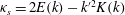 $\unicode[STIX]{x1D705}_{s}=2E(k)-k^{\prime 2}K(k)$
,
$\unicode[STIX]{x1D705}_{s}=2E(k)-k^{\prime 2}K(k)$
,
 $E(k)$
is the complete elliptic integral of the second kind,
$E(k)$
is the complete elliptic integral of the second kind,
 $a_{s}$
is the wave height defined as the vertical distance from trough to crest, and
$a_{s}$
is the wave height defined as the vertical distance from trough to crest, and
 $sc$
is a Jacobi elliptic function (recall that we have set
$sc$
is a Jacobi elliptic function (recall that we have set
 $\unicode[STIX]{x1D706}=2\unicode[STIX]{x03C0}$
). For antisymmetric waves, the transformation from Kinnersley’s parameter set to ours is given by
$\unicode[STIX]{x1D706}=2\unicode[STIX]{x03C0}$
). For antisymmetric waves, the transformation from Kinnersley’s parameter set to ours is given by
 $$\begin{eqnarray}H=\frac{\unicode[STIX]{x03C0}B}{K(k)},\quad c=\left(\frac{2T}{\unicode[STIX]{x03C0}\unicode[STIX]{x1D70C}c_{k}}\right)K(k)\,\text{cs}(B,k^{\prime })\,\text{nd}(B,k^{\prime }),\end{eqnarray}$$
where
 $cs$
and
$cs$
and
 $nd$
are Jacobi elliptic functions. Using Kinnersley’s expressions, we obtain the formula for the antisymmetric crest speed,
$nd$
are Jacobi elliptic functions. Using Kinnersley’s expressions, we obtain the formula for the antisymmetric crest speed,
 $$\begin{eqnarray}c_{k}=\left(\frac{4T\unicode[STIX]{x1D705}_{a}}{\unicode[STIX]{x1D70C}\unicode[STIX]{x1D706}}\right)^{1/2}\left(k^{\prime 2}+\frac{\unicode[STIX]{x1D705}_{a}^{2}a_{a}^{2}}{\unicode[STIX]{x1D706}^{2}}\right)^{-1/4}\left(1-\frac{k^{2}\unicode[STIX]{x1D706}^{2}}{\unicode[STIX]{x1D705}_{a}^{2}a_{a}^{2}}\right)^{-1/4},\quad \frac{a_{a}}{\unicode[STIX]{x1D706}}=\frac{k}{\unicode[STIX]{x1D705}_{a}}\,\text{nc}(B,k^{\prime }),\end{eqnarray}$$
with
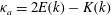 $\unicode[STIX]{x1D705}_{a}=2E(k)-K(k)$
, where
$\unicode[STIX]{x1D705}_{a}=2E(k)-K(k)$
, where
 $a_{a}$
is the wave height and
$a_{a}$
is the wave height and
 $nc$
is a Jacobi elliptic function.
$nc$
is a Jacobi elliptic function.
For our calculations we will fix
 $H$
and vary
$H$
and vary
 $c$
. We now demonstrate that in doing this we must always arrive at a limiting steady wave profile with a trapped bubble. If
$c$
. We now demonstrate that in doing this we must always arrive at a limiting steady wave profile with a trapped bubble. If
 $H$
is fixed it is straightforward to show that
$H$
is fixed it is straightforward to show that
 $B=HK(k)/\unicode[STIX]{x03C0}$
is monotonic increasing in
$B=HK(k)/\unicode[STIX]{x03C0}$
is monotonic increasing in
 $k$
. It can then be shown that
$k$
. It can then be shown that
 $a_{s}/\unicode[STIX]{x1D706}$
is a monotonic increasing function of
$a_{s}/\unicode[STIX]{x1D706}$
is a monotonic increasing function of
 $k$
and becomes unbounded as
$k$
and becomes unbounded as
 $k\rightarrow k_{0}$
, where
$k\rightarrow k_{0}$
, where
 $k_{0}$
satisfies
$k_{0}$
satisfies
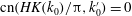 $\text{cn}(HK(k_{0})/\unicode[STIX]{x03C0},k_{0}^{\prime })=0$
(recall that
$\text{cn}(HK(k_{0})/\unicode[STIX]{x03C0},k_{0}^{\prime })=0$
(recall that
 $\text{sc}=\text{sn}/\text{cn}$
). Consequently
$\text{sc}=\text{sn}/\text{cn}$
). Consequently
 $a_{s}/\unicode[STIX]{x1D706}$
becomes arbitrarily large as
$a_{s}/\unicode[STIX]{x1D706}$
becomes arbitrarily large as
 $k\rightarrow k_{0}$
, and certainly larger than the threshold value stipulated by Kinnersley for self-intersecting waves (see his figure 3). We note that
$k\rightarrow k_{0}$
, and certainly larger than the threshold value stipulated by Kinnersley for self-intersecting waves (see his figure 3). We note that
 $c$
is a continuous function of
$c$
is a continuous function of
 $k$
over
$k$
over
 $[0,k_{0}]$
and so varying
$[0,k_{0}]$
and so varying
 $c$
corresponds to varying
$c$
corresponds to varying
 $k$
and hence we must always arrive at a limiting wave profile with a trapped bubble, and non-physical self-intersecting profiles beyond this. A similar argument holds for antisymmetric waves which must also eventually enclose a trapped bubble and then self-intersect.
$k$
and hence we must always arrive at a limiting wave profile with a trapped bubble, and non-physical self-intersecting profiles beyond this. A similar argument holds for antisymmetric waves which must also eventually enclose a trapped bubble and then self-intersect.
For completeness, we mention that Kinnersley showed that in the limit
 $k\rightarrow 1$
, symmetric waves approach a limiting profile, described neatly by Billingham (Reference Billingham2006) as the ‘string of beads’ solution, in which a periodic sequence of bulbous fluid beads, confined by upper and lower surfaces composed of parts of ellipses, are connected by asymptotically narrow neck regions providing a smooth transition from one bead to the next (see figure 5 of Kinnersley Reference Kinnersley1976). The gap between the necks on the upper and lower surface is asymptotically small, so that the waves are almost in contact. The wave profiles in this limit do not self-intersect provided that
$k\rightarrow 1$
, symmetric waves approach a limiting profile, described neatly by Billingham (Reference Billingham2006) as the ‘string of beads’ solution, in which a periodic sequence of bulbous fluid beads, confined by upper and lower surfaces composed of parts of ellipses, are connected by asymptotically narrow neck regions providing a smooth transition from one bead to the next (see figure 5 of Kinnersley Reference Kinnersley1976). The gap between the necks on the upper and lower surface is asymptotically small, so that the waves are almost in contact. The wave profiles in this limit do not self-intersect provided that
 $B$
is in the range
$B$
is in the range
 $[0,\unicode[STIX]{x03C0}/4]$
. At
$[0,\unicode[STIX]{x03C0}/4]$
. At
 $B=\unicode[STIX]{x03C0}/4$
the beads are semi-circular, and for
$B=\unicode[STIX]{x03C0}/4$
the beads are semi-circular, and for
 $B>\unicode[STIX]{x03C0}/4$
, the profiles self-intersect in the region of the necks. Noting that
$B>\unicode[STIX]{x03C0}/4$
, the profiles self-intersect in the region of the necks. Noting that
 $K\rightarrow \infty$
as
$K\rightarrow \infty$
as
 $k\rightarrow 1$
, the ‘string of beads’ solution may be obtained numerically using the present framework by fixing
$k\rightarrow 1$
, the ‘string of beads’ solution may be obtained numerically using the present framework by fixing
 $B$
and then increasing
$B$
and then increasing
 $k$
towards 1. The corresponding values of
$k$
towards 1. The corresponding values of
 $H$
and
$H$
and
 $c$
in this process come from the formulae in (C 1). We have confirmed that this procedure yields elliptic string-of-bead type profiles with neck regions which closely match Kinnersley’s asymptotic solution (72), although considerable numerical difficulties are encountered in computing these profiles for values of
$c$
in this process come from the formulae in (C 1). We have confirmed that this procedure yields elliptic string-of-bead type profiles with neck regions which closely match Kinnersley’s asymptotic solution (72), although considerable numerical difficulties are encountered in computing these profiles for values of
 $k$
very close to one.
$k$
very close to one.
Appendix D. Krein signature
Following MacKay & Saffman (Reference Mackay and Saffman1986) we compute the Krein signatures for linear perturbations by considering the sign of the total energy,
 $E$
, in one wave period in a frame of reference travelling at a nominated speed
$E$
, in one wave period in a frame of reference travelling at a nominated speed
 $c_{f}$
. The energy is defined as
$c_{f}$
. The energy is defined as
 $E=K+V-c_{f}P$
, where
$E=K+V-c_{f}P$
, where
 $K$
is the kinetic energy,
$K$
is the kinetic energy,
 $V$
is the potential energy and
$V$
is the potential energy and
 $P$
is the momentum transfer in the
$P$
is the momentum transfer in the
 $x$
direction through the ends of the reference frame. Individually, these terms are given as
$x$
direction through the ends of the reference frame. Individually, these terms are given as
 $$\begin{eqnarray}\left.\begin{array}{@{}c@{}}\displaystyle K=\int _{\mathscr{A}}\frac{1}{2}\unicode[STIX]{x1D70C}|\unicode[STIX]{x1D735}\unicode[STIX]{x1D719}|^{2}\,\text{d}A,\quad V=\int _{\mathscr{ S}_{U}}\unicode[STIX]{x1D6FE}[(1+\unicode[STIX]{x1D702}_{x}^{2})^{1/2}-1]\,\text{d}l+\int _{\mathscr{ S}_{L}}\unicode[STIX]{x1D6FE}[(1+\unicode[STIX]{x1D701}_{x}^{2})^{1/2}-1]\,\text{d}l,\\ \displaystyle P=\int _{\mathscr{A}}\unicode[STIX]{x1D70C}\unicode[STIX]{x1D719}_{x}\,\text{d}A,\end{array}\right\}\end{eqnarray}$$
where
 $\unicode[STIX]{x1D719}$
is the velocity potential,
$\unicode[STIX]{x1D719}$
is the velocity potential,
 $\mathscr{A}$
is the area between the upper and the lower surface contained in one wave period,
$\mathscr{A}$
is the area between the upper and the lower surface contained in one wave period,
 $\mathscr{S}_{U}$
,
$\mathscr{S}_{U}$
,
 $\mathscr{S}_{L}$
are the upper and lower surfaces in a period,
$\mathscr{S}_{L}$
are the upper and lower surfaces in a period,
 $\unicode[STIX]{x1D702}$
and
$\unicode[STIX]{x1D702}$
and
 $\unicode[STIX]{x1D701}$
are the displacements of the upper and lower surfaces respectively and
$\unicode[STIX]{x1D701}$
are the displacements of the upper and lower surfaces respectively and
 $l$
is the arc length along each surface. The Krein signature is positive if
$l$
is the arc length along each surface. The Krein signature is positive if
 $E>0$
and negative if
$E>0$
and negative if
 $E<0$
. The signature is particularly simple to calculate in the limit of small-amplitude sinusoidal waves. Assuming that the undisturbed surfaces are located at
$E<0$
. The signature is particularly simple to calculate in the limit of small-amplitude sinusoidal waves. Assuming that the undisturbed surfaces are located at
 $y=\pm H/2$
, to leading order we find using the divergence theorem for the
$y=\pm H/2$
, to leading order we find using the divergence theorem for the
 $K$
and
$K$
and
 $P$
integrals and the symmetry or antisymmetry of the linear waves for the
$P$
integrals and the symmetry or antisymmetry of the linear waves for the
 $V$
integral,
$V$
integral,
 $$\begin{eqnarray}\left.\begin{array}{@{}c@{}}\displaystyle K=\frac{1}{2}\unicode[STIX]{x1D70C}\int _{0}^{\unicode[STIX]{x1D706}}\unicode[STIX]{x1D719}\unicode[STIX]{x1D719}_{y}|_{y=H/2}-\unicode[STIX]{x1D719}\unicode[STIX]{x1D719}_{y}|_{y=-H/2}\,\text{d}x,\quad V=\frac{\unicode[STIX]{x1D6FE}}{2}\int _{0}^{\unicode[STIX]{x1D706}}\unicode[STIX]{x1D702}_{x}^{2}\,\text{d}x+\frac{\unicode[STIX]{x1D6FE}}{2}\int _{0}^{\unicode[STIX]{x1D706}}\unicode[STIX]{x1D701}_{x}^{2}\,\text{d}x,\\ \displaystyle P=\unicode[STIX]{x1D70C}\int _{0}^{\unicode[STIX]{x1D706}}\unicode[STIX]{x1D701}_{x}\unicode[STIX]{x1D719}|_{y=-H/2}-\unicode[STIX]{x1D702}_{x}\unicode[STIX]{x1D719}|_{y=H/2}\,\text{d}x.\end{array}\right\}\end{eqnarray}$$
We note that for linear sinusoidal waves, it follows from (2.13) that the conformal modulus and the physical sheet thickness coincide, so that
 $H=\bar{H}$
. According to linear stability theory (Taylor Reference Taylor1959), for waves with real wavenumber
$H=\bar{H}$
. According to linear stability theory (Taylor Reference Taylor1959), for waves with real wavenumber
 $\hat{k}$
(which we allow to be positive or negative) and frequency
$\hat{k}$
(which we allow to be positive or negative) and frequency
 $\hat{\unicode[STIX]{x1D714}}$
, travelling on a sheet of fluid otherwise at rest, we have the following results. For symmetric waves, we have the dispersion relation
$\hat{\unicode[STIX]{x1D714}}$
, travelling on a sheet of fluid otherwise at rest, we have the following results. For symmetric waves, we have the dispersion relation
 $\hat{\unicode[STIX]{x1D714}}^{2}=(\unicode[STIX]{x1D6FE}/\unicode[STIX]{x1D70C})\hat{k}^{3}\tanh (\hat{k}H/2)$
, and
$\hat{\unicode[STIX]{x1D714}}^{2}=(\unicode[STIX]{x1D6FE}/\unicode[STIX]{x1D70C})\hat{k}^{3}\tanh (\hat{k}H/2)$
, and
 $$\begin{eqnarray}\unicode[STIX]{x1D719}=\unicode[STIX]{x1D719}_{0}\cosh (\hat{k}y)\text{e}^{\text{i}(\hat{k}x-\hat{\unicode[STIX]{x1D714}}t)}+\text{c.c.},\quad \unicode[STIX]{x1D702}=\text{i}\hat{k}\unicode[STIX]{x1D719}_{0}\hat{\unicode[STIX]{x1D714}}^{-1}\sinh (\hat{k}H/2)\text{e}^{\text{i}(\hat{k}x-\hat{\unicode[STIX]{x1D714}}t)}+\text{c.c.},\end{eqnarray}$$
with
 $\unicode[STIX]{x1D701}=-\unicode[STIX]{x1D702}$
, where
$\unicode[STIX]{x1D701}=-\unicode[STIX]{x1D702}$
, where
 $\unicode[STIX]{x1D719}_{0}$
is an arbitrary complex constant, and c.c. denotes the complex conjugate. For antisymmetric waves, the dispersion relation is
$\unicode[STIX]{x1D719}_{0}$
is an arbitrary complex constant, and c.c. denotes the complex conjugate. For antisymmetric waves, the dispersion relation is
 $\hat{\unicode[STIX]{x1D714}}^{2}=(\unicode[STIX]{x1D6FE}/\unicode[STIX]{x1D70C})\hat{k}^{3}\,\text{coth}(\hat{k}H/2)$
, and we have
$\hat{\unicode[STIX]{x1D714}}^{2}=(\unicode[STIX]{x1D6FE}/\unicode[STIX]{x1D70C})\hat{k}^{3}\,\text{coth}(\hat{k}H/2)$
, and we have
 $$\begin{eqnarray}\unicode[STIX]{x1D719}=\unicode[STIX]{x1D719}_{0}\sinh (\hat{k}y)\text{e}^{\text{i}(\hat{k}x-\hat{\unicode[STIX]{x1D714}}t)}+\text{c.c.},\quad \unicode[STIX]{x1D702}=\text{i}\hat{k}\unicode[STIX]{x1D719}_{0}\hat{\unicode[STIX]{x1D714}}^{-1}\cosh (\hat{k}H/2)\text{e}^{\text{i}(\hat{k}x-\hat{\unicode[STIX]{x1D714}}t)}+\text{c.c.},\end{eqnarray}$$
with
 $\unicode[STIX]{x1D701}=\unicode[STIX]{x1D702}$
. For both symmetric and antisymmetric linear waves, we find
$\unicode[STIX]{x1D701}=\unicode[STIX]{x1D702}$
. For both symmetric and antisymmetric linear waves, we find
 $$\begin{eqnarray}K=V=2\unicode[STIX]{x03C0}\unicode[STIX]{x1D70C}|\unicode[STIX]{x1D719}_{0}|^{2}\frac{\hat{k}}{|\hat{k}|}\sinh (\hat{k}H),\quad P=4\unicode[STIX]{x03C0}\unicode[STIX]{x1D70C}\frac{\hat{k}^{2}}{\hat{\unicode[STIX]{x1D714}}|\hat{k}|}\sinh (\hat{k}H)|\unicode[STIX]{x1D719}_{0}|^{2}.\end{eqnarray}$$
The total energy as defined above is
 $$\begin{eqnarray}E=K+V-c_{f}P=4\unicode[STIX]{x03C0}\unicode[STIX]{x1D70C}\frac{\hat{k}}{{\hat{c}}|\hat{k}|}\sinh (\hat{k}H)|\unicode[STIX]{x1D719}_{0}|^{2}({\hat{c}}-c_{f}),\end{eqnarray}$$
where
 ${\hat{c}}=\hat{\unicode[STIX]{x1D714}}/\hat{k}$
. Consistent with § 4, and recalling that we are working in this paper with steady waves of period
${\hat{c}}=\hat{\unicode[STIX]{x1D714}}/\hat{k}$
. Consistent with § 4, and recalling that we are working in this paper with steady waves of period
 $2\unicode[STIX]{x03C0}$
, we decompose the wavenumber
$2\unicode[STIX]{x03C0}$
, we decompose the wavenumber
 $\hat{k}$
by writing
$\hat{k}$
by writing
 $\hat{k}=p+m$
, where
$\hat{k}=p+m$
, where
 $p$
is a real number in the range
$p$
is a real number in the range
 $[0,1)$
and
$[0,1)$
and
 $m$
is an integer. This allows us to relate the wave energy, and consequently the Krein signature, to the form of the perturbations adopted in (4.11). Furthermore, we may meaningfully attribute a Krein signature for a particular steady wave branch in the limit of zero amplitude by choosing
$m$
is an integer. This allows us to relate the wave energy, and consequently the Krein signature, to the form of the perturbations adopted in (4.11). Furthermore, we may meaningfully attribute a Krein signature for a particular steady wave branch in the limit of zero amplitude by choosing
 $c_{f}=c_{s}$
for symmetric waves and
$c_{f}=c_{s}$
for symmetric waves and
 $c_{f}=c_{a}$
for antisymmetric waves. Following MacKay & Saffman (Reference Mackay and Saffman1986), we calculate the Krein signature
$c_{f}=c_{a}$
for antisymmetric waves. Following MacKay & Saffman (Reference Mackay and Saffman1986), we calculate the Krein signature
 $s_{K}$
by scrutinising the sign of
$s_{K}$
by scrutinising the sign of
 $E$
. As in the main body of the paper we set
$E$
. As in the main body of the paper we set
 $\unicode[STIX]{x1D6FE}=\unicode[STIX]{x1D70C}=1$
. For symmetric perturbations we have
$\unicode[STIX]{x1D6FE}=\unicode[STIX]{x1D70C}=1$
. For symmetric perturbations we have
 $$\begin{eqnarray}s_{K}=\text{sgn}[\unicode[STIX]{x1D708}\,\text{Im}(\unicode[STIX]{x1D70E}_{s,m}^{\unicode[STIX]{x1D708}})]=\text{sgn}\left[\frac{{\hat{c}}-c_{f}}{{\hat{c}}}\right]=\text{sgn}[[\hat{k}^{3}\tanh (H\hat{k}/2)]^{1/2}-\unicode[STIX]{x1D708}\hat{k}c_{f}],\end{eqnarray}$$
where
 $\unicode[STIX]{x1D708}=\pm 1$
and
$\unicode[STIX]{x1D708}=\pm 1$
and
 $\hat{k}=p+m$
and
$\hat{k}=p+m$
and
 $c_{f}=c_{s}$
or
$c_{f}=c_{s}$
or
 $c_{a}$
. For antisymmetric perturbations, we have
$c_{a}$
. For antisymmetric perturbations, we have
 $$\begin{eqnarray}s_{K}=\text{sgn}[\unicode[STIX]{x1D708}\,\text{Im}(\unicode[STIX]{x1D70E}_{a,m}^{\unicode[STIX]{x1D708}})]=\text{sgn}\left[\frac{{\hat{c}}-c_{f}}{{\hat{c}}}\right]=\text{sgn}[[\hat{k}^{3}\,\text{coth}(H\hat{k}/2)]^{1/2}-\unicode[STIX]{x1D708}\hat{k}c_{f}],\end{eqnarray}$$
for
 $c_{f}=c_{s}$
or
$c_{f}=c_{s}$
or
 $c_{a}$
.
$c_{a}$
.
To provide an example, we consider the stability calculation for antisymmetric base waves with
 $H=1$
shown in figure 8. Using the preceding formulae, we compute the Krein signatures for the eigenvalues shown in the figure at
$H=1$
shown in figure 8. Using the preceding formulae, we compute the Krein signatures for the eigenvalues shown in the figure at
 $c-c_{a}=0$
. The results are presented in table 2.
$c-c_{a}=0$
. The results are presented in table 2.


