


1 Introduction
A thin film coating a flat substrate in a position where gravity tends to pull off the fluid may lead to amplifying disturbances of the interface, possibly leading to dripping. For thin films flowing down the underneath of inclined surfaces, a complete description of this phenomenon remains to be assessed and we aim at having a detailed characterization of the intermediate steps leading from a flat film to the dripping of drops.
A horizontal flat interface separating a heavier fluid and a lighter fluid in two semi-infinite regions will deform with time if the overlaying fluid is the heaviest one (Rayleigh Reference Rayleigh1882; Taylor Reference Taylor1950). Adding surface tension stabilizes the small-scale disturbances of the interface, but large-scale disturbances are always unstable (Chandrasekhar Reference Chandrasekhar1961). The instability is driven by a competition between gravity, which pulls the heavy fluid down, and surface tension that tends to restore a flat interface and pushes it back. This instability is of prime concern when coating surfaces e.g. with paint or lubricants as coating irregularities or detachment of droplets may appear. As such, many studies have focused on means of controlling or suppressing the growth of pendant drops. This can be achieved, for example, by surface tension gradients arising from a temperature difference across the thin film or from the evaporation of the solvent in a multicomponent liquid (Burgess et al. Reference Burgess, Juel, McCormick, Swift and Swinney2001; Bestehorn & Merkt Reference Bestehorn and Merkt2006; Alexeev & Oron Reference Alexeev and Oron2007; Weidner, Schwartz & Eres Reference Weidner, Schwartz and Eres2007). The Rayleigh–Taylor instability can also be controlled by high-frequency vibrations of the substrate (Lapuerta, Mancebo & Vega Reference Lapuerta, Mancebo and Vega2001; Sterman-Cohen, Bestehorn & Oron Reference Sterman-Cohen, Bestehorn and Oron2017) or by the application of an electric field (Barannyk, Papageorgiou & Petropoulos Reference Barannyk, Papageorgiou and Petropoulos2012; Cimpeanu, Papageorgiou & Petropoulos Reference Cimpeanu, Papageorgiou and Petropoulos2014).
When the film is located underneath a substrate, its thickness is limited by gravity to typically a few millimetres, and the flow is thus strongly confined which enhances viscous dissipation. In this situation, regular patterns ranging from hexagons to squares are observed (Fermigier et al. Reference Fermigier, Limat, Wesfreid, Boudinet and Quilliet1992). This problem is usually tackled by assuming that the wavelength of the perturbations is larger than the film thickness and that the Reynolds number based on the film thickness is small, leading to the lubrication approximation, (Kapitza Reference Kapitza and Haar1965; Babchin et al. Reference Babchin, Frenkel, Levich and Sivashinsky1983; Chang Reference Chang1994). These patterns are periodic nonlinear structures composed of a repetition of lenses that, assuming a linearized expression of the curvature, do not saturate but slowly grow algebraically (Lister, Rallison & Rees Reference Lister, Rallison and Rees2010). For sufficiently small initial thicknesses, and considering instead the full curvature, the lenses asymptotically approach axisymmetric pendant drop shapes (Marthelot et al. Reference Marthelot, Strong, Reis and Brun2018). Spontaneous sliding of the droplets across the planar surface of the substrate can occur (Glasner Reference Glasner2007) due to a symmetry-breaking instability (Dietze, Picardo & Narayanan Reference Dietze, Picardo and Narayanan2018).
When the substrate is tilted, the film is still unstable but has a smaller growth rate as gravity is projected orthogonally to the substrate. The tangential component of the gravity then induces a flow that advects perturbations and, depending on the inclination angle and the film thickness, the instability can switch from convective to absolute. Brun et al. (Reference Brun, Damiano, Rieu, Balestra and Gallaire2015) experimentally show the agreement between the linear prediction of the onset of the absolute instability and the onset of dripping. Inertial effects and viscous extensional stresses are added to the latter stability prediction by Scheid, Kofman & Rohlfs (Reference Scheid, Kofman and Rohlfs2016). Kofman et al. (Reference Kofman, Rohlfs, Gallaire, Scheid and Ruyer-Quil2018) demonstrate using a hierarchy of computational models that the absolute regime does not predict the onset of two-dimensional dripping satisfactorily.
To date, experiments are mostly transient in nature since a finite volume of fluid was released (Fermigier et al. Reference Fermigier, Limat, Wesfreid, Boudinet and Quilliet1992; Brun et al. Reference Brun, Damiano, Rieu, Balestra and Gallaire2015), with the noticeable exceptions of Rietz et al. (Reference Rietz, Scheid, Gallaire, Kofman, Kneer and Rohlfs2017), in which the wall normal gravity component is replaced by a centrifugal acceleration, and Charogiannis et al. (Reference Charogiannis, Denner, van Wachem, Kalliadasis, Scheid and Markides2018). The difference between transient release dynamics and alimented flows appears to be significant. For the classical Rayleigh–Taylor instability under a flat ceiling, permanent-fed experiments through a porous supply have been mostly done in a horizontal annular geometry, which effectively mimics a one-dimensional substrate (Limat et al. Reference Limat, Jenffer, Dagens, Touron, Fermigier and Wesfreid1992; Abdelall et al. Reference Abdelall, Abdel-Khalik, Sadowski, Shin and Yoda2006). This latter configuration gives rise to a particularly rich and complex dynamics of interacting dripping drops or continuous columns (Pirat et al. Reference Pirat, Mathis, Maissa and Gil2004; Brunet, Flesselles & Limat Reference Brunet, Flesselles and Limat2007), and may even lead to massive dripping within corrugated sheets (Yoshikawa et al. Reference Yoshikawa, Mathis, Satoh and Tasaka2019).
We thus propose a new experimental set-up, combining a permanent liquid supply to a tilted and flat coated surface, in contrast to recent studies on cylindrical and spherical substrates displaying a stabilizing effect on the film thanks to drainage-induced thinning and stretching (Balestra et al. Reference Balestra, Kofman, Brun, Scheid and Gallaire2018a; Balestra, Nguyen & Gallaire Reference Balestra, Nguyen and Gallaire2018b). In order to overcome the limitation of a transient experiment, we impose a constant flow rate so that the flow can reach a steady state or an asymptotic behaviour. The Reynolds number of our flow is as small as possible, using very viscous oils, as simple non-inertial models already incur complex nonlinearities. The experiment allows us to explore a wide range of parameters, i.e. all angles from vertical to horizontal and large variations of the film thickness. In this experiment we can observe a whole variety of patterns, from almost unperturbed flat films to heavy rains of oil droplets (Lerisson et al. Reference Lerisson, Ledda, Balestra and Gallaire2019). In particular, we study the stability of the flat film solution, and identify a range of parameters within which the film destabilizes into long rivulet structures.
In this work, we study the steady patterns emerging from natural and external forcing, describing the behaviour of such a thin film continuously flowing under an inclined flat substrate with a combination of experiments, numerical simulations and linear stability theory. The experimental set-up is described in § 2 together with the measurement techniques, which are illustrated by a first spatially forced film, as well as the necessary scalings. Section 3 is devoted to a theoretical spatial stability analysis, which is compared to experimental measurements. Section 4 is devoted to the measurements of a freely flowing film together with numerical simulations. Again, the results are compared to the predictions of a local linear stability analysis. We finally discuss the nature of fully nonlinear static rivulet solutions, which naturally emerge in these steady patterns. We show that they have the shape of purely two-dimensional (2-D) pendent drops, known to adopt the shape of an elastica. In this paper, we only focus on steady flows; the dynamics and transients that lead to those patterns are not investigated.
2 Methods
2.1 Experimental apparatus
The experiment (figure 1) consists of injecting a Newtonian fluid on the underside of an inclined flat substrate with a constant flow rate. The substrate is a glass plate (dimensions 600 × 300 mm) attached on an orientable structure, forming an angle  $\unicode[STIX]{x1D703}$ with the vertical axis. In the present study,
  $\unicode[STIX]{x1D703}$ is varied from
  $20^{\circ }$ to
  $55^{\circ }$. The fluid is silicon oil (Bluestar Silicons 47V1000) of measured viscosity
  $\unicode[STIX]{x1D707}=1089~\text{mPa}~\text{s}$, density
  $\unicode[STIX]{x1D70C}=974~\text{kg}~\text{m}^{-3}$, kinematic viscosity
  $\unicode[STIX]{x1D708}=\unicode[STIX]{x1D707}/\unicode[STIX]{x1D70C}=1.12\times 10^{-3}~\text{m}^{2}~\text{s}^{-1}$ and surface tension
  $\unicode[STIX]{x1D6FE}=21~\text{mN}~\text{m}^{-1}$. The fluid is injected through a horizontal slit-shaped inlet from a closed reservoir fully filled with oil and connected to an open reservoir. The open reservoir, placed above the inlet, is constantly filled and the height of the liquid is kept constant by the use of an overflow. The oil flowing down the substrate is collected in a home reservoir and loops back during the experiment. The flow rate is set by varying the height difference
  $H$ between the closed reservoir and the open reservoir, giving an upper bound of
  $1.7\times 10^{-3}~\text{kg}~\text{s}^{-1}$ (corresponding to a film of equivalent thickness
  $h_{N}=1.5~\text{mm}$) and down to arbitrary low flux values. The flow rate is measured by collecting the oil leaving the substrate during three minutes, and weighing it. Before any experiment, the substrate is prewetted to ensure a zero contact angle (total wetting). All the experimental results presented here are measured on stationary films, i.e. the thickness reaches a stationary state. A forcing blade, consisting of a laser-cut rectangle with a sinusoidal long edge (sketched in figure 1b), can be placed just below the inlet. The blade does not occlude the flow and is spaced from the glass by lateral spacers. An acute angle (approximately
  $30^{\circ }$) is introduced between the blade and the glass. The liquid fully fills the created gap underneath the blade and slightly spreads spanwise. The blade is always larger than the initial inlet and the lateral spreading remains in the sinusoidal part. The modified width
  $W_{i}^{\ast }$ is measured systematically, resulting in a new equivalent thickness
  $h_{N}$. The sine wave has a peak-to-peak amplitude of 0.5 mm and the spacers of 1 mm which should be projected with the acute angle, giving a perturbation of amplitude
  ${\approx}250~\unicode[STIX]{x03BC}\text{m}$. The blade acts as a new initial condition and is taken as a new inlet reference for the flow.

Figure 1. (a) Sketch of the experimental apparatus, (b) details of the forcing blade used to perturb the film and (c) picture of the experimental apparatus. Rivulets can be observed under the glass plate.
We measure the film thickness  ${\hat{h}}$ with a confocal chromatic sensor (STIL CCS) located on the upper (dry) side of the substrate. The sensor gives a point thickness measurement at an acquisition rate of 500 Hz. The sensor is attached on a two-axis linear stage and we perform horizontal scans of length
  $\hat{L}_{s}=200~\text{mm}$ in the
  ${\hat{y}}$ direction (4 s per scan). The sensor performs two scans back and forth and returns to its initial position; we thus obtain the thickness profile twice. We compute the difference between these two measurements and remove errors by discarding values with a difference greater than
  $50~\unicode[STIX]{x03BC}\text{m}$ and values where the variation between successive points is larger than
  $500~\unicode[STIX]{x03BC}\text{m}$. We map the whole substrate every 10, 30 or 50 mm in the
  $\hat{x}$ direction. The optical measurement cannot access to film thickness distributions with a surface steepness higher than
  $40^{\circ }$, following the STIL CCS specifications.
In addition, we set up another acquisition method based on the absorption of a coloured liquid. The same silicon oil is mixed with Sudan Black B that has a peak of absorption at 595 nm. A flat screen of light covers the whole glass plate. A camera (Nikon D850 with a Nikon 50 mm lens) is then attached on the structure at 85 cm from the glass plate, giving a resolution of  $7.6~\text{pixels}~\text{mm}^{-1}$. The luminance measured by each pixel is related to the thickness with the Beer–Lambert law (Limat et al. Reference Limat, Jenffer, Dagens, Touron, Fermigier and Wesfreid1992)
 $$\begin{eqnarray}{\hat{h}}(\hat{x},{\hat{y}},\hat{t})=\frac{1}{C}\log \left(\frac{I_{0}(\hat{x},{\hat{y}})}{I(\hat{x},{\hat{y}},\hat{t})}\right),\end{eqnarray}$$
 where  $I_{0}$ is the initial luminance measured without any liquid,
  $I$ the luminance at time
  $t$ and
  $C$ is a constant value that is determined with a calibration procedure that consists in measuring the luminance through a known wedge.
Finally, we can optically enhance film perturbations and identify phases and patterns. The visualization technique is based on the distortion of a regular grid through the transparent liquid film. The grid has been fixed to a square light screen, placed behind the glass plate. In order to reduce the parallax effect, we placed the camera at a distance of 5 m from the plate.
2.2 Scalings
The reduced capillary length is given by a balance between surface tension and gravity projected perpendicularly to the substrate. In order to conveniently scale the in-plane  $(\hat{x},{\hat{y}})$ length scales, we define the reduced capillary length
  $\ell _{c}^{\ast }$,
 $$\begin{eqnarray}\ell _{c}^{\ast }=\frac{\ell _{c}}{\sqrt{\sin \unicode[STIX]{x1D703}}},\end{eqnarray}$$
 where  $\ell _{c}=\sqrt{\unicode[STIX]{x1D6FE}/\unicode[STIX]{x1D70C}g}=1.49~\text{mm}$ is the capillary length. With the angle variation, it gives a range for the reduced capillary length of
  $1.85~\text{mm}<\ell _{c}^{\ast }<2.54~\text{mm}$. For a given volumetric flow rate
  $q$, we can define the Nusselt flat film thickness
  $h_{N}$, used to define the wall-normal
  $(\hat{z})$ length scale
 $$\begin{eqnarray}h_{N}=\left(\frac{3\unicode[STIX]{x1D708}q}{{\hat{W}}_{i}g\cos \unicode[STIX]{x1D703}}\right)^{1/3},\end{eqnarray}$$
 which is the constant thickness of an equivalent flat viscous film of width  ${\hat{W}}_{i}$, assuming a half-plane Poiseuille flow in the
  $\boldsymbol{e}_{x}$ direction and no flow in the
  $\boldsymbol{e}_{y}$ and
  $\boldsymbol{e}_{z}$ directions. In this study,
  $h_{N}$ is varied from 0.5 to 1.5 mm.
3 Forced dynamics
For a certain range of  $\unicode[STIX]{x1D703}$ and
  $h_{N}$, the flat film is convectively unstable (Brun et al. Reference Brun, Damiano, Rieu, Balestra and Gallaire2015); perturbations grow and are advected downstream. We first study the film response to a spatially periodic forcing.
3.1 Experimental results
We place a horizontal blade with a sinusoidal-shaped edge against the substrate. The height of the liquid film is imposed by the distance separating the blade and the substrate. The blade is located just below the inlet (at  $x=0$) and imposes an inlet condition with dimensionless horizontal wave vector
  $k_{f}$ and corresponding wavelength
  $\unicode[STIX]{x1D706}_{f}$ in the
  $y$ direction, with
  $k_{f}=2\unicode[STIX]{x03C0}/\unicode[STIX]{x1D706}_{f}$. We design a set of blades for a range of spacings that goes from 5 to 1 cm, leading to a variation of the horizontal wave vector
  $0.32<k_{f}<1.44$ for an inclination angle
  $\unicode[STIX]{x1D703}=20^{\circ }$, and
  $0.15<k_{f}<0.75$ for
  $\unicode[STIX]{x1D703}=39^{\circ }$.

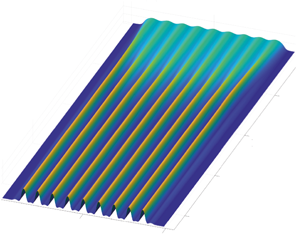
Figure 2. Film thickness for  $\unicode[STIX]{x1D703}=39^{\circ }$ and
  $h_{N}=1515~\unicode[STIX]{x03BC}\text{m}$ (
 $u=1.5$), forcing at the optimal wavelength
  $\unicode[STIX]{x1D706}_{f}=8.90$. The thickness is measured with the absorption method and normalized by the flat film thickness
  $h_{N}$.
Figure 2 shows a typical measurement of the entire film thickness  $h$ by absorption, with
  $h_{N}=1515~\unicode[STIX]{x03BC}\text{m}$ and
  $\unicode[STIX]{x1D703}=39^{\circ }$. The film is flowing in the positive
  $x$ direction. The sinusoidal shape of the forcing propagates downwards, forming mainly streamwise phase lines. The amplitude of the response grows with
  $x$ between
  $x=0$ and
  $x=50$ in a self-preserving manner. Between
  $x=50$ and
  $x=200$, the amplitude reaches a plateau and the shape is no longer sinusoidal. Beyond
  $x=200$, the shapes start to develop streamwise oscillations. These oscillations are unsteady and their occurrence is not studied here. The flow rate and inclination angle chosen for this particular case of figure 2 are larger than the ones considered in the rest of the study, in which the responses are always stationary.

Figure 3. Evolution of the film thickness for  $\unicode[STIX]{x1D703}=20^{\circ }$ and
  $h_{N}=560~\unicode[STIX]{x03BC}\text{m}$ (
 $u=12.5$) and forced wavelengths: (a)
  $\unicode[STIX]{x1D706}_{f}=4.37$; (b)
  $\unicode[STIX]{x1D706}_{f}=7.87$; and (c)
  $\unicode[STIX]{x1D706}_{f}=19.67$. The thickness is measured using the STIL CCS scanning every 10 mm (in dimensionless form
  $\unicode[STIX]{x1D6FF}_{x}=10~\text{mm}/\ell _{c}^{\ast }=3.9$). The red line shows the imposed inlet thickness at
  $x=0$.
We first focus on the spatial growth phase. We follow the evolution of the thickness for several position  $x$ between
  $x=19.7$ and
  $x=118$ for different wavelengths and a fixed flow rate. We observe three regimes.
Figure 3(a) shows the forcing propagating downstream with a decreasing amplitude, until vanishing around  $x=50$. The film is then flat except on its lateral sides where thickness perturbations with respect to a flat condition propagate and grow. In panels (b,c), the forcing propagates in all the domain with an amplitude that slightly increases in the streamwise direction. On the lateral sides, the signal is deformed and this deformation propagates inward. In panel (c), the profile never follows the forced wavelength but follows
  $\unicode[STIX]{x1D706}_{f}/2$; similarly the obtained pattern is deformed when penetrating away from the lateral sides.
3.2 Linear stability
We compare these experimental results to the linear prediction obtained from the dispersion relation of the linearized thin film equation. The nonlinear thin film equation is based on the assumption that the orthogonal derivatives  $(\hat{z})$ are much larger than the in-plane
  $(\hat{x},{\hat{y}})$ derivatives. We define the characteristic time scale
  $\unicode[STIX]{x1D70F}$,
 $$\begin{eqnarray}\unicode[STIX]{x1D70F}=\frac{\unicode[STIX]{x1D708}\ell _{c}^{2}}{h_{N}^{3}g\sin ^{2}\unicode[STIX]{x1D703}}.\end{eqnarray}$$
 Spatial directions  $\hat{x}$ and
  ${\hat{y}}$ are non-dimensionalized by
  $\ell _{c}^{\ast }$, thickness
  ${\hat{h}}$ by
  $h_{N}$ and time
  $\hat{t}$ by
  $\unicode[STIX]{x1D70F}$,
 $$\begin{eqnarray}\displaystyle & x=\hat{x}/\ell _{c}^{\ast }, & \displaystyle\end{eqnarray}$$
 $$\begin{eqnarray}\displaystyle & y={\hat{y}}/\ell _{c}^{\ast }, & \displaystyle\end{eqnarray}$$
 $$\begin{eqnarray}\displaystyle & h={\hat{h}}/h_{N}, & \displaystyle\end{eqnarray}$$
 $$\begin{eqnarray}\displaystyle & t=\hat{t}/\unicode[STIX]{x1D70F}. & \displaystyle\end{eqnarray}$$
Following previous works (Ruschak Reference Ruschak1978; Wilson Reference Wilson1982; Kheshgi, Kistler & Scriven Reference Kheshgi, Kistler and Scriven1992; Weinstein & Ruschak Reference Weinstein and Ruschak2004), the full curvature term is retained. In non-dimensional form, the equation reads
 $$\begin{eqnarray}\frac{\unicode[STIX]{x2202}h}{\unicode[STIX]{x2202}t}+\tilde{\ell _{c}}^{\ast }\cot (\unicode[STIX]{x1D703})h^{2}\frac{\unicode[STIX]{x2202}h}{\unicode[STIX]{x2202}x}+\frac{1}{3}\unicode[STIX]{x1D735}\boldsymbol{\cdot }(h^{3}(\unicode[STIX]{x1D735}h+\unicode[STIX]{x1D735}\unicode[STIX]{x1D705}))=0,\end{eqnarray}$$
 where  $\unicode[STIX]{x1D735}$ operates in the
  $(x,y)$ plane,
  $\tilde{\ell _{c}}^{\ast }=\ell _{c}^{\ast }/h_{N}$ and
  $\unicode[STIX]{x1D705}$ is the mean curvature
 $$\begin{eqnarray}\unicode[STIX]{x1D705}=\frac{{\displaystyle \frac{\unicode[STIX]{x2202}^{2}h}{\unicode[STIX]{x2202}x^{2}}}\left(1+{\displaystyle \frac{\unicode[STIX]{x2202}h}{\unicode[STIX]{x2202}y}}^{2}\right)+{\displaystyle \frac{\unicode[STIX]{x2202}^{2}h}{\unicode[STIX]{x2202}y^{2}}}\left(1+{\displaystyle \frac{\unicode[STIX]{x2202}h}{\unicode[STIX]{x2202}x}}^{2}\right)-2{\displaystyle \frac{\unicode[STIX]{x2202}h}{\unicode[STIX]{x2202}x}}{\displaystyle \frac{\unicode[STIX]{x2202}h}{\unicode[STIX]{x2202}y}}{\displaystyle \frac{\unicode[STIX]{x2202}^{2}h}{\unicode[STIX]{x2202}x\unicode[STIX]{x2202}y}}}{\left(1+{\displaystyle \frac{\unicode[STIX]{x2202}h}{\unicode[STIX]{x2202}x}}^{2}+{\displaystyle \frac{\unicode[STIX]{x2202}h}{\unicode[STIX]{x2202}y}}^{2}\right)^{3/2}}.\end{eqnarray}$$
 In the following, we focus on the emergence of steady states in response to a stationary forcing. We thus assume no time variations and we consider a stationary perturbation with respect to the flat film condition. Introducing  $h=1+\unicode[STIX]{x1D716}h^{\prime }$ with a steady perturbation
  $h^{\prime }\propto \text{e}^{\text{i}\boldsymbol{k}\boldsymbol{\cdot }\boldsymbol{x}}$ where
  $\boldsymbol{k}=(k_{x},k_{y})$, equation (3.6) is linearized to obtain the dispersion relation
 $$\begin{eqnarray}\frac{\text{i}}{3}(|\boldsymbol{k}|^{2}-|\boldsymbol{k}|^{4})+\underbrace{\cot \unicode[STIX]{x1D703}\tilde{\ell _{c}}^{\ast }}_{u}k_{x}=0,\end{eqnarray}$$
 where  $u$ is the coefficient of a linear phase advection which corresponds to the surface film velocity that advects the linear perturbations downstream.
We neglect the lateral side and assume the forcing and the response to be homogeneous and purely in the spanwise direction, i.e.  $\text{Im}(k_{y})=0$ and
  $k_{y}=k_{f}$. For each forcing wavelength
  $2\unicode[STIX]{x03C0}/k_{y}$, we thus obtain the corresponding spatial growth rate
  $k_{x}(k_{y})$ by solving the equation
 $$\begin{eqnarray}(k_{y}^{2}-k_{y}^{4})+(k_{x}^{4}+k_{x}^{2}+2k_{x}^{2}k_{y}^{2})-3\text{i}uk_{x}=0,\end{eqnarray}$$
 which is a fourth-order polynomial in  $k_{x}$ which can be solved for as a function of
  $k_{y}$. Among all the four roots of the complex polynomial, we discard solutions which have
  $\text{Re}(k_{x})\neq 0$, i.e. solutions that oscillate along the streamwise direction. There is only one branch that corresponds to a purely growing, downstream amplified, spatial wave (
 $\text{Re}(k_{x})=0$). The maximum growth rate is not attained exactly at
  $k_{y}=1/\sqrt{2}$, as for the temporal growth rate (Brun et al. Reference Brun, Damiano, Rieu, Balestra and Gallaire2015) but it deviates by no more than 0.2 % for the cases considered in this study (see figure 11 in appendix A). In such a convective situation where we have
  $u>c_{g0}$ with
  $u=12.5$ (figure 3) and the absolute group velocity
  $c_{g0}=0.54$ (Brun et al. Reference Brun, Damiano, Rieu, Balestra and Gallaire2015), the streamwise growth of spanwise wavenumbers strongly resembles their temporal growth, a property similar to the Gaster transformation (Gaster Reference Gaster1962), though not directly related to it.
Experimentally, we measure the spatial growth rate and compare it to  $\text{Im}(k_{x})$ by measuring the amplitude
  $A(x)$ defined by
 $$\begin{eqnarray}A(x)=\sqrt{\int _{{\hat{y}}=0.2\hat{L}_{s}}^{{\hat{y}}=0.8\hat{L}_{s}}({\hat{h}}(x,y)-h_{N})^{2}\,\text{d}{\hat{y}}},\end{eqnarray}$$
 along the  $x$ direction. Results corresponding to the three cases presented in figure 3 are plotted in figure 4(a–c) (black crosses) in log scale as a function of
  $x$ along with the theoretical prediction (red lines) normalized by the first measurement. Panel (a) shows an exponentially decreasing amplitude up to
  $x=40$ before saturating to a lower noisy value. The decrease is well captured by the linear prediction (3.9). Panel (b) shows an exponentially increasing amplitude all over the
  $x$ measurement range which is well predicted by the theory. In panel (c) the amplitude is also following an exponential increase but at a rate that is much faster than the prediction for the corresponding wavelength; we also plot the growth predicted for the superharmonic wavelength (
 $\unicode[STIX]{x1D706}=\unicode[STIX]{x1D706}_{f}/2$) that almost perfectly matches the experimental measurement.

Figure 4. (d) Theoretical (red curve) and experimental (black crosses) spatial growth rates as a function of the forcing wavelength  $k_{y}$; yellow curve is the theoretical prediction for the harmonic
  $2k_{y}$. (a–c) Experimental amplitudes (crosses) and theoretical prediction (red lines) for the three cases presented in figure 3. The yellow line in panel (c) is the prediction for the harmonic
  $2k_{y}$. The corresponding measurements are reported as points
  $A$,
$A$,  $B$ and
  $C$ in panel (d).
The measurements are summarized in figure 4(d) where we plot the growth rates for  $0<k_{y}<2$. The predicted growth rate (red line, solution of (3.9)) is in excellent agreement with the experimental data (crosses). In addition, we plot in yellow the solution of (3.9) for
  $k_{y}=2k_{f}$. The measured points labelled
  $A$,
$A$,  $B$ and
  $C$ correspond to the full measurements showed in panels (a–c).
The linear dispersion relation shows a cutoff wavenumber at  $k_{y}=1$, corresponding to a dimensional wavelength of
  $2\unicode[STIX]{x03C0}\ell _{c}^{\ast }$. So when we increase the angle
  $\unicode[STIX]{x1D703}$, the range of unstable wavelength decreases. The spatial growth rate
  $k_{x}$ is a decreasing function of
  $u$ which depends on the two parameters,
  $h_{N}$ and
  $\unicode[STIX]{x1D703}$. Increasing
  $\unicode[STIX]{x1D703}$ (toward a more horizontal substrate) leads to a decrease of
  $u$ and an increase of
  $k_{x}$. If the forced wavelength is unstable, its amplitude grows and saturates close to the inlet. Similarly, increasing
  $h_{N}$ leads to a decrease of
  $u$ and an increase of
  $k_{x}$, while the dimensional velocity of the flat film surface is, however, increased. This comes from the time scale that is inversely proportional to
  $h_{N}^{3}$; while perturbations are advected faster with an increase of
  $h_{N}$ (that would lead to a smaller spatial growth rate), they are amplified even more (resulting in the spatial growth rate eventually to increase).
4 Natural dynamics
Even without the inlet device shown in figure 1(b), thickness perturbations with respect to the flat film grow from the sides and may invade the entire domain, as shown in figure 5(a,c,e). Far from the sides, the film thickness is constant for all  $x$ in panels (a,c). In panel (e), the perturbation invades the entire film. The side perturbations penetrate inside while also being advected downstream. In panels (b,d,f), we perturb the film by placing a small cylinder (of diameter 2 mm) in the middle of the film and close to the inlet. The perturbation is stationary and propagates both downstream and in the spanwise direction. The perturbation amplitude grows with the streamwise direction and high amplitude variations cannot be captured in panel (f).

Figure 5. Evolution of the film thickness without forcing in case of: (a)  $h_{N}=678~\unicode[STIX]{x03BC}\text{m}$,
  $\unicode[STIX]{x1D703}=20^{\circ }$ (
 $u=10.3$); (c)
  $h_{N}=1142~\unicode[STIX]{x03BC}\text{m}$,
  $\unicode[STIX]{x1D703}=20^{\circ }$ (
 $u=6.1$); (e)
  $h_{N}=726~\unicode[STIX]{x03BC}\text{m}$,
  $\unicode[STIX]{x1D703}=40^{\circ }$ (
 $u=3.0$). Evolution of the film thickness with a stationary localized forcing in case of: (b)
  $h_{N}=1334~\unicode[STIX]{x03BC}\text{m}$,
  $\unicode[STIX]{x1D703}=20^{\circ }$ (
 $u=5.2$); (d)
  $h_{N}=390~\unicode[STIX]{x03BC}\text{m}$,
  $\unicode[STIX]{x1D703}=40^{\circ }$ (
 $u=5.7$); (f)
  $h_{N}=1357~\unicode[STIX]{x03BC}\text{m}$,
  $\unicode[STIX]{x1D703}=30^{\circ }$ (
 $u=2.7$). The red lines are the theoretical predictions for the front propagation computed with the help of (3.9).
In this context of highly advected perturbations, we look for the steady front of the region invaded by the perturbation.
4.1 ‘Spatio-spatial’ stability analysis
Instead of focusing on the spatio-temporal growth and propagation of this wave packet in two dimensions of space, we assume steady patterns and only consider a ‘spatio-spatial’ wave packet growth. The classical absolute/convective calculation can be generalized to the streamwise spatial growth of spanwise spatially periodic disturbances. In this analogy,  $x$ plays the role of time and
  $k_{x}$ that of the complex frequency while
  $k_{y}$ is the complex spatial wavenumber; the dispersion relation (3.9) now takes into account for complex wavenumbers,
  $D(k_{x},k_{y},u)=0$.
We can make an analogy with a spatio-temporal analysis, where the front is defined by a particular ray  $x/t=v$ for which the perturbation is marginally stable, as
  $t\rightarrow \infty$ (Huerre & Monkewitz Reference Huerre and Monkewitz1990; Van Saarloos Reference Van Saarloos2003; King et al. Reference King, Weinstein, Zaretzky, Cromer and Barlow2016). In this approach, the front is the velocity, i.e. the amount of space per unit of time, at which the perturbation spreads in the domain while being advected. Here, we look for the front angle
  $y/x=\tan (\unicode[STIX]{x1D719})$, i.e. the amount of spanwise space per unit of streamwise space, separating the perturbed domain from the region where the perturbation does not propagate, as
  $x\rightarrow \infty$.
We then numerically determine the angle  $\unicode[STIX]{x1D719}$ for which
  $\unicode[STIX]{x2202}\text{Im}(k_{x})/\unicode[STIX]{x2202}\text{Im}(k_{y})=\tan (\unicode[STIX]{x1D719})$, imposing
  $\unicode[STIX]{x2202}\text{Re}(k_{x})/\unicode[STIX]{x2202}\text{Im}(k_{y})=0$. It consists of the extraction of the relevant roots from a complex fourth-order polynomial, which is performed using the built-in Matlab function ‘fsolve’ for a two-variable system. For a given
  $u$, we increase
  $y/x$ and plot
  $\text{Im}(k_{x})-y/x\text{Im}(k_{y})$, tracking the saddle points in the complex
  $k_{y}$ plane until we find the ones that have a zero spatial growth rate
  $\text{Im}(k_{x})=0$ and a non-zero
  $\text{Re}(k_{y})$. According to Barlow, Helenbrook & Weinstein (Reference Barlow, Helenbrook and Weinstein2015) and Huerre & Monkewitz (Reference Huerre and Monkewitz1990), we verified that the maximum growth rate in the spatial dispersion, i.e.
  $\unicode[STIX]{x2202}\text{Im}(k_{x})/\unicode[STIX]{x2202}\text{Re}(k_{y})=0$ is a contributing saddle point and identified its locus as
  $y/x$ is varied, which implies that it contributes to the asymptotic behaviour of the solution. The results are shown in appendix A in figure 12 where the dependency of the front angle
  $\unicode[STIX]{x1D719}$ on the velocity
  $u$ is reported.
In figure 5(a,c,e), we assume the system to be dominantly perturbed by the lateral side of the film, at the worst position, i.e. at the inlet, and that this perturbation excites all wavelengths. We thus define two front lines (drawn in red) that follow the front propagation angle  $\unicode[STIX]{x1D719}$ and which start from the inlet sides. All the considered perturbation waves that are able to go within those two front lines are stable, while all the perturbation waves that propagate outside are unstable. Those front lines thus separate the region where the side perturbations have invaded the domain (outside the lines) from the region where they have not (within the lines).
In figure 5(b,d,f), we perturb the system and therefore draw the red front lines starting from the edge of the perturbing cylinder. Similarly, the front lines separate an inner region where the perturbation spreads from an outer a region where it cannot invade.
In the first two cases (panels a,c), the lines well predict the limit of penetration for the perturbations. This validates our hypothesis that the perturbation is mostly composed of spanwise waves that are mostly excited by the side boundary condition.
Moreover, the unstable waves have a vanishing growth rate close to the front lines which qualitatively explains the vanishing amplitude of the perturbation approaching the front. Similarly, at a fixed  $x$ position and varying the
  $y$ position, the wavelength is not constant, which is qualitatively expected from the front velocity criterion that is different for each wavelength. From the calculation, fast propagating waves have a larger wavelength than slow propagating ones, which is what we qualitatively observe.
In the last case (panel e), the lines cross before the  $x$ end of the experiment and the film is fully invaded downstream. We also see perturbations growing above the lines. The presence of imperfections within the inlet slit is evidenced here thanks to large growth rates for this set of parameters, i.e. at large angle
  $\unicode[STIX]{x1D703}$ and high initial thickness
  $h_{N}$. This faults the assumption of a system solely perturbed on the sides of the inlet.
In the forced cases (panels b,d,f), the agreement between the observed front and the prediction is good. Note that the perturbation coming from the sides enters downstream in the measured region in panel (f).
4.2 Nonlinear simulations
In this section, we perform numerical simulations of the thin film equation with complete curvature (3.6). Numerical simulations are performed with the finite element software COMSOL. In COMSOL, the equation is solved for a thickness  $h$ and a curvature
  $\unicode[STIX]{x1D705}$. In the numerical method, we use a time-marching technique and an additional term is added to (3.6) in order to account for the outlet condition, imposed using a sponge method and resulting in the following equation to be numerically solved:
 $$\begin{eqnarray}\frac{\unicode[STIX]{x2202}h}{\unicode[STIX]{x2202}t}+\frac{1}{3}\unicode[STIX]{x1D735}\boldsymbol{\cdot }(h^{3}(u\boldsymbol{e}_{x}+\unicode[STIX]{x1D735}h+\unicode[STIX]{x1D735}\unicode[STIX]{x1D705}))=-M(x)h.\end{eqnarray}$$
 The function  $M(x)$ is a mask function for the sponge method that relaxes the thickness to zero (Högberg & Henningson Reference Högberg and Henningson1998)
 $$\begin{eqnarray}M(x)=\frac{1+\tanh (x-6L_{x}/7)}{2}.\end{eqnarray}$$
This avoids reflection effects from the outlet.
The domain is a rectangle of dimension  $L_{x}\times L_{y}$ with Dirichlet boundary conditions. On the lateral boundaries and on the outlet, the thickness
  $h$ and the curvature
  $\unicode[STIX]{x1D705}$ are set to zero. Before the outlet, 10 % of the domain is damped by a sponge method. The inlet imposes a jet function
  $J(y)$ (Monkewitz & Sohn Reference Monkewitz and Sohn1988) that reproduces the experimental inlet conditions
 $$\begin{eqnarray}J(y)=\frac{1}{1+\left(\exp \left({\displaystyle \frac{2|y|}{W_{i}}}\right)^{2}-1\right)^{N_{j}}},\end{eqnarray}$$
 of parameters  $N_{j}=20$ and width
  $W_{i}={\hat{W}}_{i}/\ell _{c}^{\ast }$. The inlet curvature imposed is computed from the inlet thickness distribution, setting the streamwise curvature to zero. The initial condition for the thickness follows the jet function on the
  $y$ direction
 $$\begin{eqnarray}h(x,y,t=0)=J(y)(1-M(x)),\end{eqnarray}$$
and the initial curvature is computed from the initial thickness.
The triangular mesh is created in COMSOL with the largest element smaller than  $\tilde{\ell _{c}}^{\ast }$. We use cubic elements for the thickness and the curvature, and the time solver uses a fully implicit method. A simulation consists in a time stepping of the equations until a stationary solution is obtained. A typical simulation lasts
  $T_{f}=1000\unicode[STIX]{x1D70F}$.

Figure 6. Comparison of experiment (black circles) and numeric (blue lines) for (a)  $h_{N}=1142~\unicode[STIX]{x03BC}\text{m}~\unicode[STIX]{x1D703}=20^{\circ }$ (
 $u=6.1$), (b)
  $h_{N}=678~\unicode[STIX]{x03BC}\text{m}~\unicode[STIX]{x1D703}=20^{\circ }$ (
 $u=10.3$), (c)
  $h_{N}=726~\unicode[STIX]{x03BC}\text{m}~\unicode[STIX]{x1D703}=40^{\circ }$ (
 $u=3.0$).
On figure 6, we plot transverse profiles (along the  $y$ direction) of the thickness
  $h$ at three
  $x$ positions obtained numerically (blue curves) and experimentally (black dots) for three couples
  $(h_{N},\unicode[STIX]{x1D703})$. Figure 6(a,b) share the same angle
  $\unicode[STIX]{x1D703}$ while figure 6(b,c) share the same
  $h_{N}$ (i.e. the same flow rate). In all figures and simulations, the film thickness is stationary, even though the liquid is flowing downstream.
Figures 6(a) and 6(b) are similar and the numerical prediction is in remarkably good agreement (the only fitting parameter being the inlet jet width that fits the experimental inlet). The thickness goes to zero on lateral boundaries and equals one in the centre. The film span decreases with increasing  $x$. A perturbation grows equally from the sides with an oscillatory shape and spreads with increasing
  $x$. The perturbation grows and penetrates inside the film with increasing
  $x$.
$x$.
On figure 6(c), the agreement is good on the sides. The sensor is unable to measure steep films but the lateral peaks are well predicted by the simulation. However, the central part of the film, that remained flat in the other cases, is now perturbed. This perturbation is not captured by the simulation as there are no variations at the inlet (except at the sides) while, in the experiment, the inlet generates noise at the centre.
At  $x=216$, the sensor is unable to measure steep films, but the lateral peaks captured are well predicted by the numerical simulation. The experiment is supposed to be in total wetting condition (zero contact angle) since the substrate is prewetted, avoiding any contact line dynamic as in the simulated equation. The lateral sides of the film are free to move and relax to very thin film thicknesses where the temporal evolutions are very small (scaling with
  $h^{3}$), and the validity of this side dynamics is confirmed by the good agreement.
As seen before, side perturbations penetrate inside the film with increasing  $x$ and have, in figure 6(c), invaded all the film downstream. The nonlinear simulations capture the peak positions contrarily to the linear prediction that only captures the front position. The peak amplitudes are also captured and we observe that they saturate, which cannot be described by a linear theory.
It is remarkable to note the validity of the thin film equation with complete curvature in cases where the assumptions implied by this equation are not obviously satisfied, for instance in presence of order-one slopes (Krechetnikov Reference Krechetnikov2010).
Increasing  $h_{N}$ or
  $\unicode[STIX]{x1D703}$ leads to an increase of the peak numbers and their penetration. However, we do not observe strong variations of the maximum peak amplitude when varying the parameters. The next section will focus on the saturated amplitude and the associated streamwise structures.
5 Nonlinear saturated rivulet solutions
Downstream, as shown in the full profile figure 2, the system exhibits long structures called rivulets.
5.1 Nonlinear structures
To study these structures, we look at the most unstable forcing, i.e. at the wavelength at which the growth rate is maximum. We plot in figure 7 a comparison between numerical and experimental results. In panel (a) we measure the maximal and minimal values of the thickness along  $x$. Again, we note a good agreement between experiment and simulations. The amplitude increases as the structures penetrate downstream to reach a saturated value at large
  $x$. We choose a streamwise position where the structures are saturated and do not vary with
  $x$ (
$x$ ( $x=200$). We compare these saturated rivulets with the simulation (figure 7b) and find a good agreement. We then vary the parameters
  $(\unicode[STIX]{x1D703},h_{N})$. The measurements are plotted in figure 7(c) for 10 different equivalent film thicknesses
  $h_{N}$ and two angles
  $\unicode[STIX]{x1D703}$ (a total of 20 cuts). As the linearly most unstable wavelength
  $\unicode[STIX]{x1D706}_{max}$ depends on the angle, the abscissa is non-dimensionalized by
  $\unicode[STIX]{x1D706}_{max}$. Except from the sides, all the curves collapse to the same profile, which suggests the existence of a unique, universal and attracting, rivulet shape.

Figure 7. (a,b) Comparison of an experimental cut (black circles) of parameters  $\unicode[STIX]{x1D703}=39^{\circ }$,
  $h_{N}=1515~\unicode[STIX]{x03BC}\text{m}$, forced at the dominant wavelength
  $\unicode[STIX]{x1D706}_{max}$ and the same parameters numerical simulation (blue line). Panel (a) shows a projection of the maximal and minimal thickness over
  $y$, along
  $x$ and (b) is a transverse cut at
  $x=156$. Panel (c) compares 20 transverse measurement cuts at
  $x=156$ and
  $x=187$ for a range of
  $h_{N}$ and two different angles (
 $\unicode[STIX]{x1D703}=26^{\circ },39^{\circ }$). The
  $y$ axis is non-dimensionalized by the dominant wavelength. The darkness of each curve is proportional to
  $h_{N}$.
5.2 Range of possible rivulets
In contrast to § 3, we now consider the case of a high amplitude forcing. We use a comb-like blade, with constant spacing, placed at the inlet. The comb teeth (figure 8a), of width  $\hat{l}_{t}=2~\text{mm}$, are parallel to the glass plate and cover the inlet injection slit. The teeth are placed
  $\hat{l}_{dt}=5~\text{mm}$ downstream of the inlet and present a thickness of
  $\hat{t}_{t}=1~\text{mm}$. The comb occludes the inlet in correspondence of the teeth and covers the latter as it is welled up by capillarity. We focus on the observed spanwise peak-to-peak distance
  $L_{obs}$ of the obtained periodic structures. We fix
  $\unicode[STIX]{x1D703}=55^{\circ }$, and
  $h_{N}=0.4\;l_{c}=594~\unicode[STIX]{x03BC}\text{m}$ and look at a regular grid through the thin film. The resulting distorted pattern clearly captures the presence of rivulets. We define
  $K_{obs}=2\unicode[STIX]{x03C0}/L_{obs}$; in figure 8(a) a typical pattern is visualized, for a forcing of
  $k_{f}=0.41$. We identify the presence of peaks, following the yellow lines; in this case the observed spacing is half the forced one (superharmonic). Figure 8(b) shows
  $K_{obs}$ as a function of the forced wavenumber. The three solid lines correspond to the cases
  $K_{obs}=2\,k_{f}$ (superharmonic, orange line),
  $K_{obs}=k_{f}$ (fundamental harmonic, red line),
  $K_{obs}=k_{f}/2$ (subharmonic, blue line); the experimental results are reported with black dots. The spacing is the same as the forced one, for
  $k_{f}=0.47$, 0.55, 0.71, 0.76, 0.78. In the case
  $k_{f}=0.95$, 1.19 the periodic structures length is twice the forced one (subharmonic). We note a transition from
  $K_{obs}=2\,k_{f}$ to
  $K_{obs}=k_{f}$ for
  $0.41<k_{f}<0.47$, and to
  $K_{obs}=k_{f}/2$ for
  $0.78<k_{f}<0.95$. In figure 8(c) we plot the three dispersion relations for the fundamental harmonic, subharmonic and superharmonic. The fundamental harmonic dispersion relation intersects the superharmonic at
  $k_{f}^{(1)}=1/\sqrt{5}\simeq 0.45$, and the subharmonic at
  $k_{f}^{(2)}=2/\sqrt{5}\simeq 0.89$. The grey-shaded areas in figure 8(b,c) identify the region in which the fundamental harmonic has a greater growth rate, (
 $k_{f}^{(1)}<k_{f}<k_{f}^{(2)}$). In this region we experimentally observe
  $K_{obs}=k_{f}$. The film selects the most unstable harmonic among the unstable ones. Even in presence of a high amplitude forcing, the linear theory well predicts the resulting pattern. In particular, there is a narrow range of possible rivulets, of periodic length
  $\sqrt{5}\unicode[STIX]{x03C0}<L_{y}<2\sqrt{5}\unicode[STIX]{x03C0}$. In the following, we focus on the wavelength that has the maximum growth rate in the linear dispersion relation, i.e.
  $L_{y}=2\unicode[STIX]{x03C0}\sqrt{2}\simeq 8.89$.

Figure 8. (a) Detail of the comb-like blade and rivulets visualization using the distortion technique, for  $\unicode[STIX]{x1D703}=55^{\circ }$,
  $h_{N}=0.4\,l_{c}=594~\unicode[STIX]{x03BC}\text{m}$,
  $k_{f}=0.41$ (
 $u=1.9$). The forcing comb is placed over the inlet (red lines on the top of the figure); the white lines represent the film thickness. The dashed yellow lines have been added in post-processing to highlight the rivulets peaks. In this case, we have
  $K_{obs}=2\,k_{f}$. (b)
  $K_{obs}$ as a function of the forcing wavenumber
  $k_{f}$; the black dots are the experimental results. (c) Linear dispersion relations for the fundamental harmonic, superharmonic and subharmonic. In (b, c), the solid lines are, respectively,
  $K_{obs}=2\,k_{f}$ (superharmonic, orange line),
  $K_{obs}=k_{f}$ (fundamental harmonic, red line),
  $K_{obs}=k_{f}/2$ (subharmonic, blue line); the grey shaded area is the region in which the fundamental harmonic has the highest growth rate.
5.3 The optimal rivulet
In § 5.1, the simulations indicate the emergence of a rivulet state which is invariant both in time and along the streamwise direction. Exploiting the time invariance, the steady version of the general thin film equation (3.6) could be solved but it remains an elliptic nonlinear partial differential equation in  $(x,y)$. Under the assumption
  $\unicode[STIX]{x2202}/\unicode[STIX]{x2202}x\ll \unicode[STIX]{x2202}/\unicode[STIX]{x2202}y$, this equation can be further parabolized and marched downstream in
  $x$ to yield the fully developed
  $x$ and
  $t$ invariant rivulet profile. Alternatively, we preferred to exploit directly the streamwise
  $x$-invariance observed sufficiently downstream and solve the naturally parabolic time evolution towards the steady rivulet profile. However, the resulting one-dimensional problem in
  $y$ satisfies the conservation of mass in the cross-section; on the other hand, in the initial two-dimensional problem the flow rate, and not the mass, is conserved, for each transversal section. We refer to the first case as closed flow condition and to the second as open flow condition. Here, the concepts of open and closed flow conditions slightly differ from the definitions given in Kalliadasis et al. (Reference Kalliadasis, Ruyer-Quil, Scheid and Velarde2011), in which they relate to the streamwise boundaries, since, in our case, the flow is perpendicular to the wavy profile. In order to impose the open flow condition in the one-dimensional problem in
  $y$, we start from the Stokes equations in
  $(y,z)$, complemented by the boundary conditions. We impose the constraint on the transverse flow rate (in the
  $x$ direction) by introducing a parameter
  $\unicode[STIX]{x1D70E}(t)$ in the continuity equation, i.e.
  $\unicode[STIX]{x2202}u_{y}/\unicode[STIX]{x2202}y+\unicode[STIX]{x2202}u_{z}/\unicode[STIX]{x2202}z=\unicode[STIX]{x1D70E}$, relaxing the hypothesis of mass conservation in the cross-section. The derivation of the thin film equation follows the classical one and leads to the following equation to be numerically solved:
 $$\begin{eqnarray}\frac{\unicode[STIX]{x2202}h}{\unicode[STIX]{x2202}t}+\frac{1}{3}\frac{\unicode[STIX]{x2202}}{\unicode[STIX]{x2202}y}\left[h^{3}\left(\frac{\unicode[STIX]{x2202}\unicode[STIX]{x1D705}}{\unicode[STIX]{x2202}y}+\frac{\unicode[STIX]{x2202}h}{\unicode[STIX]{x2202}y}\right)\right]=\unicode[STIX]{x1D70E}h,\end{eqnarray}$$
 with periodic boundary conditions at the border of the domain  $y\in [0,2\unicode[STIX]{x03C0}\sqrt{2}]$; the curvature can be expressed as
  $\unicode[STIX]{x1D705}=(\unicode[STIX]{x2202}^{2}h/\unicode[STIX]{x2202}y^{2})/(1+\unicode[STIX]{x2202}h/\unicode[STIX]{x2202}y^{2})^{3/2}$.
We consider the non-dimensionalized Nusselt streamwise velocity profile (Kalliadasis et al. Reference Kalliadasis, Ruyer-Quil, Scheid and Velarde2011) at each spanwise location
 $$\begin{eqnarray}u_{N}(y,z,t)=\cot (\unicode[STIX]{x1D703})\tilde{\ell _{c}}^{\ast }{\textstyle \frac{1}{2}}z(2h(y,t)-z).\end{eqnarray}$$
The flow rate can be expressed as
 $$\begin{eqnarray}q(t)=\int _{0}^{2\unicode[STIX]{x03C0}\sqrt{2}}\left\{\int _{0}^{h(y)}u_{N}(y,z,t)\,\text{d}z\right\}\text{d}y.\end{eqnarray}$$
 Starting from a flat film (i.e.  $h(y,t=0)=1$), the initial flow rate is
  $q_{i}=(1/3)2\unicode[STIX]{x03C0}\sqrt{2}\cot (\unicode[STIX]{x1D703})\tilde{\ell _{c}}^{\ast }$. At each time
  $t$ the flow rate is required to stay constant and equal to its initial value
  $q_{i}$; this condition can be achieved by imposing the correct value of
  $\unicode[STIX]{x1D70E}$ at each time
  $t$. In the equation
  $q(t)=q_{i}$ the term
  $\cot (\unicode[STIX]{x1D703})\tilde{\ell _{c}}^{\ast }$ simplifies and so both the flow rate constraint and the non-dimensionalized equation (5.1) are independent on the angle
  $\unicode[STIX]{x1D703}$ and
  $\tilde{\ell _{c}}^{\ast }$.
The numerical implementation is based on a Fourier spectral method for the spatial derivatives, and on a second-order Crank–Nicolson scheme, implemented in the built-in MATLAB routine ode23t, for the time integration. At each time step the value of  $\unicode[STIX]{x1D70E}$ is obtained iteratively imposing the condition on the flow rate. The numerical simulation is stopped at
  $t=t^{\ast }$, when the
  $L^{2}$ norm of the difference between two successive time steps
  $\Vert \unicode[STIX]{x1D6FF}h\Vert _{L^{2}}=1/\unicode[STIX]{x1D6FF}t\Vert h(t+\unicode[STIX]{x1D6FF}t)-h(t)\Vert _{L^{2}}$ is less than a fixed tolerance
  $\unicode[STIX]{x1D716}=10^{-6}$. During the simulation
  $\unicode[STIX]{x1D70E}$ is always smaller than
  $10^{-2}$ and approaches
  $10^{-6}$ when the simulation is stopped. In figure 9(a) we see the evolution of the maximum and minimum thickness of the rivulet profile (red lines). The maximum thickness over the domain reaches a constant value
  $\max _{y}(h)=1.71$. The minimum thickness is decreasing and decays with the law
  $\min _{y}(h)\sim t^{-1/2}$ (black dotted line in figure 9a), as already observed in Yiantsios & Higgins (Reference Yiantsios and Higgins1989). In figure 9(b) the rivulet profiles for different models are reported. The red solid line indicates the model defined above. We can distinguish between two regions: a side lobe, characterized by a very low thickness, and a central lobe, in which the maximum thickness is localized. The limit of these regions is defined by the position
  $y_{min}$ of the minimum thickness; this position is slowly moving. The evolution of the central lobe reveals that in a large region near the maximum thickness the profile reaches a saturated state, while near the minimum thickness the shape is slowly evolving. The comparison with the two-dimensional
  $(x,y)$ simulations of the lubrication equation (black circles) shows a very good agreement between the two models, in particular in terms of maximum thickness and central lobe profile. We define the equivalent Nusselt thickness
  $\bar{h}_{N}$ of the rivulet profile as the mean of the thickness across the width of the rivulet (
 $\bar{h}_{N}=(1/L_{y})\int _{0}^{L_{y}}h\,\text{d}y$), when
  $t=t^{\ast }$. The equivalent Nusselt thickness of our computed solution is
  $\bar{h}_{N}=0.54$. In figure 9(a,b) we show the case of closed flow condition, obtained imposing
  $\unicode[STIX]{x1D70E}=0$ in (5.1), with the fictitious initial thickness
  $h(y,t=0)=0.54$ (black lines). The comparison reveals that the long-time behaviour of the maximum and minimum thickness of the two models is the same, and the profiles are perfectly matching.

Figure 9. (a) Evolution of the maximum and the minimum thickness for the one-dimensional model, open flow condition (red lines) and closed flow condition with  $h(y,t=0)=0.54$ (black lines). The dashed lines are the long-time behaviour of the maximum and minimum thickness. (b) Rivulets profile for different models: one-dimensional open flow model (red solid line); closed flow model with initial condition
  $h(y,t=0)=0.54$ (black dashed line); two-dimensional thin film equation (black circles); and one-dimensional open flow model with linearized curvature (blue dashed line). The vertical black dotted lines identify the minimum thickness locations, that separate the side lobes region and the central lobe.
The hypothesis of the existence of a saturated state in the streamwise direction is confirmed by our one-dimensional analysis, which agrees with the two-dimensional simulations and consequently with the experimental profiles. Thanks to the chosen non-dimensionalization, the profile does not depend on the flow parameters, and is therefore unique for all the flow conditions. The agreement between the open and closed flow models is related to the evolution of the rivulet profile at long times. The flow rate can be seen as the sum of two contributions, one given by the side lobes region and the other by the central lobe. At long times the relative evolution of the thickness in the central lobe is negligible, in particular in the regions in which the thickness is high. Conversely the side lobe regions are draining. From a more physical point of view, we expect the film to continue thinning until intermolecular forces arise ( ${\approx}100~\text{nm}$), which can either lead to de-wetting (as in thermocapillary or Marangoni instability (Scheid Reference Scheid2013)) or to more complex phenomena (Boos & Thess Reference Boos and Thess1999; Craster & Matar Reference Craster and Matar2009). The physics at the molecular scale is beyond the scope of this paper. The flow rate is related to the cube of the thickness; the contribution of the side lobes region and near
  $y_{min}$ (
 $h\sim 10^{-1}$) is negligible compared to the contribution near the maximum height (
 $h\sim 1$). When the central lobe has saturated, the overall flow rate evolution becomes extremely small. Consequently,
  $\unicode[STIX]{x1D70E}\simeq 0$, and the mass is eventually also conserved. This leads to a good agreement between open and closed flow conditions with appropriate parameters,
  $h(y,t=0)=0.54$.
The present study can be repeated in the case of linearized curvature, i.e.  $\unicode[STIX]{x1D705}=\unicode[STIX]{x2202}^{2}h/\unicode[STIX]{x2202}y^{2}$, which is reported in figure 9(b), for the one-dimensional open flow case (blue dashed line). The model with linearized curvature shows a different profile, and in particular the maximum thickness is underestimated. The use of linearized curvature may indeed lead to an incorrect evaluation of the equivalent Nusselt thickness and the flow rate.
5.4 The two-dimensional static pendent drop
In this section we analyse the static equilibrium of a two-dimensional pendent drop. We consider a two-dimensional thin liquid film on the underside of a wall; we define a coordinate system ( $y,z$), where
  $z$ is the normal direction to the substrate. We introduce a curvilinear abscissa
  ${\hat{s}}$ on the interface, and the angle
  $\unicode[STIX]{x1D713}$ between the interface and the substrate.
The pressure drop at the interface is given by the Laplace law
 $$\begin{eqnarray}\hat{p}=\hat{p}_{0}-\unicode[STIX]{x1D6FE}\frac{\text{d}\unicode[STIX]{x1D713}}{\text{d}{\hat{s}}}\quad \text{at}~\hat{z}={\hat{h}}({\hat{s}}),\end{eqnarray}$$
 where  $\unicode[STIX]{x1D6FE}$ is the surface tension and
  $\hat{p}_{0}$ the exterior pressure. The normal to the substrate component of the momentum equation reads
 $$\begin{eqnarray}\frac{\unicode[STIX]{x2202}\hat{p}}{\unicode[STIX]{x2202}\hat{z}}=-\unicode[STIX]{x1D70C}g\sin (\unicode[STIX]{x1D703})\hat{z}.\end{eqnarray}$$
 We derive with respect to  ${\hat{s}}$ the equation (5.4) and we substitute the pressure gradient (5.5)
 $$\begin{eqnarray}\unicode[STIX]{x1D6FE}\frac{\text{d}^{2}\unicode[STIX]{x1D713}}{\text{d}{\hat{s}}^{2}}=-\unicode[STIX]{x1D70C}g\sin (\unicode[STIX]{x1D703})\frac{\text{d}\hat{z}}{\text{d}{\hat{s}}}\quad \text{at}~\hat{z}={\hat{h}}({\hat{s}}),\end{eqnarray}$$
 Using the geometrical relation  $\text{d}{\hat{h}}/\text{d}{\hat{s}}=\sin (\unicode[STIX]{x1D713})$, the equation in dimensional form reads
 $$\begin{eqnarray}\frac{\text{d}^{2}\unicode[STIX]{x1D713}}{\text{d}{\hat{s}}^{2}}=-\frac{1}{\ell _{c}^{\ast 2}}\sin (\unicode[STIX]{x1D713}).\end{eqnarray}$$
 We non-dimensionalize  ${\hat{s}}$ with respect to the reduced capillary length
  $\ell _{c}^{\ast }$ and recover the pendulum equation
 $$\begin{eqnarray}\frac{\text{d}^{2}\unicode[STIX]{x1D713}}{\text{d}s^{2}}=-\text{sin}(\unicode[STIX]{x1D713}).\end{eqnarray}$$
As first pointed out by Maxwell (Reference Maxwell1875), there is an analogy between the shape of the interface of a pendent drop and the large deformations of a compressed elastic rod (the ‘elastica’). Both phenomena are described by the pendulum equation (Roman, Gay & Clanet Reference Roman, Gay and Clanet2020; Zaccaria et al. Reference Zaccaria, Bigoni, Noselli and Misseroni2011; Duprat & Stone Reference Duprat and Stone2015).

Figure 10. (a) Evolution of the equivalent flow rate  $q_{s}=q/\cot (\unicode[STIX]{x1D703})\tilde{\ell _{c}}^{\ast }$ with the initial curvature, for different two-dimensional pendent drops, using the pendulum equation; the red dashed lines identify the flow rate and the initial curvature for the rivulet profile. (b) Rivulet profile for the one-dimensional open-flow model (red line), pendulum equation (black diamonds) and Stokes equations (blue crosses).
We compare the central lobe of the rivulet profile with a two-dimensional pendent drop in total wetting conditions, i.e.  $\unicode[STIX]{x1D713}(0)=0$ and
  $h(0)=0$. The thickness and the corresponding spanwise location are recovered integrating
  $\text{d}h/\text{d}s=-\text{sin}(\unicode[STIX]{x1D713})$ and
  $\text{d}y/\text{d}s=\cos (\unicode[STIX]{x1D713})$. The last boundary condition is relative to the initial curvature of the profile:
  $\text{d}\unicode[STIX]{x1D713}/\text{d}s(0)=\unicode[STIX]{x1D713}_{0}^{\prime }$. The simulation is stopped when a second zero of the thickness
  $h(s^{\ast })=0$ is reached; the width
  $\unicode[STIX]{x0394}L_{y}$ between the two zeros is the lateral size of the pendent drop. We obtain a family of profiles depending on
  $\unicode[STIX]{x1D713}_{0}^{\prime }$. Each profile has a different maximum height and width
  $\unicode[STIX]{x0394}L_{y}$, and thus in equivalent flow rate
  $q_{s}=q/\cot (\unicode[STIX]{x1D703})\tilde{\ell _{c}}^{\ast }$ (that can be evaluated using (5.2), (5.3)). According to figure 10(a), the flow rate increases monotonically with the initial curvature: for each value of
  $\unicode[STIX]{x1D713}_{0}^{\prime }$, there is a unique value of the flow rate. Increasing
  $\unicode[STIX]{x1D713}_{0}^{\prime }$ leads to an increase of the maximum thickness and a decrease of
  $\unicode[STIX]{x0394}L_{y}$. We choose the initial curvature to obtain the correct rivulet flow rate (i.e.
  $q_{s}=(1/3)2\unicode[STIX]{x03C0}\sqrt{2}\simeq 2.96$). In this way, we neglect the flow rate in the side lobes regions. The value of the initial curvature that ensures the correct flow rate is
  $\unicode[STIX]{x1D713}_{0}^{\prime }=0.86$. In figure 10(b) the solution (black diamonds) is compared with the solution of the one-dimensional open flow thin film equation (red solid line, already shown in figure 9b). The pendulum equation result agrees with the rivulet profile; the maximum height is
  $\max _{y}(h)=1.713$, the first minimum thickness is located at
  $y_{min}=1.77$ and
  $\unicode[STIX]{x0394}L_{y}=5.346$, close to the thin film equation values (
 $h_{max}=1.7096$,
  $y_{min}=1.74$,
  $\unicode[STIX]{x0394}L_{y}=5.405$). In the thin film equation results, the side lobes regions are draining; the minimum location is moving and
  $\unicode[STIX]{x0394}L_{y}$ is slowly getting closer to the value identified with the pendent drop analogy.
As a final point, we compare the results with a direct numerical simulation of the 2-D Stokes equation in the  $(y,z)$ plane. Using the built-in COMSOL Multiphysics moving mesh solver for the Stokes equations, we study the evolution in the (
 $y,z$) plane of a static two-dimensional pendent drop on the underside of a flat wall. The domain is a rectangular box of lateral size
  $L_{y}=2\unicode[STIX]{x03C0}\sqrt{2}$, in which periodic conditions are imposed on the sides. On the upper boundary we apply a no-slip condition, while on the lower one the free-interface conditions. Moreover, the lower boundary is free to deform and move according to the interface deformation. The initial condition is given by the initial mesh, which vertical size is equal to
  $h(x,t=0)=\bar{h}_{N}(1+A\cos (2\unicode[STIX]{x03C0}y/L_{y}))$, where
  $A=10^{-3}$;
  $\bar{h}_{N}=0.54$ is the equivalent Nusselt thickness that gives the correct flow rate at long times. The results (blue crosses in figure 10b) agree with the previous models.
While the side lobes region is characterized by a slowly decreasing small thickness, the central lobe saturates. The shape of the central lobe is governed by the statics of the interface, and in particular by the equilibrium of hydrostatic pressure and capillary effects, described by the pendulum equation. This balance perfectly predicts the rivulet profile.
6 Conclusion and discussion
In this work, we have built a novel experiment of a continuously flowing viscous film below an inclined flat substrate.
We first verified the validity of the simplest thin film equation with a quantitative comparison with experimental thickness profiles obtained with a forcing at the inlet. We measured the perturbation penetration based on a calculation of the front angle, using a standard method (spatial theory) with a novel approach (two-dimensional ‘spatio-spatial’ theory). We found a good agreement with our experiment meaning that the front velocity is dictated by the linear behaviour (Van Saarloos Reference Van Saarloos2003). This front calculation was similar to previous temporal studies of the front velocity below a horizontal substrate (Limat et al. Reference Limat, Jenffer, Dagens, Touron, Fermigier and Wesfreid1992) and of absolute to convective transition below a tilted substrate (Brun et al. Reference Brun, Damiano, Rieu, Balestra and Gallaire2015). In our case, we exploited the steadiness of the experimental film response to compute a time-independent linear response.
The flow was modelled by a thin film equation, with a low Reynolds number and a curvature term that is not simplified. Numerical simulations showed a good agreement with our experiment. In this equation, short waves were linearly inherently damped by surface tension and nonlinear structures quickly saturate when the film becomes thinner. The most non-stationary structures are spanwise invariant, as they have an oscillating phase when advected downstream. However, those spanwise structures are nonlinearly damped by the system which selects streamwise structures, i.e. stationary rivulets. We observed that the linear wavelength selection mechanism still applies when the film is strongly forced with a non-sinusoidal function. The selected wavelength is chosen among the spatial period of the forcing and its multiples. This selection implies a narrow range of possible rivulets, centred around the most unstable linear wavelength. Within this range we studied the rivulet that has the same period as the most unstable linear wave. We showed that the rivulet profile can be recovered with a flow rate-preserving (open flow condition), one-dimensional lubrication equation in the spanwise direction accounting for the full curvature. We managed to obtain exactly the same profile without the open flow condition but with an appropriate initial condition that matches the correct final flow rate (closed flow condition). We compared the obtained central rivulet profile with a 2-D pendent drop in total wetting and obtain a perfect agreement. The rivulet shape results from a perfect balance between gravity and surface tension of a two-dimensional drop. We then compare the different models with a 2-D direct numerical simulation of a Stokes flow in a periodic domain and find a good agreement.
In conclusion, we found a wide range of parameters for which rivulets are quasi-saturated and steady while the flat film is linearly convectively unstable. In this case, the thin film is unlikely to drip even though the flat film is linearly unstable. In the whole scenario of dripping of an overhanging liquid, these results suggest that a thin film would not immediately go from a flat state to a dripping state, but rather go by an intermediate state. In a certain range of parameters, the final state would be rivulets that are exactly two-dimensional pendent drops. The dripping might be linked to the secondary instability, i.e. the stability of the rivulet itself, more than to the stability of the flat film. In this process, we saw that the dripping could be stabilized by rivulets, but, dripping might also be enhanced by rivulets, that could act as a catalyst.
Acknowledgements
The authors wish to thank L. Zhu and B. Scheid for introducing us to COMSOL Multiphysics and the anonymous referees for the valuable comments that helped to improve the manuscript. We acknowledge the Swiss National Science Foundation under grant 200021_178971.
Declaration of interests
The authors report no conflict of interest.
Appendix A. Spatio-temporal theory
The purpose of this appendix is to show the close link between the ‘spatio-spatial’ dispersion relation  $k_{x}(k_{y})$ properties and those of the temporal dispersion relation
  $\unicode[STIX]{x1D714}(k)$.
We begin by comparing the spatial growth rate,  $-\text{Im}(k_{x}(k_{y}))$, to its temporal approximation,
  $\text{Im}(\unicode[STIX]{x1D714}(k_{y}))/u$, in figure 11(a). For high values of
  $u$ (the one considered in the present study), the spatial growth rate is very well predicted by the temporal growth rate of a wave advected at the velocity
  $u$. We observe a small shift of the dominant wavenumber that we plot as a function of
  $u$ in figure 11(b); the temporal approximation for the dominant wavenumber is valid in our range of
  $u$.
$u$.

Figure 11. (a) Comparison of spatial growth rate to rescaled temporal growth rate  $\unicode[STIX]{x1D714}/(3u)$ for different
  $u$ (from curve with highest to lowest growth rate,
  $u=0.6;1.5;3;5$). (b) Comparison as a function of
  $u$ of the dominant wavenumber
  $\text{Re}(k_{y})$ from the spatial theory (blue) and the temporal theory (red).
In a spatio-temporal theory, we compute the maximum velocity  $c_{g0}$ at which an unstable wave packet can propagate, and similarly to the temporal growth rate prediction, we will assume this wave packet to be advected at velocity
  $u$. Due to the isotropy of the dispersion relation, except within the purely non-dispersive
  $uk_{x}$ advection part, the prediction obtained in one dimension of space immediately translates to two dimensions, i.e. an initially isotropic wave packet grows with a circular edge invading the flat film at a front velocity of
  $(u\cos (\unicode[STIX]{x1D6FC})+c_{g0})\boldsymbol{e}_{\unicode[STIX]{x1D6FC}}$ in any
  $\boldsymbol{e}_{\unicode[STIX]{x1D6FC}}$ direction.
With the ansatz  $h^{\prime }\propto \text{e}^{(\boldsymbol{k}\boldsymbol{x}-\unicode[STIX]{x1D714}t)}$ in (3.6), the spatio-temporal dispersion relation reads
 $$\begin{eqnarray}\unicode[STIX]{x1D714}(\boldsymbol{k})=\frac{\text{i}}{3}(|\boldsymbol{k}|^{2}-|\boldsymbol{k}|^{4})+\underbrace{\cot \unicode[STIX]{x1D703}\tilde{\ell _{c}}^{\ast }}_{u}k_{x}.\end{eqnarray}$$
 We assume  $\unicode[STIX]{x1D714}$ and
  $k$ to be complex
 $$\begin{eqnarray}\displaystyle & \unicode[STIX]{x1D714}_{r}={\textstyle \frac{1}{3}}k_{r}(k_{i}(4k_{r}^{2}-2)-4k_{i}^{3}+3u), & \displaystyle\end{eqnarray}$$
 $$\begin{eqnarray}\displaystyle & \unicode[STIX]{x1D714}_{i}={\textstyle \frac{1}{3}}(-k_{i}^{4}+k_{i}^{2}(6k_{r}^{2}-1)+k_{r}^{2}-k_{r}^{4}). & \displaystyle\end{eqnarray}$$
Figure 12. Prediction of the front angle  $\unicode[STIX]{x1D719}$ as a function of
  $u$ according to the ‘spatio-spatial’ theory described in the body of the text (blue curve) and the spatio-temporal theory (dashed red curve).
We then look for a real group velocity  $c_{g}=\unicode[STIX]{x2202}\unicode[STIX]{x1D714}_{i}/\unicode[STIX]{x2202}k_{i}$, imposing
  $\unicode[STIX]{x2202}\unicode[STIX]{x1D714}_{i}/\unicode[STIX]{x2202}k_{r}=0$ which implies if
  $k_{r}\neq 0$,
 $$\begin{eqnarray}k_{r}=\sqrt{\frac{6k_{i}^{2}+1}{2}},\end{eqnarray}$$
and then
 $$\begin{eqnarray}c_{g}={\textstyle \frac{1}{3}}(32k_{i}^{3}+4k_{i}).\end{eqnarray}$$
 In order to determine the fastest velocity at which a perturbation can invade the domain, i.e. the front velocity  $c_{g0}$, we look for the velocity on rays where the spatio-temporal growth rate is equal to zero, i.e. (Van Saarloos Reference Van Saarloos2003; King et al. Reference King, Weinstein, Zaretzky, Cromer and Barlow2016)
 $$\begin{eqnarray}\displaystyle & \unicode[STIX]{x1D714}_{i}|_{c_{g}}=\unicode[STIX]{x1D714}_{i}-c_{g0}k_{i}=0, & \displaystyle\end{eqnarray}$$
 $$\begin{eqnarray}\displaystyle & \displaystyle c_{g0}=\frac{1}{3}\frac{\sqrt{34+14\sqrt{7}}}{\sqrt{27}}\approx 0.54. & \displaystyle\end{eqnarray}$$
This calculation was done in Duprat et al. (Reference Duprat, Ruyer-Quil, Kalliadasis and Giorgiutti-Dauphiné2007) and Brun et al. (Reference Brun, Damiano, Rieu, Balestra and Gallaire2015) and was applied in Limat et al. (Reference Limat, Jenffer, Dagens, Touron, Fermigier and Wesfreid1992) to compute the front velocity of the perturbation in the horizontal case  $\unicode[STIX]{x1D703}=\unicode[STIX]{x03C0}/2$.
In the present study, we can focus on a perturbation composed of waves that have their wave vectors (and their group velocity) along the spanwise  $y$ direction,
  $\boldsymbol{k}=(0,k_{y})$ and
  $\boldsymbol{c}_{\boldsymbol{g}}=c_{g}\boldsymbol{e}_{\boldsymbol{y}}$. The fastest group velocity
  $c_{g0}$ and the downstream advection
  $u$ are now orthogonal and we define the front angle as
 $$\begin{eqnarray}\unicode[STIX]{x1D719}=\arctan \frac{c_{g0}}{u}.\end{eqnarray}$$
The resulting  $\unicode[STIX]{x1D719}$ obtained with the spatio-temporal theory is plotted in figure 12 along with the front angle computed from the ‘spatio-spatial’ theory used in the study.


