1 Introduction
The process by which a laminar boundary layer flow transitions to turbulence is of fundamental interest in fluid dynamics. Two-dimensional boundary-layer flows over a concave wall and other near-wall flows having curved streamlines are subject to the Görtler instability. The Görtler instability is physically induced by the imbalance between inertial and centrifugal forces, resulting in the formation of counter-rotating streamwise vortices. Görtler vortices can be excited by many factors, such as free stream vortices penetrating into the boundary layer (Wu, Zhao & Luo Reference Wu, Zhao and Luo2011; Xu, Zhang & Wu Reference Xu, Zhang and Wu2017; Borodulin et al. Reference Borodulin, Ivanov, Kachanov and Mischenko2018), self-sustained coherent structures concentrated in the outer edge of the boundary layer (Dempsey, Hall & Deguchi Reference Dempsey, Hall and Deguchi2017), roughness (Denier, Hall & Seddougui Reference Denier, Hall and Seddougui1991; Sescu et al. Reference Sescu, Sassanis, Haywood and Visbal2015), blowing and suction (Souza et al. Reference Souza, Mendonca, Medeiros and Kloker2004), vertical wires (Tandiono, Winoto & Shah Reference Winoto and Shah2008) and riblet-like walls (Bertolotti Reference Bertolotti1993). In particular, Wu et al. (Reference Wu, Zhao and Luo2011) and Xu et al. (Reference Xu, Zhang and Wu2017) have shown that low-frequency free stream vortices are efficient in generating Görtler vortices. Compared with the receptivity process, the linear behaviour of Görtler vortices is better understood; reviews by Hall (Reference Hall1990), Floryan (Reference Floryan1991) and Saric (Reference Saric1994) contain further details. Perhaps one of the most important findings is that the neutral-curve concept is not attainable for the Görtler instability, and the results of parallel stability analyses for Görtler vortices with large wavelengths compared to the boundary-layer thickness should be treated with caution (Hall Reference Hall1982, Reference Hall1983; Day, Herbert & Saric Reference Day, Herbert and Saric1990). However, owing to the difficulties in exciting and measuring steady Görtler vortices, successful comparisons between experimental results and linear stability theory (LST) have only recently been accomplished by Boiko et al. (Reference Boiko, Ivanov, Kachanov and Mischenko2010), who excited and measured very low-frequency unsteady (quasi-stationary) Görtler vortices. Extensive successful comparisons were also reported by Wu et al. (Reference Wu, Zhao and Luo2011) and Xu et al. (Reference Xu, Zhang and Wu2017). For compressible flows, Spall & Malik (Reference Spall and Malik1989) showed that the Görtler instability is stabilized by compressibility. Ren & Fu (Reference Ren and Fu2015a ) demonstrated that, in subsonic and moderately supersonic boundary layers, Görtler vortices are located near the wall, as in the incompressible case, whereas in hypersonic flows, Görtler vortices tend to concentrate at the edge of the boundary layer; in other words, they are trapped in the temperature adjustment layer (Fu, Hall & Blackaby Reference Fu, Hall and Blackaby1993). Ren & Fu (Reference Ren and Fu2015b ) studied the discrete spectrum and mode synchronization in a Mach 4.5 flow, and found that slow acoustic waves can develop into unsteady Görtler modes, while quasi-stationary Görtler modes emanate from the continuous spectrum of the vorticity/entropy wave.
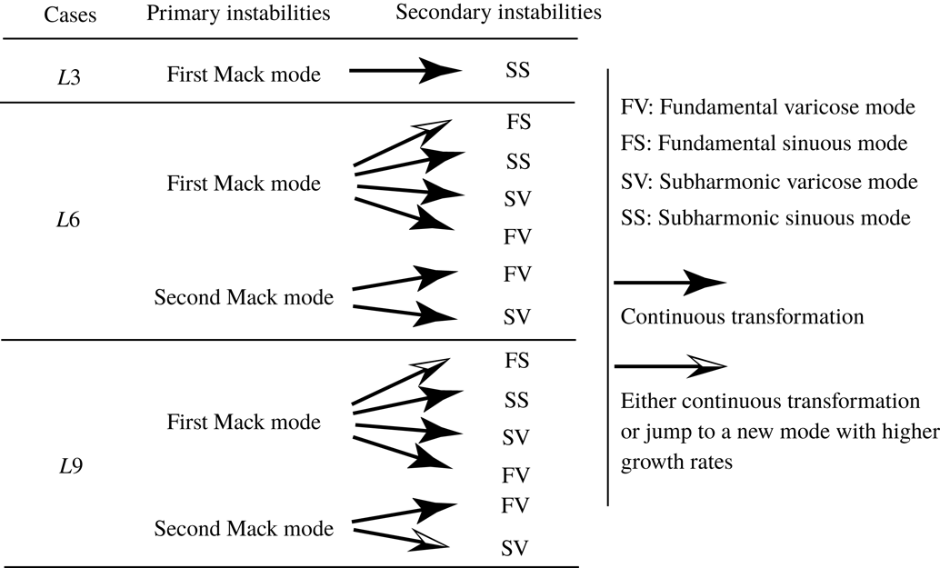
As the Görtler vortices grow, the boundary layer flow changes to form low- and high-speed streaks in the spanwise direction. When these streaks reach a certain amplitude, a high-frequency secondary instability may set in. Two distinct types of secondary instabilities, i.e. a varicose (symmetric) mode and a sinuous (antisymmetric) mode, have been extensively investigated. These two modes are known to be associated with inflectional streamwise velocity profiles in the wall-normal direction and the spanwise direction, respectively (Yu & Liu Reference Yu and Liu1994). Generally, the sinuous mode sets in earlier than the varicose mode and causes the streaks to meander. The varicose mode may become dominant further downstream (where the streaks become stronger) and develop horseshoe/hairpin structures. The secondary instability of the Görtler instability has also received considerable attention. Swearingen & Blackwelder (Reference Swearingen and Blackwelder1987) successfully visualized both the varicose and sinuous modes in experiments, and took detailed measurements of the fluctuations. They proposed that the spanwise shear plays a more prominent role in the transition to turbulence than the vertical shear. Their results were confirmed by Liu & Domaradzki (Reference Liu and Domaradzki1993) through a series of temporal numerical simulations. Li & Malik (Reference Li and Malik1995) found that the relative significance of these two secondary-instability modes depends upon the vortex wavelengths, i.e. short-wavelength vortices exhibit a stronger tendency towards the sinuous mode and long-wavelength vortices tend towards the varicose mode. Schrader, Brandt & Zaki (Reference Schrader, Brandt and Zaki2011) performed a spatial direct numerical simulation (DNS) of the boundary layer transition caused by Görtler vortices. Under broadband free stream disturbances which are represented by continuous spectra, they identified both varicose and sinuous instabilities in a single simulation. Sescu et al. (Reference Sescu, Sassanis, Haywood and Visbal2015) calculated the nonlinear evolution of the roughness-induced Görtler vortices, and used stability analysis to demonstrate that the varicose mode is most dangerous. By seeding unsteady disturbances via blowing and suction at locations where Görtler vortices have saturated, Souza (Reference Souza2017) found that sinuous modes appear first and dominate the transition process. Xu et al. (Reference Xu, Zhang and Wu2017) showed that sinuous modes are dominant for Görtler vortices excited by free stream turbulence.
Secondary instabilities of Görtler vortices in incompressible boundary layers have been studied extensively, but their hypersonic counterpart is not well understood. Wang & Zhong (Reference Wang and Zhong2001) simulated the evolution of nonlinear Görtler vortices in a Mach 15 curved-wall boundary layer and studied the secondary instability using bi-global analysis. They identified both varicose and sinuous modes, although both were linearly stable over the whole simulation region, and showed that the varicose mode is more unstable than the sinuous mode. In a Mach 6 study by Li et al. (Reference Li, Choudhari, Chang, Wu and Greene2010a ), however, the most dangerous mode was demonstrated to be the sinuous mode. Ren & Fu (Reference Ren and Fu2015a ) studied the nonlinear evolution and secondary instabilities of Görtler vortices at various Mach numbers with nonlinear parabolized stability equations and bi-global analysis. They showed that, in contrast to the incompressible case, the sinuous mode becomes the most dangerous at Mach numbers greater than 3, regardless of the spanwise wavelength.
The stability analyses mentioned above were performed only for ‘clear’ flows, in which the Görtler vortices are dominated by a single wavenumber or wavelength. However, under certain conditions, vortex generators not only excite the primary Görtler vortex with a wavelength equal to the spacing of the vortex generators, but also trigger the first harmonic with a comparable amplitude. Moreover, if the harmonic happens to be linearly unstable (which is quite possible as the range of unstable wavenumbers of Görtler vortices is broad), then the harmonic can grow and induce secondary streaks between the primary streaks. In fact, large-amplitude harmonic or secondary streaks have been reported in previous studies on incompressible flows. Souza et al. (Reference Souza, Mendonca, Medeiros and Kloker2004) utilized blowing and suction to excite Görtler vortices. They showed that, for large imposed wavelengths, the first harmonic can be generated and may even become the dominant mode downstream. Sescu et al. (Reference Sescu, Sassanis, Haywood and Visbal2015) numerically simulated the evolution of Görtler vortices triggered by roughness with various shapes, heights and diameters. They found that the roughness with the smallest diameter triggered Görtler vortices with double the wavenumber. In a series of wind-tunnel experiments, Mitsudharmadi and co-workers (Mitsudharmadi, Winoto & Shah Reference Mitsudharmadi, Winoto and Shah2005, Reference Mitsudharmadi, Winoto and Shah2006; Winoto et al.
Reference Winoto, Shah and Mitsudharmadi2008) excited Görtler vortices using distributed vertical wires. At the largest spanwise spacing of the wires, secondary streaks emerged between the primary streaks. They called this the splitting of Görtler vortices, and attributed it to the Eckhaus instability (Guo & Finlay Reference Guo and Finlay1991). Experiments on the transition of Görtler vortices were recently conducted in a Mach 6.5 wind tunnel at Peking University (personal communication) over a concave wall with a unit Reynolds number (
 $4\times 10^{6}~\text{m}^{-1}$
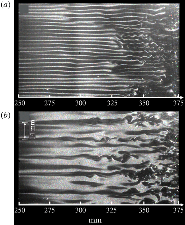
). The Görtler vortices were excited by a series of distributed roughness elements (small cylinders of height 0.6 mm and diameter 2 mm). The spacing of the roughness elements was 3 and 14 mm, respectively. Figure 1 shows the top view of the flow structures obtained by a CO
$4\times 10^{6}~\text{m}^{-1}$
). The Görtler vortices were excited by a series of distributed roughness elements (small cylinders of height 0.6 mm and diameter 2 mm). The spacing of the roughness elements was 3 and 14 mm, respectively. Figure 1 shows the top view of the flow structures obtained by a CO
 $_{2}$
Rayleigh-scattering technique. For the 3 mm case, the sinuous instability of the streaks is obvious. For the 14 mm case, however, the flow pattern is much more complex, and secondary streaks with a wavelength of 7 mm can be clearly observed. Furthermore, secondary streaks may also be relevant in the study of Xu et al. (Reference Xu, Zhang and Wu2017), who demonstrated the dominance of the harmonic for high-frequency free stream disturbances. For some phases of the flow fields in their study, secondary streaks may be present. It is expected that these secondary streaks would significantly change the flow profiles. However, the corresponding stability characteristics remain unknown.
$_{2}$
Rayleigh-scattering technique. For the 3 mm case, the sinuous instability of the streaks is obvious. For the 14 mm case, however, the flow pattern is much more complex, and secondary streaks with a wavelength of 7 mm can be clearly observed. Furthermore, secondary streaks may also be relevant in the study of Xu et al. (Reference Xu, Zhang and Wu2017), who demonstrated the dominance of the harmonic for high-frequency free stream disturbances. For some phases of the flow fields in their study, secondary streaks may be present. It is expected that these secondary streaks would significantly change the flow profiles. However, the corresponding stability characteristics remain unknown.
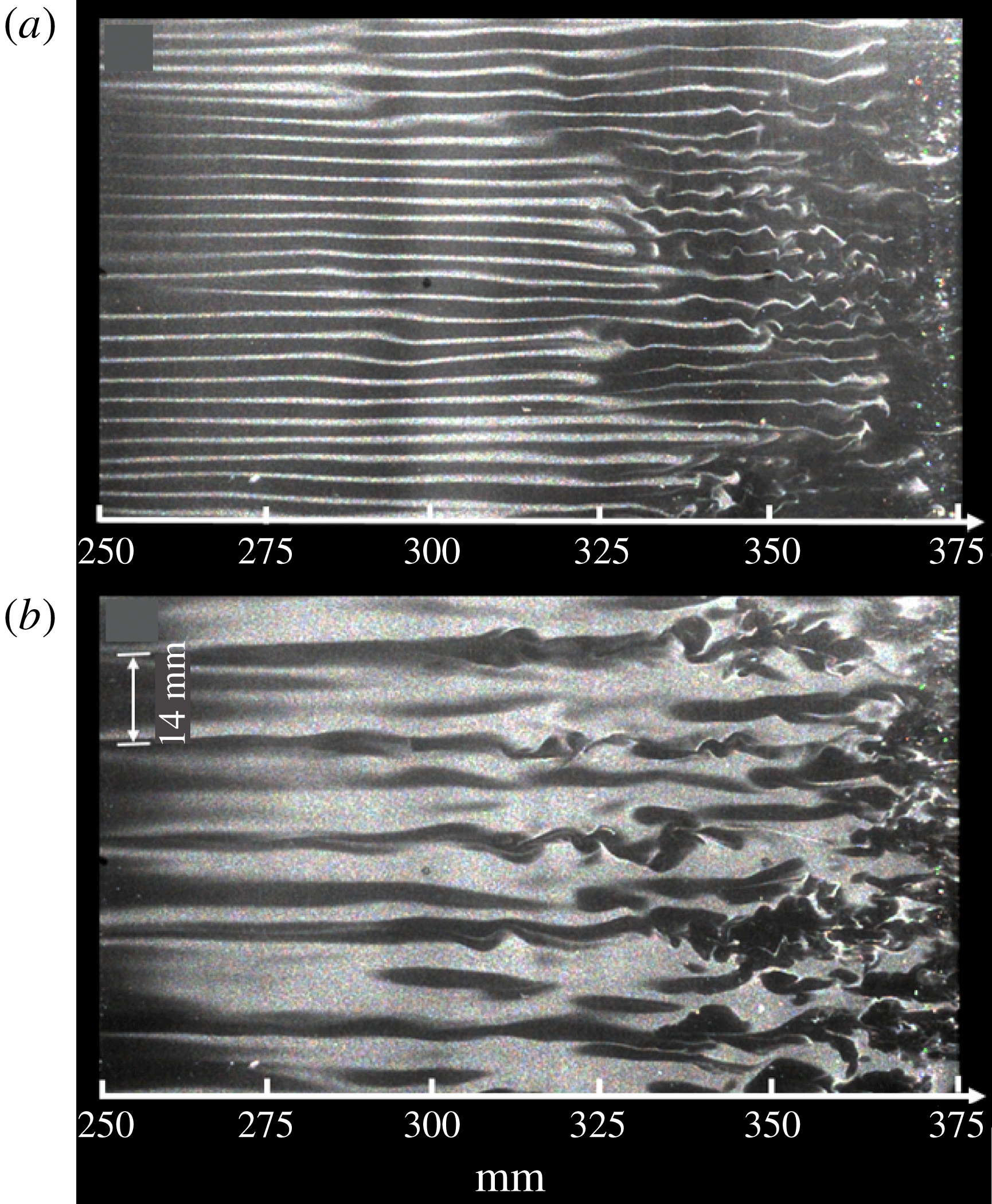
Figure 1. Single-shot spanwise images for a concave wall with roughness elements showing the emergence of streaks. The spacing of the roughness elements is 3 mm (a) and 14 mm (b).
In this study, we numerically excited Görtler vortices with various wavelengths in a hypersonic boundary layer by blowing and suction. The results described in this paper demonstrate that, for cases with large blowing and suction wavelengths, secondary streaks are likely to appear. The stability characteristics of the Görtler vortices with secondary streaks are analysed in detail for the first time. The secondary streaks significantly affect the stability of the boundary layer. Furthermore, we emphasize the importance of the transformation processes from primary instabilities to secondary instabilities, whereas previous studies have mostly focused on the secondary instabilities.
The rest of this article is organized as follows. In the next section, we present the model and numerical settings, and describe the mean flow characteristics. In § 3, we briefly introduce the linear stability analysis and energy analysis applied to the undisturbed mean flow as well as the streak flow field. In § 4, detailed DNS results and the stability theory results are presented. Finally, the outcomes of this study are summarized in § 5.
2 Model and numerical settings
2.1 Numerical tools
The model is sketched in figure 2. The flow conditions correspond to a free stream Mach number of 6.5, free stream pressure (
 $p_{e}$
) of 570 Pa, free stream temperature (
$p_{e}$
) of 570 Pa, free stream temperature (
 $T_{e}$
) of 53 K and unit Reynolds number (
$T_{e}$
) of 53 K and unit Reynolds number (
 $Re_{\infty }$
) of
$Re_{\infty }$
) of
 $9.0\times 10^{6}~\text{m}^{-1}$
. This model consists of a sharp flat plate and a 295 mm-long flared afterbody located 80 mm downstream from the leading edge. The flared body is generated by a circular curve with a radius (
$9.0\times 10^{6}~\text{m}^{-1}$
. This model consists of a sharp flat plate and a 295 mm-long flared afterbody located 80 mm downstream from the leading edge. The flared body is generated by a circular curve with a radius (
 $R$
) of 1.6 m. Thus, the global streamwise curvature,
$R$
) of 1.6 m. Thus, the global streamwise curvature,
 $K\equiv -Re_{\infty }R$
(Ren & Fu Reference Ren and Fu2015a
), is
$K\equiv -Re_{\infty }R$
(Ren & Fu Reference Ren and Fu2015a
), is
 $-6.2\times 10^{-8}$
. The region of interest is
$-6.2\times 10^{-8}$
. The region of interest is
 $x\in [80,350]~\text{mm}$
, resulting in
$x\in [80,350]~\text{mm}$
, resulting in
 $Re\equiv \sqrt{Re_{\infty }x}\in [848,1773]$
and a Görtler number
$Re\equiv \sqrt{Re_{\infty }x}\in [848,1773]$
and a Görtler number
 $G=Re\sqrt{\unicode[STIX]{x1D6FF}_{x}/R}\in [6.5,19.7]$
. Here,
$G=Re\sqrt{\unicode[STIX]{x1D6FF}_{x}/R}\in [6.5,19.7]$
. Here,
 $\unicode[STIX]{x1D6FF}_{x}=\sqrt{x/Re_{\infty }}$
denotes the boundary layer length scale. This range of Görtler number indicates that a local stability analysis is applicable (Bottaro & Luchini Reference Bottaro and Luchini1999). Qualitatively similar models have been used in supersonic experiments (Wang, Wang & Zhao Reference Wang, Wang and Zhao2018) and hypersonic experiments (de Luca et al.
Reference de Luca, Cardone, de la Chevalerie and Fonteneau1993). Here, the curved plane has been designed so that the Görtler instability can be easily observed while avoiding reversed flow.
$\unicode[STIX]{x1D6FF}_{x}=\sqrt{x/Re_{\infty }}$
denotes the boundary layer length scale. This range of Görtler number indicates that a local stability analysis is applicable (Bottaro & Luchini Reference Bottaro and Luchini1999). Qualitatively similar models have been used in supersonic experiments (Wang, Wang & Zhao Reference Wang, Wang and Zhao2018) and hypersonic experiments (de Luca et al.
Reference de Luca, Cardone, de la Chevalerie and Fonteneau1993). Here, the curved plane has been designed so that the Görtler instability can be easily observed while avoiding reversed flow.
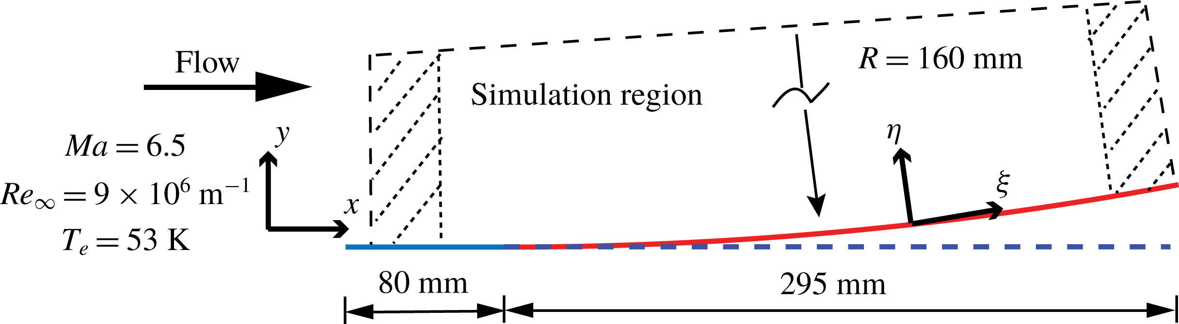
Figure 2. Sketch of the concave wall and the body-oriented coordinates.
The simulation starts from
 $x=10~\text{mm}$
, where a similarity solution is forced. The leading-edge shock effect is negligible because it is weak and far away from the vortices. A buffer zone near the outflow boundary is defined in which all disturbances gradually damp down to zero. Another buffer domain, located near the inflow boundary, is also implemented. These two buffer regions are used to avoid disturbances from reflections. No-slip and adiabatic conditions are prescribed at the wall. The wall-normal velocity component at the wall is specified in the blowing and suction strip regions, where the disturbances are introduced. The function used for the wall-normal velocity at the disturbance generator strip is
$x=10~\text{mm}$
, where a similarity solution is forced. The leading-edge shock effect is negligible because it is weak and far away from the vortices. A buffer zone near the outflow boundary is defined in which all disturbances gradually damp down to zero. Another buffer domain, located near the inflow boundary, is also implemented. These two buffer regions are used to avoid disturbances from reflections. No-slip and adiabatic conditions are prescribed at the wall. The wall-normal velocity component at the wall is specified in the blowing and suction strip regions, where the disturbances are introduced. The function used for the wall-normal velocity at the disturbance generator strip is
 $$\begin{eqnarray}\displaystyle v_{bs}(x,0,z,t)={\mathcal{A}}\sin ^{3}\left(\unicode[STIX]{x03C0}\frac{x-x_{1}}{x_{2}-x_{1}}\right)\cos (\unicode[STIX]{x1D6FD}z),\quad x_{1}\leqslant x\leqslant x_{2}, & & \displaystyle\end{eqnarray}$$
where
 ${\mathcal{A}}$
is a real constant chosen to set the amplitude of the disturbance. The variables
${\mathcal{A}}$
is a real constant chosen to set the amplitude of the disturbance. The variables
 $x_{1}$
and
$x_{1}$
and
 $x_{2}$
indicate the boundaries of the strip. The same function was used by Rogenski, Souza & Floryan (Reference Rogenski, Souza and Floryan2016) and Souza (Reference Souza2017).
$x_{2}$
indicate the boundaries of the strip. The same function was used by Rogenski, Souza & Floryan (Reference Rogenski, Souza and Floryan2016) and Souza (Reference Souza2017).
In this paper, we consider three different blowing–suction spanwise wavelengths, i.e. 3, 6 and 9 mm, and study the transition process for each case. Thus, the corresponding wavelength parameters,
 $\unicode[STIX]{x1D6EC}\equiv Re_{\infty }\unicode[STIX]{x1D706}_{z}\sqrt{\unicode[STIX]{x1D706}_{z}/R}$
, are 1170, 2340 and 3507, respectively. For simplicity, these three cases are hereafter denoted by
$\unicode[STIX]{x1D6EC}\equiv Re_{\infty }\unicode[STIX]{x1D706}_{z}\sqrt{\unicode[STIX]{x1D706}_{z}/R}$
, are 1170, 2340 and 3507, respectively. For simplicity, these three cases are hereafter denoted by
 $L3$
,
$L3$
,
 $L6$
and
$L6$
and
 $L9$
, respectively. The main blowing–suction region is located between 56.5 and 62.6 mm in the flat-plate region. A large initial amplitude, 15 % of the free stream velocity, is chosen to ensure there is an earlier saturation stage. Random fluctuations of 2 % are seeded downstream via a secondary blowing–suction strip
$L9$
, respectively. The main blowing–suction region is located between 56.5 and 62.6 mm in the flat-plate region. A large initial amplitude, 15 % of the free stream velocity, is chosen to ensure there is an earlier saturation stage. Random fluctuations of 2 % are seeded downstream via a secondary blowing–suction strip
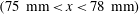 $(75~\text{mm}<x<78~\text{mm})$
to trigger the transition. Note that the upward/downward flow brings low-/high-speed fluid, inducing a velocity deficit/increase in the low-/high-speed region. Therefore, low-speed/high-temperature streaks should appear in the blowing regions (
$(75~\text{mm}<x<78~\text{mm})$
to trigger the transition. Note that the upward/downward flow brings low-/high-speed fluid, inducing a velocity deficit/increase in the low-/high-speed region. Therefore, low-speed/high-temperature streaks should appear in the blowing regions (
 $v_{bs}>0$
), whereas high-speed/low-temperature streaks are expected in the suction regions (
$v_{bs}>0$
), whereas high-speed/low-temperature streaks are expected in the suction regions (
 $v_{bs}<0$
).
$v_{bs}<0$
).
The parallel computational fluid dynamics software OPENCFD, developed by Li, Fu & Ma (Reference Li, Fu and Ma2008), was used for the DNS. Jacobian-transformed compressible Navier–Stokes equations in curved coordinates are solved numerically using high-order finite-difference methods. Convection terms are subjected to Steger–Warming splitting and discretized with a seventh-order weighted essentially non-oscillatory scheme, whereas viscous terms are discretized with an eighth-order centred finite-difference scheme. A third-order total variation diminishing-type Runge–Kutta method is used for the time stepping. Validation of the code can be found in a series of papers (Li et al. Reference Li, Fu and Ma2008; Liang et al. Reference Liang, Li, Fu and Ma2010; Li, Fu & Ma Reference Li, Fu and Ma2010b ).
The width of the simulation region is chosen to cover an even number of blowing–suction wavelengths in order to account for both fundamental and subharmonic disturbances. For
 $L3$
and
$L3$
and
 $L9$
, the width is 18 mm, whereas for
$L9$
, the width is 18 mm, whereas for
 $L6$
it is 24 mm. The physical domain is resolved by
$L6$
it is 24 mm. The physical domain is resolved by
 $1000\times 201\times 150$
grid points in the streamwise, wall-normal and spanwise directions, respectively, giving a total of 30 million points. The resolution is
$1000\times 201\times 150$
grid points in the streamwise, wall-normal and spanwise directions, respectively, giving a total of 30 million points. The resolution is
 $\unicode[STIX]{x0394}x^{+}=6.0$
,
$\unicode[STIX]{x0394}x^{+}=6.0$
,
 $\unicode[STIX]{x0394}y_{min}^{+}=0.6$
,
$\unicode[STIX]{x0394}y_{min}^{+}=0.6$
,
 $\unicode[STIX]{x0394}z^{+}=2.4$
for cases
$\unicode[STIX]{x0394}z^{+}=2.4$
for cases
 $L3$
and
$L3$
and
 $L9$
, and
$L9$
, and
 $\unicode[STIX]{x0394}z^{+}=3.2$
for
$\unicode[STIX]{x0394}z^{+}=3.2$
for
 $L6$
. The solution was tested by changing the number of grid points and it was found to be grid-independent.
$L6$
. The solution was tested by changing the number of grid points and it was found to be grid-independent.
2.2 Mean flow field
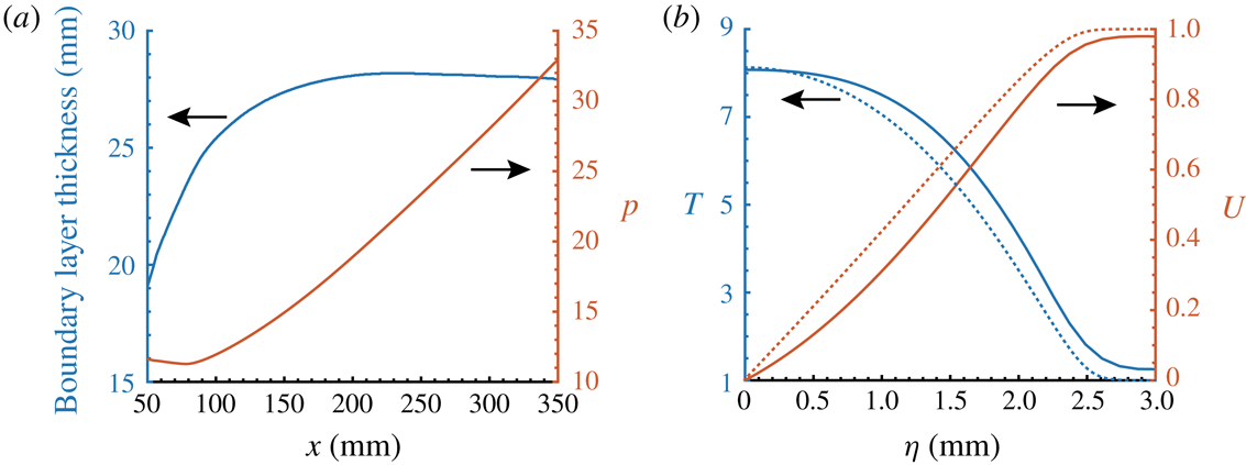
Figure 3(a) shows the development of the boundary layer thickness and wall pressure in the streamwise direction. The edge of the boundary layer is determined by the point at which the gradient of the streamwise velocity falls below a small constant. It can be seen that the curvature of the concave surface induces a significant pressure increase. As a result, the boundary layer thickness increases very slowly, and even decreases over the curved wall. This adverse pressure gradient also affects the mean flow profiles in at least two aspects, as shown in figure 3(b). First, there is a weak inflection point in the streamwise velocity, which is absent in the similarity solutions. Second, the temperature and velocity do not exactly take the free stream values at the boundary layer edge. In fact, a large inviscid region beyond the boundary layer is required for the main variables to recover the free stream values.
3 Stability analysis
3.1 Stability theory
In this paper, we consider the stability characteristics along the wall-normal direction (
 $\unicode[STIX]{x1D702}$
, one-dimensional LST) or in a
$\unicode[STIX]{x1D702}$
, one-dimensional LST) or in a
 $\unicode[STIX]{x1D702}$
–
$\unicode[STIX]{x1D702}$
–
 $z$
cross-section (two-dimensional LST or bi-global). The respective decompositions of the flow field are given by
$z$
cross-section (two-dimensional LST or bi-global). The respective decompositions of the flow field are given by
 $$\begin{eqnarray}\displaystyle q(\unicode[STIX]{x1D709},\unicode[STIX]{x1D702},z,t)=\bar{q}(\unicode[STIX]{x1D702})+q^{\prime }(\unicode[STIX]{x1D702})=\bar{q}(\unicode[STIX]{x1D702})+\hat{q}(\unicode[STIX]{x1D702})\exp (\text{i}\unicode[STIX]{x1D6FC}\unicode[STIX]{x1D709}+\text{i}\unicode[STIX]{x1D6FD}z-\text{i}\unicode[STIX]{x1D714}t)+\text{c.c.} & & \displaystyle\end{eqnarray}$$
and
 $$\begin{eqnarray}\displaystyle q(\unicode[STIX]{x1D709},\unicode[STIX]{x1D702},z,t)=\bar{q}(\unicode[STIX]{x1D702},z)+q^{\prime }(\unicode[STIX]{x1D702},z)=\bar{q}(\unicode[STIX]{x1D702},z)+\hat{q}(\unicode[STIX]{x1D702},z)\exp (\text{i}\unicode[STIX]{x1D6FC}\unicode[STIX]{x1D709}-\text{i}\unicode[STIX]{x1D714}t)+\text{c.c.}, & & \displaystyle\end{eqnarray}$$
where
 $q=(\unicode[STIX]{x1D70C},u,v,w,T)$
,
$q=(\unicode[STIX]{x1D70C},u,v,w,T)$
,
 $\bar{q}$
denotes the basic states,
$\bar{q}$
denotes the basic states,
 $q^{\prime }$
denotes the disturbances,
$q^{\prime }$
denotes the disturbances,
 $\hat{q}$
is the shape function of the disturbances,
$\hat{q}$
is the shape function of the disturbances,
 $\unicode[STIX]{x1D6FC}$
and
$\unicode[STIX]{x1D6FC}$
and
 $\unicode[STIX]{x1D6FD}$
represent the streamwise and spanwise wavenumbers, respectively, with corresponding wavelengths denoted by
$\unicode[STIX]{x1D6FD}$
represent the streamwise and spanwise wavenumbers, respectively, with corresponding wavelengths denoted by
 $\unicode[STIX]{x1D706}$
in the streamwise direction and
$\unicode[STIX]{x1D706}$
in the streamwise direction and
 $\unicode[STIX]{x1D706}_{z}$
in the spanwise direction and
$\unicode[STIX]{x1D706}_{z}$
in the spanwise direction and
 $\unicode[STIX]{x1D714}$
is the angular frequency with corresponding dimensional frequency denoted by
$\unicode[STIX]{x1D714}$
is the angular frequency with corresponding dimensional frequency denoted by
 $f$
. After substituting the above decompositions into the Navier–Stokes equations, subtracting the basic states and neglecting the non-parallel and nonlinear terms, one obtains the eigenvalue problems
$f$
. After substituting the above decompositions into the Navier–Stokes equations, subtracting the basic states and neglecting the non-parallel and nonlinear terms, one obtains the eigenvalue problems
 $$\begin{eqnarray}\displaystyle {\mathcal{L}}_{1}(\unicode[STIX]{x1D702},\unicode[STIX]{x1D6FC},\unicode[STIX]{x1D6FD},\unicode[STIX]{x1D714})\hat{q}(\unicode[STIX]{x1D702})=0 & & \displaystyle\end{eqnarray}$$
for one-dimensional LST and
 $$\begin{eqnarray}\displaystyle {\mathcal{L}}_{2}(\unicode[STIX]{x1D702},z,\unicode[STIX]{x1D6FC},\unicode[STIX]{x1D6FD},\unicode[STIX]{x1D714})\hat{q}(\unicode[STIX]{x1D702},z)=0 & & \displaystyle\end{eqnarray}$$
for two-dimensional LST. Here,
 ${\mathcal{L}}$
is a linear operator that has been described in the literature (e.g. Malik Reference Malik1990). The boundary conditions are
${\mathcal{L}}$
is a linear operator that has been described in the literature (e.g. Malik Reference Malik1990). The boundary conditions are
 $$\begin{eqnarray}\hat{u} =\hat{v}={\hat{w}}=\frac{\unicode[STIX]{x2202}\hat{T}}{\unicode[STIX]{x2202}\unicode[STIX]{x1D702}}=0\quad \text{at }\unicode[STIX]{x1D702}=0\quad \text{and}\quad \hat{u} =\hat{v}={\hat{w}}=\hat{T}=0\quad \text{at }\unicode[STIX]{x1D702}\rightarrow \infty .\end{eqnarray}$$
Note that the Neumann boundary condition for temperature perturbations is used for consistency with the DNS boundary conditions. Numerical experiments show that using a Dirichlet boundary condition for temperature produces similar results. For one-dimensional LST, the spatial analysis is applied by specifying
 $\unicode[STIX]{x1D714}$
and determining the eigenvalue
$\unicode[STIX]{x1D714}$
and determining the eigenvalue
 $\unicode[STIX]{x1D6FC}$
. For two-dimensional LST, a temporal analysis is considered for the sake of simplicity, where
$\unicode[STIX]{x1D6FC}$
. For two-dimensional LST, a temporal analysis is considered for the sake of simplicity, where
 $\unicode[STIX]{x1D6FC}$
is given and
$\unicode[STIX]{x1D6FC}$
is given and
 $\unicode[STIX]{x1D714}$
is to be determined. The temporal growth rate can then be converted into the spatial growth rate via the group-velocity approach (Gaster Reference Gaster1962) if necessary. The linear operator is discretized using the Chebyshev and Fourier collocation methods in the
$\unicode[STIX]{x1D714}$
is to be determined. The temporal growth rate can then be converted into the spatial growth rate via the group-velocity approach (Gaster Reference Gaster1962) if necessary. The linear operator is discretized using the Chebyshev and Fourier collocation methods in the
 $\unicode[STIX]{x1D702}$
and
$\unicode[STIX]{x1D702}$
and
 $z$
directions, respectively. For the bi-global analysis, the discretized
$z$
directions, respectively. For the bi-global analysis, the discretized
 ${\mathcal{L}}$
is a square matrix of size
${\mathcal{L}}$
is a square matrix of size
 $5N_{\unicode[STIX]{x1D702}}N_{z}\times 5N_{\unicode[STIX]{x1D702}}N_{z}$
, the eigenvalues of which can be determined using Arnoldi’s method.
$5N_{\unicode[STIX]{x1D702}}N_{z}\times 5N_{\unicode[STIX]{x1D702}}N_{z}$
, the eigenvalues of which can be determined using Arnoldi’s method.

Figure 3. Mean flow characteristics: (a) the boundary layer thickness and wall pressure; (b) normalized streamwise velocity and temperature at
 $x=250~\text{mm}$
. The dotted lines represent the similarity profiles.
$x=250~\text{mm}$
. The dotted lines represent the similarity profiles.

Figure 4. Contours of the constant amplification rate
 $-\unicode[STIX]{x1D6FC}_{i}$
(
$-\unicode[STIX]{x1D6FC}_{i}$
(
 $\text{mm}^{-1}$
) in the (
$\text{mm}^{-1}$
) in the (
 $x$
–
$x$
–
 $f$
) plane for planar disturbances (a) and in the (
$f$
) plane for planar disturbances (a) and in the (
 $\unicode[STIX]{x1D706}_{z}$
–
$\unicode[STIX]{x1D706}_{z}$
–
 $f$
) plane for three-dimensional waves at (b)
$f$
) plane for three-dimensional waves at (b)
 $x=228~\text{mm}$
and (c)
$x=228~\text{mm}$
and (c)
 $x=228~\text{mm}$
with the curvature turned off. All the plots have the same contour levels.
$x=228~\text{mm}$
with the curvature turned off. All the plots have the same contour levels.
Figure 4 displays the contours of the constant amplification rate for planar and three-dimensional disturbances. The unstable region in figure 4(a) is caused only by the second Mack-mode instability. The two-dimensional first Mack-mode instability is very weak and is not shown here. Figure 4(b) depicts the unstable regions of three-dimensional disturbances at
 $x=228~\text{mm}$
. The region located above
$x=228~\text{mm}$
. The region located above
 $f=100~\text{kHz}$
is associated with the second Mack-mode instability, which is more unstable for larger spanwise wavelengths. The first Mack-mode and Görtler instabilities lie in the low-frequency region and are highly dependent on the spanwise wavelengths. To distinguish these two instabilities, we turned off the curvature effect in the LST solver and display the unstable regions at the same location in figure 4(c). By comparing figure 4(b,c), one can easily see that the first Mack mode is centred around (10 mm, 50 kHz), whereas the Görtler instability lies in a triangle-like region with vertices at approximately (10 mm, 0 kHz), (1 mm, 0 kHz) and (1 mm, 150 kHz).
$f=100~\text{kHz}$
is associated with the second Mack-mode instability, which is more unstable for larger spanwise wavelengths. The first Mack-mode and Görtler instabilities lie in the low-frequency region and are highly dependent on the spanwise wavelengths. To distinguish these two instabilities, we turned off the curvature effect in the LST solver and display the unstable regions at the same location in figure 4(c). By comparing figure 4(b,c), one can easily see that the first Mack mode is centred around (10 mm, 50 kHz), whereas the Görtler instability lies in a triangle-like region with vertices at approximately (10 mm, 0 kHz), (1 mm, 0 kHz) and (1 mm, 150 kHz).
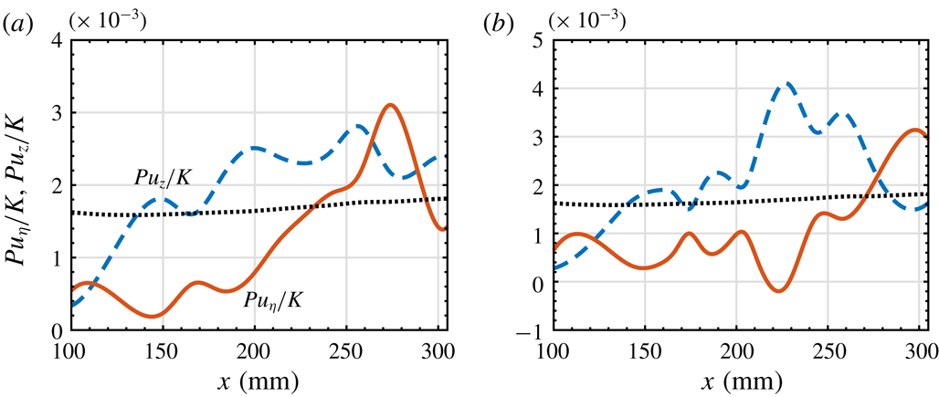
3.2 Energy analysis
Knowing the production terms associated with the local kinetic energy transfer provides further understanding of the mechanism for the instability modes. The local streamwise rate of change of the integrated kinetic energy is given by (Paredes, Choudhari & Li Reference Paredes, Choudhari and Li2017a )
 $$\begin{eqnarray}\displaystyle \frac{\unicode[STIX]{x2202}K(x)}{\unicode[STIX]{x2202}x}=P(x)-D(x), & & \displaystyle\end{eqnarray}$$
where
 $K$
is the kinetic energy of the disturbance, defined as
$K$
is the kinetic energy of the disturbance, defined as
 $$\begin{eqnarray}\displaystyle K(x)=\int _{z}\int _{\unicode[STIX]{x1D702}}\bar{\unicode[STIX]{x1D70C}}(\hat{u} \hat{u} ^{\ast }+\hat{v}\hat{v}^{\ast }+{\hat{w}}{\hat{w}}^{\ast })\,\text{d}\unicode[STIX]{x1D702}\,\text{d}z, & & \displaystyle\end{eqnarray}$$
in which the superscript * denotes the complex conjugate,
 $D$
is the viscous dissipation and
$D$
is the viscous dissipation and
 $P$
is the production. The two components of
$P$
is the production. The two components of
 $P$
that are of most interest are
$P$
that are of most interest are
 $$\begin{eqnarray}\displaystyle Pu_{\unicode[STIX]{x1D702}}=\int _{z}\int _{\unicode[STIX]{x1D702}}-\text{Re}(\hat{u} \hat{v}^{\ast })\bar{\unicode[STIX]{x1D70C}}\bar{u}_{\unicode[STIX]{x1D702}}\,\text{d}\unicode[STIX]{x1D702}\,\text{d}z\quad \text{and}\quad Pu_{z}=\int _{z}\int _{\unicode[STIX]{x1D702}}-\text{Re}(\hat{u} {\hat{w}}^{\ast })\bar{\unicode[STIX]{x1D70C}}\bar{u}_{z}\,\text{d}\unicode[STIX]{x1D702}\,\text{d}z.\qquad & & \displaystyle\end{eqnarray}$$
4 Numerical results
Prior to conducting the nonlinear simulations, DNS was performed with very low amplitudes to ensure that the linear regime was maintained throughout the entire computational domain. These simulations allow a direct comparison of the DNS results with LST. In figure 5(a), the downstream development of wall pressure disturbances (absolute values) is compared with that from LST for the most amplified second Mack-mode wave (
 $f=135~\text{kHz}$
). There is a good agreement between the DNS and LST data. The disturbance in the DNS grows slightly faster than that in the LST, which is likely due to non-parallel effects. Figure 5(b) displays the mode shapes of the second Mack-mode wave at
$f=135~\text{kHz}$
). There is a good agreement between the DNS and LST data. The disturbance in the DNS grows slightly faster than that in the LST, which is likely due to non-parallel effects. Figure 5(b) displays the mode shapes of the second Mack-mode wave at
 $x=220~\text{mm}$
based on DNS and LST data. Good agreement can again be observed, with slight differences likely to be caused by non-parallel effects.
$x=220~\text{mm}$
based on DNS and LST data. Good agreement can again be observed, with slight differences likely to be caused by non-parallel effects.
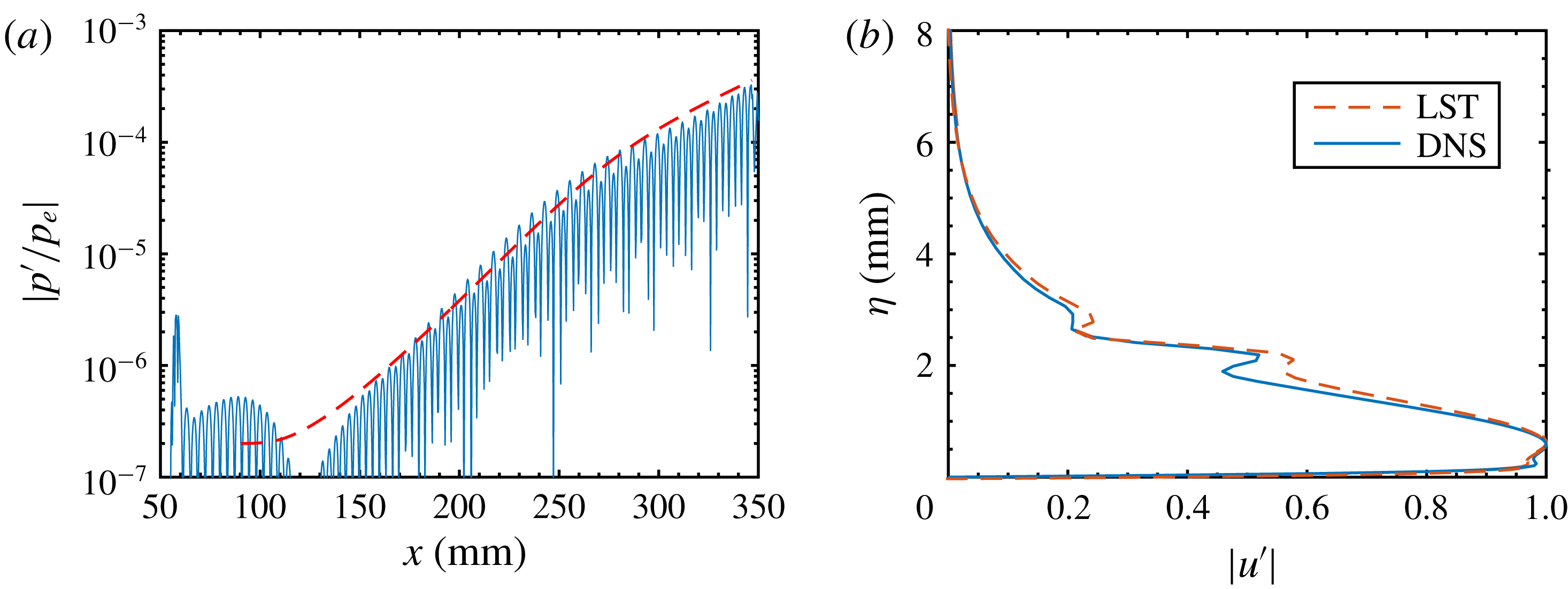
Figure 5. Comparison of LST (dashed lines) and DNS (solid lines) results of the most amplified second Mack-mode wave (
 $f=135~\text{kHz}$
). (a) Amplitude evolution of normalized wall pressure disturbances. (b) Streamwise velocity fluctuation at
$f=135~\text{kHz}$
). (a) Amplitude evolution of normalized wall pressure disturbances. (b) Streamwise velocity fluctuation at
 $x=300~\text{mm}$
.
$x=300~\text{mm}$
.
4.1 Visualizations
First, we display the temperature contours at various locations in the
 $x$
–
$x$
–
 $z$
and
$z$
and
 $z$
–
$z$
–
 $\unicode[STIX]{x1D702}$
planes. These contours mimic the experimental visualizations obtained from the Rayleigh scattering of CO
$\unicode[STIX]{x1D702}$
planes. These contours mimic the experimental visualizations obtained from the Rayleigh scattering of CO
 $_{2}$
for other problems (Auvity, Etz & Smits Reference Auvity, Etz and Smits2001; Zhang, Tang & Lee Reference Zhang, Tang and Lee2013). In experiments, CO
$_{2}$
for other problems (Auvity, Etz & Smits Reference Auvity, Etz and Smits2001; Zhang, Tang & Lee Reference Zhang, Tang and Lee2013). In experiments, CO
 $_{2}$
is injected upstream and undergoes phase changes across the boundary layer owing to large temperature variations. In the free stream, as the static temperature is low, the CO
$_{2}$
is injected upstream and undergoes phase changes across the boundary layer owing to large temperature variations. In the free stream, as the static temperature is low, the CO
 $_{2}$
condenses and forms nanometre-scale clusters. When the CO
$_{2}$
condenses and forms nanometre-scale clusters. When the CO
 $_{2}$
clusters become entrained in the boundary layer, the high temperature above the sublimation point causes the condensed particles to vaporize. The boundary layer is, therefore, imaged as a region of low-intensity Rayleigh signals, bounded by bright regions corresponding to the free stream fluid. In our numerical visualizations, the bright regions are occupied by fluid at temperatures below
$_{2}$
clusters become entrained in the boundary layer, the high temperature above the sublimation point causes the condensed particles to vaporize. The boundary layer is, therefore, imaged as a region of low-intensity Rayleigh signals, bounded by bright regions corresponding to the free stream fluid. In our numerical visualizations, the bright regions are occupied by fluid at temperatures below
 $2.7Te$
(or 143 K), which is close to the sublimation value of CO
$2.7Te$
(or 143 K), which is close to the sublimation value of CO
 $_{2}$
under a pressure of approximately 1 kPa.
$_{2}$
under a pressure of approximately 1 kPa.
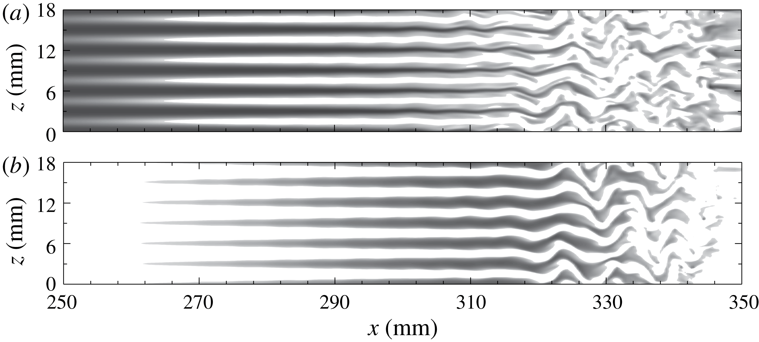
Figure 6. Snapshot of temperature contours at various distances from the wall for
 $L3$
: (a)
$L3$
: (a)
 $\unicode[STIX]{x1D702}=0.7~\text{mm}$
; (b)
$\unicode[STIX]{x1D702}=0.7~\text{mm}$
; (b)
 $\unicode[STIX]{x1D702}=2.75~\text{mm}$
. Regions with a temperature below
$\unicode[STIX]{x1D702}=2.75~\text{mm}$
. Regions with a temperature below
 $2.7T_{e}$
are not shown. A darker region represents a higher temperature.
$2.7T_{e}$
are not shown. A darker region represents a higher temperature.
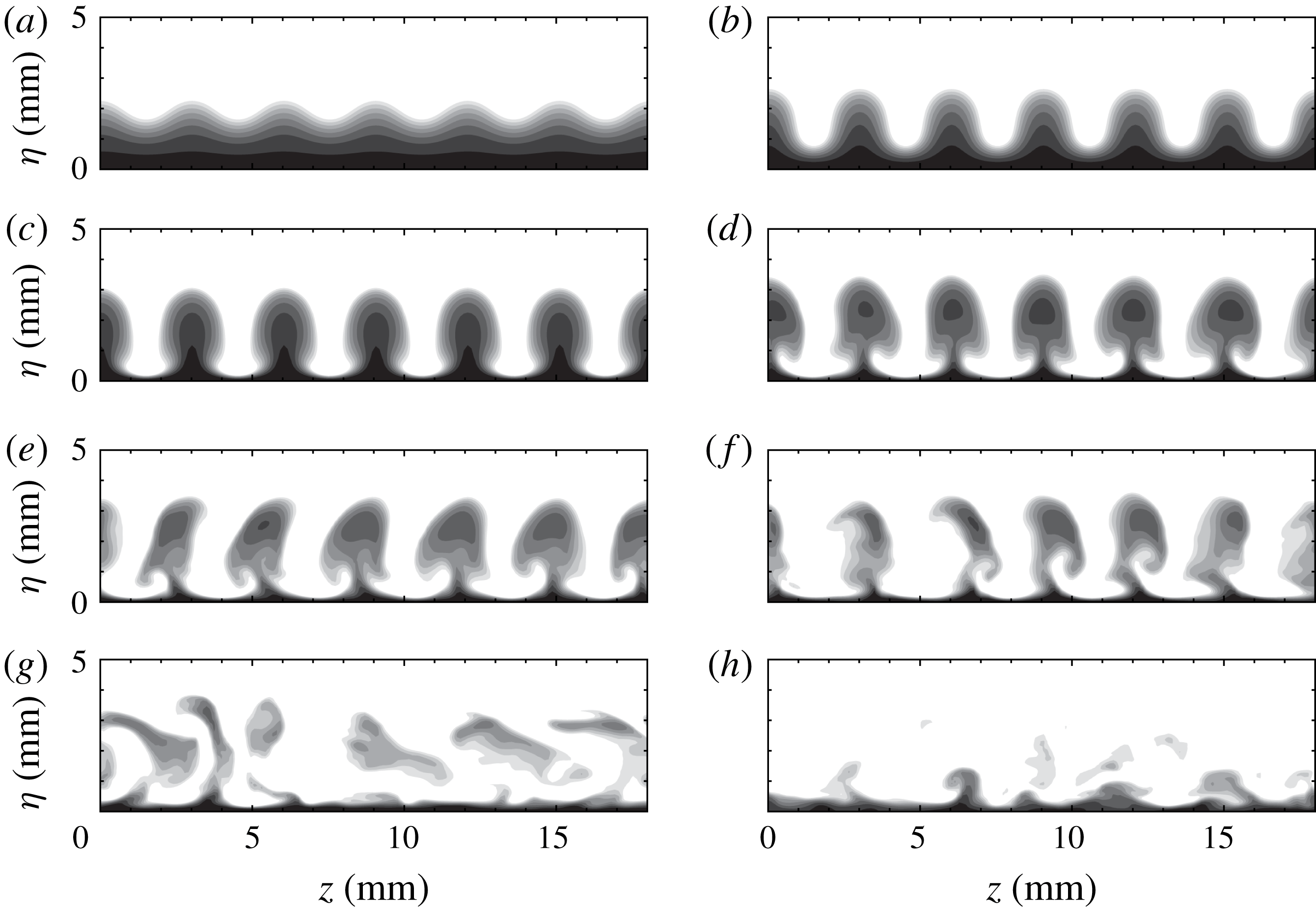
Figure 7. Snapshot of temperature contours at various streamwise locations for
 $L3$
(see supplementary movie 1 available at https://doi.org/10.1017/jfm.2019.24): (a)
$L3$
(see supplementary movie 1 available at https://doi.org/10.1017/jfm.2019.24): (a)
 $x=197~\text{mm}$
; (b)
$x=197~\text{mm}$
; (b)
 $x=258~\text{mm}$
; (c)
$x=258~\text{mm}$
; (c)
 $x=292~\text{mm}$
; (d)
$x=292~\text{mm}$
; (d)
 $x=313~\text{mm}$
; (e)
$x=313~\text{mm}$
; (e)
 $x=319~\text{mm}$
; (f)
$x=319~\text{mm}$
; (f)
 $x=322~\text{mm}$
; (g)
$x=322~\text{mm}$
; (g)
 $x=332~\text{mm}$
; (h)
$x=332~\text{mm}$
; (h)
 $x=344~\text{mm}$
.
$x=344~\text{mm}$
.
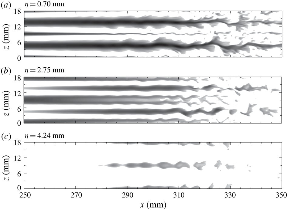
Figure 6 shows top views for
 $L3$
at two distances from the wall. The high-temperature streaks (dark regions) formed at the blowing positions, as expected, move upwards, and become larger downstream, as indicated by figure 6(b). These streaks remain straight over a long distance until
$L3$
at two distances from the wall. The high-temperature streaks (dark regions) formed at the blowing positions, as expected, move upwards, and become larger downstream, as indicated by figure 6(b). These streaks remain straight over a long distance until
 $x\approx 310~\text{mm}$
, at which point they start oscillating and soon break down. The meandering of streaks is likely to be caused by sinuous instabilities with a streamwise wavelength of approximately 9 mm.
$x\approx 310~\text{mm}$
, at which point they start oscillating and soon break down. The meandering of streaks is likely to be caused by sinuous instabilities with a streamwise wavelength of approximately 9 mm.
The end views in figure 7 show the detailed evolution of the streak structures. The vertical fluctuation initially induces wave profiles with the same period as the blowing and suction. These wave profiles develop into bell shapes at
 $x=258~\text{mm}$
, followed by mushroom structures at
$x=258~\text{mm}$
, followed by mushroom structures at
 $x=292~\text{mm}$
. Farther downstream, the symmetry of the structures soon breaks down as secondary instabilities set in at
$x=292~\text{mm}$
. Farther downstream, the symmetry of the structures soon breaks down as secondary instabilities set in at
 $x=313~\text{mm}$
. The oscillation of the streaks intensifies and eventually causes them to break down at
$x=313~\text{mm}$
. The oscillation of the streaks intensifies and eventually causes them to break down at
 $x=344~\text{mm}$
, as shown in figure 7(h).
$x=344~\text{mm}$
, as shown in figure 7(h).
Increasing the blowing–suction wavelength from 3 to 6 mm leads to significantly different results, as shown in figure 8. In contrast to expectations, strong high-temperature streaks appear downstream of the suction regions and are dominant in the near-wall region. We denote these as secondary streaks to distinguish them from the primary streaks aligned with the blowing regions. In the next section, we show that the secondary streaks are induced by the first harmonic of the primary Görtler vortices and are nonlinearly generated through large-amplitude blowing and suction. These secondary streaks broaden rapidly, with tiny structures developing on their sides, and then saturate and break down after
 $x\approx 310~\text{mm}$
. The primary streaks gradually disappear in the near-wall region and move upwards downstream. On top of the primary streaks, knotty structures develop and split into isolated parts, which appear to be associated with varicose modes.
$x\approx 310~\text{mm}$
. The primary streaks gradually disappear in the near-wall region and move upwards downstream. On top of the primary streaks, knotty structures develop and split into isolated parts, which appear to be associated with varicose modes.
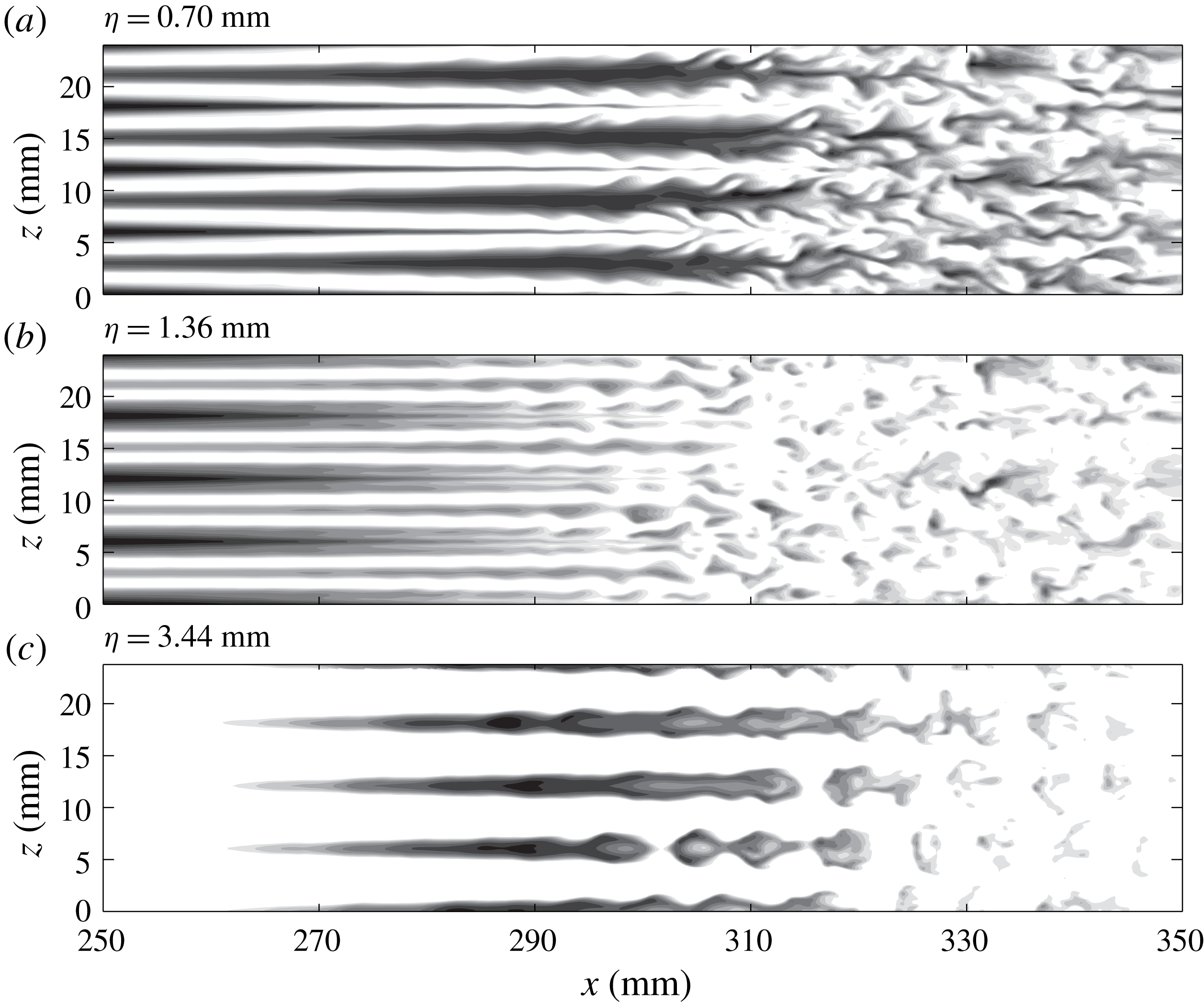
Figure 8. Snapshot of temperature contours at various distances from the wall for case
 $L6$
.
$L6$
.
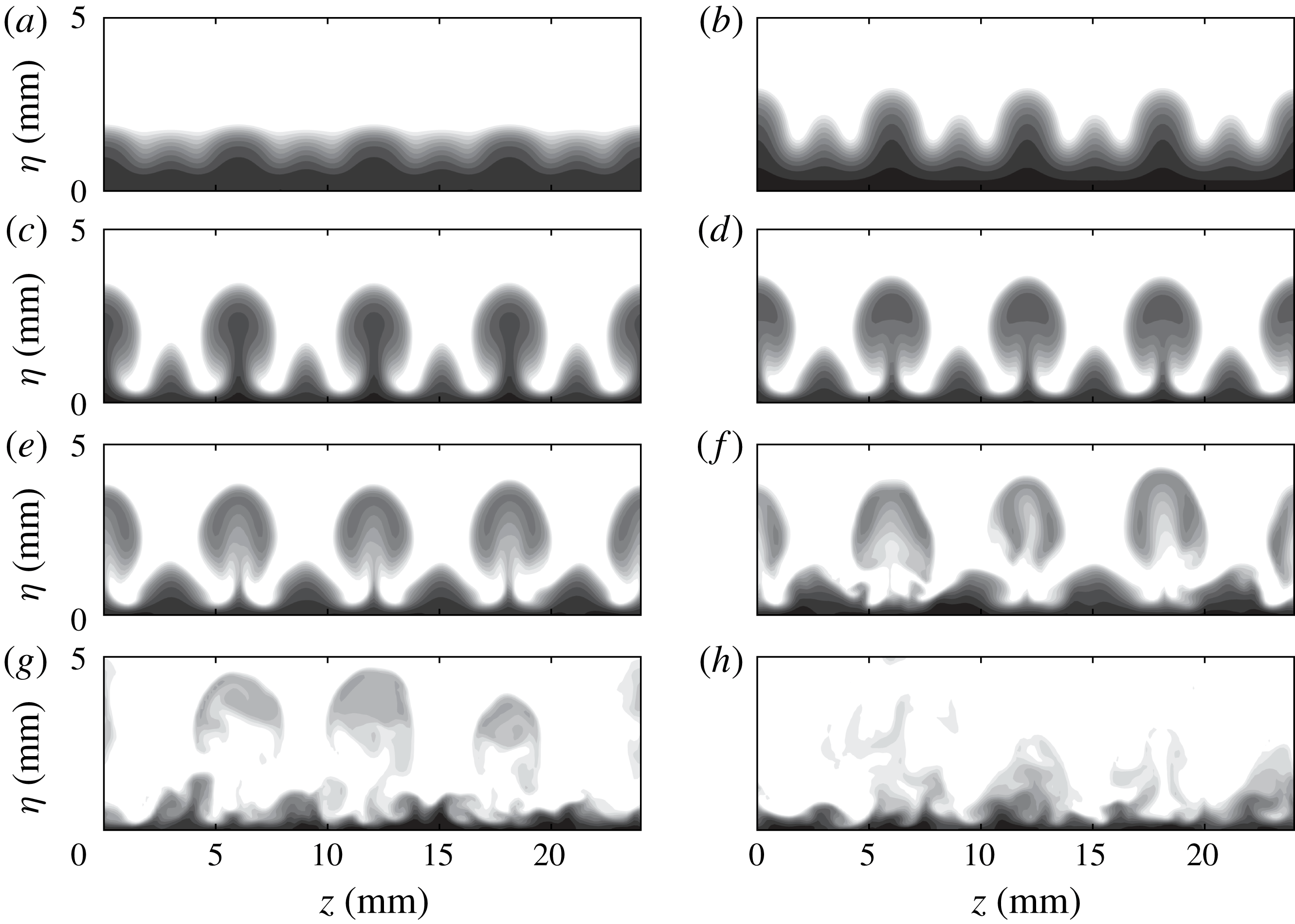
Figure 9. Snapshot of temperature contours at various streamwise locations for
 $L6$
(see movie 2): (a)
$L6$
(see movie 2): (a)
 $x=74.9~\text{mm}$
; (b)
$x=74.9~\text{mm}$
; (b)
 $x=197.1~\text{mm}$
; (c)
$x=197.1~\text{mm}$
; (c)
 $x=258.2~\text{mm}$
; (d)
$x=258.2~\text{mm}$
; (d)
 $x=273.4~\text{mm}$
; (e)
$x=273.4~\text{mm}$
; (e)
 $x=288.7~\text{mm}$
; (f)
$x=288.7~\text{mm}$
; (f)
 $x=304~\text{mm}$
; (g)
$x=304~\text{mm}$
; (g)
 $x=319.3~\text{mm}$
; (h)
$x=319.3~\text{mm}$
; (h)
 $x=334.5~\text{mm}$
.
$x=334.5~\text{mm}$
.
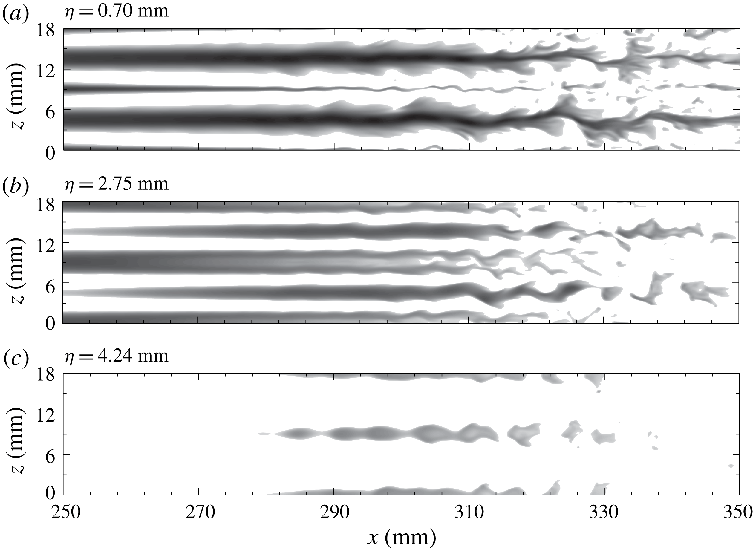
Figure 10. Temperature contours at various distances from the wall for
 $L9$
.
$L9$
.
Finally, we consider case
 $L9$
. Like
$L9$
. Like
 $L6$
, both primary and secondary streaks appear, with the former dominating the upper boundary layer and the latter the near-wall region, as shown in figure 10. Figure 10(a,c) clearly shows that the secondary streaks are susceptible to sinuous instabilities, while the primary streaks are subject to varicose instabilities. In contrast to
$L6$
, both primary and secondary streaks appear, with the former dominating the upper boundary layer and the latter the near-wall region, as shown in figure 10. Figure 10(a,c) clearly shows that the secondary streaks are susceptible to sinuous instabilities, while the primary streaks are subject to varicose instabilities. In contrast to
 $L6$
, the widths of the secondary streaks remain nearly constant before gradually decaying. More interestingly, the sinuous and varicose instabilities can coexist in the same plane, as shown in figure 10(b).
$L6$
, the widths of the secondary streaks remain nearly constant before gradually decaying. More interestingly, the sinuous and varicose instabilities can coexist in the same plane, as shown in figure 10(b).
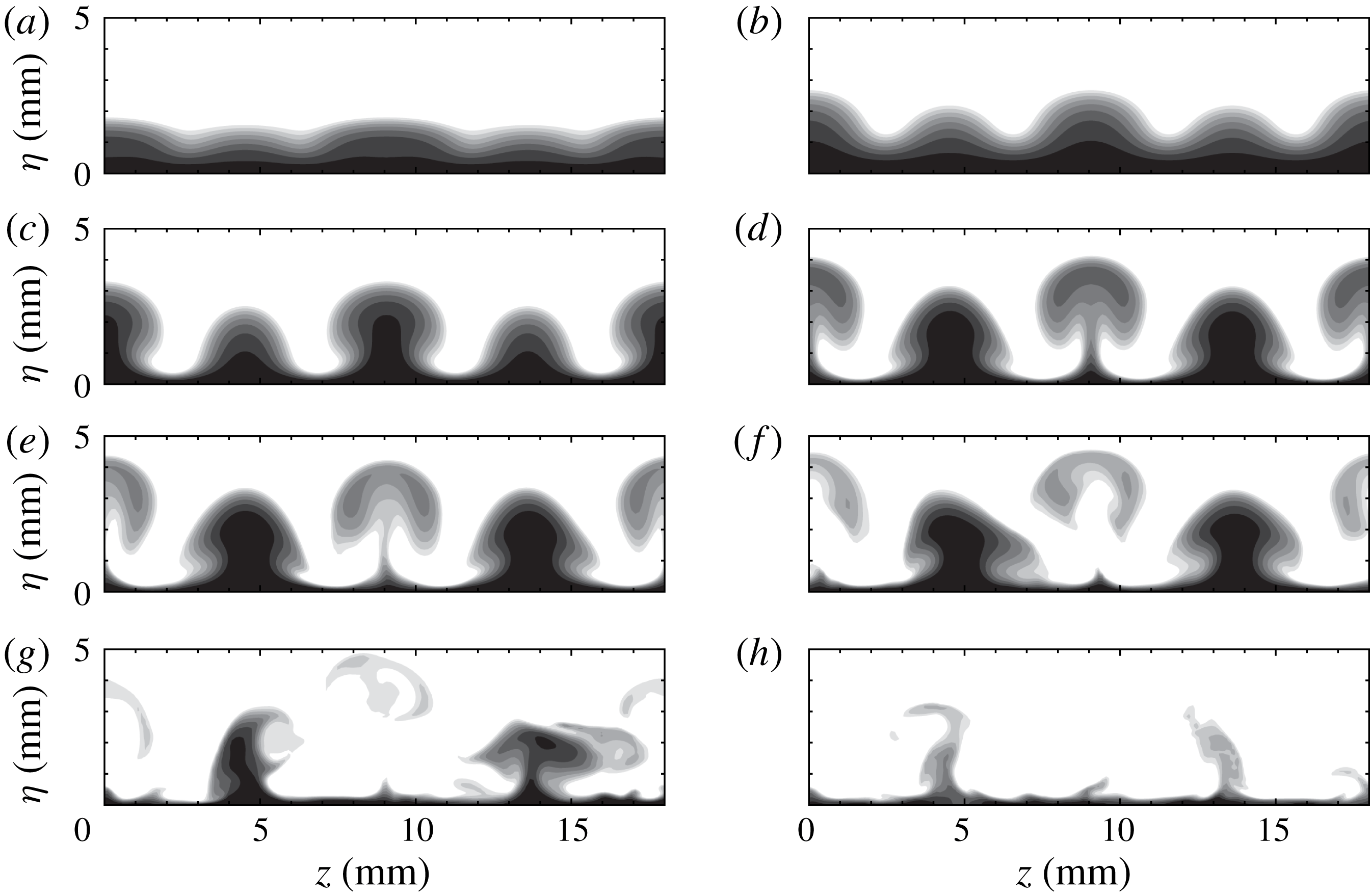
Figure 11. Snapshot of temperature contours at various streamwise locations for
 $L9$
(see movie 3): (a)
$L9$
(see movie 3): (a)
 $x=74.9~\text{mm}$
; (b)
$x=74.9~\text{mm}$
; (b)
 $x=166.5~\text{mm}$
; (c)
$x=166.5~\text{mm}$
; (c)
 $x=227.6~\text{mm}$
; (d)
$x=227.6~\text{mm}$
; (d)
 $x=273.4~\text{mm}$
; (e)
$x=273.4~\text{mm}$
; (e)
 $x=288.7~\text{mm}$
; (f)
$x=288.7~\text{mm}$
; (f)
 $x=304~\text{mm}$
; (g)
$x=304~\text{mm}$
; (g)
 $x=319.3~\text{mm}$
; (h)
$x=319.3~\text{mm}$
; (h)
 $x=346.8~\text{mm}$
.
$x=346.8~\text{mm}$
.
The end views of
 $L9$
exhibit some similarities to those of
$L9$
exhibit some similarities to those of
 $L6$
, as shown in figure 11. The initially excited wave profiles also contain two periodic waves. The primary waves develop into mushroom structures and soon break down. Triangle-like structures also evolve from the secondary waves and start to oscillate from
$L6$
, as shown in figure 11. The initially excited wave profiles also contain two periodic waves. The primary waves develop into mushroom structures and soon break down. Triangle-like structures also evolve from the secondary waves and start to oscillate from
 $x=288.7~\text{mm}$
. Consistent with the top view in figure 10(a), the secondary streaks are still visible at the end of the simulation domain.
$x=288.7~\text{mm}$
. Consistent with the top view in figure 10(a), the secondary streaks are still visible at the end of the simulation domain.
Figure 12 presents the time-averaged wall temperature variations relative to the laminar adiabatic values. This is similar to the temperature-sensitive painting visualization that is often used to detect temperature variations in hypersonic experiments (e.g. Chou et al.
Reference Chou, Ward, Letterman, Luersen, Borg and Schneider2011; Zhu et al.
Reference Zhu, Chen, Wu, Chen, Lee and Gadelhak2018). Although absolute temperature distributions seem to be more relevant to temperature-sensitive painting visualization, relative temperature variations can clearly show the effect of Görtler vortices. Several observations can be made. First, streak-like high-temperature regions are present in all three cases, which are surely induced by the Görtler vortices. The largest temperature increase appears for
 $L9$
and can be up to 0.7 times the free stream temperature (i.e. 37.1 K). Second, the locations of the high-temperature rises in
$L9$
and can be up to 0.7 times the free stream temperature (i.e. 37.1 K). Second, the locations of the high-temperature rises in
 $L3$
initially lie in the suction region (or the low-thermal streaks in figure 6) and then shift to the blowing regions after
$L3$
initially lie in the suction region (or the low-thermal streaks in figure 6) and then shift to the blowing regions after
 $x=290~\text{mm}$
. In contrast, the high-temperature rises in
$x=290~\text{mm}$
. In contrast, the high-temperature rises in
 $L6$
always appear in the blowing regions, as shown in figure 12(b). There are two regions in the streamwise direction where the temperature rises. The upstream one is located at 230–280 mm, where the mushroom structures are prominent. The downstream region is where the primary streaks have broken down, and it is likely caused by the secondary streaks. The temperature rises for
$L6$
always appear in the blowing regions, as shown in figure 12(b). There are two regions in the streamwise direction where the temperature rises. The upstream one is located at 230–280 mm, where the mushroom structures are prominent. The downstream region is where the primary streaks have broken down, and it is likely caused by the secondary streaks. The temperature rises for
 $L9$
exhibit the opposite behaviour of those for
$L9$
exhibit the opposite behaviour of those for
 $L3$
. They initially lie in the blowing region, and then shift to the suction region after
$L3$
. They initially lie in the blowing region, and then shift to the suction region after
 $x=260~\text{mm}$
. This shift is probably due to the rise of the primary streaks revealed in figure 10. Interestingly, noticeable temperature-drop streaks emerge at
$x=260~\text{mm}$
. This shift is probably due to the rise of the primary streaks revealed in figure 10. Interestingly, noticeable temperature-drop streaks emerge at
 $x=320~\text{mm}$
, right after the temperature-rise streaks, whereas the near-wall streaks do not exhibit significant changes in this transition region, as shown in figure 10(a). The reason for this is not yet clear.
$x=320~\text{mm}$
, right after the temperature-rise streaks, whereas the near-wall streaks do not exhibit significant changes in this transition region, as shown in figure 10(a). The reason for this is not yet clear.
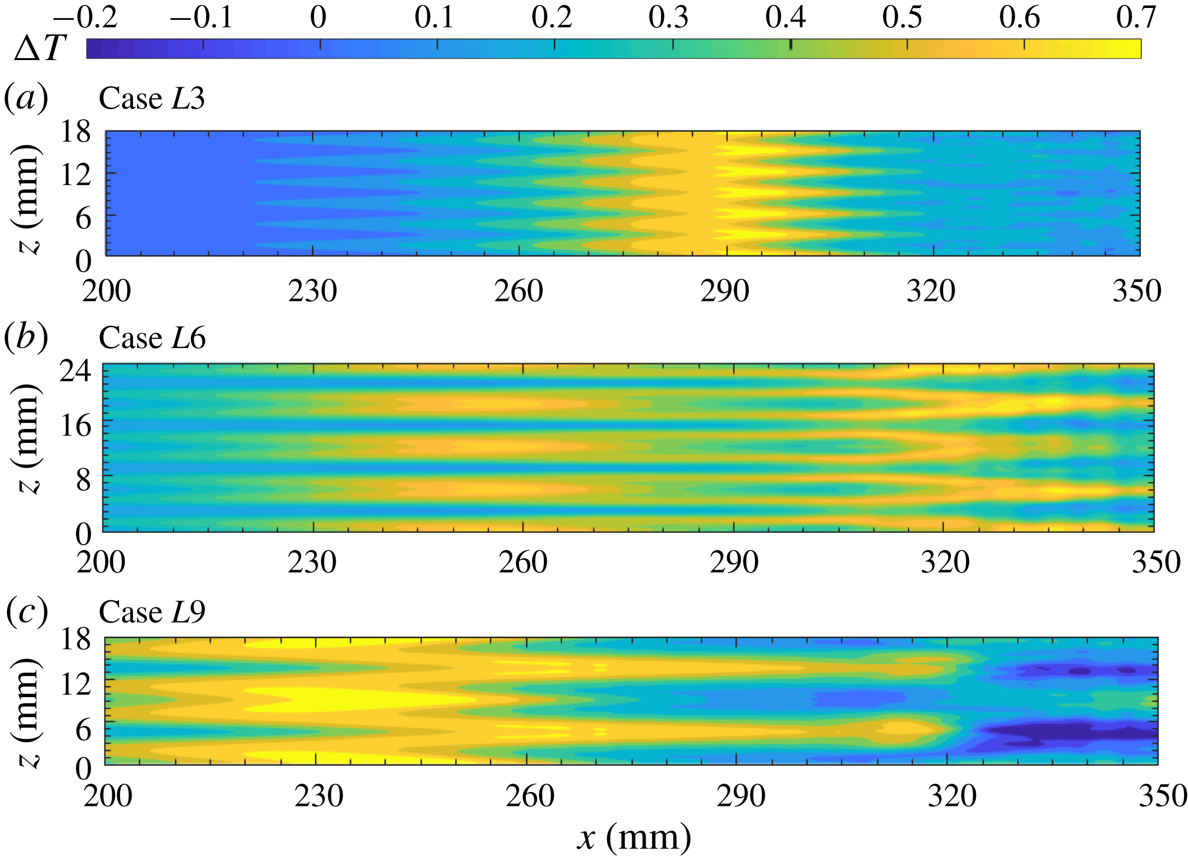
Figure 12. Time-averaged wall temperature variations relative to laminar flow for the three cases.
Increases in temperature or heat flux caused by Görtler vortices have also been repeatedly observed in hypersonic experiments (de Luca et al.
Reference de Luca, Cardone, de la Chevalerie and Fonteneau1993; Chevalerie et al.
Reference Chevalerie, De La Fonteneau, Luca and Cardone1997; Roghelia et al.
Reference Roghelia, Olivier, Egorov and Chuvakhov2017), but the mechanism is still not thoroughly understood. In the incompressible regime, heat transfer induced by Görtler vortices is treated as a linear transport problem, with temperature simply acting as a passive scalar (Liu & Sabry Reference Liu and Sabry1991; Liu Reference Liu2008; Malatesta et al.
Reference Malatesta, Souza, Liu and Kloker2015). As a result, the temperature distribution essentially depends on the velocity distribution. Hypersonic flow, however, is more complex. For example, one can observe in figure 12(a) that the high-temperature streaks initially lie in the high-speed region at
 $x\approx 280~\text{mm}$
and gradually shift to the low-speed region. This cannot be explained by the linear transport equation. One must solve the momentum and energy equations in tandem to predict the temperature distribution. Heat streaks could also emerge in other transition scenarios (Franko & Lele Reference Franko and Lele2013; Sivasubramanian & Fasel Reference Sivasubramanian and Fasel2015). The similarity is that the heat streaks are all generated by (quasi-)streamwise vortices. The difference is that Görtler vortices are unstable and grow by themselves, whereas streamwise vortices in other transition regimes are generated by the nonlinear interaction of first and second Mack-mode waves. It is interesting to note that the temperature increase in the Purdue experiments (Berridge et al.
Reference Berridge, Chou, Ward, Steen, Gilbert, Juliano, Schneider and Gronvall2010; Chou et al.
Reference Chou, Ward, Letterman, Luersen, Borg and Schneider2011), which is believed to be caused by the fundamental breakdown (Sivasubramanian & Fasel Reference Sivasubramanian and Fasel2015), is only approximately 10 K, or 20 % of the static temperature. This indicates that the increase in heat caused by Görtler vortices may be larger than those in other transition regimes.
$x\approx 280~\text{mm}$
and gradually shift to the low-speed region. This cannot be explained by the linear transport equation. One must solve the momentum and energy equations in tandem to predict the temperature distribution. Heat streaks could also emerge in other transition scenarios (Franko & Lele Reference Franko and Lele2013; Sivasubramanian & Fasel Reference Sivasubramanian and Fasel2015). The similarity is that the heat streaks are all generated by (quasi-)streamwise vortices. The difference is that Görtler vortices are unstable and grow by themselves, whereas streamwise vortices in other transition regimes are generated by the nonlinear interaction of first and second Mack-mode waves. It is interesting to note that the temperature increase in the Purdue experiments (Berridge et al.
Reference Berridge, Chou, Ward, Steen, Gilbert, Juliano, Schneider and Gronvall2010; Chou et al.
Reference Chou, Ward, Letterman, Luersen, Borg and Schneider2011), which is believed to be caused by the fundamental breakdown (Sivasubramanian & Fasel Reference Sivasubramanian and Fasel2015), is only approximately 10 K, or 20 % of the static temperature. This indicates that the increase in heat caused by Görtler vortices may be larger than those in other transition regimes.
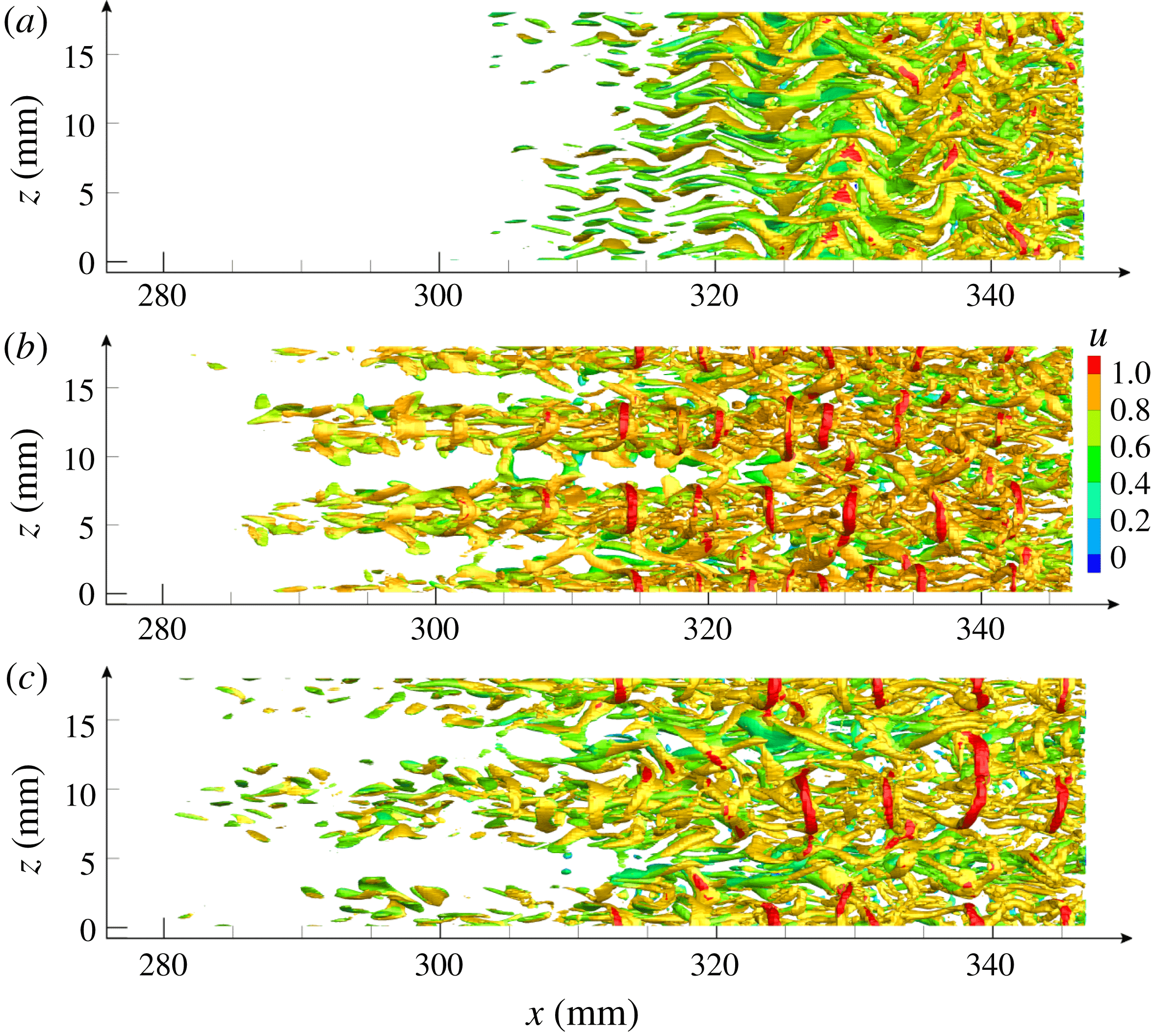
Figure 13. Visualization of flow structures using isosurfaces of
 $Q$
criterion (
$Q$
criterion (
 $Q=0.042$
) for
$Q=0.042$
) for
 $L3$
(a),
$L3$
(a),
 $L6$
(b) and
$L6$
(b) and
 $L9$
(c). The isosurfaces are coloured according to the streamwise velocity magnitude.
$L9$
(c). The isosurfaces are coloured according to the streamwise velocity magnitude.
Finally, the flow structures for all three cases are plotted using the
 $Q$
criterion (Hunt, Wray & Moin Reference Hunt, Wray and Moin1988) in figure 13. Note that we have chosen a relatively large
$Q$
criterion (Hunt, Wray & Moin Reference Hunt, Wray and Moin1988) in figure 13. Note that we have chosen a relatively large
 $Q$
to make the secondary instability structures more prominent. As a result, however, the Görtler vortices become less visible. Figure 13(a) reveals that the flow structures for
$Q$
to make the secondary instability structures more prominent. As a result, however, the Görtler vortices become less visible. Figure 13(a) reveals that the flow structures for
 $L3$
mainly consist of sinuously oscillating streamwise vortices. Such a flow pattern is a typical feature of the sinuous instability, as shown in figure 6. For
$L3$
mainly consist of sinuously oscillating streamwise vortices. Such a flow pattern is a typical feature of the sinuous instability, as shown in figure 6. For
 $L6$
and
$L6$
and
 $L9$
, the flow structures are initially concentrated around the primary streaks, and gradually expand downstream. The near-wall regions are occupied by streamwise vortices, above which hairpin vortices appear periodically. The wavelengths of the hairpin vortices range from 5 to 10 mm in both cases. The hairpin vortices confirm the existence of varicose instabilities in these two cases.
$L9$
, the flow structures are initially concentrated around the primary streaks, and gradually expand downstream. The near-wall regions are occupied by streamwise vortices, above which hairpin vortices appear periodically. The wavelengths of the hairpin vortices range from 5 to 10 mm in both cases. The hairpin vortices confirm the existence of varicose instabilities in these two cases.
4.2 Stability analysis
4.2.1 Fundamental instability
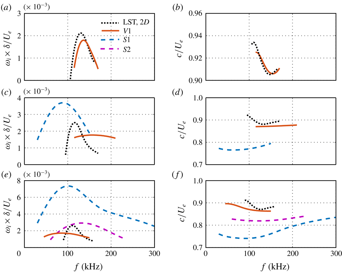
We now consider the stability of the boundary layer in the presence of Görtler vortices. Figure 14 shows the growth rate of the unstable sinuous modes (dashed lines) and varicose modes (solid lines) at various stream locations for
 $L3$
, along with the corresponding phase velocities. Here, the sinuous and varicose modes are defined by the mode shapes, regardless of whether the secondary instability occurs. For simplicity, we denote the sinuous modes as mode
$L3$
, along with the corresponding phase velocities. Here, the sinuous and varicose modes are defined by the mode shapes, regardless of whether the secondary instability occurs. For simplicity, we denote the sinuous modes as mode
 $S1$
, mode
$S1$
, mode
 $S2,\ldots ,$
and varicose modes as mode
$S2,\ldots ,$
and varicose modes as mode
 $V1$
, mode
$V1$
, mode
 $V2,\ldots ,$
according to the order in which they appear. At
$V2,\ldots ,$
according to the order in which they appear. At
 $x=166~\text{mm}$
, only varicose mode
$x=166~\text{mm}$
, only varicose mode
 $V1$
is present, and this is a modified second Mack-mode instability. Compared with the laminar case, this mode is stabilized by Görtler vortices, and its peak frequency first increases and then decreases. Farther downstream, at
$V1$
is present, and this is a modified second Mack-mode instability. Compared with the laminar case, this mode is stabilized by Görtler vortices, and its peak frequency first increases and then decreases. Farther downstream, at
 $x=252~\text{mm}$
, a sinuous mode of secondary instability,
$x=252~\text{mm}$
, a sinuous mode of secondary instability,
 $S1$
, emerges in a low-frequency range with low phase velocities. It quickly becomes significantly unstable with a much wider frequency range at
$S1$
, emerges in a low-frequency range with low phase velocities. It quickly becomes significantly unstable with a much wider frequency range at
 $x=289~\text{mm}$
, where a less unstable sinuous mode,
$x=289~\text{mm}$
, where a less unstable sinuous mode,
 $S2$
, also appears.
$S2$
, also appears.
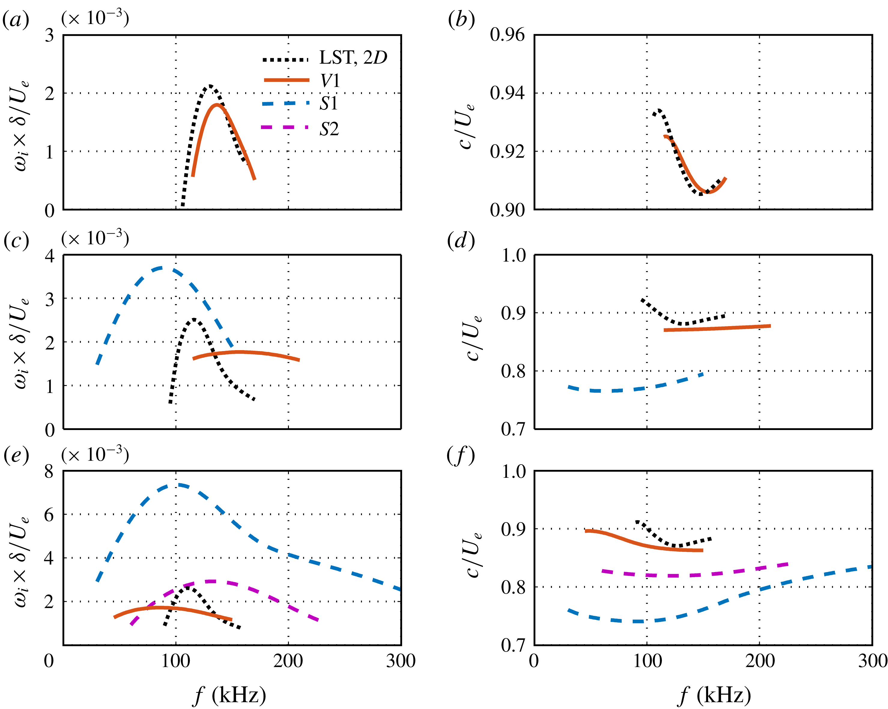
Figure 14. Growth rates of unstable modes (fundamental instability) for
 $L3$
at (a)
$L3$
at (a)
 $x=166~\text{mm}$
, (c)
$x=166~\text{mm}$
, (c)
 $x=252~\text{mm}$
and (e)
$x=252~\text{mm}$
and (e)
 $x=289~\text{mm}$
. The growth rate is normalized by
$x=289~\text{mm}$
. The growth rate is normalized by
 $U_{e}/\unicode[STIX]{x1D6FF}$
, where
$U_{e}/\unicode[STIX]{x1D6FF}$
, where
 $\unicode[STIX]{x1D6FF}=0.0725~\text{mm}$
is the reference length and
$\unicode[STIX]{x1D6FF}=0.0725~\text{mm}$
is the reference length and
 $U_{e}$
is the free stream velocity. The corresponding phase velocities are shown in (b), (d) and (f), respectively. For the local LST results, black dots denote two-dimensional disturbances.
$U_{e}$
is the free stream velocity. The corresponding phase velocities are shown in (b), (d) and (f), respectively. For the local LST results, black dots denote two-dimensional disturbances.
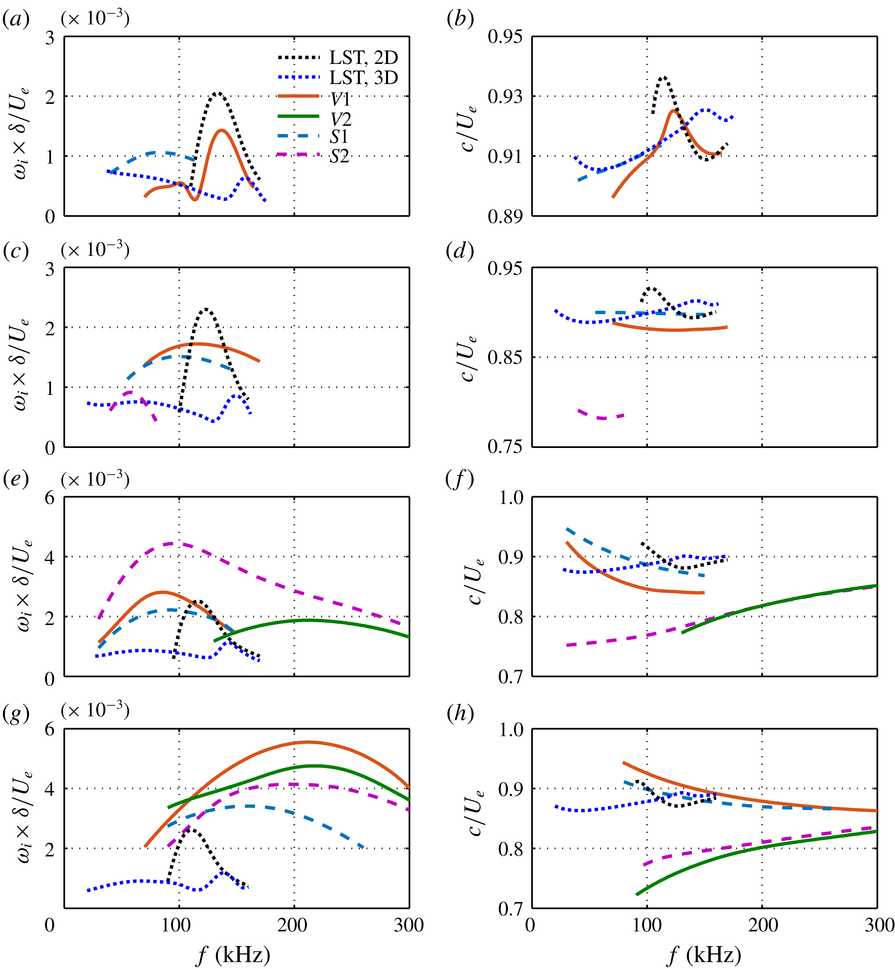
Figure 15. Growth rates of unstable modes (fundamental instability) for
 $L6$
at (a)
$L6$
at (a)
 $x=151~\text{mm}$
, (c)
$x=151~\text{mm}$
, (c)
 $x=212~\text{mm}$
, (e)
$x=212~\text{mm}$
, (e)
 $x=258~\text{mm}$
and (g)
$x=258~\text{mm}$
and (g)
 $x=289~\text{mm}$
. The corresponding phase velocities are shown in (b), (d), (f) and (h), respectively. For the local LST results, black dots denote two-dimensional disturbances and blue dots denote the disturbances with the fundamental spanwise wavelength.
$x=289~\text{mm}$
. The corresponding phase velocities are shown in (b), (d), (f) and (h), respectively. For the local LST results, black dots denote two-dimensional disturbances and blue dots denote the disturbances with the fundamental spanwise wavelength.
Similar stability results were also obtained for
 $L6$
, as depicted in figure 15. The LST results (dotted lines) for the laminar boundary layer are also presented for comparison. The black dotted line represents the second Mack-mode instability, whereas the blue dotted line denotes the Görtler instability (low frequency), the first Mack-mode instability (moderate frequency) and the oblique second Mack-mode instability (high frequency). At
$L6$
, as depicted in figure 15. The LST results (dotted lines) for the laminar boundary layer are also presented for comparison. The black dotted line represents the second Mack-mode instability, whereas the blue dotted line denotes the Görtler instability (low frequency), the first Mack-mode instability (moderate frequency) and the oblique second Mack-mode instability (high frequency). At
 $x=151~\text{mm}$
, where the Görtler vortices are still too small to induce a secondary instability, only (modified) primary instabilities are present. Mode
$x=151~\text{mm}$
, where the Görtler vortices are still too small to induce a secondary instability, only (modified) primary instabilities are present. Mode
 $S1$
is likely to originate from the first Mack-mode instability, having a peak frequency of around 80 kHz and exhibiting an increasing phase velocity with increasing frequency. Mode
$S1$
is likely to originate from the first Mack-mode instability, having a peak frequency of around 80 kHz and exhibiting an increasing phase velocity with increasing frequency. Mode
 $V1$
has two peaks in its growth rate. The lower one probably develops from the first Mack-mode instability, whereas the higher one evolves from the second Mack-mode instability. Comparison with the LST results clearly shows that mode
$V1$
has two peaks in its growth rate. The lower one probably develops from the first Mack-mode instability, whereas the higher one evolves from the second Mack-mode instability. Comparison with the LST results clearly shows that mode
 $V1$
(
$V1$
(
 $S1$
) is stabilized (destabilized) by the Görtler vortices. At
$S1$
) is stabilized (destabilized) by the Görtler vortices. At
 $x\approx 212~\text{mm}$
, mode
$x\approx 212~\text{mm}$
, mode
 $S1$
, which has a higher frequency range, is further destabilized. Mode
$S1$
, which has a higher frequency range, is further destabilized. Mode
 $V1$
moves to a lower frequency range, suggesting that its first Mack-mode component is more destabilized than its second Mack-mode component. Furthermore, a new type of low-frequency sinuous mode,
$V1$
moves to a lower frequency range, suggesting that its first Mack-mode component is more destabilized than its second Mack-mode component. Furthermore, a new type of low-frequency sinuous mode,
 $S2$
, appears. Its phase velocity is much lower than those of the primary instabilities, indicating that it is a secondary instability mode with no origin in the primary instability. Farther downstream, at
$S2$
, appears. Its phase velocity is much lower than those of the primary instabilities, indicating that it is a secondary instability mode with no origin in the primary instability. Farther downstream, at
 $x=258~\text{mm}$
, mode
$x=258~\text{mm}$
, mode
 $V1$
continues to shift to lower frequencies with a slightly enhanced growth rate. In contrast, mode
$V1$
continues to shift to lower frequencies with a slightly enhanced growth rate. In contrast, mode
 $S2$
is significantly enhanced, becoming the most unstable mode, and shifts to a higher frequency range. In addition, a new type of high-frequency varicose mode,
$S2$
is significantly enhanced, becoming the most unstable mode, and shifts to a higher frequency range. In addition, a new type of high-frequency varicose mode,
 $V2$
, emerges. Its phase velocity increases with increasing frequency, like mode
$V2$
, emerges. Its phase velocity increases with increasing frequency, like mode
 $S1$
, whereas the phase velocities of modes
$S1$
, whereas the phase velocities of modes
 $V1$
and
$V1$
and
 $S1$
exhibit the opposite trend. This characteristic may be used to distinguish different types of secondary instability modes. At the last location,
$S1$
exhibit the opposite trend. This characteristic may be used to distinguish different types of secondary instability modes. At the last location,
 $x=289~\text{mm}$
, all modes are remarkably promoted, with mode
$x=289~\text{mm}$
, all modes are remarkably promoted, with mode
 $V2$
growing fastest, followed by mode
$V2$
growing fastest, followed by mode
 $V2$
, mode
$V2$
, mode
 $S2$
and mode
$S2$
and mode
 $S1$
. Moreover, modes
$S1$
. Moreover, modes
 $V1$
and
$V1$
and
 $S1$
, which have higher frequencies and faster growth rates, are now far away from the primary instability range, indicating that these are already secondary-instability modes.
$S1$
, which have higher frequencies and faster growth rates, are now far away from the primary instability range, indicating that these are already secondary-instability modes.
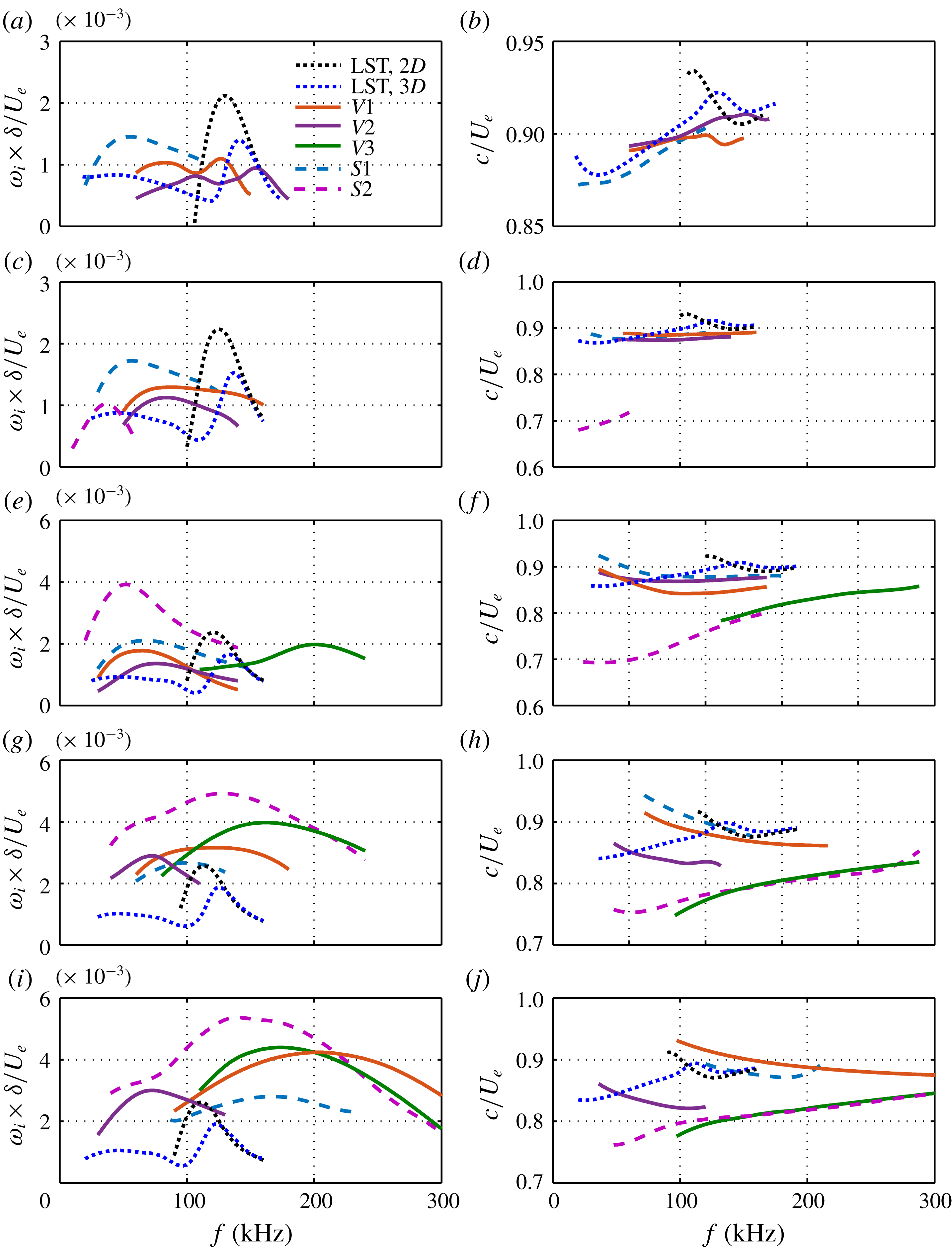
Figure 16. Growth rates of unstable modes (fundamental instability) for
 $L9$
at (a)
$L9$
at (a)
 $x=166~\text{mm}$
, (c)
$x=166~\text{mm}$
, (c)
 $x=197~\text{mm}$
, (e)
$x=197~\text{mm}$
, (e)
 $x=227~\text{mm}$
, (g)
$x=227~\text{mm}$
, (g)
 $x=273~\text{mm}$
and (i)
$x=273~\text{mm}$
and (i)
 $x=289~\text{mm}$
. The corresponding phase velocities are shown in (b), (d), (f), (h) and (j), respectively. For the local LST results, black dots denote two-dimensional disturbances and blue dots denote the disturbances with the fundamental spanwise wavelength.
$x=289~\text{mm}$
. The corresponding phase velocities are shown in (b), (d), (f), (h) and (j), respectively. For the local LST results, black dots denote two-dimensional disturbances and blue dots denote the disturbances with the fundamental spanwise wavelength.
Figure 16 illustrates the downstream evolution of various modes for
 $L9$
. The LST results are also included for comparison. As in case
$L9$
. The LST results are also included for comparison. As in case
 $L6$
, mode
$L6$
, mode
 $S1$
comes from the first Mack-mode instability and is continuously enhanced relative to the laminar case. Its peak frequency remains at around 60 kHz until
$S1$
comes from the first Mack-mode instability and is continuously enhanced relative to the laminar case. Its peak frequency remains at around 60 kHz until
 $x=252~\text{mm}$
, where it starts to rapidly increase. The varicose mode
$x=252~\text{mm}$
, where it starts to rapidly increase. The varicose mode
 $V1$
for
$V1$
for
 $L9$
now splits into two branches, mode
$L9$
now splits into two branches, mode
 $V1$
and mode
$V1$
and mode
 $V2$
, due to stronger secondary streaks than for
$V2$
, due to stronger secondary streaks than for
 $L6$
. Both modes initially consist of first and second Mack-mode components. Later, it will be shown that mode
$L6$
. Both modes initially consist of first and second Mack-mode components. Later, it will be shown that mode
 $V1$
is associated with the primary streaks and mode
$V1$
is associated with the primary streaks and mode
 $V2$
is related to the secondary streaks. Thus, mode
$V2$
is related to the secondary streaks. Thus, mode
 $V1$
behaves like mode
$V1$
behaves like mode
 $V1$
for
$V1$
for
 $L6$
, that is, it first shifts to the low-frequency region with moderate growth rates, and then moves to the high-frequency region with large growth rates. In contrast, mode
$L6$
, that is, it first shifts to the low-frequency region with moderate growth rates, and then moves to the high-frequency region with large growth rates. In contrast, mode
 $V2$
shifts to the first Mack-mode frequency region and remains there. When the streaks attain a sufficiently large amplitude, modes
$V2$
shifts to the first Mack-mode frequency region and remains there. When the streaks attain a sufficiently large amplitude, modes
 $S2$
and
$S2$
and
 $V3$
appear and soon become the most unstable sinuous and varicose modes, respectively.
$V3$
appear and soon become the most unstable sinuous and varicose modes, respectively.
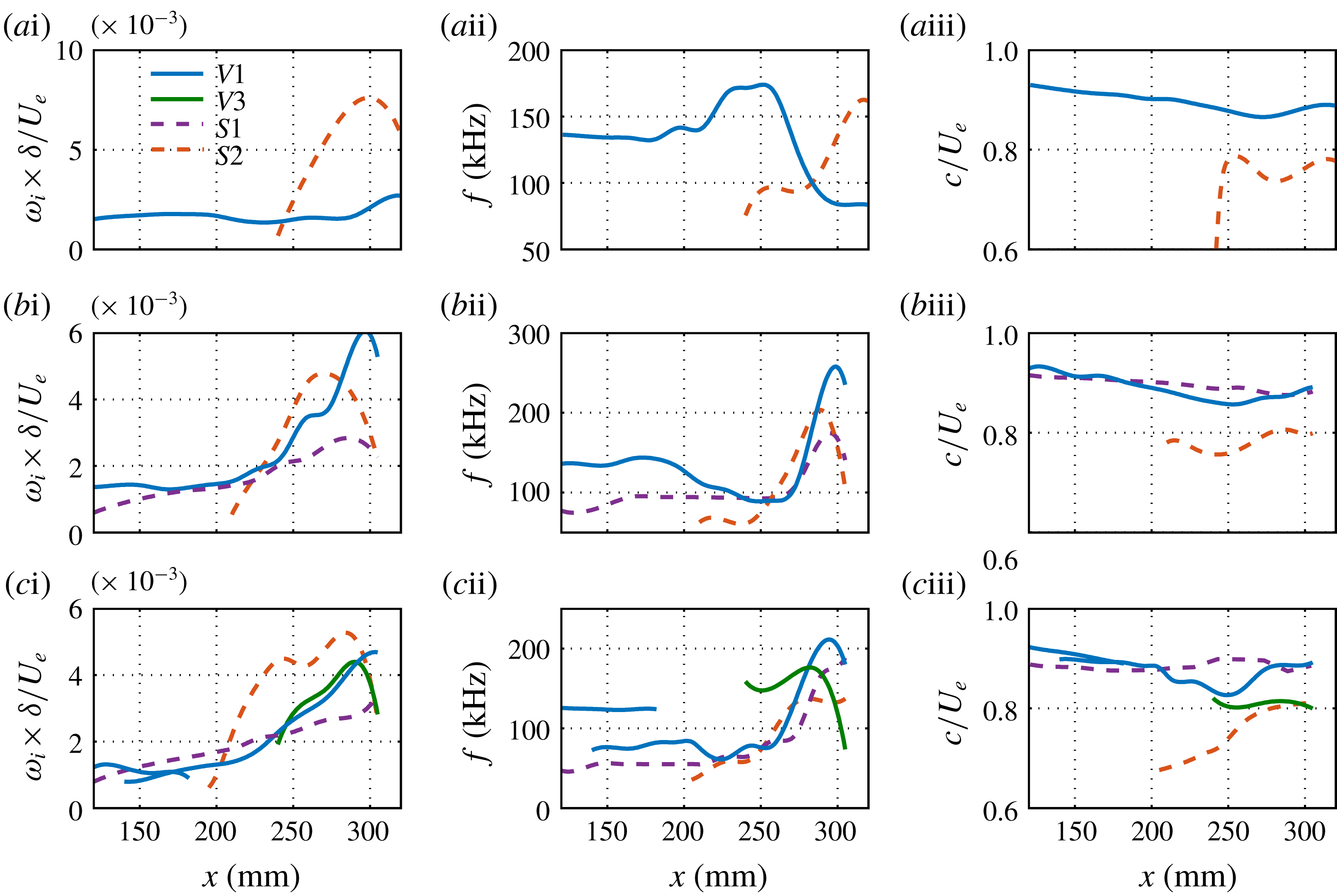
Figure 17. Fundamental instability characteristics for different cases: (a)
 $L3$
, (b)
$L3$
, (b)
 $L6$
and (c)
$L6$
and (c)
 $L9$
. Column (i) presents the maximum spatial growth rate of the sinuous (dashed lines) and varicose (solid lines) modes at various streamwise locations. Columns (ii) and (iii) show the corresponding frequencies and phase velocities.
$L9$
. Column (i) presents the maximum spatial growth rate of the sinuous (dashed lines) and varicose (solid lines) modes at various streamwise locations. Columns (ii) and (iii) show the corresponding frequencies and phase velocities.
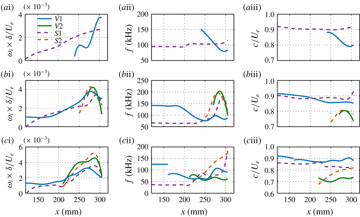
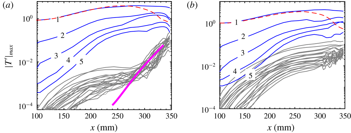
The overall mode evolution in all three cases is summarized in figure 17. Only the modes that produce the locally most unstable varicose or sinuous modes are displayed. By comparing these three cases, we can make some interesting observations. Firstly, the secondary instability occurs earliest for
 $L9$
, then for
$L9$
, then for
 $L6$
and finally for
$L6$
and finally for
 $L3$
. Secondly,
$L3$
. Secondly,
 $L3$
has the maximum growth rate, followed by
$L3$
has the maximum growth rate, followed by
 $L6$
and then
$L6$
and then
 $L9$
. Thirdly, within the secondary-instability regime, the sinuous mode is most unstable for
$L9$
. Thirdly, within the secondary-instability regime, the sinuous mode is most unstable for
 $L3$
and
$L3$
and
 $L9$
, whereas the varicose mode is more dangerous for
$L9$
, whereas the varicose mode is more dangerous for
 $L6$
. As reported by Li & Malik (Reference Li and Malik1995) for the incompressible case, the sinuous mode is the first to become unstable, although the varicose mode catches up farther downstream. Finally, the peak frequencies of almost all the modes increase sharply during the secondary-instability stage.
$L6$
. As reported by Li & Malik (Reference Li and Malik1995) for the incompressible case, the sinuous mode is the first to become unstable, although the varicose mode catches up farther downstream. Finally, the peak frequencies of almost all the modes increase sharply during the secondary-instability stage.
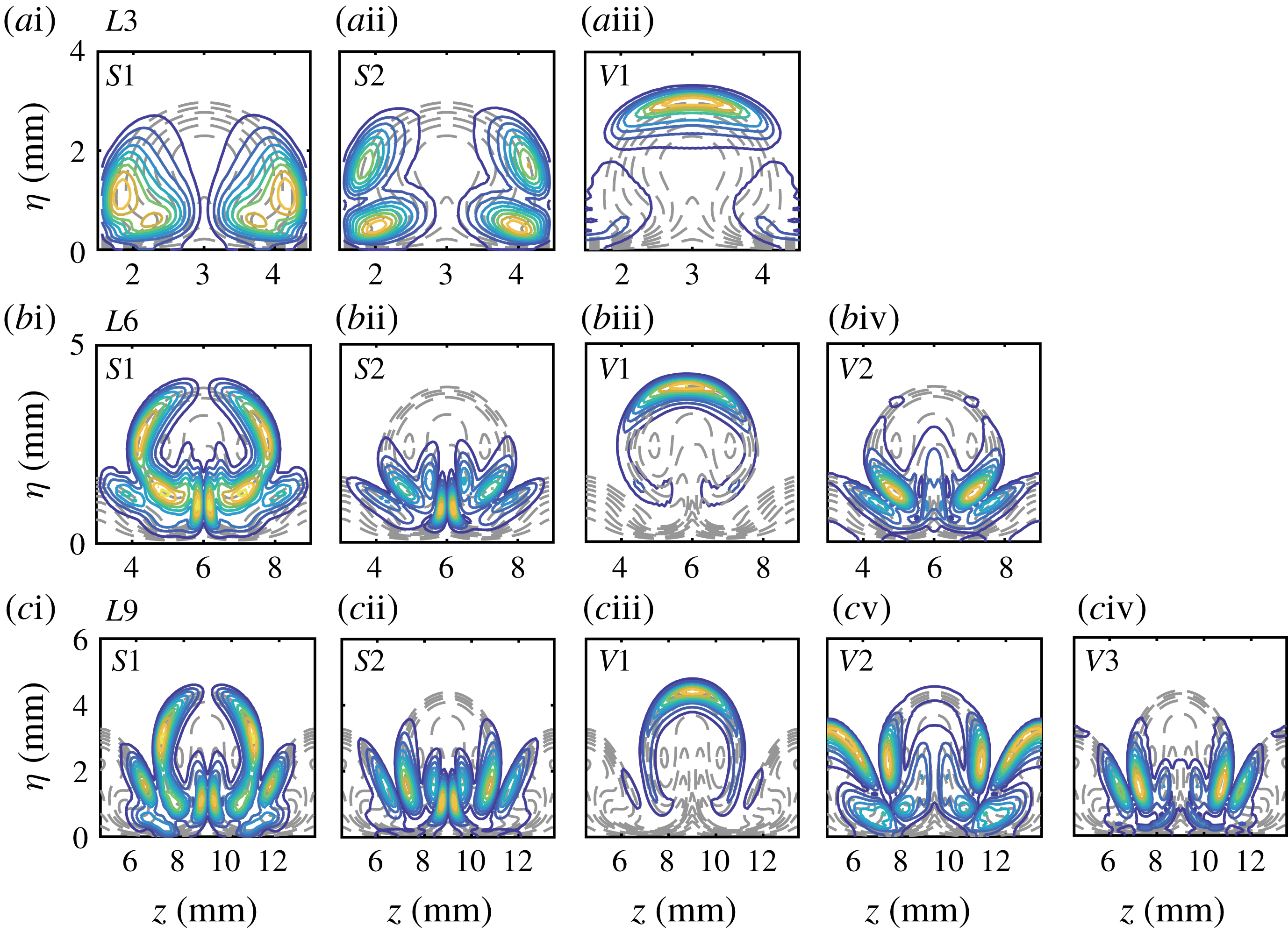
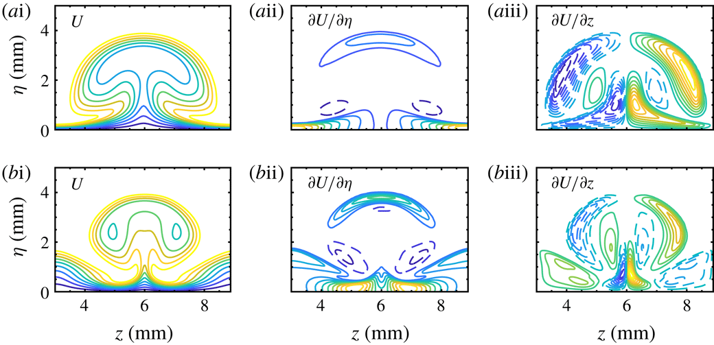
Figure 18. Normalized magnitudes of temperature disturbances for selected unstable secondary modes at
 $x=289~\text{mm}$
in the three cases. Contours of the base flows are also plotted (dashed lines). The contour level increment is 0.1.
$x=289~\text{mm}$
in the three cases. Contours of the base flows are also plotted (dashed lines). The contour level increment is 0.1.
The temperature contours of unstable modes at
 $x=289~\text{mm}$
are shown in figure 18, together with the base flow state (dashed lines) in the background. The frequency of each mode is chosen to be the most amplified one. We note that the main difference between the modes originating from primary instabilities (
$x=289~\text{mm}$
are shown in figure 18, together with the base flow state (dashed lines) in the background. The frequency of each mode is chosen to be the most amplified one. We note that the main difference between the modes originating from primary instabilities (
 $S1$
for
$S1$
for
 $L6$
and
$L6$
and
 $L9$
;
$L9$
;
 $V1$
for all three cases; and
$V1$
for all three cases; and
 $V2$
for
$V2$
for
 $L9$
) and other modes is that the former exhibit a remarkable distribution on the upper part of the mushroom, whereas the latter are only present in the lower part. In particular, mode
$L9$
) and other modes is that the former exhibit a remarkable distribution on the upper part of the mushroom, whereas the latter are only present in the lower part. In particular, mode
 $V3$
for
$V3$
for
 $L9$
is mainly distributed around the top of the secondary-streak structures, indicating that this mode is likely to have been induced by the secondary streaks. The most interesting observation is that mode
$L9$
is mainly distributed around the top of the secondary-streak structures, indicating that this mode is likely to have been induced by the secondary streaks. The most interesting observation is that mode
 $V2$
for
$V2$
for
 $L6$
and mode
$L6$
and mode
 $V3$
for
$V3$
for
 $L9$
are quite different from the typical varicose mode,
$L9$
are quite different from the typical varicose mode,
 $V1$
, but look very similar to mode
$V1$
, but look very similar to mode
 $S2$
in these two cases. This new type of varicose mode has not been reported before. It is likely to play an important role in the breakdown processes of Görtler vortices, as it exhibits remarkable growth rates in the secondary instability stage.
$S2$
in these two cases. This new type of varicose mode has not been reported before. It is likely to play an important role in the breakdown processes of Görtler vortices, as it exhibits remarkable growth rates in the secondary instability stage.
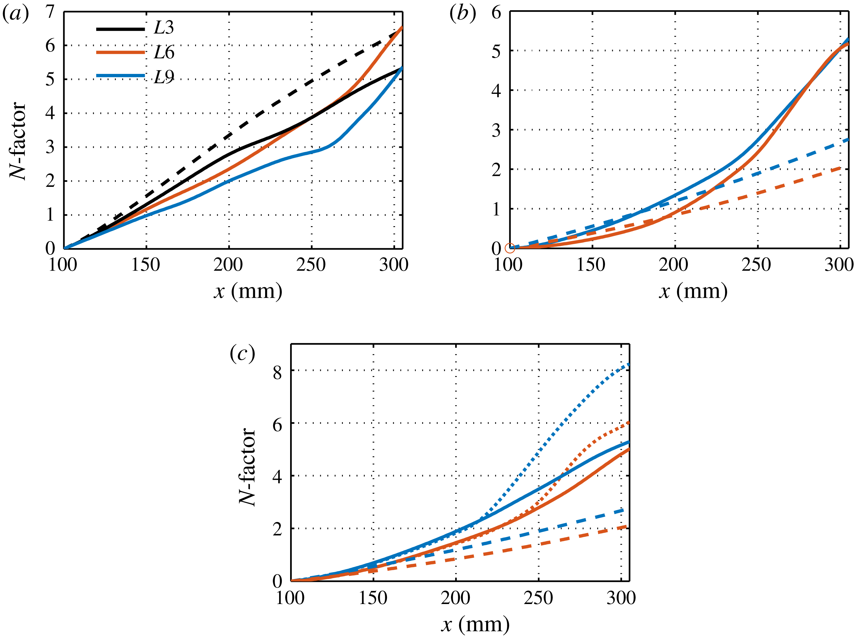
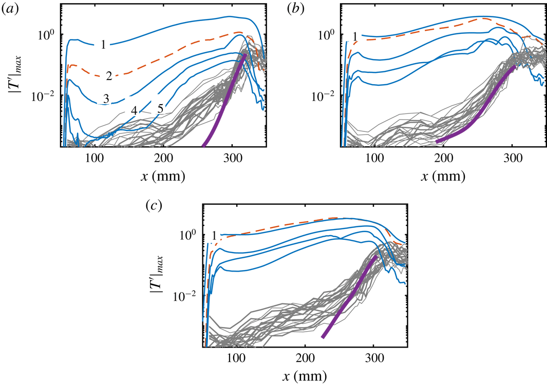
Figure 19.
 $N$
-factors for fundamental primary–secondary modes: (a) second varicose modes with the same frequency of 135 kHz for three cases; (b) first varicose modes with a frequency of 95 kHz for
$N$
-factors for fundamental primary–secondary modes: (a) second varicose modes with the same frequency of 135 kHz for three cases; (b) first varicose modes with a frequency of 95 kHz for
 $L6$
and a frequency of 85 kHz for
$L6$
and a frequency of 85 kHz for
 $L9$
; (c) first sinuous modes with a frequency of 95 kHz for
$L9$
; (c) first sinuous modes with a frequency of 95 kHz for
 $L6$
and a frequency of 58 kHz for
$L6$
and a frequency of 58 kHz for
 $L9$
. The dashed lines denote the corresponding laminar cases. The dotted lines represent the case in which the upstream mode changes to a new type of mode with higher growth rates and lower phase velocities.
$L9$
. The dashed lines denote the corresponding laminar cases. The dotted lines represent the case in which the upstream mode changes to a new type of mode with higher growth rates and lower phase velocities.
The above results indicate that the primary instabilities are remarkably affected by Görtler vortices and may even transform into secondary instabilities. To study them, we examine the spatial evolution of the fixed-frequency disturbances. For simplicity, let the second varicose mode, first varicose mode and first sinuous mode denote the varicose mode from the second Mack mode, the varicose mode from the first Mack mode and the sinuous mode from the first Mack mode, respectively. Figure 19(a) shows the
 $N$
-factors of the second varicose mode (corresponding to mode
$N$
-factors of the second varicose mode (corresponding to mode
 $V1$
in figures 14, 15 and 16) with a frequency of 135 kHz in all three cases, along with the laminar results for comparison. To obtain the
$V1$
in figures 14, 15 and 16) with a frequency of 135 kHz in all three cases, along with the laminar results for comparison. To obtain the
 $N$
-factors, we have converted the temporal growth rate to the spatial one. We can see that the second Mack mode is initially stabilized by the Görtler vortices, and the stabilization effect increases with the blowing–suction wavelength. Farther downstream, the second varicose mode in
$N$
-factors, we have converted the temporal growth rate to the spatial one. We can see that the second Mack mode is initially stabilized by the Görtler vortices, and the stabilization effect increases with the blowing–suction wavelength. Farther downstream, the second varicose mode in
 $L3$
remains less unstable than the second Mack mode in the laminar case, whereas the
$L3$
remains less unstable than the second Mack mode in the laminar case, whereas the
 $N$
-factors for
$N$
-factors for
 $L6$
and
$L6$
and
 $L9$
grow much faster after
$L9$
grow much faster after
 $x=260~\text{mm}$
because of the secondary instability. The overall effect is that the second varicose mode for
$x=260~\text{mm}$
because of the secondary instability. The overall effect is that the second varicose mode for
 $L6$
can reach the same amplitude level as the laminar curve, whereas the second varicose mode in the other two cases is stabilized to some degree.
$L6$
can reach the same amplitude level as the laminar curve, whereas the second varicose mode in the other two cases is stabilized to some degree.
Figure 19(b) depicts the development of the first varicose modes for
 $L6$
and
$L6$
and
 $L9$
with frequencies of 95 and 85 kHz, respectively. It is evident that the first modes, after being slightly stabilized, are strongly destabilized after
$L9$
with frequencies of 95 and 85 kHz, respectively. It is evident that the first modes, after being slightly stabilized, are strongly destabilized after
 $x=200~\text{mm}$
. The resulting
$x=200~\text{mm}$
. The resulting
 $N$
-factors are slightly lower than that of the second varicose mode for
$N$
-factors are slightly lower than that of the second varicose mode for
 $L6$
, but higher than that of the second varicose mode for
$L6$
, but higher than that of the second varicose mode for
 $L9$
. Figure 19(c) illustrates the spatial evolution of the first sinuous modes for
$L9$
. Figure 19(c) illustrates the spatial evolution of the first sinuous modes for
 $L6$
and
$L6$
and
 $L9$
with frequencies of 95 and 58 kHz, respectively. In both cases, the first sinuous modes are moderately promoted by the Görtler vortices if they follow the same type of mode, i.e. mode
$L9$
with frequencies of 95 and 58 kHz, respectively. In both cases, the first sinuous modes are moderately promoted by the Görtler vortices if they follow the same type of mode, i.e. mode
 $S1$
. However, the mode development shown in figures 15 and 16 suggests that the first Mack mode is also likely to become mode
$S1$
. However, the mode development shown in figures 15 and 16 suggests that the first Mack mode is also likely to become mode
 $S2$
(dotted lines) with the same frequency, much higher growth rates and lower phase velocities. Note that there is a discontinuity in the phase velocity between mode
$S2$
(dotted lines) with the same frequency, much higher growth rates and lower phase velocities. Note that there is a discontinuity in the phase velocity between mode
 $S1$
and mode
$S1$
and mode
 $S2$
, and an adjustment region is, thus, required to connect these two modes. A similar adjustment region was observed by Chen, Zhu & Lee (Reference Chen, Zhu and Lee2017) when studying the secondary instability of saturated second Mack-mode waves in a Mach 6 flared-cone boundary layer. In their case, the phase velocities of certain low-frequency modes were largely reduced during the primary–secondary instability transformation process. Because of the adjustment region, the amplitudes of the first sinuous modes would lie between the dotted line and the solid line. Noted also that the evolution of mode
$S2$
, and an adjustment region is, thus, required to connect these two modes. A similar adjustment region was observed by Chen, Zhu & Lee (Reference Chen, Zhu and Lee2017) when studying the secondary instability of saturated second Mack-mode waves in a Mach 6 flared-cone boundary layer. In their case, the phase velocities of certain low-frequency modes were largely reduced during the primary–secondary instability transformation process. Because of the adjustment region, the amplitudes of the first sinuous modes would lie between the dotted line and the solid line. Noted also that the evolution of mode
 $S1$
to mode
$S1$
to mode
 $S2$
may not happen or not be accomplished if the transformation progresses too slowly.
$S2$
may not happen or not be accomplished if the transformation progresses too slowly.

Figure 20. Normalized magnitudes of temperature disturbances of the second varicose modes at various locations for all three cases. The streamwise locations are (i) 151 mm, (ii) 212 mm, (iii) 258 mm and (iv) 289 mm. Contours of the base flows are also plotted (dashed lines). The contour level increment is 0.1.
The spatial evolution of the fixed-frequency disturbances can be further illustrated by the mode shapes. Figure 20 shows the temperature profiles of the second varicose modes at various locations in all three cases. The mode shapes initially exhibit two peaks in the wall-normal direction, one being close to the wall and the other concentrated at the boundary edge, which is a typical feature of the second Mack mode. As the streak amplitude increases, the temperature disturbances gradually become centred around the top of the primary-streak structure.
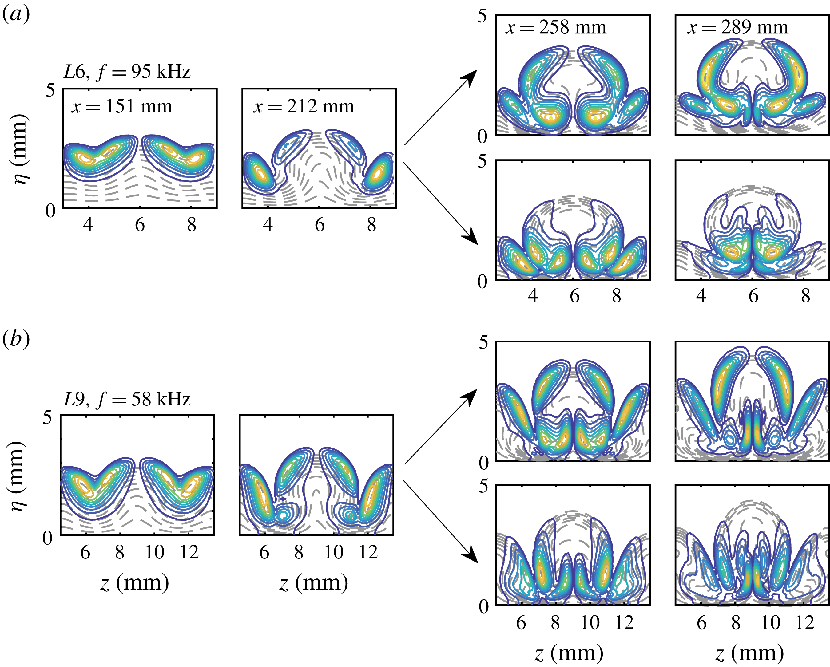
Figure 21. Normalized magnitudes of temperature disturbances of the first sinuous modes at various locations for
 $L6$
and
$L6$
and
 $L9$
. The streamwise locations are (i) 151 mm, (ii) 212 mm, (iii) 258 mm and (iv) 289 mm. Contours of the base flows are also plotted (dashed lines). The contour level increment is 0.1.
$L9$
. The streamwise locations are (i) 151 mm, (ii) 212 mm, (iii) 258 mm and (iv) 289 mm. Contours of the base flows are also plotted (dashed lines). The contour level increment is 0.1.
The temperature distributions of the first sinuous mode at various locations are shown in figure 21. The disturbances are initially concentrated around the boundary layer edge, resembling the first Mack-mode instability. Farther downstream, the first varicose mode follows the evolution of mode
 $S1$
, as denoted by the upright arrow, or changes to the evolution of mode
$S1$
, as denoted by the upright arrow, or changes to the evolution of mode
 $S2$
, as denoted by the downward arrow. Note that both routes are possible because the upstream projections of mode
$S2$
, as denoted by the downward arrow. Note that both routes are possible because the upstream projections of mode
 $S1$
in the downstream region are non-zero for both modes. Because mode
$S1$
in the downstream region are non-zero for both modes. Because mode
 $S2$
grows much faster, its mode shapes gradually come to dominate.
$S2$
grows much faster, its mode shapes gradually come to dominate.
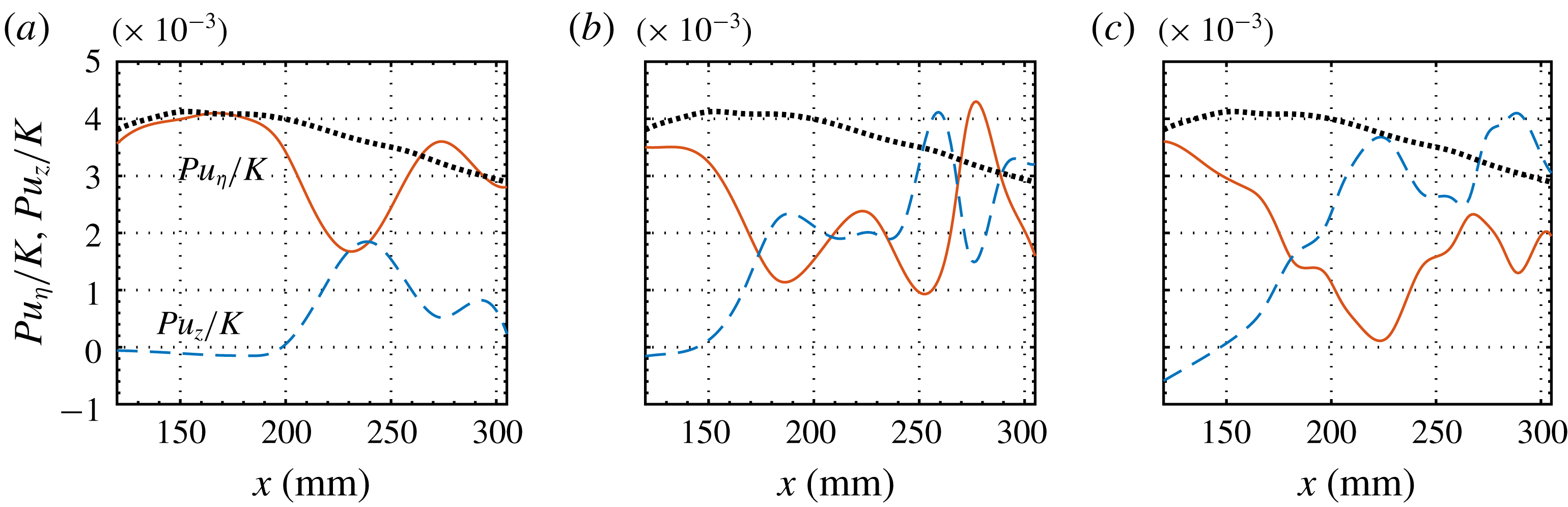
Figure 22. Evolution of the ratio between the production terms associated with the streamwise velocity gradients and the kinetic energy of the perturbation for second varicose modes in figure 19(a): (a)
 $L3$
, (b)
$L3$
, (b)
 $L6$
and (c)
$L6$
and (c)
 $L9$
. The dotted lines represent the laminar case.
$L9$
. The dotted lines represent the laminar case.
To further understand the mechanisms of the effects of Görtler vortices on the primary instability, we calculate the production terms associated with the streamwise velocity gradients for each primary–secondary instability mode. Figure 22 shows the results for the second varicose modes of all three cases, along with the LST results for comparison. The production terms are normalized with the disturbance energy defined by (3.7). As the streaks increase in amplitude, the wall-normal term
 $Pu_{\unicode[STIX]{x1D702}}/K$
rapidly decreases relative to the unperturbed case, which denotes a stabilizing effect, and the spanwise term
$Pu_{\unicode[STIX]{x1D702}}/K$
rapidly decreases relative to the unperturbed case, which denotes a stabilizing effect, and the spanwise term
 $Pu_{z}/K$
notably increases, which denotes a destabilizing effect. The combined effect leads to the stabilization of the second varicose modes. The decrease in
$Pu_{z}/K$
notably increases, which denotes a destabilizing effect. The combined effect leads to the stabilization of the second varicose modes. The decrease in
 $Pu_{\unicode[STIX]{x1D702}}/K$
and increase in
$Pu_{\unicode[STIX]{x1D702}}/K$
and increase in
 $Pu_{z}/K$
can be simply explained by the bending of the base flow, which turns the wall-normal gradient region into the spanwise gradient region. Farther downstream, as the streak amplitudes become larger, the production terms change in each case. For
$Pu_{z}/K$
can be simply explained by the bending of the base flow, which turns the wall-normal gradient region into the spanwise gradient region. Farther downstream, as the streak amplitudes become larger, the production terms change in each case. For
 $L3$
,
$L3$
,
 $Pu_{z}/K$
decreases while
$Pu_{z}/K$
decreases while
 $Pu_{\unicode[STIX]{x1D702}}/K$
increases to become dominant. For
$Pu_{\unicode[STIX]{x1D702}}/K$
increases to become dominant. For
 $L6$
,
$L6$
,
 $Pu_{z}/K$
and
$Pu_{z}/K$
and
 $Pu_{\unicode[STIX]{x1D702}}/K$
have comparable amplitudes and exhibit oscillations. For
$Pu_{\unicode[STIX]{x1D702}}/K$
have comparable amplitudes and exhibit oscillations. For
 $L9$
,
$L9$
,
 $Pu_{z}/K$
is dominant for most of the streamwise stations. This is quite contrary to expectation, as the wall-normal term is usually responsible for the varicose mode (Yu & Liu Reference Yu and Liu1994; Saric Reference Saric1994). The evolution of the production terms for the first varicose modes for
$Pu_{z}/K$
is dominant for most of the streamwise stations. This is quite contrary to expectation, as the wall-normal term is usually responsible for the varicose mode (Yu & Liu Reference Yu and Liu1994; Saric Reference Saric1994). The evolution of the production terms for the first varicose modes for
 $L6$
and
$L6$
and
 $L9$
, shown in figure 23, also demonstrates the dominance of the spanwise production terms. Note that the varicose mode mainly consists of a planar component, which is marginally stable. Therefore, the wall-normal term is much smaller than the LST result based on oblique first Mack-mode waves.
$L9$
, shown in figure 23, also demonstrates the dominance of the spanwise production terms. Note that the varicose mode mainly consists of a planar component, which is marginally stable. Therefore, the wall-normal term is much smaller than the LST result based on oblique first Mack-mode waves.

Figure 23. Evolution of the ratio between the production terms associated with the streamwise velocity gradients and the kinetic energy of the perturbation for first varicose modes in figure 19(b): (a)
 $L6$
and (b)
$L6$
and (b)
 $L9$
. The dotted lines represent the laminar case.
$L9$
. The dotted lines represent the laminar case.
Finally, we examine the energy analysis results for the first sinuous modes for
 $L6$
and
$L6$
and
 $L9$
, as depicted in figure 24. As for the second varicose modes, the wall-normal terms deviate from the laminar cases, showing a stabilizing effect, while the spanwise terms rapidly increase and become dominant. The results for mode
$L9$
, as depicted in figure 24. As for the second varicose modes, the wall-normal terms deviate from the laminar cases, showing a stabilizing effect, while the spanwise terms rapidly increase and become dominant. The results for mode
 $S2$
are also displayed, in which the spanwise terms are remarkably large in both cases.
$S2$
are also displayed, in which the spanwise terms are remarkably large in both cases.
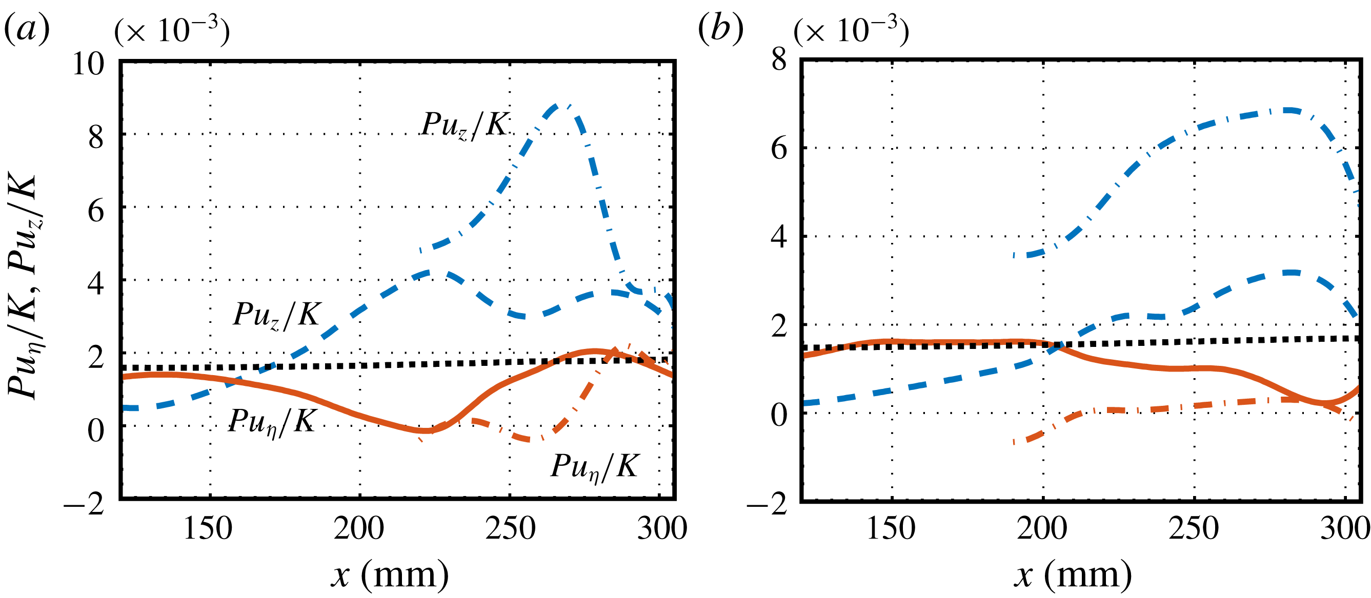
Figure 24. Evolution of the ratio between the production terms associated with the streamwise velocity gradients and the kinetic energy of the perturbation for first sinuous modes in figure 19(c): (a)
 $L6$
and (b)
$L6$
and (b)
 $L9$
. The dotted lines represent the laminar case.
$L9$
. The dotted lines represent the laminar case.
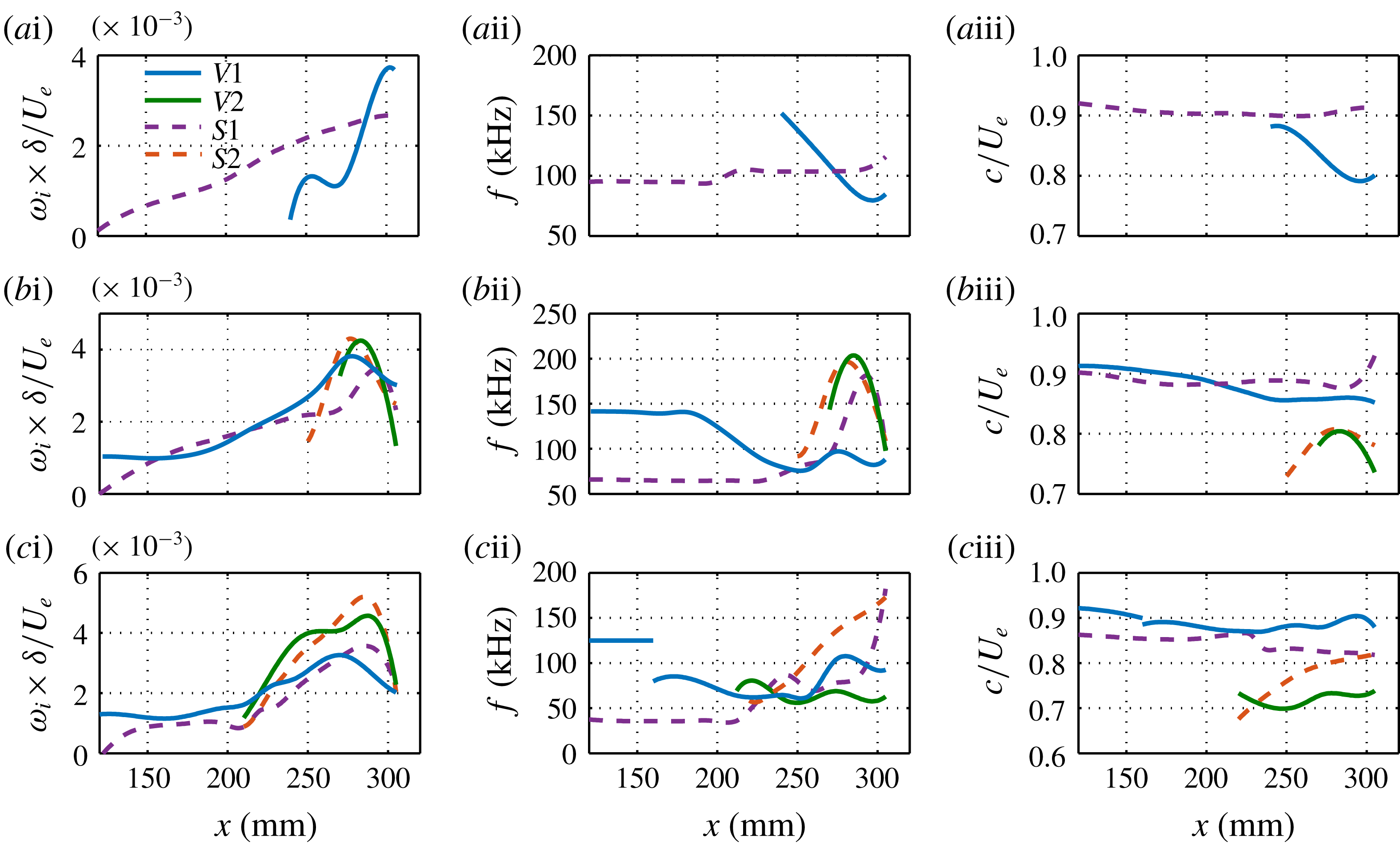
Figure 25. Subharmonic instability characteristics for different cases: (a)
 $L3$
, (b)
$L3$
, (b)
 $L6$
and (c)
$L6$
and (c)
 $L9$
. Column (i) presents the maximum spatial growth rate of the sinuous (dashed lines) and varicose (solid lines) modes at various streamwise locations. Columns (ii) and (iii) show the corresponding frequencies and phase velocities.
$L9$
. Column (i) presents the maximum spatial growth rate of the sinuous (dashed lines) and varicose (solid lines) modes at various streamwise locations. Columns (ii) and (iii) show the corresponding frequencies and phase velocities.
4.2.2 Subharmonic instability
We now consider the subharmonic secondary instability of the Görtler vortices in all three cases. The main stability characteristics are illustrated in figure 25, which depicts the evolution of the most unstable varicose and sinuous modes, and in figure 26, which illustrates the local characteristics at
 $x=289~\text{mm}$
for each mode. The analysis is like that for the fundamental instability, but the results show some differences. In all cases, mode
$x=289~\text{mm}$
for each mode. The analysis is like that for the fundamental instability, but the results show some differences. In all cases, mode
 $S1$
originates from the first Mack-mode instability, with the peak frequency decreasing with increasing wavelength of the blowing and suction. While varicose mode
$S1$
originates from the first Mack-mode instability, with the peak frequency decreasing with increasing wavelength of the blowing and suction. While varicose mode
 $V1$
for
$V1$
for
 $L3$
emerges as a result of the secondary instability far downstream, mode
$L3$
emerges as a result of the secondary instability far downstream, mode
 $V1$
for
$V1$
for
 $L6$
and
$L6$
and
 $L9$
first arises from the second Mack-mode instability, and then amplifies fastest in the first Mack-mode frequency region. Owing to the symmetry, subharmonic second varicose modes arise from oblique second Mack-mode disturbances rather than planar components as in fundamental varicose modes. Therefore, the peak frequency and the growth rates of the second varicose mode depend on the wavelength of the Görtler vortices. In particular, second varicose modes with large wavelengths (as for
$L9$
first arises from the second Mack-mode instability, and then amplifies fastest in the first Mack-mode frequency region. Owing to the symmetry, subharmonic second varicose modes arise from oblique second Mack-mode disturbances rather than planar components as in fundamental varicose modes. Therefore, the peak frequency and the growth rates of the second varicose mode depend on the wavelength of the Görtler vortices. In particular, second varicose modes with large wavelengths (as for
 $L9$
) would be more unstable than those with small wavelengths (as for
$L9$
) would be more unstable than those with small wavelengths (as for
 $L3$
). Farther downstream, secondary instability modes
$L3$
). Farther downstream, secondary instability modes
 $S2$
and
$S2$
and
 $V2$
arise for
$V2$
arise for
 $L6$
and
$L6$
and
 $L9$
, with much lower phase velocities, and soon become dominant. The subharmonic modes for
$L9$
, with much lower phase velocities, and soon become dominant. The subharmonic modes for
 $L6$
and
$L6$
and
 $L9$
can reach growth rates comparable to those of the fundamental ones; thus, both mode types can be observed in the flow visualizations. Although the peak growth rates of subharmonic instabilities for
$L9$
can reach growth rates comparable to those of the fundamental ones; thus, both mode types can be observed in the flow visualizations. Although the peak growth rates of subharmonic instabilities for
 $L3$
are appreciably lower than those of fundamental instabilities, sinuous mode
$L3$
are appreciably lower than those of fundamental instabilities, sinuous mode
 $S1$
can also attain a sufficiently large amplitude to become relevant in the transition, as it amplifies at almost the same peak frequency over most of the simulation region.
$S1$
can also attain a sufficiently large amplitude to become relevant in the transition, as it amplifies at almost the same peak frequency over most of the simulation region.
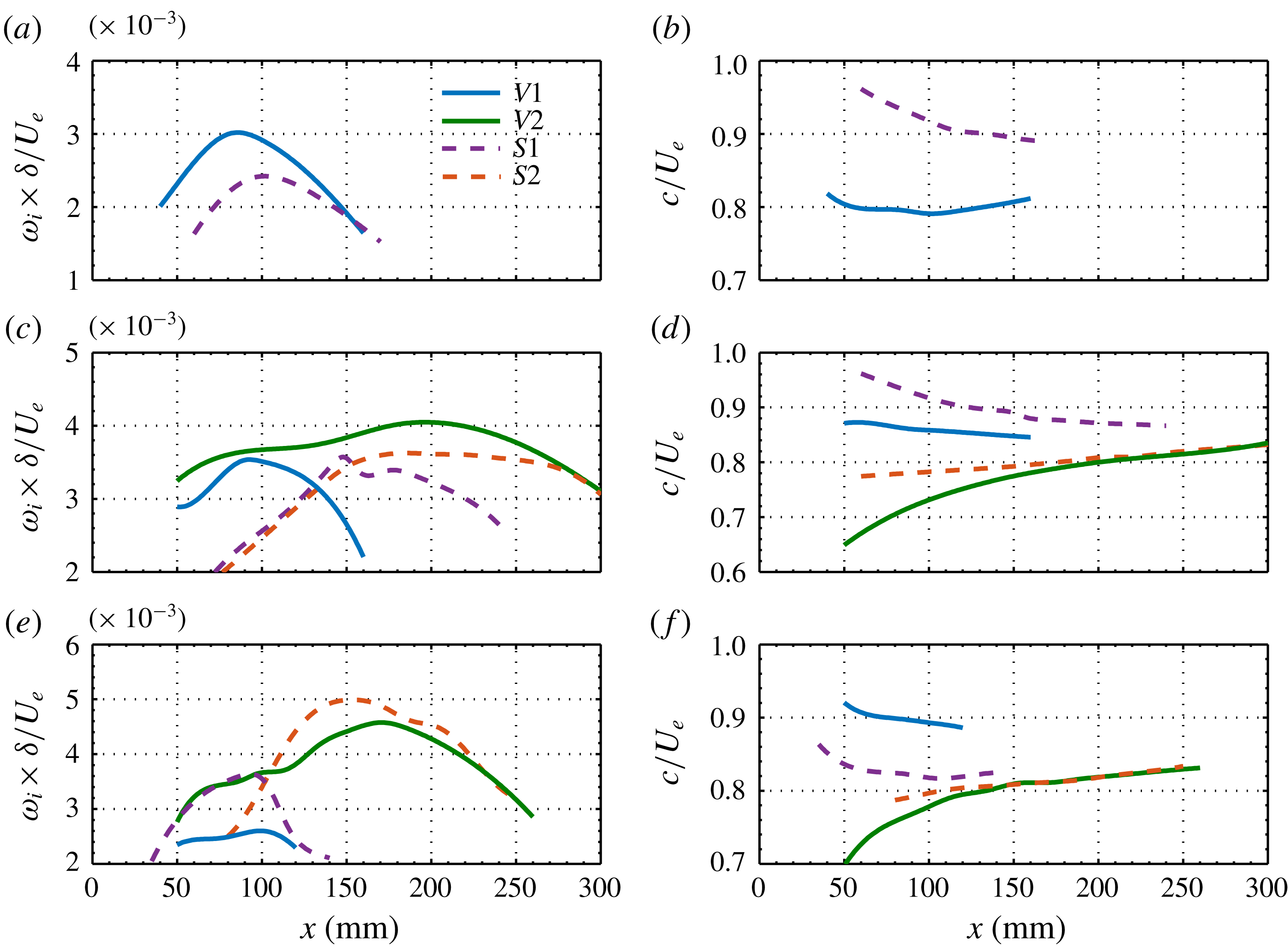
Figure 26. Growth rates of unstable modes (subharmonic instability) at
 $x=289~\text{mm}$
for
$x=289~\text{mm}$
for
 $L3$
(a),
$L3$
(a),
 $L6$
(c) and
$L6$
(c) and
 $L9$
(e). The corresponding phase velocities are plotted in (b), (d) and (f), respectively.
$L9$
(e). The corresponding phase velocities are plotted in (b), (d) and (f), respectively.
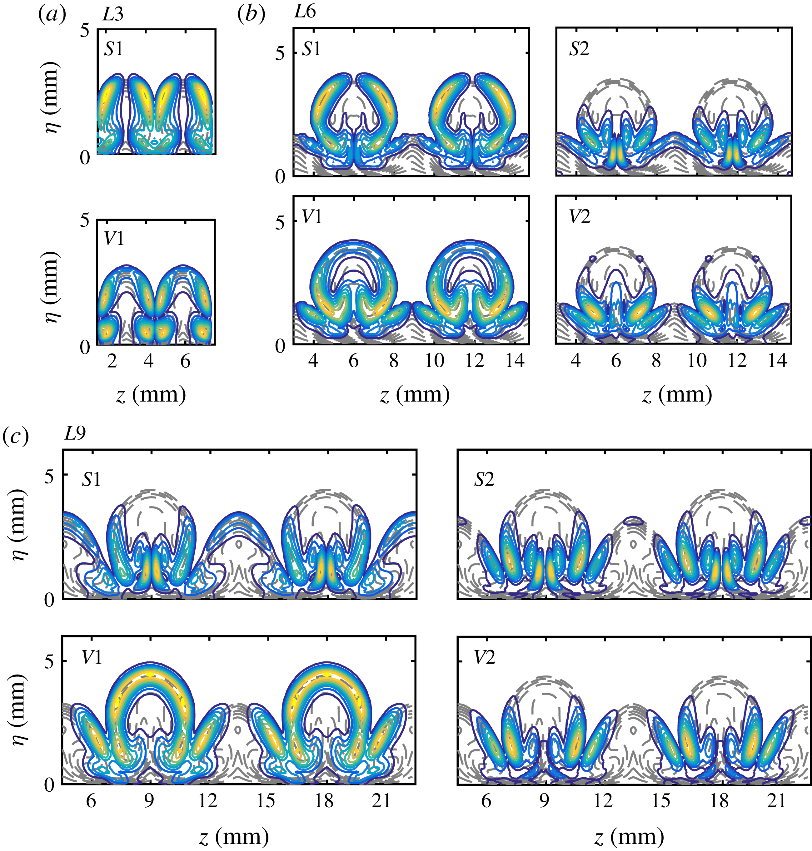
Figure 27. Normalized magnitudes of temperature disturbances of subharmonic modes at
 $x=289~\text{mm}$
for the three cases. Contours of the base flows are also plotted (dashed lines). The contour level increment is 0.1.
$x=289~\text{mm}$
for the three cases. Contours of the base flows are also plotted (dashed lines). The contour level increment is 0.1.
The normalized eigenfunctions (magnitude) of subharmonic modes at
 $x=289~\text{mm}$
are presented in figure 27, together with the base flow state (dashed lines) in the background. The frequency of each mode is selected to correspond with the most amplified instance. Although not shown here, each subharmonic mode undergoes a phase change of 180
$x=289~\text{mm}$
are presented in figure 27, together with the base flow state (dashed lines) in the background. The frequency of each mode is selected to correspond with the most amplified instance. Although not shown here, each subharmonic mode undergoes a phase change of 180
 $^{\circ }$
from one mushroom to the next. These eigenfunctions look like those of the fundamental modes, except for mode
$^{\circ }$
from one mushroom to the next. These eigenfunctions look like those of the fundamental modes, except for mode
 $V1$
in each case, which concentrates in the lower part of the mushroom. A more interesting observation is that the eigenfunctions for
$V1$
in each case, which concentrates in the lower part of the mushroom. A more interesting observation is that the eigenfunctions for
 $L6$
and
$L6$
and
 $L9$
exhibit a mixed-type feature owing to the secondary streaks, that is, the eigenfunctions are symmetric with respect to the primary streaks and antisymmetric with respect to the secondary streaks, and vice versa. This feature is clearly visible in the flow visualizations shown in figures 9(f) and 11(f).
$L9$
exhibit a mixed-type feature owing to the secondary streaks, that is, the eigenfunctions are symmetric with respect to the primary streaks and antisymmetric with respect to the secondary streaks, and vice versa. This feature is clearly visible in the flow visualizations shown in figures 9(f) and 11(f).
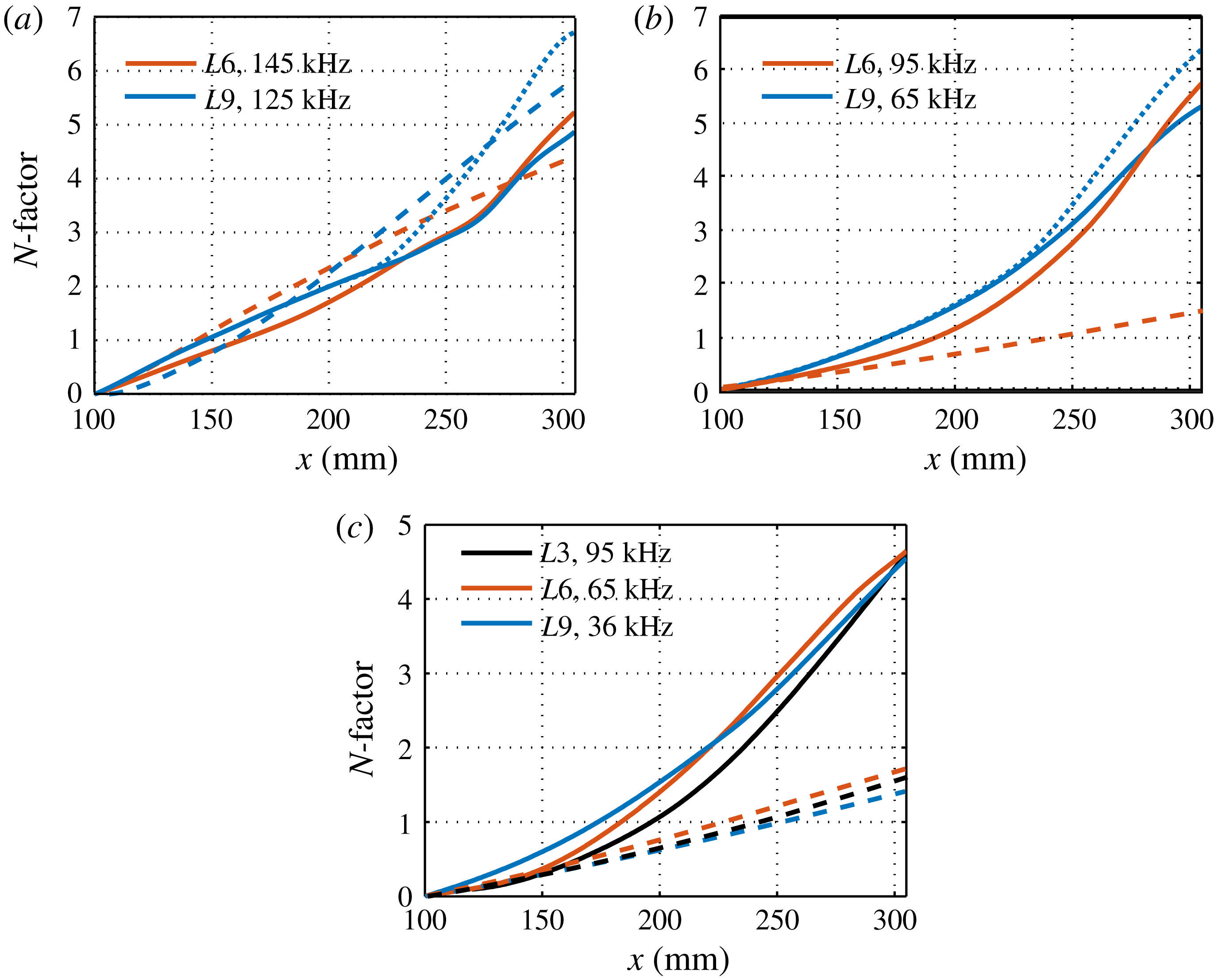
Figure 28.
 $N$
-factors for selected subharmonic primary–secondary modes: (a) second varicose modes with a frequency of 145 kHz for
$N$
-factors for selected subharmonic primary–secondary modes: (a) second varicose modes with a frequency of 145 kHz for
 $L6$
and a frequency of 125 kHz for
$L6$
and a frequency of 125 kHz for
 $L9$
; (b) first varicose modes with a frequency of 95 kHz for
$L9$
; (b) first varicose modes with a frequency of 95 kHz for
 $L6$
and a frequency of 65 kHz for
$L6$
and a frequency of 65 kHz for
 $L9$
; (c) first sinuous modes with a frequency of 95 kHz for
$L9$
; (c) first sinuous modes with a frequency of 95 kHz for
 $L3$
, a frequency of 65 kHz for
$L3$
, a frequency of 65 kHz for
 $L6$
and a frequency of 36 kHz for
$L6$
and a frequency of 36 kHz for
 $L9$
. The dashed lines denote the corresponding laminar cases. The dotted lines represent the case in which the upstream mode changes to a new type of mode with higher growth rates and lower phase velocities.
$L9$
. The dashed lines denote the corresponding laminar cases. The dotted lines represent the case in which the upstream mode changes to a new type of mode with higher growth rates and lower phase velocities.
Next, we examine the possibility of a transformation from a primary to a secondary instability. Like the fundamental counterpart, the second varicose mode is first stabilized and then destabilized when a secondary instability occurs, as shown in figure 28(a). The overall
 $N$
-factors of mode
$N$
-factors of mode
 $V1$
are lower than those of their fundamental counterparts, but mode
$V1$
are lower than those of their fundamental counterparts, but mode
 $V1$
possibly changes to mode
$V1$
possibly changes to mode
 $V2$
to reach a much higher amplitude. The first Mack-mode instability can be converted to both varicose and sinuous secondary instability modes, as depicted in figure 28 (b,c). For the first varicose modes, the selected frequency components of mode
$V2$
to reach a much higher amplitude. The first Mack-mode instability can be converted to both varicose and sinuous secondary instability modes, as depicted in figure 28 (b,c). For the first varicose modes, the selected frequency components of mode
 $V1$
for
$V1$
for
 $L6$
and
$L6$
and
 $L9$
could be continuously enhanced to reach slightly greater
$L9$
could be continuously enhanced to reach slightly greater
 $N$
-factors than their fundamental counterparts. In addition, disturbances from mode
$N$
-factors than their fundamental counterparts. In addition, disturbances from mode
 $V1$
could possibly jump to mode
$V1$
could possibly jump to mode
 $V2$
with higher growth rates and lower phase velocities, resulting in an even larger amplitude. For the first sinuous modes, the selected frequency components of mode
$V2$
with higher growth rates and lower phase velocities, resulting in an even larger amplitude. For the first sinuous modes, the selected frequency components of mode
 $S1$
in all three cases could be continuously amplified, but the
$S1$
in all three cases could be continuously amplified, but the
 $N$
-factors are smaller than those of the first varicose modes. By combining the results of the fundamental and subharmonic instabilities, we can summarize the possible routes for the primary–secondary instability transformation, as shown in figure 29. For
$N$
-factors are smaller than those of the first varicose modes. By combining the results of the fundamental and subharmonic instabilities, we can summarize the possible routes for the primary–secondary instability transformation, as shown in figure 29. For
 $L3$
, only one route likely exists connecting the first Mack mode with the subharmonic sinuous mode. For
$L3$
, only one route likely exists connecting the first Mack mode with the subharmonic sinuous mode. For
 $L6$
and
$L6$
and
 $L9$
, the first Mack mode can be converted to all four kinds of secondary-instability modes, whereas the second Mack mode can only morph into varicose modes.
$L9$
, the first Mack mode can be converted to all four kinds of secondary-instability modes, whereas the second Mack mode can only morph into varicose modes.
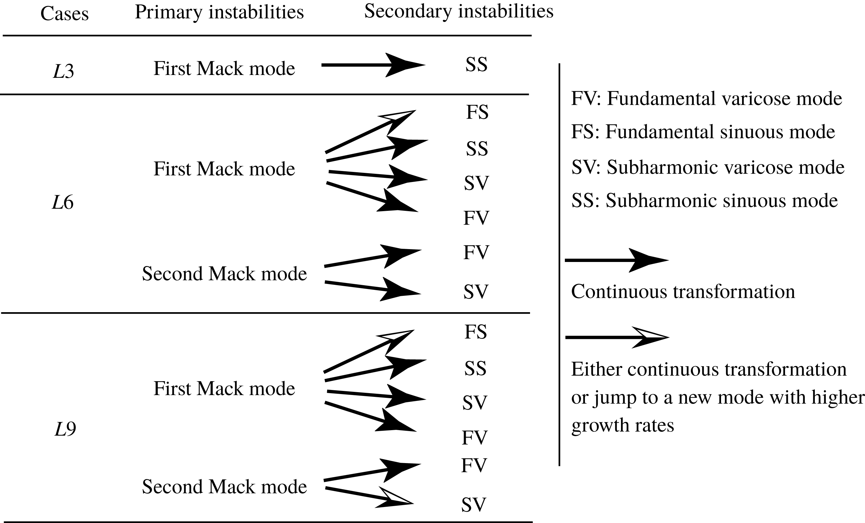
Figure 29. Summary of the primary–secondary instability transformation.
4.3 Statistical results from DNS
In this subsection, we focus on the statistical results from DNS and compare them with those from the stability analysis. Figure 30 shows the mode amplitude evolution for all three cases. For
 $L3$
, the primary mode
$L3$
, the primary mode
 $(0,\unicode[STIX]{x1D6FD})$
first undergoes a transient decay after generation, a common feature in the development of Görtler vortices excited by wall inhomogeneities (Souza et al.
Reference Souza, Mendonca, Medeiros and Kloker2004; Schrader et al.
Reference Schrader, Brandt and Zaki2011), and then starts to grow exponentially at
$(0,\unicode[STIX]{x1D6FD})$
first undergoes a transient decay after generation, a common feature in the development of Görtler vortices excited by wall inhomogeneities (Souza et al.
Reference Souza, Mendonca, Medeiros and Kloker2004; Schrader et al.
Reference Schrader, Brandt and Zaki2011), and then starts to grow exponentially at
 $x\approx 100~\text{mm}$
. Farther downstream, nonlinear processes cause the saturation and decay of this mode. The harmonics evolve similarly. For
$x\approx 100~\text{mm}$
. Farther downstream, nonlinear processes cause the saturation and decay of this mode. The harmonics evolve similarly. For
 $L6$
, the first harmonic quickly grows to an amplitude comparable to that of the primary mode. Then, it soon evolves into a mode with exponential amplification, as its wavelength lies in the linearly unstable region (see figure 4), which is seen as secondary streaks in the visualizations. The initial decay of the primary mode is slower than that for
$L6$
, the first harmonic quickly grows to an amplitude comparable to that of the primary mode. Then, it soon evolves into a mode with exponential amplification, as its wavelength lies in the linearly unstable region (see figure 4), which is seen as secondary streaks in the visualizations. The initial decay of the primary mode is slower than that for
 $L3$
. Therefore, during the receptivity, the Görtler vortices attain larger amplitudes than for
$L3$
. Therefore, during the receptivity, the Görtler vortices attain larger amplitudes than for
 $L3$
, which in turn leads to more developed streak structures and earlier saturation. For
$L3$
, which in turn leads to more developed streak structures and earlier saturation. For
 $L9$
, the first harmonic becomes even more prominent, causing the larger secondary streaks shown in figure 11. Despite this, the amplitude evolution for
$L9$
, the first harmonic becomes even more prominent, causing the larger secondary streaks shown in figure 11. Despite this, the amplitude evolution for
 $L9$
is quite like that for
$L9$
is quite like that for
 $L6$
.
$L6$
.

Figure 30. Amplitude evolution of various modes for three cases: (a)
 $L3$
, (b)
$L3$
, (b)
 $L6$
and (c)
$L6$
and (c)
 $L9$
. The numbers denote the steady modes
$L9$
. The numbers denote the steady modes
 $(0,n\unicode[STIX]{x1D6FD}),n=1,2,3,4,5$
. The first harmonic is depicted by the dashed line. Grey lines represent high-frequency modes
$(0,n\unicode[STIX]{x1D6FD}),n=1,2,3,4,5$
. The first harmonic is depicted by the dashed line. Grey lines represent high-frequency modes
 $(mf_{0},n\unicode[STIX]{x1D6FD}),m=1,2,3,4,5,n=0,1,2,3,f_{0}=50~\text{kHz}$
. Parameter
$(mf_{0},n\unicode[STIX]{x1D6FD}),m=1,2,3,4,5,n=0,1,2,3,f_{0}=50~\text{kHz}$
. Parameter
 $\unicode[STIX]{x1D6FD}$
is the wavenumber of the Görtler mode. Thick lines represent amplitude evolutions based upon the local maximum growth rates predicted by the stability theory.
$\unicode[STIX]{x1D6FD}$
is the wavenumber of the Görtler mode. Thick lines represent amplitude evolutions based upon the local maximum growth rates predicted by the stability theory.
The high-frequency disturbances in figure 30 consist of modes
 $(mf_{0},n\unicode[STIX]{x1D6FD}),m=1,2,3,4,5$
,
$(mf_{0},n\unicode[STIX]{x1D6FD}),m=1,2,3,4,5$
,
 $n=0,1,2,3,f_{0}=50~\text{kHz}$
. These disturbances roughly cover the unstable spectrum predicted by the secondary-instability theory. After generation, these disturbances undergo a long-term complex evolution, with different growth rates for various modes. Farther downstream, the disturbances grow much faster due to the secondary instabilities of the Görtler vortices. The amplitude evolution based on the stability theory is also plotted in the figure, with the slopes indicating the local maximum growth rates. One can see that the disturbances for
$n=0,1,2,3,f_{0}=50~\text{kHz}$
. These disturbances roughly cover the unstable spectrum predicted by the secondary-instability theory. After generation, these disturbances undergo a long-term complex evolution, with different growth rates for various modes. Farther downstream, the disturbances grow much faster due to the secondary instabilities of the Görtler vortices. The amplitude evolution based on the stability theory is also plotted in the figure, with the slopes indicating the local maximum growth rates. One can see that the disturbances for
 $L3$
and
$L3$
and
 $L9$
amplify more slowly than predicted until far downstream. This is because the most unstable modes in the primary- and secondary-instability stages are quite different, and secondary-instability modes require time to become dominant. In contrast, the agreement between DNS and stability theory for
$L9$
amplify more slowly than predicted until far downstream. This is because the most unstable modes in the primary- and secondary-instability stages are quite different, and secondary-instability modes require time to become dominant. In contrast, the agreement between DNS and stability theory for
 $L6$
is generally good over the distances considered, because the dominant
$L6$
is generally good over the distances considered, because the dominant
 $V1$
mode in the primary-instability stage is still (nearly) the most unstable mode in the secondary-instability stage.
$V1$
mode in the primary-instability stage is still (nearly) the most unstable mode in the secondary-instability stage.
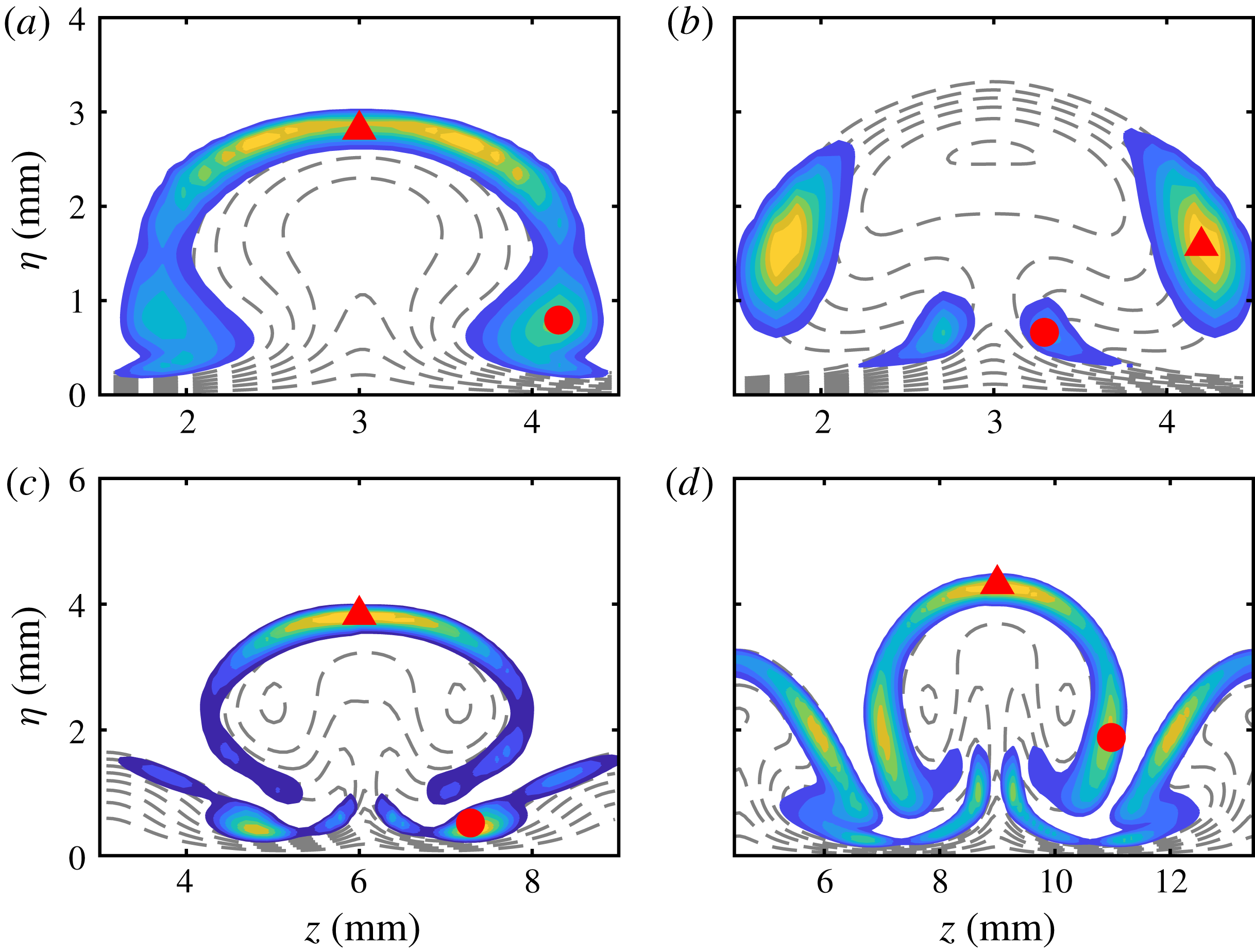
Figure 31. Normalized temperature r.m.s. distribution for three cases: (a)
 $L3$
,
$L3$
,
 $x=289~\text{mm}$
; (b)
$x=289~\text{mm}$
; (b)
 $L3$
,
$L3$
,
 $x=313~\text{mm}$
; (c)
$x=313~\text{mm}$
; (c)
 $L6$
,
$L6$
,
 $x=289~\text{mm}$
; (d)
$x=289~\text{mm}$
; (d)
 $L9$
,
$L9$
,
 $x=289~\text{mm}$
. Symbols represent the time sampling locations in the spectrum analysis.
$x=289~\text{mm}$
. Symbols represent the time sampling locations in the spectrum analysis.
Figure 31 shows the normalized temperature root-mean-square (r.m.s.) distribution from DNS for all three cases at certain locations. For
 $L3$
, the r.m.s. at
$L3$
, the r.m.s. at
 $x=289~\text{mm}$
exhibits a typical varicose-mode distribution with two peaks, one in the top region of the streak and the other in the shoulder region. As discussed above, such an r.m.s. distribution is likely to reflect the primary-instability characteristics, although the sinuous mode of the secondary instability is predicted to be more unstable here. Note that the r.m.s. distribution depends on the upstream evolution process, and does not necessarily match exactly the locally most unstable mode shape. The locally most unstable mode should be more prominent farther downstream, as depicted in figure 31(b). At
$x=289~\text{mm}$
exhibits a typical varicose-mode distribution with two peaks, one in the top region of the streak and the other in the shoulder region. As discussed above, such an r.m.s. distribution is likely to reflect the primary-instability characteristics, although the sinuous mode of the secondary instability is predicted to be more unstable here. Note that the r.m.s. distribution depends on the upstream evolution process, and does not necessarily match exactly the locally most unstable mode shape. The locally most unstable mode should be more prominent farther downstream, as depicted in figure 31(b). At
 $x=313~\text{mm}$
, the r.m.s. distribution is very similar to that of the sinuous mode.
$x=313~\text{mm}$
, the r.m.s. distribution is very similar to that of the sinuous mode.
The r.m.s. distribution for
 $L6$
at
$L6$
at
 $x=289~\text{mm}$
is mainly concentrated around the top region of the primary streak and the shoulder region of the secondary streak. In addition to these two regions, the r.m.s. distribution for
$x=289~\text{mm}$
is mainly concentrated around the top region of the primary streak and the shoulder region of the secondary streak. In addition to these two regions, the r.m.s. distribution for
 $L9$
in the same area also has significant amplitudes in the shoulder and stem regions of the primary streak, as well as the top region of the secondary streak. In both cases, the disturbances in the top region are likely to be caused by the varicose modes, whereas those in the other regions are probably the result of both sinuous and varicose modes.
$L9$
in the same area also has significant amplitudes in the shoulder and stem regions of the primary streak, as well as the top region of the secondary streak. In both cases, the disturbances in the top region are likely to be caused by the varicose modes, whereas those in the other regions are probably the result of both sinuous and varicose modes.
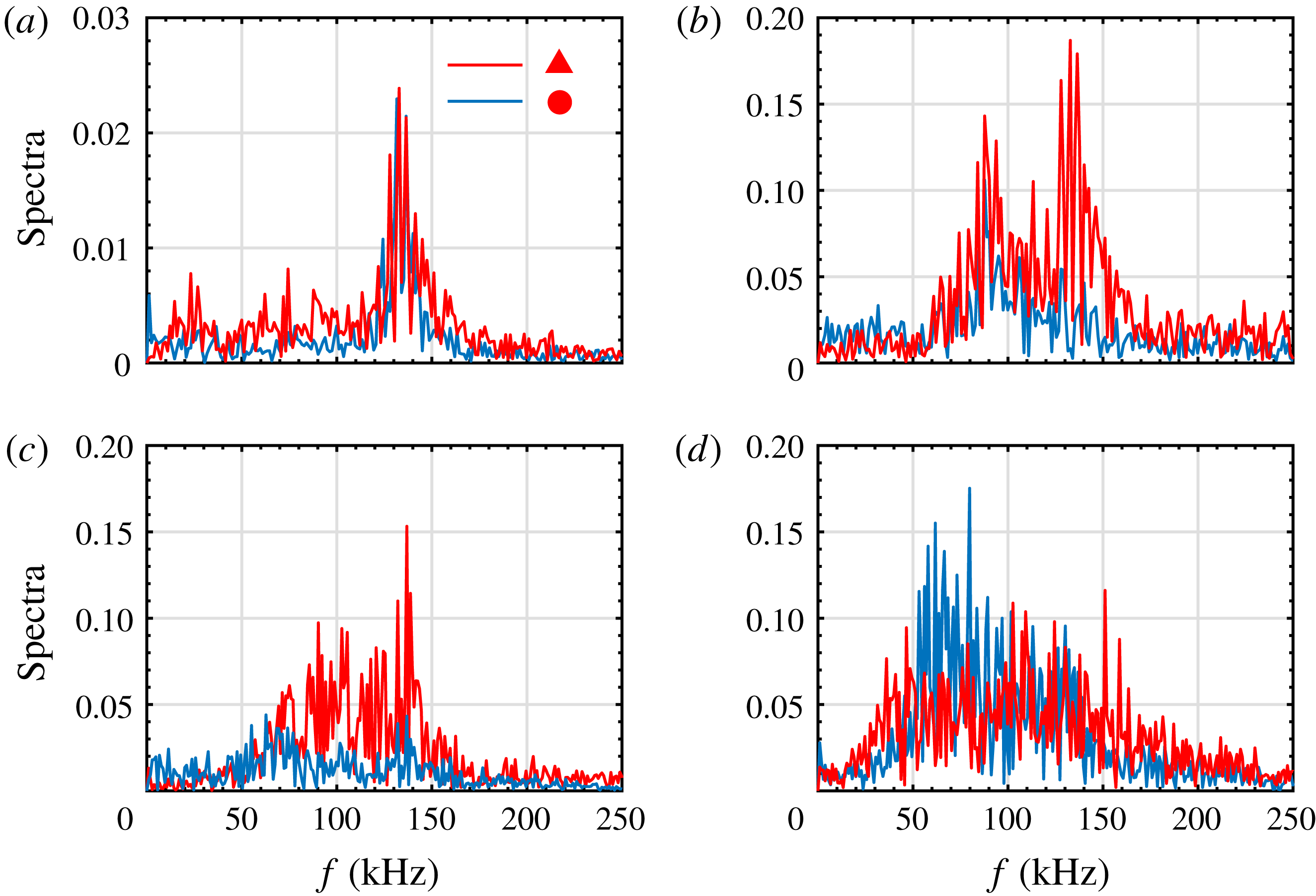
Figure 32. Spectra for the high r.m.s. regions marked in figure 31: (a)
 $L3$
,
$L3$
,
 $x=289~\text{mm}$
; (b)
$x=289~\text{mm}$
; (b)
 $L3$
,
$L3$
,
 $x=313~\text{mm}$
; (c) L6,
$x=313~\text{mm}$
; (c) L6,
 $x=289~\text{mm}$
; (d)
$x=289~\text{mm}$
; (d)
 $L9$
,
$L9$
,
 $x=289~\text{mm}$
. For (b), the red and blue lines represent the spectra in the shoulder and stem regions, respectively. For the other three plots, the red and blue lines represent the spectra in the top and shoulder regions, respectively.
$x=289~\text{mm}$
. For (b), the red and blue lines represent the spectra in the shoulder and stem regions, respectively. For the other three plots, the red and blue lines represent the spectra in the top and shoulder regions, respectively.
Studying the spectra may help to clarify further the components of the disturbances. Figure 32 shows the spectra at the sampling points marked in figure 31. Note that the spectra in the shoulder and stem of the primary streak and in the shoulder of the secondary streak for
 $L6$
and
$L6$
and
 $L9$
are very similar; hence, we need to sample at only one of these regions for each case. For
$L9$
are very similar; hence, we need to sample at only one of these regions for each case. For
 $L3$
at
$L3$
at
 $x=289~\text{mm}$
, the spectra at both sampling points exhibit a significant peak at
$x=289~\text{mm}$
, the spectra at both sampling points exhibit a significant peak at
 $f\approx 135~\text{kHz}$
, which corresponds to the second varicose instability. Farther downstream, at
$f\approx 135~\text{kHz}$
, which corresponds to the second varicose instability. Farther downstream, at
 $x=313~\text{mm}$
, a new peak centred at
$x=313~\text{mm}$
, a new peak centred at
 $f\approx 90~\text{kHz}$
appears in the spectra at both sampling points, which is likely to be related to the secondary instabilities. The frequency peak at
$f\approx 90~\text{kHz}$
appears in the spectra at both sampling points, which is likely to be related to the secondary instabilities. The frequency peak at
 $f\approx 135~\text{kHz}$
, although invisible in the stem region, is still present in the shoulder region. For
$f\approx 135~\text{kHz}$
, although invisible in the stem region, is still present in the shoulder region. For
 $L6$
, the top disturbances have a wide spectrum, ranging from 90 to 140 kHz, with the largest component at around 135 kHz. The frequency peak indicates the significance of the second varicose mode, whereas the lower frequency components are likely to be associated with other secondary-instability modes. In particular, the amplitude of the second varicose mode is much larger than that for
$L6$
, the top disturbances have a wide spectrum, ranging from 90 to 140 kHz, with the largest component at around 135 kHz. The frequency peak indicates the significance of the second varicose mode, whereas the lower frequency components are likely to be associated with other secondary-instability modes. In particular, the amplitude of the second varicose mode is much larger than that for
 $L3$
at the same location, which is consistent with the amplitude evolution predicted by the stability theory (figure 19). The spectrum in the shoulder region has two peaks with much smaller amplitudes, one at around 70 kHz and the other at approximately 135 kHz. For
$L3$
at the same location, which is consistent with the amplitude evolution predicted by the stability theory (figure 19). The spectrum in the shoulder region has two peaks with much smaller amplitudes, one at around 70 kHz and the other at approximately 135 kHz. For
 $L9$
, the disturbances at the top also have a wide spectrum, ranging from 50 to 140 kHz, with the largest component at around 60 kHz. This frequency peak coincides with the peak frequency of (fundamental and subharmonic) first sinuous modes before the onset of the secondary instability, highlighting the role played by the primary instability. The spectrum in the shoulder region is more uniformly distributed from 40 to 160 kHz.
$L9$
, the disturbances at the top also have a wide spectrum, ranging from 50 to 140 kHz, with the largest component at around 60 kHz. This frequency peak coincides with the peak frequency of (fundamental and subharmonic) first sinuous modes before the onset of the secondary instability, highlighting the role played by the primary instability. The spectrum in the shoulder region is more uniformly distributed from 40 to 160 kHz.
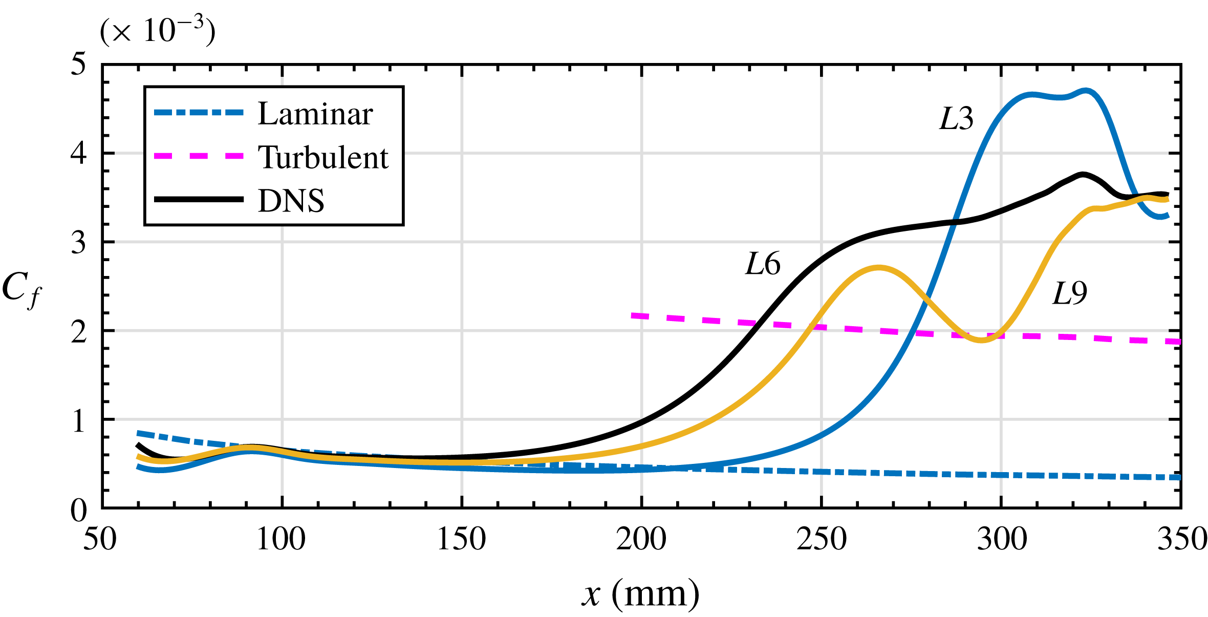
Figure 33. Skin friction coefficient averaged in span and time for the three cases.
Figure 33 displays the time-averaged skin friction for the three cases. The skin friction coefficient was calculated as
 $$\begin{eqnarray}C_{f}=\frac{2\unicode[STIX]{x1D707}(\unicode[STIX]{x2202}\bar{u}/\unicode[STIX]{x2202}\unicode[STIX]{x1D702})|_{\unicode[STIX]{x1D702}=0}}{Re}.\end{eqnarray}$$
The values obtained from the simulations are compared with a turbulent boundary layer correlation from White (Reference White2006) (p. 558). The skin friction curves initially show large defects due to the blowing–suction perturbation, then recover and follow the laminar curve. Farther downstream, the skin friction for
 $L6$
is the first to depart from the laminar curve, followed by those for
$L6$
is the first to depart from the laminar curve, followed by those for
 $L9$
and
$L9$
and
 $L3$
, before rapidly increasing well above the turbulent curve and remaining at a high level. The skin friction for
$L3$
, before rapidly increasing well above the turbulent curve and remaining at a high level. The skin friction for
 $L9$
rapidly decreases after
$L9$
rapidly decreases after
 $x=260~\text{mm}$
and increases again after
$x=260~\text{mm}$
and increases again after
 $x=300~\text{mm}$
, which seem to be caused by the decay of the Görtler vortices and the growth of secondary disturbances, respectively. These two factors are also likely to control the skin-shear evolution in the other two cases, resulting in a slight change for
$x=300~\text{mm}$
, which seem to be caused by the decay of the Görtler vortices and the growth of secondary disturbances, respectively. These two factors are also likely to control the skin-shear evolution in the other two cases, resulting in a slight change for
 $L6$
when the two are almost balanced, and causing a rapid decay for
$L6$
when the two are almost balanced, and causing a rapid decay for
 $L3$
when the former is dominant. Nevertheless, the skin friction in all three cases overshoots the turbulent value, which is a prominent feature of Görtler vortices and streamwise vortices (Kravchenko, Choi & Moin Reference Kravchenko, Choi and Moin1993; Schultz & Volino Reference Schultz and Volino2003; Girgis & Liu Reference Girgis and Liu2006; Tandiono, Winoto & Shah Reference Winoto and Shah2009; Franko & Lele Reference Franko and Lele2013). Moreover, the skin friction does not return to the turbulent value by the end of the simulation, suggesting that the flow fields in these three cases do not have fully developed turbulence.
$L3$
when the former is dominant. Nevertheless, the skin friction in all three cases overshoots the turbulent value, which is a prominent feature of Görtler vortices and streamwise vortices (Kravchenko, Choi & Moin Reference Kravchenko, Choi and Moin1993; Schultz & Volino Reference Schultz and Volino2003; Girgis & Liu Reference Girgis and Liu2006; Tandiono, Winoto & Shah Reference Winoto and Shah2009; Franko & Lele Reference Franko and Lele2013). Moreover, the skin friction does not return to the turbulent value by the end of the simulation, suggesting that the flow fields in these three cases do not have fully developed turbulence.
4.4 Instability of filtered Görtler vortices
To clarify the effects of the first harmonic/secondary streaks on the secondary instability of the primary streaks for
 $L6$
and
$L6$
and
 $L9$
, we eliminate the harmonics at
$L9$
, we eliminate the harmonics at
 $x=80~\text{mm}$
, immediately after the blowing–suction region, and simulate the evolution of the filtered Görtler vortices. The corresponding simulations are denoted as
$x=80~\text{mm}$
, immediately after the blowing–suction region, and simulate the evolution of the filtered Görtler vortices. The corresponding simulations are denoted as
 $FL6$
and
$FL6$
and
 $FL9$
, respectively.
$FL9$
, respectively.
Figure 34 presents the temperature contours at various distances from the wall for
 $FL6$
. Note that the secondary streaks disappear. One can see that both sinuous and varicose instabilities occur, causing the streaks to meander near the wall and the formation of knotty structures above. Compared with the unfiltered case displayed in figure 8, the flow structures are much simpler and the secondary instabilities emerge farther downstream. The end views of the flow structures are shown in figure 35. Again, the secondary streaks are absent, and the mushroom structures start to break down farther downstream than in the unfiltered case. Figure 36 displays the evolution of the mode amplitude for two cases. Several observations can be made. First, the harmonics now have low amplitudes and are essentially driven by the primary mode. Second, the amplitudes of the primary modes in both the filtered and unfiltered cases match well until
$FL6$
. Note that the secondary streaks disappear. One can see that both sinuous and varicose instabilities occur, causing the streaks to meander near the wall and the formation of knotty structures above. Compared with the unfiltered case displayed in figure 8, the flow structures are much simpler and the secondary instabilities emerge farther downstream. The end views of the flow structures are shown in figure 35. Again, the secondary streaks are absent, and the mushroom structures start to break down farther downstream than in the unfiltered case. Figure 36 displays the evolution of the mode amplitude for two cases. Several observations can be made. First, the harmonics now have low amplitudes and are essentially driven by the primary mode. Second, the amplitudes of the primary modes in both the filtered and unfiltered cases match well until
 $x\approx 250~\text{mm}$
. Farther downstream, the primary modes in the unfiltered cases are largely attenuated, whereas the primary modes in the filtered cases remain saturated. This discrepancy is caused by the intensity of the secondary instability, that is, the secondary instability becomes much weaker in the absence of the strong first harmonic. Therefore, we can conclude that the harmonics in unfiltered cases do not directly interact with the primary mode. Instead, they strongly enhance the secondary instability of the Görtler vortices.
$x\approx 250~\text{mm}$
. Farther downstream, the primary modes in the unfiltered cases are largely attenuated, whereas the primary modes in the filtered cases remain saturated. This discrepancy is caused by the intensity of the secondary instability, that is, the secondary instability becomes much weaker in the absence of the strong first harmonic. Therefore, we can conclude that the harmonics in unfiltered cases do not directly interact with the primary mode. Instead, they strongly enhance the secondary instability of the Görtler vortices.
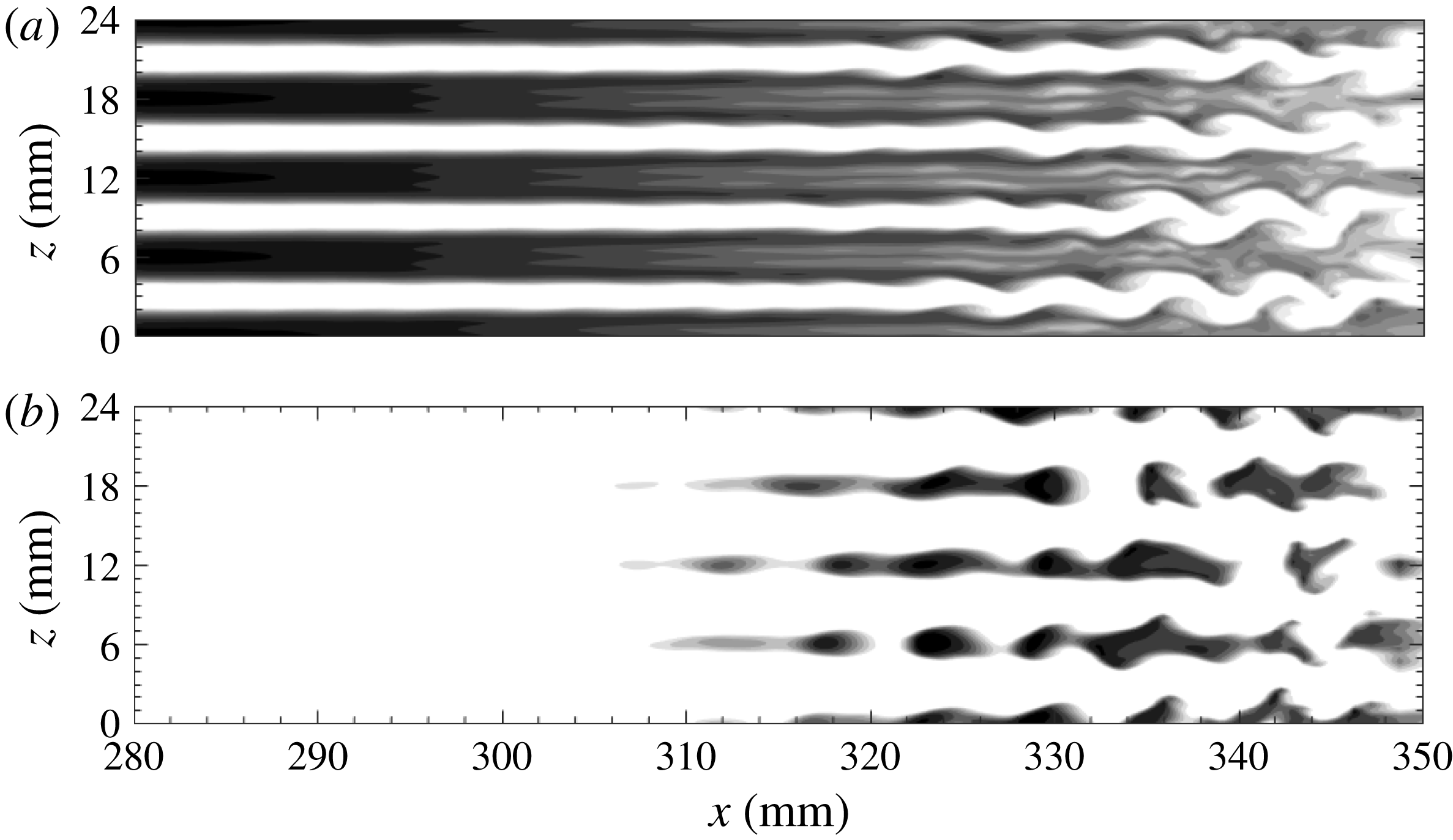
Figure 34. Temperature contours at various distances from the wall for
 $FL6$
: (a)
$FL6$
: (a)
 $\unicode[STIX]{x1D702}=2.43~\text{mm}$
; (b)
$\unicode[STIX]{x1D702}=2.43~\text{mm}$
; (b)
 $\unicode[STIX]{x1D702}=4.07~\text{mm}$
.
$\unicode[STIX]{x1D702}=4.07~\text{mm}$
.
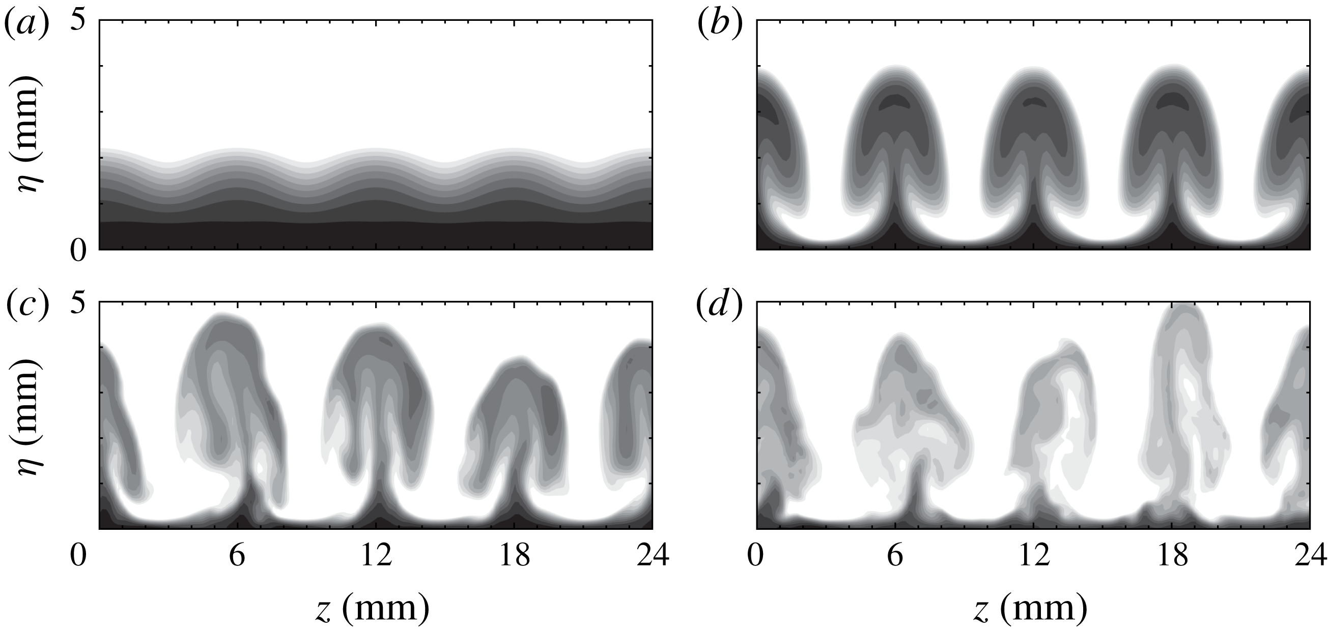
Figure 35. Temperature contours at various streamwise locations for
 $FL6$
: (a)
$FL6$
: (a)
 $x=105~\text{mm}$
; (b)
$x=105~\text{mm}$
; (b)
 $x=304~\text{mm}$
; (c)
$x=304~\text{mm}$
; (c)
 $x=335~\text{mm}$
; (d)
$x=335~\text{mm}$
; (d)
 $x=347~\text{mm}$
.
$x=347~\text{mm}$
.
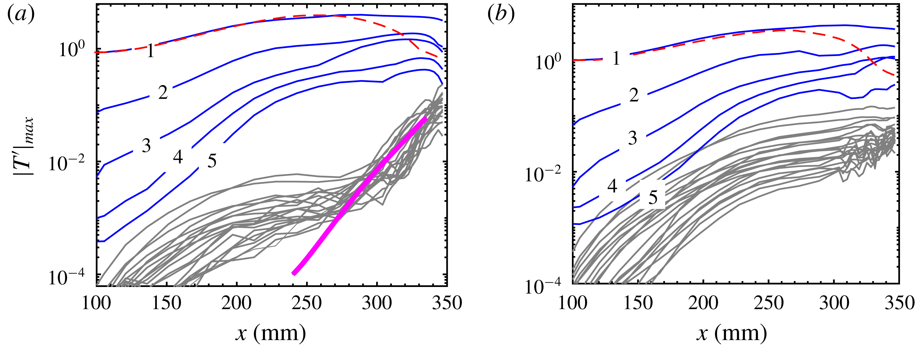
Figure 36. Amplitude evolution of various modes for two cases: (a)
 $FL6$
and (b)
$FL6$
and (b)
 $FL9$
. The numbers denote the steady modes
$FL9$
. The numbers denote the steady modes
 $(0,n\unicode[STIX]{x1D6FD}),n=1,2,3,4,5$
. The primary mode in the unfiltered cases is represented by the dashed line. Grey lines represent high-frequency modes
$(0,n\unicode[STIX]{x1D6FD}),n=1,2,3,4,5$
. The primary mode in the unfiltered cases is represented by the dashed line. Grey lines represent high-frequency modes
 $(mf_{0},n\unicode[STIX]{x1D6FD}),m=1,2,3,4,5,n=0,1,2,3,f_{0}=50~\text{kHz}$
. Parameter
$(mf_{0},n\unicode[STIX]{x1D6FD}),m=1,2,3,4,5,n=0,1,2,3,f_{0}=50~\text{kHz}$
. Parameter
 $\unicode[STIX]{x1D6FD}$
is the wavenumber of the Görtler mode. Thick lines represent the amplitude evolution based upon the local maximum growth rates predicted by the stability theory.
$\unicode[STIX]{x1D6FD}$
is the wavenumber of the Görtler mode. Thick lines represent the amplitude evolution based upon the local maximum growth rates predicted by the stability theory.
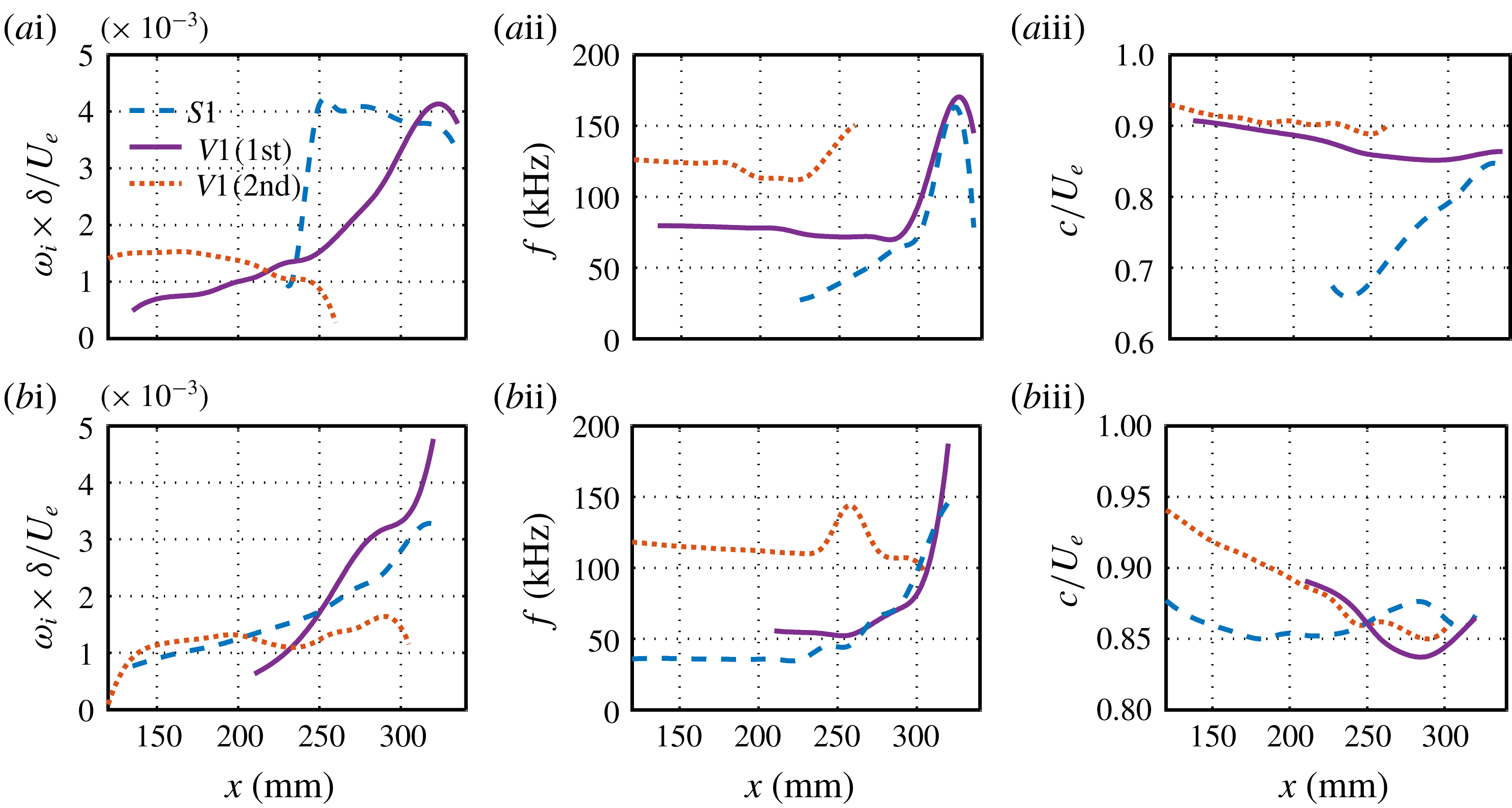
Figure 37. Fundamental instability characteristics (a) and subharmonic instability characteristics (b) for
 $FL6$
. Column (i) presents the downstream evolution of the maximum spatial growth rate of the sinuous mode (dashed lines), the first Mack-mode components of the varicose mode (solid lines) and the second Mack-mode components of the varicose mode. Columns (ii) and (iii) show the corresponding frequencies and phase velocities.
$FL6$
. Column (i) presents the downstream evolution of the maximum spatial growth rate of the sinuous mode (dashed lines), the first Mack-mode components of the varicose mode (solid lines) and the second Mack-mode components of the varicose mode. Columns (ii) and (iii) show the corresponding frequencies and phase velocities.

Figure 38. Mean streamwise velocity contours (i), wall-normal shear (
 $\unicode[STIX]{x2202}U/\unicode[STIX]{x2202}\unicode[STIX]{x1D702}$
) contours (ii) and spanwise shear (
$\unicode[STIX]{x2202}U/\unicode[STIX]{x2202}\unicode[STIX]{x1D702}$
) contours (ii) and spanwise shear (
 $\unicode[STIX]{x2202}U/\unicode[STIX]{x2202}z$
) contours (iii) on the
$\unicode[STIX]{x2202}U/\unicode[STIX]{x2202}z$
) contours (iii) on the
 $z$
–
$z$
–
 $\unicode[STIX]{x1D702}$
plane at
$\unicode[STIX]{x1D702}$
plane at
 $x=289~\text{mm}$
for
$x=289~\text{mm}$
for
 $FL6$
(a) and
$FL6$
(a) and
 $L6$
(b). The contours have been normalized by the maximum values. Dashed lines denote negative values. The contour level increment is 0.1.
$L6$
(b). The contours have been normalized by the maximum values. Dashed lines denote negative values. The contour level increment is 0.1.
To support the above conclusion, we calculated the stability along the streamwise direction. The results are summarized in figure 37. The stability calculations for
 $FL9$
do not indicate an unstable secondary-instability mode, which is consistent with the amplitude evolutions from DNS, and are, therefore, not shown here. For the fundamental instability, the varicose mode
$FL9$
do not indicate an unstable secondary-instability mode, which is consistent with the amplitude evolutions from DNS, and are, therefore, not shown here. For the fundamental instability, the varicose mode
 $V1$
is firstly dominated by the second-varicose components, and then overtaken by the first-varicose components for
$V1$
is firstly dominated by the second-varicose components, and then overtaken by the first-varicose components for
 $x>230~\text{mm}$
. The sinuous mode appears as a secondary-instability mode when the streak amplitude becomes large enough, and soon becomes more unstable than the varicose mode until very far downstream. The peak growth rate of the sinuous mode is comparable with that in the unfiltered case, although the varicose mode is much less unstable. For the subharmonic instability, both varicose and sinuous modes seem to arise from the primary instabilities, and appear to be less unstable than those in the unfiltered case. The oblique second-varicose components are initially dominant, whereas the first-varicose components turn out to be more unstable for
$x>230~\text{mm}$
. The sinuous mode appears as a secondary-instability mode when the streak amplitude becomes large enough, and soon becomes more unstable than the varicose mode until very far downstream. The peak growth rate of the sinuous mode is comparable with that in the unfiltered case, although the varicose mode is much less unstable. For the subharmonic instability, both varicose and sinuous modes seem to arise from the primary instabilities, and appear to be less unstable than those in the unfiltered case. The oblique second-varicose components are initially dominant, whereas the first-varicose components turn out to be more unstable for
 $x>210~\text{mm}$
. The sinuous mode emerges from the first Mack-mode instability. The theoretical evolution of disturbance amplitudes based on the locally most unstable mode is displayed in figure 36(a). The broadband disturbances roughly follow the evolution of the most unstable modes for
$x>210~\text{mm}$
. The sinuous mode emerges from the first Mack-mode instability. The theoretical evolution of disturbance amplitudes based on the locally most unstable mode is displayed in figure 36(a). The broadband disturbances roughly follow the evolution of the most unstable modes for
 $x>290~\text{mm}$
. In conclusion, the filtered case is more stable than the unfiltered case; this supports the idea that destabilization is caused by the secondary streaks. The destabilization mechanism can be understood by examining the base flows in the unfiltered and filtered cases. As shown in figure 38, the primary streak for
$x>290~\text{mm}$
. In conclusion, the filtered case is more stable than the unfiltered case; this supports the idea that destabilization is caused by the secondary streaks. The destabilization mechanism can be understood by examining the base flows in the unfiltered and filtered cases. As shown in figure 38, the primary streak for
 $L6$
appears to be finer (i.e. narrowed by the secondary streaks), and therefore has more intense streamwise velocity gradients. These, in turn, act as the source of the disturbance energy.
$L6$
appears to be finer (i.e. narrowed by the secondary streaks), and therefore has more intense streamwise velocity gradients. These, in turn, act as the source of the disturbance energy.
Figure 39. Skin friction coefficient averaged in span and time for the filtered cases (solid lines). The results for the unfiltered cases (dotted lines) are included for comparison.
Finally, we compare the skin friction evolution with the unfiltered cases in figure 39. One can see that the locations at which the skin friction curves start to depart from the laminar curve are further downstream. Like the unfiltered cases, the skin friction overshoots the turbulent curve by a comparable degree, even though the secondary instability is much weaker. The remarkable decay in the skin friction for
 $L9$
is not observed for
$L9$
is not observed for
 $FL9$
, because the Görtler vortices for
$FL9$
, because the Görtler vortices for
 $FL9$
remain saturated rather than rapidly decaying. The increase in the skin friction for
$FL9$
remain saturated rather than rapidly decaying. The increase in the skin friction for
 $FL6$
near the end of the simulation is likely to be caused by the secondary instability.
$FL6$
near the end of the simulation is likely to be caused by the secondary instability.
5 Summary and discussion
The transition of stationary Görtler vortices in a hypersonic curved-wall boundary layer has been studied in detail using DNS and stability analysis. Görtler vortices were triggered by steady blowing and suction on the wall, for three spanwise wavelengths, i.e. 3 mm (
 $L3$
), 6 mm (
$L3$
), 6 mm (
 $L6$
) and 9 mm (
$L6$
) and 9 mm (
 $L9$
), covering the main part of the Görtler instability according to LST. Görtler vortices induce low-speed streaks in the flow field. In addition to primary streaks with the same wavelength as the blowing and suction, secondary streaks with half the fundamental wavelength also emerge for
$L9$
), covering the main part of the Görtler instability according to LST. Görtler vortices induce low-speed streaks in the flow field. In addition to primary streaks with the same wavelength as the blowing and suction, secondary streaks with half the fundamental wavelength also emerge for
 $L6$
and
$L6$
and
 $L9$
. Downstream, the streaks develop into mushroom structures and subsequently break down through the various mechanisms of secondary instabilities. For
$L9$
. Downstream, the streaks develop into mushroom structures and subsequently break down through the various mechanisms of secondary instabilities. For
 $L3$
, the sinuous-mode instability dominates the breakdown process, whereas for
$L3$
, the sinuous-mode instability dominates the breakdown process, whereas for
 $L6$
the varicose-mode instability is most dangerous. For
$L6$
the varicose-mode instability is most dangerous. For
 $L9$
, sinuous- and varicose-mode instabilities appear to be of equal importance, with the former controlling the near-wall region and the latter appearing on the top of the mushroom structures. Both fundamental and subharmonic instabilities were calculated systematically. The results indicate that the peak growth rates of the subharmonic instability are comparable with those of the fundamental instability for
$L9$
, sinuous- and varicose-mode instabilities appear to be of equal importance, with the former controlling the near-wall region and the latter appearing on the top of the mushroom structures. Both fundamental and subharmonic instabilities were calculated systematically. The results indicate that the peak growth rates of the subharmonic instability are comparable with those of the fundamental instability for
 $L9$
, but are notably lower than those of the fundamental instability for the other two cases. However, when taking the primary instabilities into account, we found that subharmonic instabilities are non-negligible in all cases. The DNS results are in good agreement with those from LST.
$L9$
, but are notably lower than those of the fundamental instability for the other two cases. However, when taking the primary instabilities into account, we found that subharmonic instabilities are non-negligible in all cases. The DNS results are in good agreement with those from LST.
In analysing the breakdown of Görtler vortices, the (modified) primary instabilities (first and second modes) in the upstream region, which were overlooked in previous studies, should be considered. Stability results that consider only the secondary instability may be misleading. For example, in case
 $L3$
, the sinuous mode is predicted to be highly unstable at
$L3$
, the sinuous mode is predicted to be highly unstable at
 $x=289~\text{mm}$
, whereas the r.m.s. results from DNS exhibit a varicose-mode-type distribution. This is because the secondary-instability modes arising from the primary instabilities are likely to attain amplitudes comparable to or even larger than those of the locally most unstable secondary-instability modes with no origin in the primary instabilities. It has been shown that the second Mack mode can become a varicose mode whereas the first Mack mode can develop into either a sinuous mode or a varicose mode, depending on its frequency and spanwise wavelength. Compared to the case where Görtler vortices are absent, the Görtler vortices for
$x=289~\text{mm}$
, whereas the r.m.s. results from DNS exhibit a varicose-mode-type distribution. This is because the secondary-instability modes arising from the primary instabilities are likely to attain amplitudes comparable to or even larger than those of the locally most unstable secondary-instability modes with no origin in the primary instabilities. It has been shown that the second Mack mode can become a varicose mode whereas the first Mack mode can develop into either a sinuous mode or a varicose mode, depending on its frequency and spanwise wavelength. Compared to the case where Görtler vortices are absent, the Görtler vortices for
 $L3$
stabilize the second Mack-mode instability, whereas the second Mack-mode instability for
$L3$
stabilize the second Mack-mode instability, whereas the second Mack-mode instability for
 $L6$
and
$L6$
and
 $L9$
is initially stabilized but eventually destabilized into a secondary instability. In contrast, the first Mack-mode instability appears to be destabilized by Görtler vortices in all three cases.
$L9$
is initially stabilized but eventually destabilized into a secondary instability. In contrast, the first Mack-mode instability appears to be destabilized by Görtler vortices in all three cases.
Production terms in the kinetic energy transfer equation were calculated in order to further understand the destabilizing or stabilizing mechanisms for the primary instabilities. The results show that the wall-normal production based on the velocity wall-normal gradient decreases relative to the laminar value, while the spanwise production based on the velocity spanwise gradient increases from zero. The former plays a stabilizing role and the latter exhibits a destabilizing effect. These changes in the production terms are caused by the bending of the base flow induced by the Görtler vortices, resulting in the velocity gradient changing from the wall-normal direction to the spanwise direction. For the second Mack mode, the dominant two-dimensional component does not contribute to the spanwise production; hence, the stabilizing effect is more prominent. In contrast, the spanwise production benefits from the dominant three-dimensional components of the first Mack mode, offsetting the decrease in the wall-normal production. As the streaks or Görtler vortices increase in amplitude, the wall-normal production may increase once again for the varicose mode. Nevertheless, the spanwise production still has a significant amplitude (even larger than the wall-normal counterpart) for
 $L6$
and
$L6$
and
 $L9$
, contrary to our expectation.
$L9$
, contrary to our expectation.
Several previous studies have discussed the effects of Görtler vortices/streaks on the primary instabilities. Ren, Fu & Hanifi (Reference Ren, Fu and Hanifi2016) and Paredes, Choudhari & Li (Reference Paredes, Choudhari and Li2017b ) demonstrated that the second mode can be stabilized by Görtler vortices/streaks. Paredes et al. (Reference Paredes, Choudhari and Li2017a ,Reference Paredes, Choudhari and Li b ) also showed that the nonlinear optimal disturbances can destabilize the first Mack-mode disturbances, of which, in particular, subharmonic first Mack-mode disturbances could become the subharmonic, sinuous mode of streak instability. Their results are consistent with ours.
Finally, the role played by the secondary streaks in the transition of Görtler vortices was addressed. By filtering the harmonics downstream of the blowing–suction region for
 $L6$
and
$L6$
and
 $L9$
, we successfully eliminated the secondary streaks. DNS and stability calculations demonstrate that the filtered flow fields,
$L9$
, we successfully eliminated the secondary streaks. DNS and stability calculations demonstrate that the filtered flow fields,
 $FL6$
and
$FL6$
and
 $FL9$
, are significantly more stable than the unfiltered ones. In other words, secondary streaks can significantly destabilize the Görtler vortices. The destabilizing mechanism is likely to be caused by the secondary streaks reducing the width of the primary streaks, thus enhancing the velocity gradients. Furthermore, secondary streaks can also induce a new type of varicose mode concentrated around the shoulder, rather than the top, of the mushroom structure, and this can become the locally most unstable varicose mode for
$FL9$
, are significantly more stable than the unfiltered ones. In other words, secondary streaks can significantly destabilize the Görtler vortices. The destabilizing mechanism is likely to be caused by the secondary streaks reducing the width of the primary streaks, thus enhancing the velocity gradients. Furthermore, secondary streaks can also induce a new type of varicose mode concentrated around the shoulder, rather than the top, of the mushroom structure, and this can become the locally most unstable varicose mode for
 $L9$
.
$L9$
.
Acknowledgements
This work was supported by the National Natural Science Foundation of China (10921202, 109103010062, 11221061, 11632002 and 11602005). This paper was also supported by NSF project Physical Mechanisms of the Formation, Evolution and Interaction of Turbulence Structures (91752000).
Supplementary movies
Supplementary movies are available at https://doi.org/10.1017/jfm.2019.24.