


1. INTRODUCTION
The objective of this work is to shed more light on the evolution of the three-dimensional (3D) Richtmyer–Meshkov instability (RMI) on metal surface induced by the laser pulse in the case when the hot vapor/plasma plume exists above the target surface with extended lifetime and the fast multiple reshocks strike the target surface. Such RMI environment is generated in the semiconfined configuration (SCC) of experiment (Lugomer et al., Reference Lugomer, Maksimovic, Karacs and Toth2009). The hypothesis was that such environment generates more complex fluid dynamics with the new paradigm of wave-vortex phenomena in RMI turbulent mixing.
The passage of a shock passes through an interface between two fluids causes the growth of spikes and bubbles and subsequent turbulent mixing. The RMI occurs for the impulsive acceleration either of the light fluid into the heavy one, or vice versa (Richtmyer, Reference Richtmyer1960; Meshkov, Reference Meshkov1969; Wouchuk & Nishihara, Reference Wouchuk and Nishihara1996; Zabusky, Reference Zabusky1999). The RMI with density stratification leads to nonequilibrium, nonlocal and nonuniform turbulent mixing important in small-scale and the large-scale physical systems such as astrophysical supernova explosion (Peng et al., Reference Peng, Zabusky and Zhang2003; Zhang & Zabusky, Reference Zhang and Zabusky2003; Zhang et al., Reference Zhang, Zabusky and Nishihara2003; Zabusky et al., Reference Zabusky, Lugomer and Zhang2005), supersonic combustion (Yang et al., Reference Yang, Zabusky and Chern1990), inertial confinement fusion (Alon et al., Reference Alon, Ofer and Shvarts1996; Nishihara et al., Reference Nishihara, Ishizaki, Wouchuk, Fukuda and Shimuta1998; Shvarts et al., Reference Shvarts, Sadot, Oron, Kishony, Srebro, Rikanati, Kartoon, Yedvab, Elbaz, Yosef-Hai, Alon, Levin, Sarid, Arazi and Ben-Dor2001; Matsuoka et al., Reference Matsuoka, Nishihara and Fukuda2003), planetary sciences (Matsuoka et al., Reference Matsuoka, Nishihara and Fukuda2003), material physics and high-power laser modification of surface properties (Lugomer, Reference Lugomer2007).
When the shock wave strikes the density interface, the light fluid (ρL) is accelerated impulsively into the heavy one (ρH) causing baroclinic vorticity deposition. In the presence of the reshock, additional vorticity is deposited during its interaction with the interface (Yang et al., Reference Yang, Zabusky and Chern1990; Probyn & Thornber, Reference Probyn and Thornber2013). For the multimode perturbation of the interface the bubble amplitude scales in a different way than the spike amplitude. The latter depends on the fluid density ratio expressed by the Atwood number, A = (ρH − ρL)/(ρH + ρL) (Alon et al., Reference Alon, Ofer and Shvarts1996). The instability exponentially grows in time with the growth rate, which depends on the Atwood number A, on the perturbation amplitude A 0 and the spatial period of the perturbation mode. The density interface transforms into a composition of the large-scale self-organized structures of regular “egg-karton” morphology and the small-scale irregular structures (Abarzhi, Reference Abarzhi1998, Reference Abarzhi2008; Cohen et al., Reference Cohen, Dennevik, Dimits, Eliason, Mirin, Zhou, Porter and Woodward2002; Abarzhi & Hermann, Reference Abarzhi and Hermann2003; Miles et al., Reference Miles, Blue, Edwards, Greenough, Hansen, Robey, Drake, Kuranz and Leibrandt2005; Lugomer, Reference Lugomer2016).
When 3D RMI is driven by the nanosecond laser pulse with Gaussian-like power distribution the plasma detonation causes the blast wave that impulsively accelerates the vapor plume (light fluid) into the molten metal layer (heavy fluid). The lateral vapor/plasma expansion in the background gas (air) causes variation of the A number distribution being higher in the central region (CR) below the Gaussian maximum than in the near CR (NCR) below the Gaussian wing [A(CR) > A(NCR)]. The momentum M transferred to the fluid parcel depends on the local laser energy density and is also higher in the CR of the spot, than in the NCR [M(CR) > M(NCR)]. In the mixing flow, the dynamics of a fluid parcel is governed by a balance per unit mass of the rate of momentum gain M and the rate of momentum loss M’ (Abarzhi, Reference Abarzhi2010; Lugomer, Reference Lugomer2016). When the RMI structures are generated by laser on metal surface they are solidified fast after pulse termination making possible a posteriori analysis, which offers a direct view into their size, and the organizational complexity.
In this paper we consider 3D RMI driven by the laser pulse with circular Gaussian-like power distribution by using the SCC, in which the solid target is irradiated through the transparent quartz plate. Thus the microchannel is formed, which prevents a free expansion of the vapor/plasma plume and assures its long lifetime above the target. The high-frequency reshocks, which evolve in this configuration, affect the bubble dynamics and also development of the nonlinear waves in turbulent mixing, which are different in the CR, NCR, near peripheral region (NPR) and peripheral region (PR) of Gaussian spot. Because of the complexity of the phenomena, in this paper only the CR is considered.
We show that in the SCC the shock wave and fast multiple reshocks cause RMI turbulent mixing with the new features of the wave vortex phenomena. The jet-spikes generated at A ~1 and very high Re number by the strong shock wave are broken up leaving only remnants on the surface and well developed bubbles in agreement with Laser that a strong interface disturbance tends to breakup into a system of bubbles and spikes (Lazer, Reference Lazer1955). The nonlinear single-mode bubble-front evolution described by a drag buoyancy type equation gives the asymptotic velocity, u = Sqr(gλ/3π), where λ is the perturbation wavelength and g is the acceleration of gravity (Lazer, Reference Lazer1955). Later on, Alon et al., found the growth of large bubbles by the merger process, the asymptotic single-mode velocity u = (3π)−1λ/t (Alon et al., Reference Alon, Ofer and Shvarts1996). The bubble velocity decays at late times depending on the A number (Shvarts et al., Reference Shvarts, Sadot, Oron, Kishony, Srebro, Rikanati, Kartoon, Yedvab, Elbaz, Yosef-Hai, Alon, Levin, Sarid, Arazi and Ben-Dor2001).
However, in the SCC the coupling of fast reshocks with bubble oscillation determines the wave-vortex characteristics in the mixing phase. Depending on the bubble diameter the reshocks cause oscillations, shape pulsations, splitting and collapse of bubbles generating the pressure waves in the surrounding fluid. The irregularity of the pressure field causes deformed waves, which are solidified around the bubbles and form the large-scale chaotic web – broken “egg-karton” – morphology in the random flow field.
The coherent flow field (inside local domains of a random flow filed) comprises only the large bubbles whose shape oscillations and collapse generate 2D nonlinear waves. Evolving as the line solitons they are organized into a polygonal web, similar to that on the silicon target formed by the fs laser pulses (Lugomer et al., Reference Lugomer, Maksimovic, Geretovszky and Szorenyi2013). The others evolving as the horseshoe solitons are organized into the rosette-like web but also appear as individual parabolic-like solitons.
The configurations of the line solitons are juxtapositioned with the solitons simulated by the Kadomtsev–Petviashvili (KP) equation. For the horseshoe and the elliptic solitons it was mentioned to be simulated by the cylindrical KP (cKP), and the elliptic-cKP (ecKP) equation, respectively, as shown by various mathematical groups.
The primary goal of this study is the evolution of the RMI under condition of the prolonged lifetime of the vapor/plasma plume (above the target) and of the fast oscillatory reshocks, which initiate the specific evolution scenario after the jet-spike breakup. The goal was to elucidate whether in the RMI turbulent mixing, the bubbles follow the forward energy cascade or not that could give a new look on the bubble growth by merging in turbulent mixing. This study is important for understanding of how the bubble dynamics (volume oscillation, shape oscillation, splitting, and chaotic oscillation) driven by the fast reshocks, influences the RMI morphology. The study is also important because it presents the new results – missing in the literature – about the evolution of the nonlinear solitary waves and the wave-vortex paradigm in the RMI. The morphology with configurations of the line solitons and of the horseshoe solitons represents the wave vortex turbulent mixing, which overwhelms the usual RMI pressure pulsations owing the vortex character of mixing and the pressure field, which is irregular in vortices. The study is important because it demonstrates that the RMI dynamics of a shock accelerated fluid in the SCC follows more complex scenario than in the open configuration.
This paper is organized as follows: In Section 2 the Experimental details are given such as laser characteristics, target characteristic, and detail description of the SCC. Also, the important parameters like the shock-wave pressure, shock velocity, fluid velocity, Re number, reshock velocity, horizontal fluid velocity, and frequency of the reshocks are presented and summarized in Table 1. In Section 3 (Results and discussion), we study (from the scanning electron microscope (SEM) micrographs of the RMI morphology) the 2D bubble organization, bubble distribution, bubble dynamics under fast reshocks, and the effects on turbulent mixing in: the incoherent flow field, and the coherent flow field. In Subsection 3A (Incoherent Flow field), we study the incoherent flow field and 2D bubble organization in a random web; the RMI jet-spike breakup; growth rate of spikes and bubbles; bubble number density distribution; the effect of fast reshocks on the bubble distribution; bubble dynamics and turbulent mixing; the effects of reshocks on bubble merging and turbulent mixing. In Subsection 3B (Coherent Flow field), we study the coherent flow field and 2D bubble organization in the polygonal web; bubble density distribution; bubble shape oscillations; bubble collapse; generation of the polygonal walls around bubbles as 2D solitary waves; line solitons, multisolitons; line soliton configurations in turbulent mixing zone (TMZ); configurations of line solitons; complex configurations of line solitons; formation of 2D bubble organization in the rosette-like web; horseshoe-walls around bubbles and 2D horseshoe solitary waves. Finally Section 4 is Conclusion.
Table 1. Estimation of the shock wave and of the fluid dynamics parameters

2. EXPERIMENTAL DETAILS
In the SCC the target is irradiated through transparent quartz plate positioned at Δ~120 µm above the target surface, thus forming a microchannel. In Figure 1a laser beam was focused to the target surface by the silica lens of the focal length f = 35 cm, in the presence of air as a background gas at the normal pressure P 0 = 1atm. The spot diameter was 2R ≃1.3 mm, and the irradiated area was S ≃0.013 cm2. The experiments were performed by a Gaussian-like single pulse of a Q-switched ruby laser E ~160 mJ (Es ~12 J/cm2; Ps ~0.48 × 10⁹ W/cm2 (≳0.5 GW/cm2); τ = 25 ns, λ = 628–693 nm). Indium plates of 1 × 1 × 0.1 cm3, as a soft material with the melting point T M = 429 K and boiling point T B = 2345 K, were used as target. The target surface was roughly polished in order to introduce corrugations, which serve as the origin of the initial perturbation of density interface. A group of small- and the large-scale random corrugations (scratches) with the scratch-scratch distance, d large scratch ~10–60 µm and the amplitude A 0 ~10–20 µm, was introduced. Thus, the multimodal perturbation of the density interface consisted of a random combination of incommensurate short- and long-wavelength modes. During the laser action, multi-photon ionization results in the creation of ions and electrons in a dense vapor/plasma plume (Supplement A).

Fig. 1. Laser interaction with indium target in the semi-confined configuration (SCC). (Schematically). (a) Ruby laser irradiation of Indium plate through the quartz cover plate at the distance of Δ = 120 µm above the target. (b) Phase explosion of superheated target surface with ejection of indium vapor and generation of a vapor plume. Ionization of vapor and formation of a vapor/plasma plume in the microchannel. Formation of the interface of a low-density ρL, and the high-density fluid ρH. (c) Absorption of the laser energy by the plasma plume leads to instability and detonation with formation of a blast wave. d) Vertical expansion of a blast and shock wave: the upper part moves toward the cover plate. The lower part moves toward the indium liquid layer and causes perturbation of the ρL/ρH interface from the low- to high-density fluid with deposition of baroclinic vorticity. (e) Formation of vertical reshocks: The reshock from the cover plate is moving downward, while the reshock from the target surface is moving upward. Their fast reverberation between the cover plate and target surface makes the fast reshock oscillatory field. (f) Evolution of reshocks and expansion of the blast wave along the microchannel. Strong influence on the central region (CR) of the spot. (g) The plasma plume and hot background air fill up the microchannel; growth of Richtmyer–Meshkov instability (RMI). (h) Advanced growth of RMI with evolution of jet-spikes and bubbles. The onset of turbulent mixing.
The subsequent plasma ignition and detonation, generation of the shock wave and its vertical expansion are shown in Figure 1a–1d. The reflection of the shock wave as the reshock from the cover plate and from the target surface, the multiple reshocks as well as the horizontal plume expansion in the ambient gas are shown in Figure 1e–1h (Supplement B).
The upward moving shock velocity can be estimated to V initial shock ≳ 3000 m/s in the center of the microchannel at Δ/2 = 60 µm. The velocity decreases with the blast wave expansion in the background gas (air) to V − ⊥ shock ~1800–1900 m/s, when the (downward moving) shock wave strikes the density interface. This shock velocity is similar to the shock velocity of graphite plasma in air (V shock = 1400 ms) of Ionin et al. (Reference Ionin, Kudryashov and Seleznev2010), with the shock velocity in air (1760 m/s) and the shock velocity in argon (1940 m/s) of Shimamura et al. (Reference Shimamura, Michigami, Wang and Komurasaki2011).
The sound velocity in indium vapor/plasma estimated from the diagram in Figure 4 of Ionin et al. (Reference Ionin, Kudryashov and Seleznev2010) is, C sound ~410–430 m/s, what gives the Mach number of the detonation shock velocity of indium plasma in the ambient gas Ma− ⊥ shock = (V − ⊥ shock/C sound) ~4.37–4.68, or Ma ≲ 5. This value is in agreement with the shock-wave velocity Ma = 5.23 in air and with Ma = 6.22 in argon (Shimamura et al., Reference Shimamura, Michigami, Wang and Komurasaki2011), with Ma ≲ 5 (Prestridge et al., Reference Prestridge, Orlicz, Balasubramanian and Balakumar2013), with Ma = 6 in the silicon plasma plume (Lee et al., Reference Lee, Vuillon, Zeituon, Marine, Sentis and Dreyfus1996), as well as with the interval of Ma numbers Ma ~2–8 in various gasses found by Nevmerzhitsky (Reference Nevmerzhitsky2013). The estimated shock-wave parameters, reshock parameters, fluid velocity, and the Re number relating to the dynamics of indium-vapor-plasma-plume and of liquid indium are summarized in Table 1. Details are given in the Supplements C and D.
The growth of jet-spikes and bubbles forms the morphology, which stays frozen by the fast solidification after pulse termination (Fig. 1h). The surface morphology was studied by the scanning electron microscope (SEM) JEOL.
3. RESULTS AND DISCUSSION
The SEM micrograph of a Gaussian-like spot shows four regions of the RMI morphology: the CR, NCR, NPR and PR (Fig. 2). Different structures in these regions are the consequence of radially decreasing momentum transfer M, and of the Atwood number from the CR (A ~1), to the NCR (A ~0.85–0.6), and to the NPR (A < 0.60), characteristic for the Gaussian-like pulses. Due to the complexity of the wave-vortex phenomena in these regions, the analysis of the CR is presented in this paper while the other regions will be presented separately in the future papers.

Fig. 2. SEM micrograph of the spot on indium surface after irradiation by a circular Gaussian-like pulse of a ruby laser in the SCC. Notice the formation of four circular regions: The central region (CR), near central region (NCR), near periphery region (NPR) and the periphery region (PR). The Richtmyer–Meshkov instability (RMI) morphology of the CR is better seen in the magnified segment.
3.1. Incoherent Flow Field
3.1.1. 2D bubble organization in a random web
The RMI morphology in Figure 3a resembles the crumpled “egg-karton” structure in which cavities – formed by one or more bubbles – are surrounded by the irregular “walls”. The “walls” are the crests of a heavy fluid around the bubbles, or around the bubble cluster, or the “curtains between the bubbles” developed during nonlinear growth when the instability amplitude becomes of the order of λ (Reckinger, Reference Reckinger2006). The “walls” are connected and make the chaotic web comprising deformed cells (cavities) with the “wavelength”, λ ≲ 40 µm to ~60 µm Figure 3a. It may be attributed to the long-wavelength perturbation on the surface corrugation, d scratch ~40–60 µm. The other characteristic of this morphology is – the absence of the spikes – and presence of their remnants slightly higher than the rest of the surface. The exception are few small spikes with a droplet at the tip [Fig. 3b(i)] similar to that obtained by numerical simulation for A = 0.9 and Re ≲ 104 (Abarzhi & Hermann, Reference Abarzhi and Hermann2003). The origin of such morphology are the unstable turbulent RMI jet-spikes broken up into nanodroplets [Figure 3b(ii)].

Fig. 3. Richtmyer–Meshkov instability (RMI) morphology corresponding to turbulent mixing. (a) Scanning electron microscope (SEM) micrograph showing details of underlying processes. Notice the absence of the RMI mushroom spikes and presence of the bubbles (cavities) only. The irregular “walls” around the bubbles are connected into a web. (b) Illustration of the jet-spike breakup responsible for the RMI morphology. The small spike with droplet at the top which survived (i). The breakup of turbulent jet-spike leaving only small remnants on the surface (ii). (c) The breakup of the greatest number of RMI spikes and formation of turbulent mixing morphology. (Schematic).
Interface morphology as isosurface
The morphology RMI in Figure 3a can be compared with the RMI isosurface generated by 3D direct numerical simulations performed for the passage of the shock wave through the air/SF6 interface (Statsenko et al., Reference Statsenko, Sin'kova and Yanilkin2006; Sin'kova et al., Reference Sin'kova, Statsenko and Yanilkin2007). The resulting isosurface of TMZ for the SF6 volume fraction over level of 0.999 in two different times for the high Mach number, Ma = 10.6, is shown in Figure 4a(left), while the isosurface of pressure corresponding to the shock-wave location is shown in Figure 4a(right). Magnified details of the turbulent jet-spike breakup in Figure 4b(i), and of the smooth bubble (cavity) surface with the “walls” (curtains) in Figure 4b(ii) are similar to Figure 3a. This indicates the analogous dynamics, which extends over a wide range of parameters because the Mach number Ma = 7.8–10.6 and the pressure of P = 20 GPa (simulation) results in the morphology similar for Ma ~5 and P ~1.2 GPa (laser experiment).

Fig. 4. Richtmyer–Meshkov instability (RMI) isosurfaces of turbulent mixing obtained by direct numerical simulation for the shock tube experiments on SF6/air gaseous system at the Mach number M = 10.6. (a) The isosurface of the SF6 volume fraction over the level 0.09 for t 1 = 0.7 and t 2 = 0.75(left). The isosurface of pressure over the level 20 GPa, corresponding to the shock-wave location in t 1 and t 2 (right). (b) Magnified view of the jet-spike breakup as obtained by simulation (i); magnified view of the surface morphology after jet-spike breakup (ii). (Courtesy of Prof. Y. Yanilkin, Russian Federation Nuclear Center- VNIIEF, Russia).
During the development of turbulent mixing behind the front of the shock wave, the front of the shock wave can merge with the TMZ (Statsenko et al., Reference Statsenko, Sin'kova and Yanilkin2006; Sin'kova et al., Reference Sin'kova, Statsenko and Yanilkin2007). This has the consequence on the shock-wave instability; the shape of the interface and the shock-wave front correlate with each other. The correlation between the ejected spikes of TMZ and the pressure pulsations at the front of the shock wave is clearly visible. The starting plane-pressure front becomes significantly deformed with time during spreading of the shock wave and generation of the large-scale vortices in TMZ of RMI (Statsenko et al., Reference Statsenko, Sin'kova and Yanilkin2006; Sin'kova et al., Reference Sin'kova, Statsenko and Yanilkin2007).
3.1.1.1. Jet-spike breakup
The breakup of RMI jet-spike can be described by the buoyant jet breakup based on 3D numerical simulations and the k-ε model (turbulent energy generation – dissipation rate of turbulent energy) (Statsenko et al., Reference Statsenko, Sin'kova and Yanilkin2006). The source of buoyant jet is described by the z-component of velocity u z, with the velocity at the origin, u zo and the stochastic velocity perturbations of ~10% of u z0 (Statsenko et al., Reference Statsenko, Sin'kova and Yanilkin2006). The growth of stochastic perturbations leads to turbulence, which strongly depends on the z/d ratio (z is the jet height –amplitude – and d is the diameter of the circular jet source). The pulsations of density leading to breakup are observed in the interval from z = 8d to 16d. The most representative description of the jet breakup is the profiles of averaged quantities at the jet-spike cross sections, z/d (Statsenko et al., Reference Statsenko, Sin'kova and Yanilkin2006). The profiles of the mean square averaged pulsations of temperature, pressure, and of density are correlated with the mean square averaged pulsations of velocity. Assuming that buoyant jet flow is statistically stationary, the Fourier transform in time gives the insight into the spectrum of pulsations in a turbulent jet. The spectral density proportional to ~ω−2, indicates the Kolmogorov spectrum of the velocity pulsations leading to jet-spike breakup (Statsenko et al., Reference Statsenko, Sin'kova and Yanilkin2006).
Growth rate of jet-spikes and bubbles
The fact that jet-spike breakup occurs at the specific value of the z/d ratio and of the Reynolds number, Re, we shall use for the estimation of the growth rate of jet-spikes and bubbles. The experiments have shown the jet breakup for the Re = 105 at z/d = 6; however, for Re = 104 the z/d = 7, but the values of z/d ≥ 10 and even larger have been reported (Wu et al., Reference Wu, Miranda and Faeth1994, and references cited there). The numerical simulations have shown breakup of turbulent jet at z/d = 8, 12, and 16 (Statsenko et al., Reference Statsenko, Sin'kova and Yanilkin2006; Sin'kova et al., Reference Sin'kova, Statsenko and Yanilkin2007; Statsenko et al., Reference Statsenko, Yanilkin, Sin'kova and Toporova2014). Based on the z/d values common to the experiments and the simulations, we assume the jet-spike breakup at z/d ~7–10. The measured diameter of d ~4–6 µm gives the possibility to find the height (amplitude) of the jet-spike in the moment of breakup; z ≣ h S ~28–60 µm, of which we take the average value,<h S > ~45 µm.
The measured amplitude of bubbles is <h B> ~(−) 8–10 µm in depth indicating ~4.5–5.6 times higher growth rates of spikes than of bubbles. Assuming the error of ~10–15%, the growth rate of spikes is ~4 times higher than of bubbles in agreement with Alon et al. (Reference Alon, Ofer and Shvarts1996). They found that multimode RMI spike and bubble amplitude in the nonlinear phase scale in different ways; the bubble amplitude h B scales as h B = αB·t·ΘB, where ΘB = 0.4 at all A, while the spike amplitude h S scales as h S = αS·t·ΘS, where ΘS depends on A, which does not appear in these relations (Alon et al., Reference Alon, Ofer and Shvarts1996). The αB and αS depend on the initial perturbation, and consequently the penetration of heavy fluid into the light fluid depends on the initial conditions at all times with A = 1. The spikes penetrate (at a constant velocity) as, h S = αS·t, (ΘS = 1), as compared with ΘB = 0.4 for the bubbles (Alon et al., Reference Alon, Ofer and Shvarts1996). Based on these relations one can explain why the growth of spikes in Figure 4a–4c is 3 times faster than of the bubbles (also in the region of a high density ratio, A ~1).
In the RTI case, the model of bubble growth in time by the merging process gives h B = αBgt2, with ΘB = 0.05A, indicating dependence on the Atwood number only, and independence on the initial conditions (Alon et al., Reference Alon, Ofer and Shvarts1996).
Bubble number density distribution
The cavities in Figure 5a are the “beds” of the bubbles, some of the single and others of two or more bubbles and, in principle can give an insight into their distribution in the SEM micrograph. Namely, at magnification the cavities reveal the contours of the bubbles. An example is the upper right cavity-segment of Figure 5a, which shows the contours two elongated bubbles. Setting the bubbles of appropriate size and shape into the contours in the cavities reveal that the small bubbles (mostly spherical) and the large ones (elongated and nonspherical) are present in this surface morphology (Figure 5a).

Fig. 5. Bubble shape, size and organization in a random flow field. (a) Taking the scanning electron microscope (SEM) micrograph and setting the bubbles of adequate size and shape into the cavities shows that both, the small bubbles (mostly spherical) and the large ones (nonspherical) are present in this surface morphology. The upper right segment shows a cavity, which comprises two elongated bubbles, while the other cavities comprise nonspherical bubbles. (b) Separation of small and large bubbles due to high-frequency multiple reshocks. The high-frequency oscillating force of the reshocks couples with bubble pulsations and causes their separation – equivalent to the action of the ultrasonic filed on bubbles (Bjerknes force). (i–iii) Optical micrographs of the bubble separation by size on Indium surface under fast oscillatory reshocks.
The size of the nonspherical bubbles represented by the mean diameter <D> = 2Sqr(A/4π) = Sqr(A/π), where A = bubble surface area (Smalyuk et al., Reference Smalyuk, Sadot, Betti, Goncharov, Delettrez, Meyerhofer, Regan, Sangster and Shavrts2006), ranges from the very small bubbles <D>min ≲10 µm to the large ones, <D>max ~50 (60) μm. The Gaussian-like bubble-number-density distribution, ρN versus <D>, in Figure 6 is in agreement with the normal bubble distribution of the RMI/RTI obtained by numerical simulation (Kartoon et al., Reference Kartoon, Oron, Arazi, Rikanti, Sadot, Yosef-Hai, Alon, Ben-Dor and Svarts2001; Smalyuk et al., Reference Smalyuk, Sadot, Betti, Goncharov, Delettrez, Meyerhofer, Regan, Sangster and Shavrts2006). However, the presence of the small bubbles in the “late time phase” in Figure 6 (blue curve), is an anomaly because they should be merged or destroyed. It is caused by the long life-time of the hot vapor/plasma layer, which extends to the microsecond time scale keeping the target surface at the boiling temperature. Because the oscillations of small bubbles are compatible with the incoherent oscillations of a random flow field they survive to the late turbulent mixing phase. However, these bubbles do not have the origin in the incommensurate perturbation of the density interface and do not belong to the RMI. Removing them from the diagram in Figure 6 leaves the distribution (red curve) similar to that of Smalyuk et al. (Reference Smalyuk, Sadot, Betti, Goncharov, Delettrez, Meyerhofer, Regan, Sangster and Shavrts2006).

Fig. 6. Diagram showing bubble number density distribution versus mean bubble diameter, ρN versus <D>. The presence of a great number of small bubbles is an anomaly (blue curve) in the late phase of turbulent mixing. However, these bubbles are not formed by the nucleation at the perturbed density interface and do not belong to the RMI. They are formed by the nucleation at the indium surface, which is kept in the boiling state by the long leaving hot vapor/plasma in the semiconfined configuration (SCC) channel. When these bubbles are removed from the counting process, the bubble distribution is Gaussian-like (red curve).
Effect of fast reshocks on bubble distribution
The peculiar feature of bubble distribution in Figure 5a is the separation of the small bubbles from the large ones, which is caused by the oscillating reshocks. Namely, the high-frequency field (ν ~7–8 MHz) of reshocks generates the pressure gradient, which couples with the bubble oscillations (volume pulsations) – analogous to the primary Bjerknes force in the ultrasonic field (Leighton et al., Reference Leighton, Walton and Pickworth1990):
-
(i) It causes the bubble orientation toward the nodal points of the oscillatory field as observed in the upper right corner in Figure 5a. However the other deformed bubbles are randomly oriented indicating the force fluctuation in space-time due to fluctuation of the reshocks. The fluctuation of reshocks is caused by their successive reflections from the irregular target surface.
-
(ii) The pressure gradient of the field produces a translational force on the bubbles (Leighton et al., Reference Leighton, Walton and Pickworth1990). The movement of the large bubbles (D > D Res) – of diameter larger than the resonance radius; is toward the nodal points of the oscillatory field. The small bubbles (D < D Res) – of diameter smaller than the resonant radius – are repelled by the same force and travel toward the antinodal points of the field (Leighton et al., Reference Leighton, Walton and Pickworth1990). The analysis of bubble separation on the micrographs indicates the resonance diameter <D>Res ~28–35 µm. For the irregular cells and the “egg-karton” morphology the lower value of <D>Res ~28 is the most appropriate. It means that the bubbles with <D> ≥ 28 µm are pushed to the nodal points, while those smaller than <D> <28 µm are pushed to the antinodal points. The bubbles with diameter equal or larger than <D>Res continue to grow and merge into larger ones reaching ~50–60 µm in size. The separation of small bubbles at the one side, from the large ones at the other side of the cavity is better seen in the segment in Figure 5b(i), and on the illustration of this effect in Figure 5b(ii–iv).
3.1.1.2. Bubble dynamics and turbulent mixing
Effects of reshocks on bubble dynamics and turbulent mixing
The presence of fast oscillatory reshocks makes the bubble dynamics and turbulent mixing more complex. The cavitation bubbles oscillate under the continuous ultrasonic excitations, thereby generating a pressure gradient between the bubble surface and the surrounding fluid. The bubbles of different size react on such excitations in a different way as it can be seen from the “regime map” (Kim & Kim, Reference Kim and Kim2014). It shows the effect of continuous ultrasonic field on the bubble behavior as function of the nondimensional diameter D = <D>/<D>Res and for the pressure P = P/P Res. The behavior is classified into four types in the “regime map”; namely, volume oscillation, shape oscillation, splitting, and chaotic oscillation. Since the wide maximum in the diagram (Fig. 6) ranges from <D> ≲18 µm to ~40 µm, with <D>Res ~28 µm, one finds the range of D, 0.70 ≳D ~1.40. According to the “regime map”, the behavior of bubbles in this range of diameters is marked on the diagram in Figure 6. (For details see the Supplement E).
A series of fast re-shocks causes the pressure pulsations and vorticity generation. When the re-shock strikes the density interface as rarefaction wave, the molten indium is subjected to tension, which causes it to cavitate (Suponitsky et al., Reference Suponitsky, Froese and Barsky2013). Pressure pulsations appear in the shock-wave front that correspond to pressure pulsations at the leading edge of the mixing zone at high Ma number. Pressure pulsations take place in the TMZ owing the vortex character of mixing and the pressure field, which is irregular in vortices (Suponitsky et al., Reference Suponitsky, Froese and Barsky2013, Reference Suponitsky, Barsky and Froese2014). This irregularity of the pressure field causes distortion of the shock-wave front and characteristic RMI surface morphology. The forcing of the oscillating pressure field on the system of bubbles of different size causes bubble dynamics, which generates the waves with irregular front in the surrounding fluid (Vogel et al., Reference Vogel, Bush and Parlitz1996). The waves solidified in the fast cooling process make the irregular “walls” of variable shape and size (around the bubbles). Connected into the chaotic web of (crumpled) broken “egg-karton” morphology, they are characteristic for the random flow field.
Regarding the bubble length (L) to the diameter (D) ratio, the measurements show that for the small bubbles L/D ~1, up to the size of D ≲ 15 µm, while for those with 20 µm ≲D ≲ 40 µm, the ratio increases in the series L/D ~1.10, 1.31, 1.64, 1.86, 1,86, 186. The L/D ratio scales proportional to the perturbation wavelength until it reaches the scale invariant regime for the largest bubbles (D >40 µm), similar to the observation of other authors (Alon et al., Reference Alon, Ofer and Shvarts1996; Shvarts et al., Reference Shvarts, Sadot, Oron, Kishony, Srebro, Rikanati, Kartoon, Yedvab, Elbaz, Yosef-Hai, Alon, Levin, Sarid, Arazi and Ben-Dor2001). Such bubble size scaling appears in the region with A number estimated to, 1 ~A ~0.85, in agreement with other RMI studies performed for A = 1 (Alon et al., Reference Alon, Ofer and Shvarts1996; Shvarts et al., Reference Shvarts, Sadot, Oron, Kishony, Srebro, Rikanati, Kartoon, Yedvab, Elbaz, Yosef-Hai, Alon, Levin, Sarid, Arazi and Ben-Dor2001). The study of the RMI bubble growth for A < 1, have shown that for A = 0.7, the perturbation growth (spikes and bubbles) at a blast wave–driven interface is always RT-like (Miles et al., Reference Miles, Blue, Edwards, Greenough, Hansen, Robey, Drake, Kuranz and Leibrandt2005).
The bubbles, which in a flow field appear random regardless of whether or not there is forward energy cascade via vortex stretching down an inertial range – represent the turbulent mixing (Miles et al., Reference Miles, Blue, Edwards, Greenough, Hansen, Robey, Drake, Kuranz and Leibrandt2005). Development of a mixing layer with 3D turbulence at few spatial scales represents the statistically unsteady turbulent flow and stochastic (random) process, which causes pressure pulsations and generates the self-similar structures. Namely, the growing diameter of the set of bubbles, <D> = 5.95; 11.88; 16.74, 23.77, 29.8, 35.70, 41,1 54.0 µm, divided by the largest bubble diameter <D>max ~54 µm, gives <D>/<D>max = 0.11; 0.22; 0.31; 0.44; 0.55; 0.66; 0.77; 1.0, and represents the final Cantor set:
 $$\eqalign{& C = {\rm} 2/18;{\rm} 4/18;{\rm} 6/18;{\rm} 8/18;{\rm} 10/ 18;{\rm} 12/18;{\rm} 14/18;{\rm} \ldots 18/18} $$
Taking into account the bubbles of even smaller diameter (in the tail of the distribution diagram in Figure 6 and assuming that they are formed on the incommensurate initial perturbations), the number of bubbles, n, becomes large. The set C may be assumed as the Cantor fractal set what indicates the selfsimilarity in turbulent mixing at few spatial scales. The above set can be expressed as C = 2m(1/18) where m = 1, 2, 3…7, 9, is the number of merging steps what indicates the bubble growth and the scale coarsening by the cascade merging process. However, the 3D turbulence with coarsening bubble cascade also means the growing energy cascade, what is only possible if the coarsening structures take energy from the oscillatory forcing field of the reshocks. The process continues until the largest bubble size possible in this system is reached. Looking at the set of bubble diameters <D>, it ranges from ~5.95 µm up to the largest one of ~54 µm, which is comparable with the wavelength of the surface corrugation, ≲10 – (50) 60 µm. It seems that final bubble size of <D> ~54 µm, which coincides with the largest corrugation wavelength is the largest final size possible, because the larger bubbles have not been observed in these experiments. It seems that the final bubbles size depends on the A number (1~A ≲ 0.85), because for the lover A number such process of bubble growth was not observed. It also depends on the frequency of the oscillatory field of the reshocks (~7–8 MHz), because it does not appear for the lower frequency (when the distance between the target surface and the cover plate is increased).
3.2. Coherent Flow Field
3.2.1. 2D bubble organization in the polygonal web
The onset of the coherent flow (in some domains inside a random flow field), causes a quite different morphology associated with 2D organization of large polygonal bubbles, <D> 30–50 µm Figure 7a. The fast oscillatory reshocks cause the separation of the large bubbles from the small ones, as in the case above. The analysis of the polygonal bubbles indicates the resonant diameter <D>Res ~35 µm, larger than of the irregular cells. The bubbles smaller than <D> ~30 µm are pushed to the antinodal points while those with <D> ≥35 µm are pushed to the nodal points. The correlated oscillations of the coherent flow field promote the growth and merging of the large bubbles into larger ones. However, these oscillations are incompatible with a random (incoherent) oscillations of small bubbles and destroy them.

Fig. 7. Bubble organization in the coherent flow field. (a) Scanning electron microscope (SEM) micrograph showing the large bubbles “caged” by the “walls” that make regular polygonal cells. Polygonal cells are connected into Voronoi web. The cells are regular due to short-range coherent filed, but the lack of long-range coherence makes their structure the Voroni web and not the 2D regular lattice. (b) Bubble number density distribution ρN versus mean diameter <D>. Notice the Gaussian like distribution in the late phase of turbulent mixing and the absence of the small bubbles.
Bubble density distribution: The bubbles in Figure 7b, (ρ ~1 × 10⁵/cm2), have the Gaussian-like number density distribution, ρN versus <D> with maximum at <D>max ~35–48 µm. This diagram is similar to the bubble number density distribution in the late phase of turbulent mixing obtained by numerical simulation (Smalyuk et al., Reference Smalyuk, Sadot, Betti, Goncharov, Delettrez, Meyerhofer, Regan, Sangster and Shavrts2006).
Bubble shape oscillations: The oscillatory filed of the reshocks couples the bubble volume oscillations (Leighton, Reference Leighton1994; Lauterborn & Kurz, Reference Lauterborn and Kurz2010) with increasing pressure, the large bubbles of D ≥ 1, that is, those of diameter equal or larger than the resonant one enter the violent shape oscillations generating waves in the surrounding fluid. The waves establish polygonal cells “cages” according to the polygonal shape of bubbles. Since <D>max ~35–48 µm, the corresponding reduced bubble diameter D ranges from ~1.0 to 1.37 what (according to the above scheme) indicates bubble-shape oscillations. An argument in favor is the pentagonal “cage” in Figure 7a, which is quite similar to the pentagonal bubble shape oscillation for D = 1.07 and P = 45, in Figure 5 of Kim and Kim (Reference Kim and Kim2014) (not shown).
Every “wall” of the regular rhombic, trapezoidal or pentagonal cell in Figure 7a is orthogonal to the line, which connects two neighbor bubbles so that the polygonal cells make the Voronoi web. The short-range correlations in the coherent flow field are the reason that the cells are regular and symmetric, but the lack of the long-range correlation is the reason that the network is the Voronoi web but not the 2D lattice.
Bubble collapse: When the growing and oscillating bubble approaches to the liquid/solid interface (solid target surface) the deformation of the spherical shape starts as the first phase of collapse [Figure 8a(i)]. The concave top surface evolves and continues up to the moment when the solid target is reached.[ Figure 8a(ii)]. Dynamics of a collapsing bubble near the solid surface is accompanied by a strong shock and rarefaction waves running into the bubble and surrounding fluid (Andreae et al., Reference Andreae, Ballman, Muller and Vos2003). Strictly speaking, the initial conditions of the bubble collapse correspond to a Riemann problem where three types of waves occur: an inward running compression shock, an outward running rarefaction wave, and a contact discontinuity (Andreae et al., Reference Andreae, Ballman, Muller and Vos2003). The bubble collapse is quite a complex process (Brujan et al., Reference Brujan, Vogel and Blake2002), and we shall only briefly mention it for the spherical bubble. The collapse of nonspherical bubbles besides similarity with the spherical ones has some differences (Johnsen & Colonius, Reference Johnsen and Colonius2009; Lim et al., Reference Lim, Quinto-su, Klaseboer, Khoo, Venugopalan and Ohl2010), which are outside of the scope of this paper.

Fig. 8. Collapse of large bubble in the coherent flow field. (a) The growing spherical bubble deforms while approaching the solid indium target. (i). When the top surface starts to deform into the concave shape – the collapse is triggered. The depression continues from the top of the bubble to the bottom. Reaching the bottom the bubble collapse forms a strong reentry jet, which strikes the surface with the velocity of ~100 m/s, and the pressure of ~1.2 GPa, making a hole in the solid surface. (b) Magnified view of pentagonal cell “cage” around the large bubble. Notice the asymmetric hole at the bubble-cavity surface formed by the strong, hot reentry jet during bubble collapse. The fluid layer (interface) between the bubble and the solid target is very thin – a “zero-thickness” layer. The bell-like profile of the “walls” of pentagonal cell indicates the nonlinear waves, actually the line solitons.
The shrinking of the bubble leads to compression of the vapor/plasma in the bubble. The increase of pressure bulges the bubble, and the strong oscillation is initiated, which leads to the collapse. Then, the implosion accelerates the fluid leaving only a thin layer the thickness of which (roughly speaking) approaches to zero (Fig. 8b). The hot re-entry jet with the high velocity of v j ~100 m/s (Kim & Kim, Reference Kim and Kim2014) and the pressure of a “water hammer” of P h ~1.2 GPa, is generated. This pressure is comparable with the pressure of the plasma detonation and in agreement with the result of other authors. (Supplement F). The hot and strong re-entry jet strikes the “cold” solid target making a hole (Zhang & Duncan, Reference Zhang, Duncan and Blake1994) observed at the bottom of large bubbles (Figs. 7a and 7b and 8b).
3.2.1.1. Polygonal “walls” around bubbles: 2D solitary waves
Consider the polygonal “walls” of the Voronoi web formed by the strong bubble shape-oscillations and collapse. The SEM profiling reveals the bell-shape profile (Fig. 8b) indicating 2D nonlinear waves, actually of the line solitons. The whole web is composed from the segments with local configuration similar to that generated on the silicon target by the femtosecond laser pulses (Lugomer et al., Reference Lugomer, Maksimovic, Geretovszky and Szorenyi2013). The dominant morphology – in the coherent flow field – are the configurations of 2D solitary waves, which have overwhelmed usual vortex configurations of pairing, merging and reconnection.
Line solitons
The formation of solitary waves on a thin molten indium layer suggests the “shallow fluid layer” approach for the simulation of nonlinear fluid dynamics. This approach neglects dissipative effects (viscosity) in the formation of the long wavelength structures in laser-induced surface melts of semiconductors and metals.
For the shallow fluid layer of depth h, and of the surface elevation d + η* induced by laser, the equation describing the wave propagating in one direction can be written (Oikawa & Tsuji, Reference Oikawa and Tsuji2006; Berger & Milewski, Reference Berger and Milewski2000; Lugomer, et al., Reference Lugomer, Maksimovic, Geretovszky and Szorenyi2013).
 $$\eqalign{& \partial /\partial x^{\ast}[\partial {\rm \eta} ^{\ast}/\partial t^{\ast} + c_0(1{\rm} + 3{\rm \eta} ^{\ast}/2\,h)\partial {\rm \eta} ^{\ast}/\partial x^{\ast} + c_0h^2\,/\, \cr & \quad 6\ {\rm} (1 - 3S\!/\!rgh^2)\partial ^3{\rm \eta} ^{\ast}/\partial x^{{\ast}3}] + {\rm} c_0/2\ {\rm} \partial ^2{\rm \eta} ^{\ast}/\partial y^{{\ast}2} = {\rm} 0} $$
where, t*, η*, and x* are the dimensional time and space variables.
The substitution
 $$u = \pm 3{\rm \eta} ^{\ast}/2\,h,{\rm} x = \pm b/h(x^{\ast} - c_0t^{\ast}),$$
 $$t = bc_0t^{\ast}/6\,h,\,b = [ \pm (1 - 3S/rgh^2]^{ - 12}$$
where ρ = fluid density, S = surface tension g = acceleration of gravity, while t, u, and x are nondimensional time and space variables, transforms the Eq(1) into the well-known form (Oikawa & Tsuji, Reference Oikawa and Tsuji2006)
 $$\partial /\partial x(\partial u/\partial t + {\rm} \partial ^3u/\partial x^3 + 6u\partial u/\partial x) + 3s^2\partial ^2u/\partial y^2 = 0.$$
The last term, ∂2 u/∂y2 added to the above 1D equation gives the KP equation for the waves on a shallow fluid layer (Osborne, Reference Osborne1994; Oikawa & Tsuji, Reference Oikawa and Tsuji2006). Depending on the signature of dispersion, σ2, the solutions of this equation can be:
-
(i) Stable nonlinear waves for the negative dispersion (σ2 = −1), described by the KP-II equation, which describes the dynamics when gravity effects dominate over surface tension and gives stable wave solutions.
-
(ii) Unstable nonlinear waves for the positive dispersion (σ2 = +1), described by the KP-I equation, which describes dynamics when surface tension dominates over gravity effects causing the instability and decay of waves. (Notice that some authors use just opposite notation for KP-I and KP-II.)
Which of the above equations is relevant for description of the waves on the indium layer, is determined by the criterion (Osborne, Reference Osborne1994; Ablowitz & Clarkson, Reference Ablowitz and Clarkson1992; Oikawa & Tsuji, Reference Oikawa and Tsuji2006; Berger & Milewski, Reference Berger and Milewski2000)
 $$S/\left(\Delta {\rm\rho} gh^2\right) \lessgtr 1/3. $$
The parameter S is the surface tension at the interface of the liquid layer and the plasma layer, h is the thickness of the liquid layer, g is the acceleration of gravity, and Δρ is the difference in density of the two phases (the liquid molten layer, and the vapor/plasma layer).
In the first case, the expression (4) is <1/3, and the gravity effects dominate over surface tension so that stable cnoidal and line-solitary wave solutions exist (Oikawa & Tsuji, Reference Oikawa and Tsuji2006; Berger & Milewski, Reference Berger and Milewski2000). In the second case, the expression (4) is >1/3, and the surface tension dominates over gravity effects so that line solitons become unstable. In the intermediate case (=1/3), the onset of complex higher order hydrodynamic instability is possible (Berger & Milewski, Reference Berger and Milewski2000).
Multisolitons
The above concept may be extended to the larger number of solitons thus establishing the multisoliton concept adequate for more complex configurations. Such configurations comprise the asymptotic “infinite” waves (y → ± ∞). In the case when the number of outgoing asymptotic solitons is equal to the number of ingoing ones that is, N − = N + = N, the number of phase parameters M = 2N (Biondini, Reference Biondini2007; Chakravarty & Kodama, Reference Chakravarty and Kodama2008; Lugomer et al., Reference Lugomer, Maksimovic, Geretovszky and Szorenyi2013). Generally, each soliton solution is a configuration of N interacting asymptotic line-solitons of which the ingoing solitons are identified by the pairs in square brackets [n i −, n j −], while the outgoing ones are labeled [n i +, n j +]. The N soliton solutions can be classified by the complementary pair of ordered sets of N numbers n + = (n 1 + ….n N +) and n − = (n 1 − ….n N −), relating to the dominant exponential terms of the τ-function. Consequently, each soliton can be expressed by (n +, n− ) pair of numbers (Chakravarty & Kodama, Reference Chakravarty and Kodama2008; Biondini, Reference Biondini2007; Lugomer et al., Reference Lugomer, Maksimovic, Geretovszky and Szorenyi2013). (Supplement G).
Line soliton configurations in TMZ
We apply the above criterion (4) on a thin layer of liquid-indium/dense-plasma interface with the surface tension, S ~2 × 10⁻⁷ N/m, the thickness of the liquid indium layer, h ~10 µm, g ~10 m/s2, and with the difference of the indium and the plasma layer density, Δρ ~2 × 10³ kg/m3. The ratio in the inequality (Lugomer et al., Reference Lugomer, Maksimovic, Geretovszky and Szorenyi2013)
 $$S/\,(\Delta rgh^2)\! \lt \!1/3,$$
is ~0.1, that is, lower than 1/3, and the gravity effects dominate over surface tension so that the configurations of line solitons can be described by the KP-II equation (σ2 = −1). Since the “walls” of the polygonal cells in the Voronoi web are the line solitons, the whole web may be assumed as the multisoliton configuration of N solitons, where N is large. Such configuration is too complex for the simulation, so that simplification is needed. The SEM analysis reveals that the web is formed from various simple multisoliton segments (where N is small); the segments have grown independently and have later joined into a web structure. This justifies decomposition of a web into more simple local soliton configurations such as those in Figure 9(i), (iii), and (v). (Lugomer et al., Reference Lugomer, Maksimovic, Geretovszky and Szorenyi2013). The configuration in Figure 9(i) is the “Y-type”, or “resonant”; in (Fig. 9(iii) is “partially resonant”, and in Fig. 9(v) is the “X-type” or the “nonresonant” configuration (Kodama, Reference Kodama2004; Ong et al., Reference Ong, King, Bin Mohhamad, Abd Aziz and Kamis2005; Chakravarty & Kodama, Reference Chakravarty and Kodama2008). These configurations can be obtained from the multisoliton solutions of KP-II equation taking N = 2, (the two-soliton solutions). (Supplement G).

Fig. 9. Decomposition of line soliton network into simple local configurations; (i) resonant “Y”-type triplet configuration of line solitons; (ii) simulated “Y” type contour corresponding to Figure 9(i) obtained for the line soliton interaction with parameters (k1, k2, k3) = (−1, 0, 1/2). The infinite, asymptotic solitons are [1,3] and [2,3]. (Courtesy of Prof. Y. Kodama, from S. Chakrawarty and Y. Kodama. J. Phys. A: Math. Theor 41, 275209 (2008). ©IOP Publishing. Reproduced with permission. All rights reserved. (Copyright IOP 2008). (iii) Partially resonant quadruplet configuration of line solitons; (iv) Simulated contour corresponding to Figure 9(iii) obtained for the line soliton interaction and generated with the same parameters used in ref. Biondini (Reference Biondini2007). Line soliton interactions of the Kadomtsev–Petviashvili equation. Phys. Rev. Lett 99, 064103(1–4): (k1, k2, k3, k4) = [−1/2(1-e), 1/2(1-e), 1/2, 3/2]. The infinite, asymptotic solitons are [1,4] and [2,3]. (v) Nonresonant “X”- type quadruplet configuration of line solitons; (vi) simulated “X” type contour of line soliton interaction in Figure 9(v). Two line solitons have index pairs [1,2] and [3,4] and the parameters (k 1, k 2, k 3, k 4) = (−2, −1/2, 0, 1) (Courtesy of Prof. Y. Kodama, from S. Chakrawarty and Y. Kodama. J. Phys. A: Math. Theor 41, 275209 (2008). ©IOP Publishing. Reproduced with permission. All rights reserved. Copyright IOP 2008).
Resonant configuration [(Fig. 9(i)] or the soliton triplet of the Y-type is formed by merging of two into one solitary wave. The number of solitons ingoing to the interaction point is denoted by N −, and by N + the number of outgoing ones, while the number of the phase parameters is M = N − + N + (Biondini, Reference Biondini2007; Chakravarty & Kodama, Reference Chakravarty and Kodama2008; Lugomer et al., Reference Lugomer, Maksimovic, Geretovszky and Szorenyi2013). Thus, the Y-type configuration can be represented as the (N −, N +) = (2,1) system, with M = 3. The interacting waves with the wavenumbers κ j and frequencies ω j (j = 1, 2, 3) satisfy the Miles three-wave resonance condition at the vertex of the “Y” junction (Ablowitz & Clarkson, Reference Ablowitz and Clarkson1992; Berger & Milewski, Reference Berger and Milewski2000; Biondini & Kodama, Reference Biondini and Kodama2003; Oikawa & Tsuji, Reference Oikawa and Tsuji2006)
 $${\bf k}_1 + {\bf k}_2 = {\bf k}_3,{\rm} {\rm \omega} _1 + {\rm \omega} _2 = {\rm \omega} _3.$$
The interaction constant A12 = 0 while the length of the soliton S12 tends to infinity. This configuration comprises only the “infinite” waves and can be reproduced by the resonant soliton solution characterized by the coefficient matrix A res Oikawa & Tsuji, Reference Oikawa and Tsuji2006; Biondini, Reference Biondini2007; Chakravarty & Kodama, Reference Chakravarty and Kodama2008; Chakravarty et al., Reference Chakravarty, Maruno, Oikawa and Tsuji2009, Reference Chakravarty, Lewkow and Maruno2010). (Details are given in the Supplement G). The asymptotic line solitons in this contour diagram are labeled by the index pairs [1,3] and [2,4]. Juxtaposition of the Y-type configuration in Figure 9(i) and the simulated contour diagram in Figure 9(ii), shows a very good agreement.
Partially resonant configuration (Fig. 9(iii), has two “infinite” and one intermediate soliton and represents a quadruplet. The interaction constant, which determines the length of the intermediate soliton S12 is close to zero A12 ~0. The simulated contour diagram is characterized by the coefficient matrix A P, which generates two “Y-type contours Figure 9(iv). This picture was generated by using the same parameters k 1…k 4 as in the ref. Biondini (Reference Biondini2007): (k1, k2, k3, k4) = [−1/2(1-e), 1/2(1-e), 1/2, 3/2]. The infinite, asymptotic solitons are [1,4] and [2,3]. (Supplement G).”
Nonresonant configuration Figure 9(v), has only two “infinite” line solitons, which form the “X-type” configuration. It is obtained if the interaction constant A 12 ≠ 0 so that the intermediate soliton vanishes, S 12 = 0. This configuration can be reproduced by the ordinary soliton solution characterized by the coefficient matrix A O (Kodama, Reference Kodama2004; Chakravarty & Kodama, Reference Chakravarty and Kodama2008) Figure 9(vi). The asymptotic line solitons in this contour diagram are obtained from τ2−solitons(x, y, t) as y → ± ∞, and labeled by the index pairs [1,2] and [3,4]. (Supplement G). Similar “X” type contour may be also obtained as the asymmetric soliton solution is expressed via the coefficient matrix A P. In that case, the index pairs [1,4] and [2,3] label the infinite line solitons (Kodama, Reference Kodama2004; Biondini, Reference Biondini2007; Chakravarty & Kodama, Reference Chakravarty and Kodama2008).
Complex configurations of line solitons
Complex configuration in Figure 10a(i) can be obtained as the multisoliton solution of the KP-II equation for the interaction of a line soliton with the soliton triplet (Ong et al., Reference Ong, King, Bin Mohhamad, Abd Aziz and Kamis2005). The solution of such interaction is represented by the contour diagram in Figure 10a(ii-iv). For the mathematical details of this interaction the reader is directed to the work of Ong et al. (Reference Ong, King, Bin Mohhamad, Abd Aziz and Kamis2005) and Ong and Tiong (Reference Ong, King, Bin Mohhamad, Abd Aziz and Kamis2005). The solitons S1, S2 and S3 interact giving rise to the soliton contour in the (x, y) plane that changes in time in the time steps t = 0 s (ii); t = 0.25s (iii), and t = 1s (iv). Notice, that the “late time” configuration (iv) can be favorably juxtapositioned to the experimental one in Figure 10a(i).

Fig. 10. Decomposition of line soliton network into complex configurations. (a) Configuration established by the interaction of a soliton-triplet and the line soliton. The SEM micrograph showing interaction of soliton triplet with the soliton configuration; (i) Simulated contour of the triplet-line soliton configuration in t = 0 s (ii); t = 0.25 s (iii); t = 1s (iv). (b) Configuration established by the interaction of a soliton–quadruplet and the line soliton; (i) SEM micrograph showing interaction of soliton–quatruplet with the line soliton; Simulated contour of a quadruplet-line soliton configuration in t = 0 s (ii); t = −0.25 s (iii); t = −1 s (iv). Simulations are performed for the KP equation with positive dispersion corresponding to stable soliton solutions. (Courtesy of Prof. C.T. Ong, from C.T. Ong, W.K. Tiong, N.M. Mohd, A. A. Zainal, I Kamis, “Kadomtsev–Petviashvili Nonlinear Waves Identification”, Final Report RMC Research vot 75023, 2005. Faculty of Science, University Teknologi Malesia, 8130 UTM Skudai, Johor Bahru Malaysia).
Figure 10b(i) shows another complex configuration with a polygonal hole (“cage”) in the center, which results from the interaction of a line soliton with soliton quadruplet (Ong et al., Reference Ong, King, Bin Mohhamad, Abd Aziz and Kamis2005). The solution in Figure 10b(ii-iv) shows the evolution of the contour diagram for t = 0s (ii); t = −0.25s (iii) and t = −1s(iv). Mathematical details of a soliton interaction are given by Ong et al. (Reference Ong, King, Bin Mohhamad, Abd Aziz and Kamis2005). The result is the contour diagram in Figure 10b(iv) with the time running in the (−) direction. It is the consequence of the fact that the KP equation gives the solutions, which are reversible in space-time (Kodama, Reference Kodama2004; Chakravarty & Kodama, Reference Chakravarty and Kodama2008). The contour diagram in Figure 10b(iv) can be favorably juxtapositioned to the SEM micrograph in Figure 10b(i).
3.2.2. 2D bubble organization in the rosette–like web
In the coherent flow field, there are also domains with the large nonspherical bubbles of <D> ~25–60 µm and curved triangular-like “walls” Figure 11a. These bubbles do not tend to receive the spherical shape but stay nonspherical up to the moment of collapse. The reason is the forced bubble oscillation due to the coupling with ultrasonic oscillatory field of the reshocks (in the SCC microchannel), which excites the higher oscillation modes and prevents the return to the equilibrium spherical shape. Based on the size of the largest bubble diameter <D> ~50–60 µm, which is just equal to the largest surface corrugation wavelength, one can say that there is a memory of the largest corrugation wavelength, while the memory of the shorter perturbation wavelengths is lost. This may be called a “selective memory” of the initial conditions. This observation is somewhat different from the results of Allon et al., that the largest bubbles attain the spherical shape after deformation. In the RMI the growth of bubbles depends on the initial conditions set on the surface from the initial perturbation at all times (Alon et al., Reference Alon, Ofer and Shvarts1996). Also, for A = 1, Alon et al., found that the bubble shapes are almost symmetric. In our view it is the consequence that there is no coupling of bubbles with the oscillatory force field and bubbles can return to the spherical shape as the equilibrium shape at the end of the process.
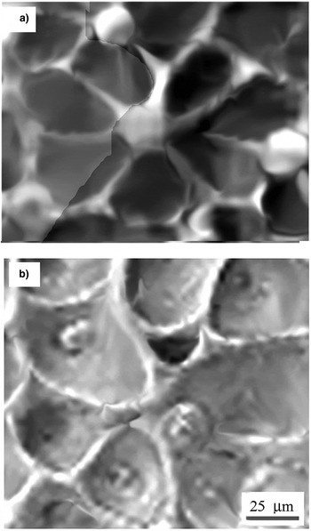
Fig. 11. The rosette-like web of horseshoe solitons with seven petals (bubble-cavities). (a) Scanning electron microscope (SEM) micrograph showing the rosette-like configuration of large bubbles. (b) SEM micrograph showing large bubbles “caged” by the horseshoe “walls” organized into the structure composed of two rosettes: one with three parabolic-like petals, and another with four petals.
The coherent flow field tends to establish the angular correlation of bubbles and organize them into 2D rosette–like web. The asymmetric rosette as a local structure in Figure 11a has a single center and seven petals, which are rather sharp near the center indicating triangular-like bubbles. The other domains comprise large ellipsoidal bubbles surrounded by the horseshoe “walls” organized into asymmetric rosette in the field of the short-range correlations (Fig. 11b). This structure has two slightly shifted centers, one with three and other with four petals, indicating the competition of the organization of two rosettes at the one and the same place. The lack of the long-range coherent flow field is the reason that 2D trigonal lattice is not established. Instead, the perturbation of correlation of bubble organization disturbs the translational and rotational symmetry indicating partially coherent flow field.
3.2.2.1. Horseshoe “walls” around bubbles: 2D horseshoe solitary waves
The horseshoe “walls” (Fig 11b) are the solidified waves, which preserve the parabolic-like contour known as the horseshoe solitons (as called by the mathematicians).Their characteristics are better seen in the domains comprising more simple cases like a single horseshoe soliton, two intersecting solitons, or the elliptic solitons. The profilometry of such structures in some cases reveals the vortex filaments formed by the rollup of the waves. These parabolic-like and the elliptic solitons can be simulated by using the cKP, or the ecKP equation, as shown by various mathematical groups (Klein et al., Reference Klein, Matveev and Smirnov2007; Li et al., Reference Li, Zhang, Xu, Zhang, Hu and Tian2007; Khusnutdinova et al., Reference Khusnutdinova, Klein, Matveev and Smirnov2013).
The SEM micrograph in Figure 12(i) shows a single horseshoe soliton, which can be reproduced by the one soliton solution of the cKP equation (Klein et al., Reference Klein, Matveev and Smirnov2007; Khusnutdinova et al., Reference Khusnutdinova, Klein, Matveev and Smirnov2013).

Fig. 12. Configurations of the horseshoe solitons. Scanning electron microscope (SEM) micrograph of the single parabolic-like soliton (i); SEM micrographs of two parabolic-like soliton crossings (i–iii).
The two horseshoe waves, which may interact by intersecting, merging, or splitting give rise to various configurations Figure 12(ii-iv). These configurations can be reproduced by the two soliton solution of cKP-I equation (where the gravity effects dominate), as seen in Figure 4 of Klein et al. (Reference Klein, Matveev and Smirnov2007).
Elliptic soliton configurations
Among the configurations of 2D nonlinear waves of the RMI turbulent mixing are the elliptic solitons, which are formed at the rim of elongated bubble-cavity. They appear either as one symmetric soliton (Fig. 13a), or the series of symmetric multisolitons (Fig. 13b). In the last case, two nearly-elliptic waves with the wavelength λ ~6–8 µm are of the lower intensity. Such elliptic symmetric solitons can be obtained by simulation based on ecKP-II equation (where the gravity effects dominate), as seen in Figure 17 of Khusnutdinova et al. (Reference Khusnutdinova, Klein, Matveev and Smirnov2013).

Fig. 13. Formation of elliptic solitary waves. (a) Scanning electron microscope (SEM) micrograph showing single elliptic solitary wave. (b) SEM micrograph showing three elliptic solitary waves.
4. CONCLUSION
The experiments have confirmed the hypothesis that the SCC causes formation of the new wave-vortex paradigm of 3D RMI turbulent mixing. The long lifetime of the hot vapor/plasma and fast reshocks at the megahertz scale establish the environment with more complex fluid dynamics of the wave-vortex phenomena.
The RMI morphology without spikes is generated by the high-pressure shock wave in the center of a Gaussian spot. Under condition (A ~1, P ~1.2 GPa, Re ~104–105), fast turbulent jet-spikes are broken up leaving only small remnants and the surface morphology with bubble-cavities.
The RMI environment is associated with the high-frequency reshocks, which couple with oscillation (pulsations) of bubbles in a random flow field and cause the separation of large nonspherical bubbles from the small spherical ones.
The strong influence of the oscillatory reshocks – depending on the parameters D and P – causes that bubble splitting, shape oscillations, merging, chaotic oscillations, and shape oscillations determine the bubble dynamics in turbulent mixing. Such bubble behavior generates the irregular wave front, which solidified makes the “walls” of variable shape and size (around the bubbles). The irregular cells connected into irregular – chaotic – web of (crumpled) broken “egg-karton” morphology, are characteristic for the random flow field. The bubbles, which in a flow field appear random regardless of whether or not there is forward energy cascade via vortex stretching down an inertial range – represent turbulent mixing. Development of a mixing layer with 3D turbulence at few spatial scales represents the statistically unsteady turbulent flow and stochastic process, which causes pressure pulsations and generates the self-similar structures. One can roughly assume that selfsimilarity at few spatial scales indicate turbulent mixing.
The RMI environment also has a strong influence on dynamics of bubbles in coherent flow field (which as a domain appears inside the random flow field). It comprises only the large bubbles showing narrow Gaussian-like number density distribution. The strong bubble-shape oscillation and collapse cause the formation of “wall” structures, around the bubbles actually the regular cells:
-
(i) The regular polygonal cells of the rhomb, square, and the pentagonal shape around the bubbles are the line solitary waves organized into the Voronoi web. The solitons as the nonlinear waves are caused by the strong bubble shape oscillations due to coupling with the oscillating force of the reshocks, and by the bubble collapse. The complex web of line solitons may be decomposed into local simple configurations like the resonant Y-type, nonresonant X-type, and triple-soliton junctions as well as quadruple-soliton junctions. These soliton configurations can be reproduced by the solutions of KP-II equation.
-
(ii) The regular horseshoe cells of the parabolic-like and the ellispoidal shape around the bubbles are the horseshoe solitons organized into the rosette-like web on trigonal lattice, but also into simple two-soliton crossings. These parabolic-like solitons can be reproduced by the solution of cKP- and the ecKP-equation.
The dominant morphology of the RMI in the SCC are the configurations of 2D solitary waves surrounding bubbles in the TMZ, which have overwhelmed the usual configurations of vortex pairing, merging, reconnection, splitting, and so on. The configurations of the line solitons and of the parabolic-like solitons – represent the new paradigm of the RMI turbulent mixing. The formation of solitary waves is a direct consequence of the strong nonlinear bubble shape oscillations forced by the high frequency filed of the reshocks in the semiconfined configuration.
SUPPLEMENTARY MATERIAL
The supplementary material for this article can be found at https://doi.org/10.1017/S0263034616000598
ACKNOWLEDGMENT
This work has been supported by the Croatian Science Foundation under the project: IP-2014-09-7046. The author is grateful to Prof. Y. Yanilkin and his colleagues, Russian Federation Nuclear Center-VNIIEF, Nizhniy Novgorod, Russia, for their papers and the results on the simulation of the RMI in the shock tube experiments, they kindly sent. The author is also grateful to Prof. N.J. Zabusky, Department of Physics of Complex Systems, Weizmann Institute of Science, Rehovot, Israel, particularly emphasizing the wave-vortex paradigm in turbulent mixing relating to the experiments. Finally, the author is grateful to the referee for valuable suggestions and comments, which improved the paper.


