2 The model

Our planar flow is incompressible and the boundary layer, lying on the wall $y^{\ast }=0$ with classical thickness $O(Re^{-1/2})$ , is laminar. The Reynolds number ( $Re$ ), taken to be large, is the ratio of inertial to viscous forces: $Re=U_{\infty }L/\unicode[STIX]{x1D708}$ , where $U_{\infty }$ is the speed of the oncoming flow, $L$ is a characteristic length scale and $\unicode[STIX]{x1D708}$ is the kinematic viscosity. Asterisked variables are non-dimensional, with dimensional equivalents given by $L(x^{\ast },y^{\ast })$ , $U_{\infty }(u^{\ast },v^{\ast })$ , $Lt^{\ast }/U_{\infty }$ and $\unicode[STIX]{x1D70C}U_{\infty }^{2}p^{\ast }$ , where $\unicode[STIX]{x1D70C}$ is the fluid density. As in SD, the flow encounters a hump, given by

(2.1) $$\begin{eqnarray}y^{\ast }=Re^{-1/2}\unicode[STIX]{x1D6FF}[hF(x^{\ast })+\hat{f}(h,x^{\ast },t^{\ast })],\end{eqnarray}$$

completely embedded within the classical boundary layer, with $Re^{-1/2}\unicode[STIX]{x1D6FF}$ the characteristic hump height (which, with $\unicode[STIX]{x1D6FF}\ll 1$ , is much smaller than the boundary-layer thickness) and $h$ the non-dimensional height factor of the bump. Here, $F$ is the hump shape, which achieves a maximum at $x^{\ast }=x_{max}^{\ast }$ , after which the pressure gradient becomes adverse and drives the flow towards separation. The additional contribution $\hat{f}$ corresponds to the roughness element, which is introduced in the region where the skin friction vanishes (see § 2.2) but is identically zero everywhere else. Its crucial height scale, which is some power of $h$ , will be determined later. Finally, the streamwise coordinate $x^{\ast }$ and time $t^{\ast }$ are based on the non-dimensional length scale of the bump, which in turn is based on the Reynolds number as shown in (2.2).

As mentioned in the introduction, the local separation point coincides with the position of zero skin friction and the appearance of the Goldstein singularity but, as demonstrated by SD, this singularity is moved downstream and eventually removed completely. This is through physical interactions in different flow regions (see below), and is seen most readily when the characteristic length ( $\ell$ ) and height scales of the hump satisfy $Re^{-3/4}\ll \ell \ll Re^{-3/8}$ and $Re^{-1/4}\ll \unicode[STIX]{x1D6FF}\ll Re^{-1/8}$ (Smith et al. Reference Smith, Brighton, Jackson and Hunt1981). Then the coordinates and variables scale as

(2.2a-c ) $$\begin{eqnarray}\displaystyle x^{\ast }=\ell x,\quad y^{\ast }=Re^{-1/2}\ell ^{1/3}(y+hF+\hat{f}),\quad t^{\ast }=\ell ^{2/3}t, & & \displaystyle\end{eqnarray}$$

(2.2d-f ) $$\begin{eqnarray}\displaystyle p^{\ast }=\ell ^{2/3}p,\quad u^{\ast }=\ell ^{1/3}u,\quad v^{\ast }=Re^{-1/2}\ell ^{-1/3}\left[v+\frac{\unicode[STIX]{x2202}\hat{f}}{\unicode[STIX]{x2202}t}+u\frac{\unicode[STIX]{x2202}}{\unicode[STIX]{x2202}x}(hF+\hat{f})\right],\qquad & & \displaystyle\end{eqnarray}$$

with all unasterisked quantities of $O(1)$ , where a Prandtl transposition has been applied to simplify the no-slip condition of (2.4). Substituting into the Navier–Stokes equations, we obtain, written in terms of the streamfunction $\unicode[STIX]{x1D713}$ , the unsteady condensed-flow equations

(2.3a-c ) $$\begin{eqnarray}u=\frac{\unicode[STIX]{x2202}\unicode[STIX]{x1D713}}{\unicode[STIX]{x2202}y},\quad v=-\frac{\unicode[STIX]{x2202}\unicode[STIX]{x1D713}}{\unicode[STIX]{x2202}x},\quad \frac{\unicode[STIX]{x2202}^{2}\unicode[STIX]{x1D713}}{\unicode[STIX]{x2202}y\unicode[STIX]{x2202}t}+\frac{\unicode[STIX]{x2202}\unicode[STIX]{x1D713}}{\unicode[STIX]{x2202}y}\frac{\unicode[STIX]{x2202}^{2}\unicode[STIX]{x1D713}}{\unicode[STIX]{x2202}x\unicode[STIX]{x2202}y}-\frac{\unicode[STIX]{x2202}\unicode[STIX]{x1D713}}{\unicode[STIX]{x2202}x}\frac{\unicode[STIX]{x2202}^{2}\unicode[STIX]{x1D713}}{\unicode[STIX]{x2202}y^{2}}=-\frac{\unicode[STIX]{x2202}p}{\unicode[STIX]{x2202}x}(x,t)+\frac{\unicode[STIX]{x2202}^{3}\unicode[STIX]{x1D713}}{\unicode[STIX]{x2202}y^{3}}.\end{eqnarray}$$

These are subject to the boundary conditions

(2.4a ) $$\begin{eqnarray}\displaystyle \unicode[STIX]{x1D713}=\frac{\unicode[STIX]{x2202}\unicode[STIX]{x1D713}}{\unicode[STIX]{x2202}y}=0\quad \text{on }y=0, & & \displaystyle\end{eqnarray}$$

(2.4b,c ) $$\begin{eqnarray}\displaystyle \unicode[STIX]{x1D713}\rightarrow {\textstyle \frac{1}{2}}y^{2},\quad p\rightarrow 0\quad \text{as }x\rightarrow -\infty , & & \displaystyle\end{eqnarray}$$

(2.4d ) $$\begin{eqnarray}\displaystyle u\sim y+hF(x)+\hat{f}(h,x,t)\quad \text{as }y\rightarrow \infty , & & \displaystyle\end{eqnarray}$$

corresponding to no slip, matching with the boundary layer far upstream and the requirement that there be no displacement of the original boundary layer and outer inviscid flow due to the presence of the (relatively) small hump. We note that this system is valid for all values of the non-dimensional hump height ( $h$ ) strictly between zero and infinity, provided that $h\ll \unicode[STIX]{x1D6FF}^{-1}Re^{-1/8}$ (for example, for bumps with a length scale equal to the boundary-layer height, $\ell \sim Re^{-1/2}$ , one obtains a bump height scale $\unicode[STIX]{x1D6FF}\sim \ell ^{1/3}\sim Re^{-1/6}$ ; and hence $h\ll Re^{1/24}$ ), and we will focus here on cases where $h\gg 1$ , as per the work of Smith & Daniels (Reference Smith and Daniels1981): small $h$ , albeit without dynamic roughness, was studied by Smith (Reference Smith1976b ), while situations where $h=O(1)$ appear in Smith (Reference Smith1976a ).

2.1 The flow development

The development of the flow can be divided into the following regions: the flow upstream of the hump and over its front face is attached and can be dealt with using classical boundary-layer theory (region A in figure 1); this classical approach breaks down as the Goldstein singularity is approached at the rear of the hump, and the singularity can be shifted downstream by considering a smaller length scale around the singular point (region B), with the boundary layer split vertically into two sublayers; the singularity can then be removed completely by considering a still smaller length scale, allowing the skin friction to pass smoothly through zero (region C); complete nonlinear breakaway of the near-wall layer, associated with the presence of a (removable) singularity in region C, occurs in a fourth region (D), upstream of the separated flow (E) reattaching further downstream. Our interest is mainly in the positions of zero skin friction (§§ 3 and 4) and the removable singularity appearing downstream of it (§ 5), both of which occur in region C, which is where the roughness element will be placed. In this section, we summarise the solutions to the streamfunctions and pressures in regions A and B, before focusing on region C in the next section. The effect of the roughness is expected to be mostly local and thus for the flow in regions D and E, we refer the reader to the SD paper.

Figure 1. The development of the flow in the ( $x,y$ )-plane as it reaches the Goldstein singularity at the end of region A and proceeds downstream. A summary of each flow region is given in the text; the dynamic roughness (grey) is placed in region C, which has a length scale of $O(h^{-3/2})$ . Not to scale.

The steady flow upstream of the Goldstein singularity consists of a viscous near-wall region of vertical scale $O(h^{-1/2})$ and a large inviscid outer zone where $y=O(h)$ . The boundary condition at infinity sets the form of the streamfunction in the outer layer; imposing the condition of no normal flow at $y=0$ in the outer layer solution gives the leading-order pressure term, which drives the leading-order flow in the viscous sublayer. Matching determines the next term in the pressure expansion, and so on. The outer layer streamfunction is then

(2.5) $$\begin{eqnarray}\unicode[STIX]{x1D713}={\textstyle \frac{1}{2}}[y+hF(x)]^{2}+p\end{eqnarray}$$

and the viscous layer streamfunction responds as

(2.6) $$\begin{eqnarray}\unicode[STIX]{x1D713}\sim h^{1/2}F(x)[Y-\unicode[STIX]{x1D6FD}_{0}(x)]+h^{-1}\left[{\textstyle \frac{1}{2}}Y^{2}+p_{2}(x)\right]+\cdots\end{eqnarray}$$

as $Y\rightarrow \infty$ , with a pressure expansion of

(2.7) $$\begin{eqnarray}p=-{\textstyle \frac{1}{2}}h^{2}F^{2}(x)-h^{1/2}\unicode[STIX]{x1D6FD}_{0}(x)F(x)+\cdots \,.\end{eqnarray}$$

Here, $Y$ is the scaled normal coordinate in the inner layer, given by $y=h^{-1/2}Y$ , and $\unicode[STIX]{x1D6FD}_{0}(x)$ is obtained from the numerical solution to the classical boundary-layer equations obtained in that layer.

Denoting by $x_{s}$ the position at which the scaled skin friction ( $\unicode[STIX]{x1D70F}_{wall}\equiv \unicode[STIX]{x2202}^{2}\unicode[STIX]{x1D713}/\unicode[STIX]{x2202}y^{2}$ evaluated at $y=0$ ) vanishes, Goldstein (Reference Goldstein1948) showed that the above procedure first outlined by Prandtl gives rise to a square-root singularity as $x$ approaches $x_{s}$ . If we look at the limit as $x\rightarrow x_{s}^{-}$ , the viscous layer splits into two decks: an outer Goldstein layer, where $Y$ remains of $O(1)$ ; and an inner Goldstein layer, where the vertical coordinate is scaled as $\unicode[STIX]{x1D702}=Y(x_{s}-x)^{-1/4}\sim 1$ . The streamfunction in the inner Goldstein layer then behaves as

(2.8) $$\begin{eqnarray}\unicode[STIX]{x1D713}^{i}=h^{1/2}\left[{\textstyle \frac{1}{6}}\unicode[STIX]{x1D707}(x_{s}-x)^{3/4}\unicode[STIX]{x1D702}^{3}+\unicode[STIX]{x1D6FC}_{0}(x_{s}-x)\unicode[STIX]{x1D702}^{2}+(x_{s}-x)^{5/4}\left(\unicode[STIX]{x1D6FC}_{1}\unicode[STIX]{x1D702}^{2}-{\textstyle \frac{1}{60}}\unicode[STIX]{x1D6FC}_{0}^{2}\unicode[STIX]{x1D702}^{5}\right)\right]+\cdots \,,\end{eqnarray}$$

from which one can identify the square-root singularity in $\unicode[STIX]{x1D70F}_{wall}$ . Here $\unicode[STIX]{x1D707}=-F_{s}F_{s}^{\prime }>0$ , where $F_{s}=F(x_{s})$ ; and $\unicode[STIX]{x1D6FC}_{0}$ and $\unicode[STIX]{x1D6FC}_{1}\propto \unicode[STIX]{x1D6FC}_{0}^{2}$ are unknown, non-zero positive constants. The outer Goldstein layer streamfunction can be represented as

(2.9) $$\begin{eqnarray}\unicode[STIX]{x1D713}^{o}=h^{1/2}\left[\unicode[STIX]{x1D713}_{0s}(Y)+\frac{2\unicode[STIX]{x1D6FC}_{0}}{\unicode[STIX]{x1D707}}(x_{s}-x)^{1/2}\unicode[STIX]{x1D713}_{0s}^{\prime }(Y)+\frac{2\unicode[STIX]{x1D6FC}_{1}}{\unicode[STIX]{x1D707}}(x_{s}-x)^{3/4}\unicode[STIX]{x1D713}_{0s}^{\prime }(Y)\right]+\cdots \,,\end{eqnarray}$$

where

(2.10) $$\begin{eqnarray}\left.\begin{array}{@{}c@{}}\displaystyle \unicode[STIX]{x1D713}_{0s}(Y)\sim {\textstyle \frac{1}{6}}\unicode[STIX]{x1D707}Y^{3}-{\textstyle \frac{1}{60}}\unicode[STIX]{x1D6FC}_{0}^{2}Y^{5}+\cdots \quad \text{as }Y\rightarrow 0,\\ \displaystyle \unicode[STIX]{x1D713}_{0s}(Y)\sim F_{s}(Y-\unicode[STIX]{x1D6FD}_{s})+o(1)\quad \text{as }Y\rightarrow \infty ,\end{array}\right\}\end{eqnarray}$$

with $\unicode[STIX]{x1D6FD}_{s}=\unicode[STIX]{x1D6FD}(x_{s})$ being constant.

Removal of the Goldstein singularity begins over the length scale $x-x_{s}\sim h^{-3/2}\ln h$ of region B. The outer Goldstein layer retains the height scale $Y\sim 1$ , while the inner Goldstein layer has $Y=h^{-3/8}(\ln h)^{1/4}\bar{z}$ and we introduce the new streamwise coordinate $x-x_{s}=h^{-3/2}\ln (h)\bar{X}$ ; $\bar{X},\bar{z}\sim 1$ . The relevant streamfunctions (SD) are then

(2.11a ) $$\begin{eqnarray}\displaystyle \bar{\unicode[STIX]{x1D713}}^{o} & = & \displaystyle h^{1/2}\unicode[STIX]{x1D713}_{0s}(Y)+\unicode[STIX]{x1D713}_{0s}^{\prime }(Y)\left[h^{-1/4}(\ln h)^{1/2}\bar{\unicode[STIX]{x1D6FC}}_{1}(\bar{X})\right.\nonumber\\ \displaystyle & & \displaystyle \left.+\,h^{-1/4}(\ln h)^{-1/2}\ln (\ln h)\bar{\unicode[STIX]{x1D6FC}}_{1L}(\bar{X})+h^{-1/4}(\ln h)^{-1/2}\bar{\unicode[STIX]{x1D6FC}}_{2}(\bar{X})\right]+\cdots \,,\end{eqnarray}$$

(2.11b ) $$\begin{eqnarray}\displaystyle \bar{\unicode[STIX]{x1D713}}^{i} & = & \displaystyle h^{-5/8}(\ln h)^{3/4}\left({\textstyle \frac{1}{6}}\unicode[STIX]{x1D707}\bar{z}^{3}\right)+\left({\textstyle \frac{1}{2}}\unicode[STIX]{x1D707}\bar{z}^{2}\right)\left[h^{-1}(\ln h)\bar{\unicode[STIX]{x1D6FC}}_{1}(\bar{X})+h^{-1}\ln (\ln h)\bar{\unicode[STIX]{x1D6FC}}_{1L}(\bar{X})\right.\nonumber\\ \displaystyle & & \displaystyle \left.+\,h^{-1}\bar{\unicode[STIX]{x1D6FC}}_{2}(\bar{X})\right]+h^{-11/8}(\ln h)^{5/4}\left({\textstyle \frac{1}{2}}\unicode[STIX]{x1D707}\bar{z}^{2}\bar{\unicode[STIX]{x1D6FC}}_{3}(\bar{X})-{\textstyle \frac{1}{60}}\unicode[STIX]{x1D6FC}_{0}^{2}\bar{z}^{5}\right)+\cdots\end{eqnarray}$$

for the outer and inner Goldstein layers respectively, and

(2.12) $$\begin{eqnarray}\displaystyle p & = & \displaystyle h^{2}\left(-{\textstyle \frac{1}{2}}F_{s}^{2}\right)+h^{1/2}\ln h(\unicode[STIX]{x1D707}\bar{X})+h^{1/2}(-\unicode[STIX]{x1D6FD}_{s}F_{s})+F_{s}\left[h^{-1/4}(\ln h)^{1/2}\bar{\unicode[STIX]{x1D6FC}}_{1}(\bar{X})\right.\nonumber\\ \displaystyle & & \displaystyle \left.+\,h^{-1/4}(\ln h)^{-1/2}\ln (\ln h)\bar{\unicode[STIX]{x1D6FC}}_{1L}(\bar{X})+h^{-1/4}(\ln h)^{-1/2}\bar{\unicode[STIX]{x1D6FC}}_{2}(\bar{X})\right]+\cdots\end{eqnarray}$$

for the pressure; also

(2.13a ) $$\begin{eqnarray}\displaystyle & \displaystyle \bar{\unicode[STIX]{x1D6FC}}_{1}(\bar{X})=2\unicode[STIX]{x1D707}^{-1}\unicode[STIX]{x1D6FC}_{0}\left(-\bar{X}+\frac{3A_{0L}}{2\unicode[STIX]{x1D6FC}_{0}}\right)^{1/2}, & \displaystyle\end{eqnarray}$$

(2.13b ) $$\begin{eqnarray}\displaystyle & \displaystyle \bar{\unicode[STIX]{x1D6FC}}_{1L}(\bar{X})=-\unicode[STIX]{x1D707}^{-1}A_{0L}\left(-\bar{X}+\frac{3A_{0L}}{2\unicode[STIX]{x1D6FC}_{0}}\right)^{-1/2}, & \displaystyle\end{eqnarray}$$

(2.13c ) $$\begin{eqnarray}\displaystyle \bar{\unicode[STIX]{x1D6FC}}_{2}(\bar{X}) & = & \displaystyle -\unicode[STIX]{x1D707}^{-1}A_{0L}\left(-\bar{X}+\frac{3A_{0L}}{2\unicode[STIX]{x1D6FC}_{0}}\right)^{-1/2}\ln \left(-\bar{X}+\frac{3A_{0L}}{2\unicode[STIX]{x1D6FC}_{0}}\right)\nonumber\\ \displaystyle & & \displaystyle +\,\unicode[STIX]{x1D707}^{-1}A_{0}\left(-\bar{X}+\frac{3A_{0L}}{2\unicode[STIX]{x1D6FC}_{0}}\right)^{-1/2},\end{eqnarray}$$

(2.13d ) $$\begin{eqnarray}\displaystyle A_{0L}=\frac{F_{s}\left(-\frac{1}{4}\right)!}{2^{5/2}\unicode[STIX]{x1D707}^{1/2}\left(\frac{1}{4}\right)!}, & & \displaystyle\end{eqnarray}$$

and $\bar{\unicode[STIX]{x1D6FC}}_{3}$ , $A_{0}$ are associated functions and constants.

The above expansions result in a scaled skin friction of

(2.14) $$\begin{eqnarray}\unicode[STIX]{x1D70F}_{wall}=2\unicode[STIX]{x1D6FC}_{0}h^{3/4}(\ln h)^{1/2}\left(-\bar{X}+\frac{3A_{0L}}{2\unicode[STIX]{x1D6FC}_{0}}\right)^{1/2}+\cdots \,,\end{eqnarray}$$

indicating that the Goldstein singularity has merely been shifted to the position $\bar{X}=3A_{0L}/2\unicode[STIX]{x1D6FC}_{0}$ . Its complete removal, as well as the introduction of the dynamic roughness, is considered in the following section.

2.2 The roughness region

As $\bar{X}$ approaches $3A_{0L}/2\unicode[STIX]{x1D6FC}_{0}$ , the streamfunction expansion in the inner Goldstein layer (2.11b ) breaks down. In particular, this occurs when

(2.15) $$\begin{eqnarray}\left(-\bar{X}+\frac{3A_{0L}}{2\unicode[STIX]{x1D6FC}_{0}}\right)\sim (\ln h)^{-1}.\end{eqnarray}$$

We therefore define coordinates $(X,z)$ in the inner and $(X,Y)$ in the outer Goldstein layers, all of $O(1)$ , as

(2.16a-c ) $$\begin{eqnarray}x-x_{s}=h^{-3/2}\ln (h)\frac{3A_{0L}}{2\unicode[STIX]{x1D6FC}_{0}}+h^{-3/2}X,\quad y=h^{-7/8}z,\quad \text{and}\quad y=h^{-1/2}Y.\end{eqnarray}$$

It is in this region that we introduce the roughness element in order to investigate the impact it has both on the position of zero skin friction and downstream singularity. For the purposes of the following derivation, we will take the roughness element to be time dependent, although static elements will also be studied in §§ 3 and 5. At the former position, $\unicode[STIX]{x1D70F}_{wall}$ will pass regularly through zero, while the latter is also removable in a physically sensible fashion in region D and corresponds to the full nonlinear breakaway of the boundary layer (SD). The height scale of the roughness element is $O(h^{-5/4})$ and the oscillation frequency is of order $h^{11/8}$ , indicating the scaled time

(2.17) $$\begin{eqnarray}T=h^{11/8}t:\end{eqnarray}$$

these scalings affect the governing equations at the appropriate order, but other possible choices will be referred to at the end of this section.

The boundary condition at infinity, (2.4d ), can be integrated with respect to $y$ to obtain the streamfunction behaviour

(2.18) $$\begin{eqnarray}\unicode[STIX]{x1D713}\sim {\textstyle \frac{1}{2}}[y+hF(x)+h^{-5/4}f(x,T)]^{2}+q(x,T)\quad \text{as }y\rightarrow \infty ,\end{eqnarray}$$

where $\hat{f}=h^{-5/4}f$ . The function $q$ is determined by taking the limit of the condensed-flow equation (2.3c ) as $y\rightarrow \infty$ and gives

(2.19) $$\begin{eqnarray}q(x,T)=p(x,T)+h^{1/8}\int _{-\infty }^{x}\frac{\unicode[STIX]{x2202}f}{\unicode[STIX]{x2202}T}(s,T)\,\text{d}s.\end{eqnarray}$$

Thus the streamfunction behaves as

(2.20) $$\begin{eqnarray}\unicode[STIX]{x1D713}\sim \frac{1}{2}[y+hF(x)+h^{-5/4}f(x,T)]^{2}+p(x,T)+h^{1/8}\int _{-\infty }^{x}\frac{\unicode[STIX]{x2202}f}{\unicode[STIX]{x2202}T}(s,T)\,\text{d}s\end{eqnarray}$$

when $y\rightarrow \infty$ . Note that the above is valid throughout the streamwise extent of the hump, $x\sim 1$ , under the understanding that $f$ is identically zero everywhere outside the small roughness region defined above. Thus there is no contradiction with the previous equation (2.5).

The form of the pressure in this region is derived from the upstream pressure (2.12), which is rewritten using the new streamwise coordinate $X$ to suggest the expansion

(2.21) $$\begin{eqnarray}p(X,T)=-h^{2}\left(\frac{1}{2}F_{s}^{2}\right)+h^{1/2}(\ln h)\frac{3A_{0L}}{2\unicode[STIX]{x1D6FC}_{0}}\unicode[STIX]{x1D707}+h^{1/2}(\unicode[STIX]{x1D707}\bar{X}-\unicode[STIX]{x1D6FD}_{s}F_{s})+h^{-1/4}P_{1}+\cdots \,.\end{eqnarray}$$

The streamfunction in the outer Goldstein layer must match with that of (2.20) as $Y\rightarrow \infty$ ; and thus expanding the latter about $x_{s}$ and rewriting it in terms of the normal coordinate $Y$ , provides the expansion

(2.22) $$\begin{eqnarray}\unicode[STIX]{x1D6F9}^{o}(X,Y,T)=h^{1/2}\unicode[STIX]{x1D6F9}_{1}^{o}(X,Y,T)+h^{-1/4}\unicode[STIX]{x1D6F9}_{2}^{o}(X,Y,T)+\cdots \,,\end{eqnarray}$$

with the functions $\unicode[STIX]{x1D6F9}_{i}^{o}$ satisfying the matching conditions

(2.23a ) $$\begin{eqnarray}\displaystyle & \displaystyle \unicode[STIX]{x1D6F9}_{1}^{o}\rightarrow F_{s}(Y-\unicode[STIX]{x1D6FD}_{s})\quad \text{as }Y\rightarrow \infty , & \displaystyle\end{eqnarray}$$

(2.23b ) $$\begin{eqnarray}\displaystyle & \displaystyle \unicode[STIX]{x1D6F9}_{1}^{o}\rightarrow \unicode[STIX]{x1D713}_{0s}(Y)\quad \text{as }X\rightarrow -\infty , & \displaystyle\end{eqnarray}$$

(2.23c ) $$\begin{eqnarray}\displaystyle & \displaystyle \unicode[STIX]{x1D6F9}_{2}^{o}\rightarrow P_{1}(X,T)+F_{s}\,f(X,T)\quad \text{as }Y\rightarrow \infty , & \displaystyle\end{eqnarray}$$

(2.23d ) $$\begin{eqnarray}\displaystyle & \displaystyle \unicode[STIX]{x1D6F9}_{2}^{o}\rightarrow 2\unicode[STIX]{x1D707}^{-1}\unicode[STIX]{x1D6FC}_{0}\unicode[STIX]{x1D713}_{0s}^{\prime }(Y)|X|^{1/2}+\cdots \quad \text{as }X\rightarrow -\infty ; & \displaystyle\end{eqnarray}$$

the upstream conditions here arise from (2.11a ).

Substitution of the expansions (2.21) and (2.22) into the condensed flow equation (2.3) gives the governing equations for the components $\unicode[STIX]{x1D6F9}_{i}^{o}$ , solved subject to the matching conditions (2.23) above. Thus the equation

(2.24) $$\begin{eqnarray}\frac{\unicode[STIX]{x2202}\unicode[STIX]{x1D6F9}_{1}^{o}}{\unicode[STIX]{x2202}Y}\frac{\unicode[STIX]{x2202}^{2}\unicode[STIX]{x1D6F9}_{1}^{o}}{\unicode[STIX]{x2202}X\unicode[STIX]{x2202}Y}-\frac{\unicode[STIX]{x2202}\unicode[STIX]{x1D6F9}_{1}^{o}}{\unicode[STIX]{x2202}X}\frac{\unicode[STIX]{x2202}^{2}\unicode[STIX]{x1D6F9}_{1}^{o}}{\unicode[STIX]{x2202}Y^{2}}=0\end{eqnarray}$$

for $\unicode[STIX]{x1D6F9}_{1}^{o}$ is solved to obtain

(2.25) $$\begin{eqnarray}\unicode[STIX]{x1D6F9}_{1}^{o}=\unicode[STIX]{x1D713}_{0s}(Y);\end{eqnarray}$$

and

(2.26) $$\begin{eqnarray}\unicode[STIX]{x1D713}_{0s}^{\prime }\frac{\unicode[STIX]{x2202}^{2}\unicode[STIX]{x1D6F9}_{2}^{o}}{\unicode[STIX]{x2202}X\unicode[STIX]{x2202}Y}-\unicode[STIX]{x1D713}_{0s}^{\prime \prime }\frac{\unicode[STIX]{x2202}\unicode[STIX]{x1D6F9}_{2}^{o}}{\unicode[STIX]{x2202}X}=0,\end{eqnarray}$$

for

(2.27) $$\begin{eqnarray}\unicode[STIX]{x1D6F9}_{2}^{o}=\unicode[STIX]{x1D713}_{0s}^{\prime }(Y)[A(X,T)+f(X,T)],\end{eqnarray}$$

using the properties of $\unicode[STIX]{x1D713}_{0s}$ given in (2.10). Hence

(2.28) $$\begin{eqnarray}\unicode[STIX]{x1D6F9}^{o}=h^{1/2}\unicode[STIX]{x1D713}_{0s}(Y)+h^{-1/4}\unicode[STIX]{x1D713}_{0s}^{\prime }(Y)[A(X,T)+f(X,T)]+\cdots\end{eqnarray}$$

is the streamfunction to the first two orders in the outer Goldstein layer. Terms at orders $h^{-1}$ and $h^{-11/8}$ also affect the inner layer expansion of (2.30) below.

The displacement function $A$ is related to the pressure through the pressure–displacement relation

(2.29) $$\begin{eqnarray}P_{1}=F_{s}A,\end{eqnarray}$$

on applying the condition (2.23c ). This displacement function must be found by considering the flow in the inner Goldstein layer and thus the outer layer causes interaction between the viscous flow in the layer very near the wall and the bulk of the flow in the main boundary layer. The displacement $A$ also appears in the expression for the wall skin friction and thus its determination is the main focus of the remainder of this section.

Turning therefore to the inner Goldstein layer, the streamfunction expansion is once again found by rewriting the oncoming streamfunction (2.11b ) in terms of the $(X,z)$ coordinate system of our region of interest. This gives

(2.30) $$\begin{eqnarray}\unicode[STIX]{x1D6F9}^{i}(X,z,T)=h^{-5/8}\unicode[STIX]{x1D6F9}_{1}^{i}(X,z,T)+h^{-1}\unicode[STIX]{x1D6F9}_{2}^{i}(X,z,T)+h^{-11/8}\unicode[STIX]{x1D6F9}_{3}^{i}(X,z,T)+\cdots \,,\end{eqnarray}$$

an expansion that is confirmed by rewriting (2.28) as $Y\rightarrow 0$ using $Y=h^{-3/8}z$ . The condensed-flow equation (2.3) in the inner Goldstein layer of the roughness region is

(2.31) $$\begin{eqnarray}h^{9/4}\frac{\unicode[STIX]{x2202}^{2}\unicode[STIX]{x1D6F9}^{i}}{\unicode[STIX]{x2202}T\unicode[STIX]{x2202}z}+h^{13/4}\frac{\unicode[STIX]{x2202}\unicode[STIX]{x1D6F9}^{i}}{\unicode[STIX]{x2202}z}\frac{\unicode[STIX]{x2202}^{2}\unicode[STIX]{x1D6F9}^{i}}{\unicode[STIX]{x2202}X\unicode[STIX]{x2202}z}-h^{13/4}\frac{\unicode[STIX]{x2202}\unicode[STIX]{x1D6F9}^{i}}{\unicode[STIX]{x2202}X}\frac{\unicode[STIX]{x2202}^{2}\unicode[STIX]{x1D6F9}^{i}}{\unicode[STIX]{x2202}z^{2}}=-h^{3/2}\frac{\unicode[STIX]{x2202}p}{\unicode[STIX]{x2202}X}+h^{21/8}\frac{\unicode[STIX]{x2202}^{3}\unicode[STIX]{x1D6F9}^{i}}{\unicode[STIX]{x2202}z^{3}},\end{eqnarray}$$

into which we substitute the expansions (2.30) and (2.21). Each order is then equated to form a governing equation for the terms in the expansion, to which we apply the no-slip boundary condition, matching with the upstream streamfunction and the outer Goldstein layer. The first two terms are

(2.32a ) $$\begin{eqnarray}\displaystyle & \displaystyle \unicode[STIX]{x1D6F9}_{1}^{i}(X,z,T)={\textstyle \frac{1}{6}}\unicode[STIX]{x1D707}z^{3}, & \displaystyle\end{eqnarray}$$

(2.32b ) $$\begin{eqnarray}\displaystyle & \displaystyle \unicode[STIX]{x1D6F9}_{2}^{i}(X,z,T)={\textstyle \frac{1}{2}}\unicode[STIX]{x1D707}z^{2}[A(X,T)+f(X,T)], & \displaystyle\end{eqnarray}$$

with the second-order system also yielding the upstream condition on the displacement function $A$ ,

(2.33) $$\begin{eqnarray}A(X,T)\rightarrow 2\unicode[STIX]{x1D707}^{-1}\unicode[STIX]{x1D6FC}_{0}|X|^{1/2}-\unicode[STIX]{x1D707}^{-1}A_{0L}|X|^{-1/2}\ln |X|+\unicode[STIX]{x1D707}^{-1}A_{0}|X|^{-1/2}\end{eqnarray}$$

as $X\rightarrow -\infty$ .

Comparing these with the results of SD, we see that the solution at leading order is the same, with the solution to $\unicode[STIX]{x1D6F9}_{2}^{i}$ (their $\bar{\unicode[STIX]{x1D713}}_{1}$ ) being modified by the addition of $f$ . The wall skin friction is then

(2.34) $$\begin{eqnarray}\unicode[STIX]{x1D70F}_{wall}(X,T)=h^{3/4}\unicode[STIX]{x1D707}(A+f)+\cdots\end{eqnarray}$$

to leading order and thus we are interested in the streamwise position where

(2.35) $$\begin{eqnarray}A(X,T)+f(X,T)=0.\end{eqnarray}$$

The displacement function $A$ is found through the governing equation for $\unicode[STIX]{x1D6F9}_{3}^{i}$ , which is

(2.36) $$\begin{eqnarray}\frac{\unicode[STIX]{x2202}^{3}\unicode[STIX]{x1D6F9}_{3}^{i}}{\unicode[STIX]{x2202}z^{3}}+\unicode[STIX]{x1D707}z\frac{\unicode[STIX]{x2202}\unicode[STIX]{x1D6F9}_{3}^{i}}{\unicode[STIX]{x2202}X}-\frac{1}{2}\unicode[STIX]{x1D707}z^{2}\frac{\unicode[STIX]{x2202}^{2}\unicode[STIX]{x1D6F9}_{3}^{i}}{\unicode[STIX]{x2202}X\unicode[STIX]{x2202}z}=\frac{\unicode[STIX]{x2202}P_{1}}{\unicode[STIX]{x2202}X}+\frac{1}{2}\unicode[STIX]{x1D707}z^{2}(A+f)\frac{\unicode[STIX]{x2202}}{\unicode[STIX]{x2202}X}(A+f)+\unicode[STIX]{x1D707}z\frac{\unicode[STIX]{x2202}}{\unicode[STIX]{x2202}T}(A+f),\end{eqnarray}$$

to be solved subject to the condition of no slip, upstream matching and the condition as $z\rightarrow \infty$ that

(2.37) $$\begin{eqnarray}\unicode[STIX]{x1D6F9}_{3}^{i}\rightarrow -\frac{1}{60}\unicode[STIX]{x1D6FC}_{0}^{2}z^{5}+\frac{1}{2}A_{2}z^{2}+\frac{1}{2}\unicode[STIX]{x1D707}(A+f)^{2}z+\int _{-\infty }^{X}\frac{\unicode[STIX]{x2202}}{\unicode[STIX]{x2202}T}(A+f)\,\text{d}X,\end{eqnarray}$$

where the function $A_{2}$ is unknown. A similar approach to that carried out by SD, Stewartson (Reference Stewartson1970), Ruban (Reference Ruban1981, Reference Ruban1982), Smith (Reference Smith1982), Stewartson et al. (Reference Stewartson, Smith and Kaups1982), BK and Braun & Scheichl (Reference Braun and Scheichl2014) yields the governing equation for the displacement $A$ :

(2.38) $$\begin{eqnarray}\displaystyle & & \displaystyle (A+f)\frac{\unicode[STIX]{x2202}}{\unicode[STIX]{x2202}X}(A+f)+\unicode[STIX]{x1D70E}_{1}\int _{-\infty }^{X}(X-s)^{-1/4}\frac{\unicode[STIX]{x2202}^{2}}{\unicode[STIX]{x2202}T\unicode[STIX]{x2202}s}(A+f)\,\text{d}s+2\unicode[STIX]{x1D707}^{-2}\unicode[STIX]{x1D6FC}_{0}^{2}\nonumber\\ \displaystyle & & \displaystyle \qquad =-\unicode[STIX]{x1D70E}_{2}F_{s}\int _{-\infty }^{X}(X-s)^{-1/2}\frac{\unicode[STIX]{x2202}^{2}A}{\unicode[STIX]{x2202}s^{2}}\,\text{d}s,\end{eqnarray}$$

subject to the starting condition (2.33). In the above, we have already made use of the pressure–displacement relation (2.29) to obtain the integral term on the right-hand side and $\unicode[STIX]{x1D70E}_{1}$ , $\unicode[STIX]{x1D70E}_{2}$ are constants given by

(2.39a,b ) $$\begin{eqnarray}\unicode[STIX]{x1D70E}_{1}=2^{5/4}\unicode[STIX]{x03C0}^{-1}\unicode[STIX]{x1D707}^{-3/4}\left(-{\textstyle \frac{1}{4}}\right)!\quad \text{and }\quad \unicode[STIX]{x1D70E}_{2}=\unicode[STIX]{x03C0}^{-1}\unicode[STIX]{x1D707}^{-3/2}\left[\left(-{\textstyle \frac{1}{4}}\right)!\right]^{2},\end{eqnarray}$$

both positive.

The affine transformation

(2.40a-c ) $$\begin{eqnarray}A=(2\unicode[STIX]{x1D6FC}_{0}\unicode[STIX]{x1D70E}_{2}\unicode[STIX]{x1D707}^{-1}F_{s})^{1/2}\hat{A},\quad f=(2\unicode[STIX]{x1D6FC}_{0}\unicode[STIX]{x1D70E}_{2}\unicode[STIX]{x1D707}^{-1}F_{s})^{1/2}\hat{f},\quad T={\textstyle \frac{1}{2}}\unicode[STIX]{x1D707}\unicode[STIX]{x1D6FC}_{0}^{-1}\unicode[STIX]{x1D70E}_{1}\left({\textstyle \frac{1}{2}}\unicode[STIX]{x1D707}\unicode[STIX]{x1D6FC}_{0}^{-1}\unicode[STIX]{x1D70E}_{2}F_{s}\right)^{1/4}\hat{T}\end{eqnarray}$$

(2.41) $$\begin{eqnarray}X={\textstyle \frac{1}{2}}\unicode[STIX]{x1D707}\unicode[STIX]{x1D6FC}_{0}^{-1}\unicode[STIX]{x1D70E}_{2}F_{s}\left\{\hat{X}-2(\unicode[STIX]{x1D707}\unicode[STIX]{x1D70E}_{2}F_{s})^{-1}\left[\unicode[STIX]{x1D6FC}_{0}-A_{0L}\ln \left({\textstyle \frac{1}{2}}\unicode[STIX]{x1D707}\unicode[STIX]{x1D6FC}_{0}^{-1}\unicode[STIX]{x1D70E}_{2}F_{s}\right)\right]\right\},\end{eqnarray}$$

takes the above equation for $A$ to (removing the overhat)

(2.42) $$\begin{eqnarray}(A+f)\frac{\unicode[STIX]{x2202}}{\unicode[STIX]{x2202}X}(A+f)+\int _{-\infty }^{X}(X-s)^{-1/4}\frac{\unicode[STIX]{x2202}^{2}}{\unicode[STIX]{x2202}T\unicode[STIX]{x2202}s}(A+f)\,\text{d}s+\frac{1}{2}=-\int _{-\infty }^{X}(X-s)^{-1/2}\frac{\unicode[STIX]{x2202}^{2}A}{\unicode[STIX]{x2202}s^{2}}\,\text{d}s,\end{eqnarray}$$

to be solved subject to

(2.43) $$\begin{eqnarray}A\rightarrow |X|^{1/2}-{\textstyle \frac{1}{2}}|X|^{-1/2}\ln |X|\quad \text{as }X\rightarrow -\infty .\end{eqnarray}$$

This can be compared with similar equations obtained by SD and BK. The former can be recovered from (2.42) by setting $f=0$ and taking the displacement function, in the absence of any time-dependent forcing, to be independent of time, thereby removing the first of the two integrals. As already mentioned, the solution to the resultant equation passes smoothly through the point $A(X)=0$ and encounters a singularity at some finite distance further downstream. In the graphs to come, this ‘no-roughness’ solution will be represented by a dotted line. The same behaviour is seen in the solution of (2.42) and of interest to us here is, firstly, whether the position of zero skin friction ( $A+f=0$ ), once the mean over a period of oscillation is taken, is moved upstream or downstream for various roughness positions, widths, heights and oscillation frequencies; and, secondly, whether the singular point can also be moved downstream given an appropriate choice of roughness parameters. Equation (2.9) of BK, their equivalent to our (2.42), shows some fundamental differences, as expected given the different scenarios being considered. We first note the absence of the parameter $\unicode[STIX]{x1D6E4}$ – representing, for example, the increment in angle of attack of a flow over an airfoil – which is not applicable here, and the change of sign of the hump shape, in part due to a different pressure–displacement relation. We have a nonlinear term in $f$ (which will allow us to write the solution to $A$ as a sum of Fourier modes in § 4) and integration of (2.42) with respect to $X$ yields a linear rather than a quadratic term in $X$ . Notwithstanding these differences, can our roughness produce similar beneficial effects on the wall skin friction as it produced on the value of $\unicode[STIX]{x1D6E4}_{c}$ for BK? Most especially, are there any similarities in the required choice of values of the parameters listed above?

The roughness height and time scalings of order $h^{-5/4}$ and $h^{-11/8}$ respectively arise from the requirement that the roughness shape $f$ and the time derivative appear in equation (2.42). Larger heights, of $O(h^{-7/8})$ (i.e. of the same order of magnitude as the inner Goldstein layer), would lead to some form of breakdown in the structure of the flow layers considered above. The expansion of the outer Goldstein layer streamfunction, (2.22), would contain a term at $O(h^{1/8})$ given by

(2.44) $$\begin{eqnarray}\unicode[STIX]{x1D6F9}_{new}^{o}=\unicode[STIX]{x1D713}_{0s}^{\prime }(Y)f(X,T),\end{eqnarray}$$

which would modify the matching condition at infinity of $\unicode[STIX]{x1D6F9}_{1}^{i}$ to

(2.45) $$\begin{eqnarray}\unicode[STIX]{x1D6F9}_{1}^{i}\rightarrow {\textstyle \frac{1}{6}}\unicode[STIX]{x1D707}z^{3}-{\textstyle \frac{1}{2}}\unicode[STIX]{x1D707}z^{2}f.\end{eqnarray}$$

A solution to the governing equation for $\unicode[STIX]{x1D6F9}_{1}^{i}$ with the above boundary condition could not be found. Smaller roughness heights, of $O(h^{-5/4})$ are a subset of (2.42) where $f$ is set to zero and the equation of SD recovered. Thus the wall skin friction remains the same as theirs to leading order and the dynamic roughness serves only to slightly modify its position at higher order.

The choice of time scaling comes from a consideration of the condensed flow equation in the inner Goldstein layer and a requirement that the time derivative of $\unicode[STIX]{x1D6F9}_{i}^{i}$ appears in the governing equation for $\unicode[STIX]{x1D6F9}_{i+1}^{i}$ . Increasing the oscillation frequency by taking time to be $O(h^{-7/4})$ would leave the solution to $\unicode[STIX]{x1D6F9}_{1}^{i}$ unchanged, but ensure that the time derivative is included in the governing equation for $\unicode[STIX]{x1D6F9}_{2}^{i}$ :

(2.46) $$\begin{eqnarray}\frac{\unicode[STIX]{x2202}^{3}\unicode[STIX]{x1D6F9}_{2}^{i}}{\unicode[STIX]{x2202}z^{3}}=\frac{\unicode[STIX]{x2202}^{2}\unicode[STIX]{x1D6F9}_{2}^{i}}{\unicode[STIX]{x2202}T\unicode[STIX]{x2202}z}+\frac{1}{2}\unicode[STIX]{x1D707}z^{2}\frac{\unicode[STIX]{x2202}^{2}\unicode[STIX]{x1D6F9}_{2}^{i}}{\unicode[STIX]{x2202}X\unicode[STIX]{x2202}z}-\unicode[STIX]{x1D707}z\frac{\unicode[STIX]{x2202}\unicode[STIX]{x1D6F9}_{2}^{i}}{\unicode[STIX]{x2202}X},\end{eqnarray}$$

with matching condition

(2.47) $$\begin{eqnarray}\unicode[STIX]{x1D6F9}_{2}^{i}\rightarrow \frac{1}{2}\unicode[STIX]{x1D707}z^{2}(A+f)+\int _{-\infty }^{X}\frac{\unicode[STIX]{x2202}}{\unicode[STIX]{x2202}T}(A+f)\,\text{d}s\end{eqnarray}$$

as $z\rightarrow \infty$ and the no-slip condition at the surface. In particular, there is no forcing from the pressure perturbation $P_{1}$ . Taking $t=h^{-1}T$ would force the time derivative of $\unicode[STIX]{x1D6F9}_{i}^{i}$ to appear in the equation for $\unicode[STIX]{x1D6F9}_{i+2}^{i}$ . In particular, since $\unicode[STIX]{x1D6F9}_{1}^{i}$ remains independent of time, there would be no time derivative in the equation for $\unicode[STIX]{x1D6F9}_{3}^{i}$ , turning equation (2.42) into

(2.48) $$\begin{eqnarray}(A+f)\frac{\unicode[STIX]{x2202}}{\unicode[STIX]{x2202}X}(A+f)+\frac{1}{2}=-\int _{-\infty }^{X}(X-s)^{-1/2}\frac{\unicode[STIX]{x2202}^{2}A}{\unicode[STIX]{x2202}s^{2}}\,\text{d}s.\end{eqnarray}$$

This is precisely the equation for a static roughness element analysed in the next section, § 3. The oscillations of $f$ would then not be able to modify the wall skin friction to leading order. This would recreate, in a different way, the structure of BK, who considered a steady hump with small vibrations to it: this steady hump allowed them to increase the value of $\unicode[STIX]{x1D6E4}_{c}$ (as it will allow us to shift the position of zero skin friction downstream) with adjustments to the wall shear appearing at higher order.

3 Static roughness

One of the conclusions of BK is that a static roughness, appropriately placed, can increase $\unicode[STIX]{x1D6E4}_{c}$ . Here, we consider whether a static roughness, appropriately placed, can shift the position of zero skin friction downstream for flow over a hump. The governing system for the displacement function is (2.48) subject to the upstream condition (2.43). The static roughness shape is given by

(3.1a,b ) $$\begin{eqnarray}f(X)=a(X-X_{L})^{4}(X-X_{R})^{4},\quad X\in [X_{L},X_{R}],\end{eqnarray}$$

ensuring that it is sufficiently smooth at the left- and right-hand edges, $X_{L}$ and $X_{R}$ respectively. The constant $a$ is the $O(1)$ scaled height of the roughness and is renormalised by $256(X_{L}-X_{R})^{-8}$ to ensure that a choice of $a=1$ gives a maximum height of 1 at the roughness midpoint, $X_{M}$ .

To compute the displacement function $A$ , an integration by parts was carried out on the integrals to remove the singularity in the integrand at the upper limit of the integration range, with the resultant integral treated by a trapezoidal approximation. Calling $\unicode[STIX]{x1D6FD}=\unicode[STIX]{x2202}A/\unicode[STIX]{x2202}X$ and $\unicode[STIX]{x1D6FE}=\unicode[STIX]{x2202}\unicode[STIX]{x1D6FD}/\unicode[STIX]{x2202}X$ , a second-order accurate centred difference was used on the derivative in the integral and the resulting discretised equation solved for $\unicode[STIX]{x1D6FE}_{n}$ , from which one computed $\unicode[STIX]{x1D6FD}_{n}$ and $A_{n}$ , where the subscript $n$ denotes the $n$ th mesh point. The nonlinearity was dealt with by using $A_{n-1}$ in the calculation of $\unicode[STIX]{x1D6FE}_{n}$ (and hence $A_{n}$ ). Mesh checks were carried out, which showed good agreement for mesh steps between 0.01 and 0.0005; a step of 0.001 was used in the production of the graphs that appear in §§ 3 and 4. The semi-infinite integral was truncated at a finite $X_{1}$ and the leading-order term in the upstream matching condition (2.43) used to analytically compute the integral between $-\infty$ and $X_{1}$ . The solutions for $X_{1}$ equal to $-4.9$ , $-9.9$ , $-14.9$ and $-19.9$ were calculated and compared: there was little difference between each one and thus we set $X_{1}=-4.9$ or $-9.9$ , depending on the position of the roughness element.

The solution for a positive roughness element placed between $-5$ and $-1$ , with height 1 (dashed line) is shown in figure 2(a), compared with the solution in the absence of a roughness (dotted line). Both the displacement function (dot–dash line) and wall skin friction (solid line) are given. We first note that in this case the position of zero skin friction has advanced slightly compared to the no-roughness case and that the singular position, linked to the appearance of a still shorter length scale over which the full nonlinear breakaway of the shear layer occurs, has also moved forwards. Focusing on the solution over the roughness element, which has been placed well upstream of the original zero skin friction point, we note that the displacement first decreases over the front face of the roughness, before recovering slightly over the rear. Referring back to the pressure–displacement relation (2.29), which equates displacement with pressure (ignoring the positive constant $F_{s}$ ), this makes physical sense: where the roughness is increasing in height, we encounter a favourable pressure gradient, and so pressure (and, here, displacement) decreases and the flow speeds up, resulting in an increase in the skin friction. The reverse occurs where the roughness decreases in height: the pressure gradient is adverse, the displacement increases, the flow is retarded and the skin friction decreases. The same behaviour, but in the opposite order, occurs for negative roughness heights, as shown in figure 2(b).

Figure 2. Solution for a static roughness, either positive (a) or negative (b), placed between $X_{L}=-5$ and $X_{R}=-1$ and of height 1 (dashed line), with the skin friction shown by the solid line and the displacement by the dot–dashed line. These are compared with the solution to the no-roughness case (dotted line), which is the same as that of SD, where the skin friction and displacement are the same.

The equation for the skin friction (2.34) suggests the possibility of small separation bubbles existing within the flow when the roughness is negative ( $f<0$ ), for sufficiently large roughness depth. This is shown in figure 3(a), with the skin friction going negative but then recovering. A small increase in the depth, however, causes a bursting of the bubble and the sudden dramatic advancement of the singular point (figure 3 b). Interestingly, this very large upstream movement of the singular point has not been seen for positive roughness elements. Physically speaking, at lower roughness depths, local separation over the front, backwards-facing half of the roughness occurs, and the flow reattaches itself onto the rear, forwards-facing half, with a small separation bubble existing in the region of negative skin friction. As the depth increases, however, the local separation position moves upstream and eventually, at sufficiently large depth, the separated streamline is no longer able to reattach and full breakaway separation, indicated by the singularity, instead occurs. Narrower roughness elements admit larger depths.

Figure 3. Effect of the gradual increase in depth on the solution for where a negative static roughness centred at $X_{M}=-3$ of width 4 is present. In (a), the skin friction is plotted for depths of $a=2$ (solid line), $a=3$ (dashed) and $a=3.5$ (dot–dashed); in (b), the depth is $a=4$ and plotted are the displacement function (solid line) and roughness shape (dashed line). In both, the dotted line is the no-roughness solution.

Figure 4. Influence of position and width of a positive roughness element on the position of zero skin friction, compared to when no roughness is present. A downstream shift is represented by positive numbers (red), while an upstream shift gives negative numbers (blue). The roughness height was taken to be 1.

The addition of the roughness function $f$ to the displacement $A$ to obtain the skin friction indicates that in order to shift the position of vanishing skin friction downstream, a positive roughness must lie over the original zero skin friction position, while a negative roughness should not. Figures 4 and 5 plot the shift in the local separation point for varying roughness positions (represented by their midpoint) and widths (the height throughout was set equal to one), compared to where no roughness is present. A positive number (represented by a shade of red) corresponds to a downstream movement; while a negative number (shade of blue) is an upstream movement. The first image clearly shows the desirability of placing the roughness such that its midpoint occurs just downstream of the original point of zero skin friction, with significant downstream shifts observed, both in the zero skin friction position and the singular point, especially for increasing roughness width. A clear demarcation between a downstream and upstream shift in the position of zero skin friction is seen in figure 5 for a negative roughness. This is due to the small separation bubble referred to previously ‘bursting’, i.e. the skin friction initially goes negative, reaches a local minimum, recovers, but not sufficiently to become positive again.

Figure 5. As in figure 4, but for a negative roughness element.

This dependence on roughness parameters – positive roughness near the point of zero skin friction with a preference for wider roughness elements; negative roughness upstream of the point of zero skin friction – agrees with that found by BK for the increase in $\unicode[STIX]{x1D6E4}_{c}$ , although it is not possible to separate the individual impact of position and width from the results reported in their paper. Figure 6 indicates why a wider bump is beneficial. With the slope of the roughness diminishing, the gradient of the pressure (or, equivalently, displacement) over the front face changes only slightly compared to the no-roughness case; once the roughness peak is passed, one would expect the pressure gradient to become adverse, but the encroaching negative singularity prevents this occurring, allowing it only to become less favourable. An inflection point in $A$ therefore occurs, resulting in the singularity being shifted downstream, possibly delaying the occurrence of full, nonlinear, breakaway separation. Here we encounter the counter-intuitive nature of the present pressure–displacement relation, to which we will return in our closing comments in § 6.

Figure 6. A positive static roughness of height 1 and width 6, centred at $X_{M}=1$ (dashed line), with the associated skin friction (solid line) and displacement function (dot–dashed). The no-roughness solution is given by the dotted line for comparison.

Increasing the height of a positive roughness element is beneficial to the downstream movement of the position of zero skin friction, provided that the position and width of the roughness are such that it does move to the right (see figure 7). For the roughness midpoints plotted, a saturation point is reached as the singular point cannot move downstream indefinitely and will eventually force the skin friction to become negative. Moving the midpoint further downstream, as presented in § 5, will, however, result in a significant downstream shift of the singular point.

Figure 7. Impact of positive roughness height on the local separation position, for various positions of the roughness midpoint (the width was set equal to 4): $X_{M}=1$ (solid line), $X_{M}=0.5$ (dashed), $X_{M}=0$ (dot–dashed) and $X_{M}=-0.5$ (dotted).

4 Dynamic roughness

Equation (2.42) for the displacement function $A$ can be rewritten as a system for $A+f$ , which is effectively the wall skin friction (cf. (2.34)), giving

(4.1) $$\begin{eqnarray}\unicode[STIX]{x1D70F}\frac{\unicode[STIX]{x2202}\unicode[STIX]{x1D70F}}{\unicode[STIX]{x2202}X}+\int _{-\infty }^{X}(X-s)^{-1/4}\frac{\unicode[STIX]{x2202}^{2}\unicode[STIX]{x1D70F}}{\unicode[STIX]{x2202}T\unicode[STIX]{x2202}s}\,\text{d}s+\int _{-\infty }^{X}(X-s)^{-1/2}\frac{\unicode[STIX]{x2202}^{2}\unicode[STIX]{x1D70F}}{\unicode[STIX]{x2202}s^{2}}\,\text{d}s=\int _{-\infty }^{X}(X-s)^{-1/2}\frac{\unicode[STIX]{x2202}^{2}f}{\unicode[STIX]{x2202}s^{2}}\,\text{d}s-\frac{1}{2},\end{eqnarray}$$

with the same upstream behaviour as (2.43) since the roughness element is absent there. For ease of notation, we drop the subscript ‘wall’ when referring to the scaled skin friction throughout this section, on the understanding that by $\unicode[STIX]{x1D70F}$ we mean $\unicode[STIX]{x2202}^{2}\unicode[STIX]{x1D6F9}^{i}/\unicode[STIX]{x2202}y^{2}$ evaluated at $y=0$ ( $z=0$ ).

The time dependence in the work of BK appeared at higher order in their expansion of the wall shear, since their dynamic roughness element took the form of low amplitude vibrations around a steady hump shape. This correction to the leading-order wall shear was obtained in part as the solution to the forced Fisher equation – forced by the form of the obstacle vibrations and the leading-order solution – and their main interest in it was as an analysis of the bursting of the small separation bubble as a result of the finite time blow up of the governing equation. Indeed, it is well known that equation (4.1) is ill posed and that a numerical solution through time marching will lead to a singularity at some finite time $T_{0}$ , when the magnitude of the displacement function $A$ becomes arbitrarily large at some streamwise position (Smith Reference Smith1982; Braun & Kluwick Reference Braun and Kluwick2004).

Given this, we tackle (4.1) by writing the skin friction $\unicode[STIX]{x1D70F}$ as the sum of Fourier modes, with the solution to each mode being forced by the fixed frequency oscillations of the dynamic roughness function and the nonlinearity present. Our interest remains in keeping the time dependence at leading order and thereby seeing whether a roughness whose oscillation amplitude is the same as its maximal extension can shift the local and breakaway separation points downstream and, if so, whether it is more or less effective than a static roughness. This fundamental difference from the work of BK perhaps makes comparison between our results and theirs difficult. In addition, the present model explores the alternative indicated by the experiments described in the introduction, namely of fixed-frequency forced behaviour rather than time marching, thus offering a different route to transition further downstream.

We write, therefore, the dynamic roughness function as

(4.2) $$\begin{eqnarray}f(X,T)=g(X)(\text{e}^{2\text{i}\unicode[STIX]{x1D714}T}+\text{e}^{-2\text{i}\unicode[STIX]{x1D714}T}+2)\end{eqnarray}$$

in order to keep the roughness either positive or negative, depending on the sign of $g$ , throughout a cycle of oscillation (roughness elements with no restriction on sign were also analysed). The function $g$ is the basic shape of the roughness, defined precisely later. The skin friction is then written as

(4.3) $$\begin{eqnarray}\unicode[STIX]{x1D70F}(X,T)=\mathop{\sum }_{k=-M}^{M}\unicode[STIX]{x1D70F}_{k}(X)\text{e}^{k\text{i}\unicode[STIX]{x1D714}T},\end{eqnarray}$$

where the sum of Fourier modes has been terminated at some finite $M$ , with all higher modes being negligibly small. Our main interest lies in the zeroth Fourier mode, $\unicode[STIX]{x1D70F}_{0}$ , as this is time independent and hence the only non-zero term remaining once the mean in time has been taken over a period of oscillation (denoted by angled brackets throughout): it gives, therefore, the average position of the point of zero skin friction. Hence $M$ will be chosen by the numerical scheme as the value at which

(4.4) $$\begin{eqnarray}\max _{1\leqslant n\leqslant N_{s}}\{\unicode[STIX]{x1D70F}_{0}^{(M+2)}(X_{n})-\unicode[STIX]{x1D70F}_{0}^{(M)}(X_{n})\}<\text{tolerance},\end{eqnarray}$$

where the superscript denotes the number of Fourier modes used and $N_{s}$ is the number of streamwise mesh points up to the position where $\unicode[STIX]{x1D70F}_{0}$ is first less than some value $\unicode[STIX]{x1D70F}_{s}$ , with $\unicode[STIX]{x1D70F}_{s}$ representing the eventual singular behaviour of the skin friction. In this section, $\unicode[STIX]{x1D70F}_{s}=-3$ . Note that all odd Fourier modes will be zero.

The governing equation for each mode $m$ then becomes

(4.5) $$\begin{eqnarray}\displaystyle & & \displaystyle \mathop{\sum }_{k=-M}^{M}\unicode[STIX]{x1D70F}_{k}\frac{\unicode[STIX]{x2202}\unicode[STIX]{x1D70F}_{m-k}}{\unicode[STIX]{x2202}X}+m\text{i}\unicode[STIX]{x1D714}\int _{-\infty }^{X}(X-s)^{-1/4}\frac{\unicode[STIX]{x2202}\unicode[STIX]{x1D70F}_{m}}{\unicode[STIX]{x2202}s}\,\text{d}s+\int _{-\infty }^{X}(X-s)^{-1/2}\frac{\unicode[STIX]{x2202}^{2}\unicode[STIX]{x1D70F}_{m}}{\unicode[STIX]{x2202}s^{2}}\,\text{d}s\nonumber\\ \displaystyle & & \displaystyle \qquad =\unicode[STIX]{x1D6FF}_{0m}\left(-\frac{1}{2}+2\int _{-\infty }^{X}(X-s)^{-1/2}\frac{\unicode[STIX]{x2202}^{2}g}{\unicode[STIX]{x2202}s^{2}}\,\text{d}s\right)+\unicode[STIX]{x1D6FF}_{2m}\int _{-\infty }^{X}(X-s)^{-1/2}\frac{\unicode[STIX]{x2202}^{2}g}{\unicode[STIX]{x2202}s^{2}}\,\text{d}s,\end{eqnarray}$$

subject to the upstream condition

(4.6) $$\begin{eqnarray}\unicode[STIX]{x1D70F}_{m}\rightarrow \left\{\begin{array}{@{}ll@{}}|X|^{1/2}-\frac{1}{2}|X|^{-1/2}\ln |X|,\quad & \text{if }m=0;\\ 0,\quad & \text{if }m\neq 0\end{array}\right.\quad \text{as }X\rightarrow -\infty .\end{eqnarray}$$

Here, $\unicode[STIX]{x1D6FF}_{ij}$ equals 1 if $i=j$ and 0 otherwise. The system is again treated as spatially parabolic. To solve at the mesh point $X_{n}$ , an integration by parts is carried out on the integrals, and the terms involving $\unicode[STIX]{x1D70F}_{m}$ are removed from the summation in the left-hand side, with the remaining terms moved over to the right-hand side and evaluated at the $(n-1)$ th mesh point, with a backwards difference used on the derivatives. The method is then similar to that described for the static roughness, since equation (4.5) is turned into an equation for $\unicode[STIX]{x2202}^{2}\unicode[STIX]{x1D70F}_{m}/\unicode[STIX]{x2202}X^{2}$ . A centred difference is used on the derivative in the second integral and all Fourier modes have to be determined at each mesh point before proceeding on to the next one. The semi-infinite integral is dealt with in the same way as described in § 3 and, once again, checks for mesh sizes of $\unicode[STIX]{x1D6E5}=0.01,0.001$ and $0.0005$ showed good agreement.

The shape function $g$ again has to be chosen such that it is sufficiently smooth at the endpoints: in order to guarantee this, the function

(4.7) $$\begin{eqnarray}g(X)=a(X-X_{L})^{6}(X-X_{R})^{6},\quad X\in [X_{L},X_{R}]\end{eqnarray}$$

was used. The amplitude $a$ was normalised by $(X_{M}-X_{L})^{-6}(X_{M}-X_{R})^{-6}$ . The solution for small $a$ can be compared with a linearised theory for the governing equation (2.42): a sample comparison is shown in figure 8 and agrees well until the singular position is approached, when the linearised expansion in powers of the small amplitude $a$ is no longer valid.

Figure 8. Comparison between the numerical solution to equation (4.1) for small roughness amplitude, $a=0.1$ (crosses), and the linearised approach (solid line). In both, the roughness was placed between $-3$ and 1 and had frequency $\unicode[STIX]{x1D714}=1$ . The solutions to the steady mode and the real and imaginary parts of the second mode are shown in (a), (b) and (c) respectively.

The solution for the zeroth Fourier mode, which equates to the time-averaged solution, is given in figure 9 for a dynamic roughness with midpoint at $X_{M}=-3$ , width 4, amplitude 1 and oscillation frequency 1. We concentrate in the remainder of this article on positive roughness only. The behaviour over the dynamic roughness is qualitatively similar to that observed for a static roughness and again agrees with what one would expect physically from the form of the pressure–displacement relation (2.29). Compared to the no-roughness case, the displacement function decreases over the front face of the roughness (skin friction increases) and increases slightly over the rear (skin friction decreases). The most obvious difference between the static and dynamic case is the marked advance of the singular position, which always appears towards the trailing edge of the roughness and occurs rather suddenly. As one increases the frequency $\unicode[STIX]{x1D714}$ , this effect becomes more pronounced.

Figure 9. Solution for a positive dynamic roughness, placed between $-5$ and $-1$ (dashed line), in terms of the skin friction (solid) and displacement function (dot–dashed), compared with the solution for no roughness present (dotted), when the skin friction and displacement are the same.

The equation for the time-averaged skin friction,

(4.8) $$\begin{eqnarray}\langle \unicode[STIX]{x1D70F}\rangle =\langle A(X,T)\rangle +2g(X)=A_{0}(X)+2g(X),\end{eqnarray}$$

once more suggests that the dynamic roughness should be placed over the original position of vanishing skin friction in order to move it downstream. This is quite clearly shown in figure 10. The most favourable effect is felt with the front half of the dynamic roughness over the original zero skin friction point, although there must be an optimal position for the roughness (dependent also on its width, height and frequency), since once positioned completely downstream, the apparent parabolic nature of the governing equation means that the roughness will have no impact on the local separation point. As for a static roughness, an increase in width also increases the delay in the position of zero skin friction (figure 11).

Figure 10. Impact of the dynamic roughness position on the displacement function (a) and skin friction (b), with $\unicode[STIX]{x1D714}=1$ and the roughness width fixed at 4. The roughness position is represented by its midpoint $X_{M}=-3$ (solid line), $-1$ (dashed) and $1$ (dot–dashed). The no-roughness solution is given by the dotted line.

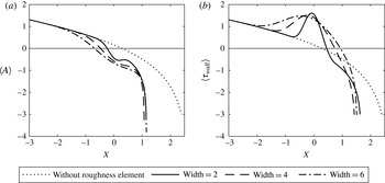
Figure 11. Impact of the dynamic roughness width on the displacement function (a) and skin friction (b), with $\unicode[STIX]{x1D714}=1$ and the roughness midpoint fixed at $X_{M}=0$ . The widths 2 (solid), 4 (dashed) and 6 (dot–dashed) were looked at, with the no-roughness solution given by the dotted line.

The effect of height and frequency of the roughness element seems heavily interlinked: at low amplitudes, there is little difference in the position of zero skin friction at different frequencies, with changes only becoming clear as $a$ is increased. Similarly, for low $\unicode[STIX]{x1D714}$ , there can be little change in the zero skin friction position for a wide range of amplitudes. Overall, figure 12 (produced for $X_{M}=0$ and width equal to 4) shows that above a certain amplitude, there is an inverse relationship between $\unicode[STIX]{x1D714}$ and $a$ : to maintain a given shift in the position of vanishing skin friction, an increase in amplitude has to be compensated by a decrease in frequency and an increase in frequency has to be matched by a decrease in amplitude. We note also that a downstream shift is always seen and that high oscillation frequencies have less of a beneficial impact.

Figure 12. Impact of the frequency ( $\unicode[STIX]{x1D714}$ ) and amplitude ( $a$ ) of a single, positive dynamic roughness placed between $-2$ and 2 on the position of vanishing skin friction, compared to when the roughness is not present. The amplitude was varied from $a=0$ to $a=2.5$ and the frequency from $\unicode[STIX]{x1D714}=0.1$ to $\unicode[STIX]{x1D714}=3.1$ , both in steps of 0.1. The positive numbers seen throughout indicate a downstream shift of the local separation point.

This of course prompts the question as to whether a static or dynamic roughness is better with regard to shifting the zero skin friction position in the mean. The answer is dependent on the choice of roughness parameters: for the selection $X_{L}=-1$ , $X_{R}=3$ , $a=1$ , $\unicode[STIX]{x1D714}=1$ (figure 13), the dynamic roughness is superior, although we note that the singular point is advanced. Comparing the graphs of the time-averaged displacement function, the dynamic roughness introduces a greater favourable pressure gradient into the flow over its front face; the increased shift in the point where $\unicode[STIX]{x1D70F}_{wall}=0$ is due to the addition of two times the roughness shape function to $A$ , rather than just one.

Figure 13. Comparison in the displacement function (a) and skin friction (b) for a dynamic (solid line) and static (dashed line) roughness, placed between $-1$ and 3 and of height 1. For the dynamic roughness, the frequency of oscillation was $\unicode[STIX]{x1D714}=1$ . The solution in the absence of a roughness element is given by the dotted line.

5 Breakaway separation

The downstream singularity that follows the position of zero skin friction throughout is linked to the occurrence of the full nonlinear separation of the boundary layer from the hump surface. In SD, this singularity is removed and the flow development described by considering a region of order $h^{-2}$ length about the singular point (region D of figure 1). Here, we are interested in the possibility of static or dynamic roughness elements moving the singularity downstream, thereby delaying the separation of the boundary layer from the hump surface. Physically, we aim to introduce a large favourable pressure gradient to the flow, expecting that this would serve to prolong the streamwise extent for which the flow is attached. Mathematically speaking, we equate this to a downstream shift of the singular point, $X=X_{s}$ , which can be defined numerically as occurring at the mesh point $n$ where $|A_{n+1}-A_{n}|$ is greater than some moderately large number, taken to be 5.

To this end, we place a roughness element, whose shape is again given by the polynomial form of equation (4.7), with midpoint after the position of the no-roughness singularity, but with left endpoint upstream of it. In the graphs that follow, $X_{M}=6$ and $X_{L}=0$ . The maximum roughness height is chosen to be larger than those considered previously ( $a=5,10,15$ ), but we recall that the roughness is still small (of $O(h^{-5/4})$ ) compared to the amplitude of the hump ( $O(h)$ ) and the inner Goldstein layer in the roughness region ( $O(h^{-7/8})$ ). We hope then that the considerable favourable pressure gradient introduced over the front face of the roughness delays the breakaway separation of the boundary layer.

We see that for a static roughness element this is indeed the case (figure 14), with the singular position delayed for all roughness heights shown. We note, however, that for $a=5$ (solid line), the singularity still occurs on the front side of the roughness element, with it being shifted to the rear side of the roughness element ( $X_{s}>6$ ) only once the roughness height (and hence gradient) is sufficiently large. Comparing the graphs for $a=10$ and $a=15$ , and recalling the pressure–displacement relation $P_{1}=F_{s}A$ (2.29), we see firstly that the larger height gives rise to a more favourable pressure gradient over the front half of the roughness, as would be expected; and, secondly, that there is a slight pressure recovery over the rear face of the roughness ( $a=10$ ) before the singularity is encountered, again as would be expected. The eventual singular point is similar for both $a=10$ and $a=15$ and we suggest that this may be due to the adverse pressure gradient encountered on the lee side of the roughness being greater for increasing height: the effect of an increased acceleration of the flow over the first half of the roughness element being attenuated somewhat by the larger adverse pressure gradient encountered over the second half. In fact, at greater roughness amplitudes, the singular point on the lee side of the roughness element starts moving upstream. For the roughness configuration shown here, we note also the existence of a small region of negative skin friction for the amplitudes $a=10$ and $a=15$ .

Figure 14. Impact of the roughness height on the displacement function (a) and skin friction (b) for a static roughness with left endpoint at $X_{L}=0$ and maximum height at $X_{M}=6$ . The roughness shape was as given in (4.7). The dotted line represents the no-roughness solution.

For dynamic roughness elements, the same numerical method as that described in § 4 was used to obtain the solution for the skin friction, although many more Fourier modes ( $M$ ) needed to be incorporated into the sum (4.3) to ensure the correct position of the singularity. In condition (4.4), $\unicode[STIX]{x1D70F}_{s}=-5$ , with the skin friction decreasing rapidly after this; and the tolerance was typically less than $O(10^{-10})$ . The increased value of $M$ required meant that the step size was increased to $\unicode[STIX]{x1D6E5}=0.005$ to speed up the computation.

Figure 15. As in figure 14, but for a dynamic roughness oscillated with frequency $\unicode[STIX]{x1D714}=0.5$ .

Figure 16. As in figure 14, but for a dynamic roughness oscillated with frequency $\unicode[STIX]{x1D714}=1$ .

Figures 15–17 show that dynamic roughness elements placed with midpoint downstream of the no-roughness singular point but with left endpoint upstream of it are also able to shift the position of the singularity to the right and thus delay the breakaway of the boundary layer from the surface, although not to the same extent as static elements. In particular, the singular point remains on the front face of the roughness element at all heights and oscillation frequencies studied. As per static elements, a greater downstream movement is seen for increasing height; and higher frequencies also have a more beneficial effect. This is to be compared with the conclusions of § 4, where an increase in frequency resulted in a diminished downstream shift of the local separation point. For these larger dynamic roughness elements, centred downstream of the no-roughness singular point, we obtain qualitative agreement with the findings of Huebsch et al. (Reference Huebsch, Gall, Hamburg and Rothmayer2012), who concluded that an increase in frequency allowed one to decrease the roughness height while still maintaining effective flow control. We note that as $\unicode[STIX]{x1D714}\rightarrow 0$ , we do not approach the static solution and instead the singularity moves towards its original, no-roughness position. This is due to the influence of the higher Fourier modes, not present in the static solution and we believe that, physically, this is due to the roughness element dropping flush with the hump surface before returning to its maximum extension over one cycle of oscillation.

Figure 17. As in figure 14, but for a dynamic roughness oscillated with frequency $\unicode[STIX]{x1D714}=1.5$ .