Design margins

In industrial design, design parameters are rarely set to the exact theoretically required values; rather, they often have a margin that might be chosen deliberately or as a consequence of other design decisions. Experienced engineers include such margins in a product design process to serve several purposes. At the outset of the design process of any complex system, requirements, constraints, and capabilities are often uncertain. These uncertainties result from engineering change or for accommodating product flexibility and future growth (Eckert and Isaksson, Reference Eckert and Isaksson2017). To cover these uncertainties, designers tend to add margins to the design parameter values based on their past experience to cover realistic requirements and later firm up these values with analysis and testing (Eckert et al., Reference Eckert, Isaksson and Earl2019).

The design of large projects involves collaboration from multiple teams working in parallel to tight schedules and budget constraints. The design process typically involves multiple pre-planned iterative revisions to gather inputs and integrate results from the parallel teams (Wynn and Eckert, Reference Wynn and Eckert2017). During these iteration rounds, key requirements and key parameters can change significantly, forcing other teams to accommodate these changes, and hence, a margin is added to protect against design uncertainties (Eckert and Isaksson, Reference Eckert and Isaksson2017). In collaborative complex system designs, these margins are estimated in negotiation between design teams (Austin-Breneman et al., Reference Austin-Breneman, Yu and Yang2015). These margins provide a certain level of isolation between design parameter choices so that a minor change to one design parameter does not force an immediate review of every other possible independent design parameters. Examples of such design parameters with lower and upper margins are: power, pressure, level, temperature, pH, composition, and flow rate.

Design margins also play a critical role in safely managing engineering change and iteration. Designers and engineers define upper and/or lower margins to form an envelope called the “Safe Design Envelope (SDE)” for the chosen equipment (Eckert et al., Reference Eckert, Isaksson and Earl2019; Stauffer and Chastain-Knight, Reference Stauffer and Chastain-Knight2019). These envelopes establish Safe upper and lower Operating Limits (SOLs) for critical operating parameters, beyond which there is a risk of catastrophic equipment failure. SOLs aim is to prevent process safety incidents and must be identified and documented for effective management of safety (Dowell, Reference Dowell2001; Richardson, Reference Richardson2012; Forest, Reference Forest2018).

The Center for Chemical Process Safety (Guidelines for safe automation of chemical processes 1993) advise multiple layers of protection are used to protect people, property, and the environment from the hazards of chemical processing. This leads to a formal design approach entitled Layers Of Protection Analysis (LOPA; Willey, Reference Willey2014) that ensures safety systems are multiply redundant. The LOPA design philosophy requires that critical parameters have a margin defined during design, referred to as normal operating limits, safe operating limits, instrumentation limits, and equipment containment limits (Stauffer and Chastain-Knight, Reference Stauffer and Chastain-Knight2019).

Buchan and Bolton pointed out that system reliability and safety depend on an inherently safe design (ISD; Pandian et al., Reference Pandian, Hassim, Ng and Hurme2015), and this requires that a high degree of rigor is applied to design and fault analysis (Buchan and Bolton, Reference Buchan and Bolton2009). Active systems rely on their ability to detect a system moving out of its safe envelope, whereas passive systems provide more safety and reliability by applying inherently safer design at the earliest stages of the project design process. The passive features generally involve less components that are easier to characterize and whose design parameters form a safe operating envelope. One challenge is to ensure that these design limits are fully understood and complied with during the system's lifecycle. Design margins are not only applied in chemical processing but also in many other areas such as power generation (Sutherland, Reference Sutherland2011), jet engine design (Eckert et al., Reference Eckert, Isaksson and Earl2019), civil engineering (Buchan and Bolton, Reference Buchan and Bolton2009), and nuclear power plants (Modarres, Reference Modarres2009). Setting insufficient margins for critical parameters can result in catastrophic accidents such as the collapse of [in]famous Tacoma Narrows Bridge (Buchan and Bolton, Reference Buchan and Bolton2009), whereas overestimating margins results in overdesign and higher build costs. Eckert also argues that awareness of margins during the design process can lead to more efficient management of change processes (Eckert and Isaksson, Reference Eckert and Isaksson2017).

Multiple factors contribute to these margins. The operation of process plants or their components results in hidden variables not captured in the design dataset. For instance:

• • A fluid may have frictional energy loss as it moves along a pipeline changing its pressure and/or temperature properties in accordance with some (hidden) distance variable.

• • Pumping of fluids may change its pressure property in accordance with some (hidden) pump capacity variable.

• • The fuel efficiency of engines may vary in accordance with some (hidden) cylinder diameter variables.

General regression neural network

Industrial design outcomes are influenced by a combination of design parameters of single or multiple dimensions. Determining the correlation between dependent and independent variables for a system or process can be difficult. Traditional approaches have limitations when modeling complex nonlinear systems. Artificial Neural Networks (ANNs) have been found to solve such tasks better in many practical applications (Aglodiya, Reference Aglodiya2017).

The General Regression Neural Network (GRNN) is a term coined by Donald F. Specht (Specht, Reference Specht1991), for a family of ANNs derived from the statistical technique of Nadaraya–Watson kernel regression (Nadaraya, Reference Nadaraya1964; Watson, Reference Watson1964). GRNNs are single-pass associative memory feed-forward type ANNs and are generally used for function approximation. GRNNs have been widely used for approximation, fitting, prediction, and regression problems in the industry for fault detection and diagnosis (He and He, Reference He and He2011; Baqqar et al., Reference Baqqar, Wang, Ahmed, Gu, Lu and Ball2012; Li et al., Reference Li, Zhao, Ni and Zhang2018; Niu et al., Reference Niu, Tong, Cao, Zhang and Liu2019), batch processing and system identification (Kulkarni et al., Reference Kulkarni, Chaudhary, Nandi, Tambe and Kulkarni2004; Ou and Hong, Reference Ou and Hong2014; Al-Mahasneh et al., Reference Al-Mahasneh, Anavatti and Garratt2018), building systems monitoring (Kim and Katipamula, Reference Kim and Katipamula2018; Mohandes et al., Reference Mohandes, Zhang and Mahdiyar2019), and in other areas of engineering (May et al., Reference May, Maier, Dandy and Nixon2004; Cigizoglu and Alp, Reference Cigizoglu and Alp2006; Pal and Deswal, Reference Pal and Deswal2008; Kumar and Malik, Reference Kumar and Malik2016; Lee et al., Reference Lee, Kim and Jun2018; Jagan et al., Reference Jagan, Samui and Kim2019). The GRNN algorithm is efficient, and it can learn high-dimensional mappings in a single pass and results in acceptable performance even with a tightly constrained training set (Specht, Reference Specht1991). Furthermore, it has only a single tuning parameter to achieve function smoothing, unlike the Back Propagation Neural Network (BPNN) and Support Vector Regression (SVR) that require multiple parameters to be tuned, needing more computational time and training data (Celikoglu and Cigizoglu, Reference Celikoglu and Cigizoglu2007; Zhang et al., Reference Zhang, Wang, Zhu and Zhang2012; Jiang and Chen, Reference Jiang and Chen2016). The estimation of the GRNN smoothing parameter also has the advantage that it is not prone to local minima, unlike other methods such as BPNNs (Pal, Reference Pal2011; Niuet al., Reference Niu, Liang and Hong2017).

Outlier detection

Outlier detection (Hodge and Austin, Reference Hodge and Austin2004; Singh and Cantt, Reference Singh and Cantt2012; Zimek et al., Reference Zimek, Schubert and Kriegel2012; Patil and Chouksey, Reference Patil and Chouksey2016; Ge et al., Reference Ge, Song, Ding and Huang2017; Xu et al., Reference Xu, Liu, Li and Yao2018) has been gaining prominence as an area of machine learning (Ge et al., Reference Ge, Song, Ding and Huang2017; Xu et al., Reference Xu, Liu, Li and Yao2018). In other published work, supervised, semi-supervised, and unsupervised methods have all been used for outlier detection (Hodge and Austin, Reference Hodge and Austin2004; Singh and Cantt, Reference Singh and Cantt2012; Xu et al., Reference Xu, Liu, Li and Yao2018). Among the unsupervised methods, two commonly used approaches to detect outliers are: statistical models to estimate a probability density function (p.d.f) using methods such as Parzen window (Parzen, Reference Parzen1962; Mussa et al., Reference Mussa, Mitchell and Afzal2015; Wang et al., Reference Wang, Bah and Hammad2019); and ANNs that establish the relationship between variables as a regression model such as the GRNN (Specht, Reference Specht1991; Kartal et al., Reference Kartal, Oral and Ozyildirim2018; Wang et al., Reference Wang, Bah and Hammad2019). Unsupervised methods can learn directly from industrial design datasets, offering clear economic benefits, and use these models to validate data by detecting outliers. Outlier detection has become a field of interest for many practitioners of fault detection and diagnosis (Zimek et al., Reference Zimek, Schubert and Kriegel2012; Xu et al., Reference Xu, Liu, Li and Yao2018; Blazquez-Garcia et al., Reference Blazquez-Garcia, Conde, Mori and Lozano2020). This paper investigates two different methods for outlier detection using a modified GRNN and the long-established Parzen method.

A new method for outlier detection

Most previous research work uses the GRNN algorithms to derive a single regression model either to be used as a prediction tool or to estimate the accuracy of data. An extension from this approach is presented in this paper using a novel method called the Margin-Based GRNN (MB-GRNN). It uses a modified GRNN for the estimation of upper and lower regression boundaries (also called margin boundaries) by deriving three interlinked regression models from the same dataset. These margin boundaries, derived directly from data, can be used as a classifier to detect outliers or to determine the maximum and minimum values of dependent variables for any given design parameters. To obtain the best estimate of these margin ranges, the model must achieve the best possible generalization of the data and stretch out the extremal margin boundaries to the appropriate extent. To achieve the best generalization, the leave-one-out cross-validation (LOOCV) method (Specht, Reference Specht1991) is applied using a more systematic approach to derive features from data involving clustering, k-nearest neighbor, and individual covariance. The motivation for adding stretching factors to a GRNN comes from papers that have weighted the terms of a GRNN to achieve computational gains (Lee and Zaknich, Reference Lee and Zaknich2015) and the weighted version of Nadaraya–Watson estimator to determine a conditional mean (Cai, Reference Cai2001). The MB-GRNN method builds on these approaches by adding stretch factors as a “second kernel factor” to the GRNN to iteratively inflate the extremal margin boundaries. The GRNN has not been previously used in this way to determine the design margins by stretching the regression surfaces to extremes of the range of typical values, so that any atypical combinations located outside of the regression surfaces can be identified as potential outliers. These outliers may be indicative of a design fault or data entry error and warrant further investigation by the design engineers.

The investigation uses both single and multidimensional sample domains that display margin characteristics and use an unsupervised approach to learn from data without the need for specific knowledge of the function of components. Two methods to detect outliers are assessed here, contrasting their performance on this class of problems. The first probabilistic method applied uses a clustering (Berkhin, Reference Berkhin2002) algorithm to find a set of neighboring vectors and uses Parzen window (Parzen, Reference Parzen1962) to estimate p.d.fs comprised of standard Gaussian kernels with optimized parameters. The second method is the MB-GRNN regression algorithm, developed by applying stretch factors as a second kernel term to the GRNN to detect outliers of data. In each case, optimum generalization is achieved by applying a “smoothing parameter” using the LOOCV method.

Parzen window estimator

Parzen window density estimation (Parzen, Reference Parzen1962) is a nonparametric estimation method, which can estimate the joint probability density function p(x, y) of multivariate data evaluated at ${\boldsymbol x}\in {\cal R}^d$ and $y\in {\cal R}^1$, based on a set of samples S _train, comprised of N vectors {c_i}, where each ${\boldsymbol c}_i\in {\cal R}^{d + 1}$ and c_i = (x_i, y _i). The p.d.f is an estimation of the average density in proximity to (x, y). The standard equation for a Parzen window estimator is defined as:

(1)$$p( {{\boldsymbol x}, \;y} ) = \displaystyle{1 \over N}\sum\limits_{i = 1}^N {\phi ( {( {{\boldsymbol x}, \;y} ) \vert {\boldsymbol c}_{i, }{\rm \Sigma }_i} ) },$$

where ϕ((x, y)|c_i,Σ_i) is a kernel function of x parameterized by a central location c_i and covariance matrix Σ_i. A set of training examples S _train provides the central locations for the kernel functions in Eq. (1).

The model is continuous over the domain $\;{\cal R}^{d + 1}$ for the given training sample S _train and a kernel function ϕ(x, y). The implementation uses a Gaussian kernel function with x treated as a row vector:

(2)$$\phi ( {( {{\boldsymbol x}, \;y} ) \vert {\boldsymbol c}_{i, }{\rm \Sigma }_i} ) = \left[{\displaystyle{1 \over {\sqrt {{( {2\pi } ) }^d\vert {{\rm \Sigma }_i} \vert } }}} \right]\exp \left({\displaystyle{{-D^2( {( {{\boldsymbol x}, \;y} ) , \;{\boldsymbol c}_i\vert {\rm \Sigma }_i} ) } \over 2}} \right).$$

And the Mahalanobis distance D (De Maesschalck et al., Reference De Maesschalck, Jouan-Rimbaud and Massart2000) is defined as:

(3)$${\rm D}( {{\boldsymbol A}, \;{\boldsymbol B}\vert {\rm \Sigma }} ) = \sqrt {( {{\boldsymbol A}-{\bf B}} ) {\rm \Sigma }^{{-}1}{( {{\boldsymbol A}-{\bf B}} ) }^T}. $$

The distance D _i((x, y),c_i|Σ_i) is measured between a vector (x, y) and c_i, the central location of a kernel, weighted by Σ_i. When x is multidimensional, the Mahalanobis metric provides elliptical equidistance boundaries with covariance Σ determining the major and minor axes. D can be used to determine the spread of points forming a cluster from its central point if the covariance is used as the normalizing measure (De Maesschalck et al., Reference De Maesschalck, Jouan-Rimbaud and Massart2000).

Covariance determination

Covariance, in the statistical sense, is a measure of the correlation between two variables (Dempster, Reference Dempster1972). In a multidimensional domain, the covariance matrix ${\rm \Sigma }_i\in {\cal R}^{dXd}$, captures the correlation between each pair of the dimensions.

The Parzen estimator uses a covariance matrix Σ_i that just considers the set of neighbors S _i in proximity to each c_i and the method applied was to calculate the covariance matrix for the set of n nearest neighbors (Cover and Hart, Reference Cover and Hart1967). The covariance matrix is calculated for vector c _ij using:

(4)$${\rm \Sigma }_{ijk} = \displaystyle{1 \over n}\sum\limits_{\,p\in S_i} {( {{\boldsymbol c}_{\,pj}-\mu_j} ) ( {{\boldsymbol c}_{\,pk}-\mu_k} ) },$$

where $\mu _k = 1/n\;\sum\nolimits_{p\in S_{i},} {{\boldsymbol c}_{pk}}$ is the mean and n is the number of elements in the neighborhood set S _i and (j, k) are each in the range [1,d] and select an element within the Σ_i matrix. The additional variable p is an index used to select the subset of c_i values that are members of the neighbors set S _i.

Equation (4) takes into account the local variation of density in a region around c _i. The choice of n specific to each training dataset is critical in determining the Mahalanobis distance metric, as covariance acts to scale the Mahalanobis distance. The covariance needs to be further scaled to provide a smooth generalization between neighbors, and this must be done as a separate optimization exercise for each training dataset using a scaling factor. The neighborhood set S _i is determined for each n chosen from a range of values and the optimum scaling factor is determined for each n as shown in Figure 3.

Scaling factor

The covariance calculation described in Eq. (4) represents the distribution of n neighboring points around a mean μ. However, it alone does not ensure smooth interpolation between neighbors. The covariance matrix can be further optimized by determining a scalar multiplier s (referred to as the scaling factor). The scaling factor is determined using the LOOCV method that involves omitting one sample at a time and constructing the network based on the remaining samples. This network is then used to predict the probability value of the omitted sample, and this is averaged (Xu et al., Reference Xu, Zhang, Zhu and He2013) by iterating over the entire set. The purpose of this method is to find the solution that maximizes the average probability of samples using the Parzen estimate as shown in Figure 2 (or to develop a regression model for a known variable by minimizing mean squared errors using the GRNN model as shown in Fig. 3). The scalar factor s is then multiplied by the individual covariance Σ_i to give the optimum model fit for both Parzen and GRNN models.

The scaling factor is obtained by multiplying the covariance by a range of scaling values and iteratively repeating the above process to find the best factor s that maximizes the average probability (or minimizes the mean squared error) of samples for the entire distribution. The optimization process is shown in Figure 1 and the section “Smoothing parameter determination for Parzen and GRNN methods (Refer Step 3 in Fig. 1)”.

Fig. 1. Schematic diagram of Parzen and MB-GRNN application for outlier detection and prediction (for variable notations, refer Table A.1).

To avoid making an arbitrary choice regarding the number of neighbors n that influence the covariance, the scaling factor s can be determined for a range of n and the optimum solutions chosen as shown in Figures 2 and 3, to generate the model. It was found experimentally that, where vectors have very nonuniform distributions, choosing the n nearest neighbors may not give the desired width for the covariance and to avoid this, a vector quantization algorithm attributed to Linde, Buzo, and Gray (LBG; Linde et al., Reference Linde, Buzo and Gray1980) was applied as shown in the section “Pseudocode for data preprocessing and clustering to remove near duplicates (Refer Steps 1 and 2 in Fig. 1)”. This was used as a preprocessing step to find the optimum number of clusters z and these clusters were used in place of the neighboring samples n. This method aims to eliminate duplicates and minimize the influence of closely spread points (near duplicates) when determining covariance.

Fig. 2. Parzen: selection of scaling factor (s) for (n) neighbors.

Fig. 3. GRNN: selection of scaling factor (s) for (n) neighbors.

The LOOCV method can be applied again to determine the optimum number of neighbors n for a given constant s, resulting in minimizing the mean squared error (MSE) or maximizing the average probability (MAP) for the given sample set are shown in Figures 2 and 3, respectively.

GRNN model

The value of a dependent variable y is predicted by a GRNN using the joint p.d.f estimated from known training data. The resulting regression equation can be implemented in a parallel neural network structure to predict the expected value of y for a given x, using (Specht, Reference Specht1991):

(5)$$E[ {y \,\vert \, {\boldsymbol x}} ] = \displaystyle{{\mathop \int \nolimits_{-\infty }^{ + \infty } y\phi ( {{\boldsymbol x}, \;y} ) dy} \over {\mathop \int \nolimits_{-\infty }^{ + \infty } \phi ( {{\boldsymbol x}, \;y} ) dy}},$$

where ϕ(x, y) is the joint continuous p.d.f. In practice, the joint continuous p.d.f can be empirically estimated using Parzen window estimation from a finite set of training examples. As this approach is nonparametric, the model parameters are derived directly from the training set using kernel functions. Rectangular and Gaussian kernel functions are commonly used for multidimensional datasets (Cristianini and Shawe-Taylor, Reference Cristianini and Shawe-Taylor2000). The GRNN determines the most probable value of y for a given value of x as a prediction, whereas Parzen determines a joint probability p(x, y).

Specht redefined the radial basis function model as an interpolator to give y = f(x) that is related to Parzen window. He also observed that the GRNN could learn from training datasets of the form, S _train ≡ {(c_i, y _i)} for 1 ≤ i ≤ N, a set of N training examples that are representative of the underlying probability distribution. Unlike in the case of the Parzen window (Section “Parzen window estimator”), the GRNN's c_i is a d dimensional variable ${\boldsymbol c}_i\in {\cal R}^d$ and c_i = x_i. The y _i values are used to weight the kernels on the numerator but not the denominator of Eq. (6). As discussed in the section “Scaling factor”, the scaling factor s is applied to optimize the width of covariance matrices, to result in correct scaling for y _i “heights”. The functional form of the equation thus becomes:

(6)$$f( {{\boldsymbol x}\;\vert \;{\boldsymbol c}_i, \;{\rm \Sigma }_i, \;s} ) = \displaystyle{{\sum\nolimits_{i = 1}^N {y_i\phi ( {{\boldsymbol x}\;\vert \;{\boldsymbol c}_i, \;{\rm s}{\rm \Sigma }_i} ) } } \over {\sum\nolimits_{i = 1}^N {\phi ( {{\boldsymbol x}\;\vert \;{\boldsymbol c}_i, \;{\rm s}{\rm \Sigma }_i} ) } }}.$$

Proposed MB-GRNN model

Apart from the use of the GRNN as a predictor to define a control function, this paper presents a new Margin-Based GRNN (MB-GRNN) approach for outlier detection by defining upper and lower margin boundaries for a given dataset. This is achieved by adapting the GRNN algorithm, by applying stretch factors as a second kernel weighting factor. As stated in the section “A new method for outlier detection”, the idea of weighting each one of the terms as shown in Eq. (7) with an additional weighting w _i has previously been used by other researchers (Cai, Reference Cai2001; Lee and Zaknich, Reference Lee and Zaknich2015). The MB-GRNN takes the form:

(7)$$f( {{\boldsymbol x}{\rm \;}\vert {\rm \;}{\boldsymbol c}_i, \;{\rm \Sigma }_i, \;s, \;w_i} ) = \displaystyle{{\sum\nolimits_{i = 1}^N {y_iw_i\phi ( {{\boldsymbol x}{\rm \;}\vert {\rm \;}{\boldsymbol c}_i, \;{\rm s}{\rm \Sigma }_i} ) } } \over {\sum\nolimits_{i = 1}^N {w_i\phi ( {{\boldsymbol x}{\rm \;}\vert {\rm \;}{\boldsymbol c}_i, \;{\rm s}{\rm \Sigma }_i} ) } }}.$$

The computational complexity to evaluate f(x) in Eq. (7) uses time O(Nd ²) and the calculation is well suited to vector processing methods. By choosing the correct set of stretch factors w _i, the GRNN can be made to follow the extremal upper or lower margin boundaries of a data cloud. The choice of stretch factors pushes the margin boundaries outward based on the characteristics of data. The resulting boundaries not only classify the data outliers but also can be used as a range predictor of y for any given x as shown in Figure 6. An approach for choosing the stretch factors w _i is described in the section “New margin-based GRNN (MB-GRNN) model using stretch factors”.

Experimental data and its characteristics

Analysis of design datasets has highlighted the widespread use of design margins. When viewed as a regression problem, and for design parameters x (independent variables), when a regression model g is learned from data such that y = g(x), it was found that the resulting scalar variable y (dependent variable) inhabits a range [y _min, y _max], often with fairly uniform density, such that y _min ≤ g(x) ≤ y _max. However, unlike the margin applied to support vector regression problems, the range m is not of fixed width but depends on x such that y _max = y _min + m(x). These ranges can be observed directly from experimental datasets, such as those in Figures 7 and 9. This creates the possibility of adopting a classification approach to detect outliers outside these typical design margins y _min or y _max.

Three publicly available engineering multivariate design datasets were chosen for the experiment that displays the characteristics of margins. The first dataset used for experimental testing is called the “Auto MPG Data Set” and is from the UCI machine learning repository (Repository, 1993). It describes automobile fuel consumption for a set of multivalued discrete and continuous design parameters. The second set is an “Energy Efficiency Data Set” also from the UCI machine learning repository (Repository, 2012) that documents the heating and cooling loads of buildings based on their design parameters. The final dataset is a “Concrete Design Data Set” from the same source (Repository, 2007), describing the compressive strength of concrete based on the composition of ingredients. These datasets were selected as they relate directly to the design parameters of engineered artifacts and also have specific characteristics with multiple values of the dependent variables y for each value of the independent variable x (e.g., see Figs. 7 and 9). Use of these experimental datasets from multiple domains also suggests the versatility of the approach for other datasets having similar characteristics.

Data description

For the Parzen window approach, data were processed in the format (x, y) for N samples where each vector x = (x ₁, x ₂, x ₃, x ₄,…, x _d), and for the MB-GRNN models, x was used as the independent variable and scalar y as the dependent variable. Parameters used from the experimental datasets are listed in Table 1.

Table 1. Experimental dataset parameters

The Python language and the Spyder IDE were used to process data, develop algorithms, and present results in graphical and tabulated formats. The implemented algorithms deal with both single and multiple dimensional data, and these datasets are used to explain the experimental results and analysis.

Schematic diagram of the method proposed

The schematic diagram, as shown in Figure 1, describes the overview of the processing steps applied for outlier detection and margin prediction.

Data preprocessing and clustering (Steps 1 and 2 in Fig. 1)

Section “Data description” describes the selection of variables for each data and array format. Each datum was first transformed onto a logarithmic scale to lower the skewness of its data distribution, improving the interpretation of data. The transformed data were normalized by linearly mapping each data to the unit interval [0,1] to improve training efficiency and to minimize the risk of certain variables being given more significance, especially when they represent different orders of magnitude (Patton, Reference Patton1995).

The LBG vector quantization algorithm was used to segregate input data into an optimum number of clusters z to eliminate duplicates and minimize the influence of near duplicates. The optimum number of clusters z and the cluster mean values μ are further used to determine optimum covariance. The pseudocode for the LBG algorithm is explained in the section “Pseudocode for data preprocessing and clustering to remove near duplicates (Refer Steps 1 and 2 in Fig. 1)”.

Determination of scaling factor and optimum covariance (Step 3 in Fig. 1)

The covariance matrix Σ_i is calculated by choosing a suitable set of neighbors with n members in the range 1 ≤ n ≤ z, and a multiplicative factor called the scaling factor s that provide appropriate smoothing for Σ_i. The scaling factor s is determined using the LOOCV method, as described in the section “Smoothing parameter determination for Parzen and GRNN methods (Refer Step 3 in Fig. 1)”. Figure 2 shows the graph of average probability versus scaling factors in the range [0.1,3] for neighbors n in the range [4,19]. The optimum scaling factor s _opt = 0.53939 that maximizes the global average probability was obtainedFootnote ¹ when n = 4 and is used to determine optimum covariance (s _optΣ_i) when calculating the Parzen p.d.f.

Figure 3 shows the graph of GRNN mean squared error versus scaling factors in the range [0.1,3] for neighbors n in the range [3,19]. The optimum scaling factor s _opt = 0.25757 that maximizes the global average probability was obtainedFootnote ¹ when n = 16 and is used to determine optimum covariance (s _optΣ_i) when calculating the smoothing parameter. The computational complexity to find the optimal value of s requires time O(N ²d ²) and memory O(Nd ²) and is largely determined by the calculation of the leave-one-out metrics. The method is well suited to a range of established bounded optimization techniques since the error surfaces are scalar, smooth, and typically have a global minimum/maximum. Experiments were conducted using various bounded, and root-finding optimization functions for the three datasets presented in this paper. The results suggest significant savings in computational time to reach the convergence. A novel derivative function was used for root-finding functions, and these methods and experimental results will be presented in a future paper.

Parzen window p.d.f estimate

The implementation uses a Gaussian window function to estimate the density of samples using the optimized covariance obtained in Eq. (4). Figure 1 shows the steps involved, and the overall implementation uses Eqs (1)–(3).

New MB-GRNN model using stretch factors

The MB-GRNN implementation involves determining three inter-related GRNN models: for the middle, upper, and lower boundaries. These boundaries provide a way of ordering outliers to measure the distances beyond the typical limits using an error margin Error >0 as outlined in S23a and S23b of Table A.3. Firstly, a conventional GRNN model (providing the middle boundary) is found to segregate the data into the upper and lower subsets, and subsequently, the upper and lower boundaries are determined using two stretched GRNNs.

Determination of the upper and lower GRNN boundaries

For each of the two segregated upper and lower datasets, the optimum number of clusters z, scaling factor s _opt, and optimum covariance matrix s _optΣ_i were estimated. A set of four stretch factor thresholds were chosen $\hat{w} = ( {0.03, \;\;0.1, \;\;0.3, \;\;0.5} )$ for the experiment. These specific values were not found to be critical for success as they appear both in the numerator and denominator of the GRNN, and so they self-normalize. However, it is important that the values must span a wide range of at least two orders of magnitude to ensure that some points have more prominent weightings than others. The MB-GRNN was used to generate upper (or lower) GRNN models using Eq. (7), by applying the weight thresholds iteratively for datasets that lie within the upper and lower boundaries. This iterative process pushes out the upper (or lower) boundaries by ensuring that points closer to the upper and lower boundaries have a higher weighting than the interior points. The process shown in Table A.3 shows the greedy algorithm that was developed for determining the stretched upper and lower GRNN margin boundaries.

For this algorithm, a stretch factor threshold with M = 4 iterations was chosen as a trade-off between computational efficiency and performance. However, a convergence criterion could be applied for a range of stretch factor thresholds until no new data points get shifted from $\delta _i^u > 0$ to $\delta _i^u \le 0$ in any subsequent iteration for upper boundary and vice versa for lower boundary. The computational time of the stretch algorithm grows approximately linearly with M resulting in O(MN + N ²d ²) since the optimal scaling factor s need to be re-estimated once each for the upper and lower datasets, whereas the memory requirement is O(Nd ²). Figure 4 shows the outcome of an experiment utilizing artificial data and using a known function 0.1sin 9x + 0.75 (only the upper GRNN curves are shown for clarity). The orange curve shows the middle GRNN, the blue curve shows the surfaces for each stretch step iteration, the green curve shows the stretch boundary after eight stretch steps, and the red curve shows the artificially generated upper surface for the known function. Eight stretch factor thresholds were used in a uniform logarithmic scale between 10⁻² and 1. Figure 5 shows the progression of the stretch steps and MSE calculated for each stretch step against the known function. The experimental results suggest that the optimum performance is obtained after the first four stretch steps, after which the difference in MSE is nominal.

Fig. 4. Progression of stretch algorithm.

Fig. 5. Stretch steps and MSE.

Once the GRNN upper and lower boundaries are determined using the stretch iterations, either points that lie outside of the extremal boundaries can be nominated as outliers as explained in the section “Experimental results and analysis”, or a reliability threshold can be applied using a distance metric to identify outliers and near outliers as explained under the section “Experimental results and outlier detection”.

AutoMPG dataset

Firstly, results and analysis for a univariate dataset, consisting of 199 examples, are explained to introduce the upper and lower GRNN margin boundaries derived using an MB-GRNN. This method is compared with the Parzen probabilistic approach. Later, results and analysis will focus on multivariate datasets.

The similarities and differences between the MB-GRNN and Parzen methods are indicated using color codes and markers. The colors and markers used in figures and legends have been kept consistent and are explained immediately below.

Each example was ranked in order of its Parzen probability with low probability, suggesting that a point might be an outlier. Data points that are outside the upper or lower GRNN boundaries as estimated by the MB-GRNN are treated as outliers with Error >0. Outliers estimated by the MB-GRNN are compared with the 25 lowest Parzen probabilities shown in Figures 6, 7, 9 and 10.

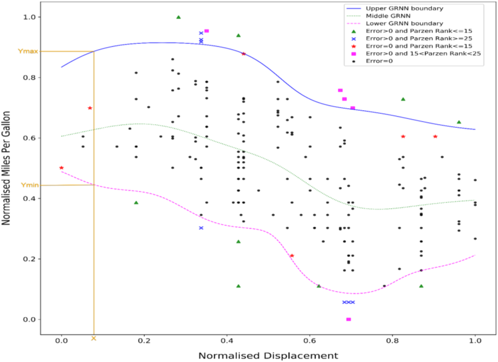
Fig. 6. AutoMPG univariate outlier detection: MB-GRNN and Parzen plots.

Fig. 7. AutoMPG multivariate outlier detection: MB-GRNN and Parzen.

Fig. 8. Parallel coordinates plot of outliers for data points in Table 2 (black is hidden from the plot so as not to overwhelm the plot).

Fig. 9. Energy efficiency multivariate outlier detection: MB-GRNN and Parzen.

Fig. 10. Concrete multivariate outlier detection: MB-GRNN and Parzen.

Table 2. Analysis of results of AutoMPG multivariate dataset with (${x}_1, \;{ x}_2, \;{x}_3, \;{ y}$) variables

The small black dot “.” denotes points that are not detected as outliers by the MB-GRNN (Error = 0 as per S23a and S23b of Table A.3) and have higher Parzen probability ranking ≥25, indicating agreement between the two methods.

The green colored “” data points also show cases with a very high degree of agreement between the two methods since the MB-GRNN identified them as outliers with the cost of error >0, and they also have Parzen least probability ranking ≤15. These denote most likely outlier points.

The magenta colored “” symbol shows the outliers identified by MB-GRNN (Error > 0) and with least Parzen probabilities ranking <15 and ranking >25, nominating them as potential outliers. The thresholdsFootnote ² 15 and 25 were chosen as they correspond to 7.5% and 12.5% of points in the dataset, respectively.

The red color “” data points are cases where the two methods disagree. They were not predicted as outliers by the MB-GRNN (Error = 0) but are within the lowest 15 Parzen probabilities. These data points are in regions with low point densities either at the extremities of the x domain or between higher density regions within the range. Due to MB-GRNN's interpolativeFootnote ³ property, these points are judged by their y values being located between the upper and lower surfaces.

On the other hand, the blue data points “” were identified as legitimate outliers by the MB-GRNN (Error > 0), and where least Parzen probabilities were ranked ≥25. These data points were either above or below the extremal boundaries determined by the MB-GRNN.

The outlier classifications from both the MB-GRNN and Parzen methods for the selected univariate dataset are shown in Figure 6. Each case is color coded to show the degree of agreement or disagreement between the two methods. There is a high degree of correlation between the two methods (the black dots); however, some results contrast due to the different approaches.

The Parzen and MB-GRNN methods use similar optimization techniques to determine the scaling factor and covariance matrix as described previously in the section “Determination of scaling factor and optimum covariance (Step 3 in Fig. 1)”. Unlike the conventional GRNN that only determines the line of best fit, the MB-GRNN can determine the upper and lower boundaries of the dataset to predict a range of legitimate y values for any given x and use these boundaries as the limiting “fence” to identify the possible outliers as shown in Figure 6. Unlike some other regression methods, such as those based on support vectors (Cristianini and Shawe-Taylor, Reference Cristianini and Shawe-Taylor2000), that provide a constant width band of insensitivity, the MB-GRNN determines design margins that reflect the data distribution. These results suggest that the proposed MB-GRNN method can be a useful approach for the industry datasets that have a range of y values for any given x.

Figure 7 compares the result of two different methods for a multivariate dataset (x ₁, x ₂, y). The results suggest that the MB-GRNN and Parzen methods identify different types of outliers. The MB-GRNN predicts outliers that are outside the upper and lower regression surfaces formed using a weighted conditional expectation on the chosen dependent variable y and independent variable x, whereas the Parzen method uses a joint probability for the combination of (x, y). Both methods have merits in identifying outliers as Parzen predicts the least probable data points by estimating lower probabilities, whereas the MB-GRNN predicts outliers based on a chosen dependent variable.

Compared to the univariate dataset, greater discrepancies were observed between the MB-GRNN and Parzen methods for datasets with multivariate independent variables. For the most isolated points, the green color “” and magenta colored “” data points show a high degree of agreement between the two methods. From Figure 7, it can also be observed that the red “” data points are outliers effectively detected by Parzen, and the blue colored “” maximal/minimal data points are outliers best detected by the MB-GRNN. Just like Figure 6, the red “” are at the extremities of the domain, and the blue “” / magenta “” are at the extremities of the range.

Table 2 shows the result of the two different methods applied to a four-dimensional multivariate dataset (x ₁, x ₂, x ₃, y) and Figure 8 shows the parallel coordinates plot of outliers detected by both methods. The data points with MB-GRNN errors (Error > 0) shown in green-dashed, magenta-dashdotted, and blue-solid categories and Parzen outliers not detected by MB-GRNN (Error = 0) are shown in the red-dotted category. These results follow a similar pattern with previous experiments presented above.

The green-dashed, magenta-dashdotted, and blue-solid category data points in Figure 8 indicate the outliers identified by the MB-GRNN, due to a single or a combination of independent variables (x ₁, x ₂, x ₃) having unexpectedly low or high values. The green-dashed and magenta-dashdotted points were also identified as outliers by the Parzen method as one or more variables (x ₁, x ₂, x ₃, y) were extremal in the domain with ranking MB-GRNN Error > 0 and 0 < Parzen Rank <25. For example, the data point with minimum miles per gallon (value 18) was identified as a green-dashed category outlier, and this was due to high values of displacement, horsepower, and weight (values 121, 112, and 2933, respectively), resulting in lower fuel economy. Both Parzen and MB-GRNN methods identified this data point as an outlier, as it is positioned at the extremities of both range and domain. Whereas the maximum miles per gallon (value 46.6) is shown as a blue-solid category outlier due to relatively low values of displacement, horsepower, and weight (values 86, 65, and 2110), resulting in higher fuel economy. This data point was identified as an outlier by the MB-GRNN due to it being located in the extremities of the range. However, Parzen did not find this data point as an outlier as it was not located on the extremities of the domain. The red-dotted category data points were identified as outliers by the Parzen method due to a single or a combination of variables having significantly low or high values in the domain. An example of red-dotted data point is with displacement, horsepower, weight, and MPG values of 72, 69, 1613, and 35, respectively, with displacement and weight having low values in the domain. The results suggest that both Parzen and MB-GRNN can complement each other to detect outliers in the domain and range (for a given value of y), respectively.

Energy efficiency and concrete datasets

Figures 9 and 10 show the upper and lower margin boundaries for the energy efficiency and concrete multivariate design datasets. The algorithm and optimization techniques identical to that of AutoMPG were applied to these datasets. The results are consistent with the AutoMPG dataset presented in Figure 7.

The building energy efficiency data shown in Figure 9 can be seen to be heavily quantized in the domain, having a wide range of y values for a given x. Even with such quantized data, the MB-GRNN was able to predict margin boundaries and pick the blue colored “” points as outliers to identify values that are away from the distribution. The red “” data points identified as outliers by Parzen being extremal points in the domain.

For the concrete dataset shown in Figure 10, the upper and lower boundaries are more complex. Despite this, the solution still only finds a small fraction (18%) of data points as outliers by combined Parzen and MB-GRNN methods.

Adaptation for incremental learning

Any online implementation of the algorithm described should deal efficiently with the inclusion of a new data point (x,y) into S _train. The GRNN is a nonparametric model, so parameter re-estimation is not required with the advent of additional data points. However, the computational complexity of evaluating the model grows linearly with N, so any software implementation might need to limit N by, for instance, avoiding near duplicates to existing data or aging data measurements so that outdated measurements are excluded from consideration.

Although the GRNN itself is nonparametric, there are three parameters described elsewhere in this method. The first is derived from nearest neighborhood distance sets S _i, so the advent of a new data point would only affect one n-neighbor set and necessitate recalculation of one covariance matrix Σ_i at computational time complexity O(Nd ²).

The second parameter is the scalar stretch scaling s. The advent of one new data point would have little impact on the margin estimates. However, once sufficient new data has been inducted into S _train a batch process would be needed to re-estimate s. As this is a well-behaved optimization problem, the previous value could be used as a seed for any optimization technique ensuring swift convergence to a new global optimum. This comes at a computational time cost O(N ²).

Finally, the weighted GRNN is controlled by a parameter set $\hat{w}$. Since this is the focus of future research, it is likely that shortcuts can be found to further reduce this computational cost. For instance, a new data point can be temporarily assigned the same weighting as its nearest neighbor and then a batch process could periodically seek a global solution.