


1. Introduction
The efficiency of supersonic nozzles used in the space industry is based above all on the maximization of the specific impulse. This leads us to consider nozzle geometries for the main engine delivering an optimal thrust for relatively high altitude where pressure levels are significantly lower than sea level conditions. Such a nozzle thus necessarily operates in the over-expanded regime during the start-up of the engine at low altitude levels. In this case, the adverse pressure gradient issued from the pressure mismatch at the nozzle outlet causes a contraction of the jet column and leads to the formation of recompression shocks and flow separation inside the nozzle. Non-axisymmetric fluctuating wall pressure fluctuations are unavoidably generated in this situation. If such wall pressure fluctuations yield sufficiently high amplitude levels while remaining sufficiently coherent along the nozzle, intense side loads may be produced and compromise the integrity of the nozzle structure. The prediction of side-loads properties thus represents a critical issue to address in view of improving both performance and safety of space launchers. A comprehensive physical understanding and detailed modelling framework for side loads is yet still clearly lacking.
Side-loads features highly depend on nozzle pressure ratio (NPR), nozzle geometry and external environment effects. These parameters first determine the general flow structure. In particular, truncated ideal contour (TIC) nozzles only show the free shock separation (FSS) regime, schematically represented in figure 1(a). In this case, the boundary layer separates within the nozzle and a large open separation zone is formed through which the external flow is sucked down into the nozzle along the wall before being swallowed by the separated jet. The sudden deflection of the upstream flow within the nozzle is associated with the formation of a separation shock, generally connected to a Mach disk and a reflected shock. Downstream of this shock structure, the jet looks like an annular supersonic layer surrounding a subsonic core flow (downstream of the Mach disk) and surrounded by the counterflowing separation region. Thrust optimized contour (TOC) or thrust optimized parabolic (TOP) nozzles feature a higher initial divergent angle, leading to the formation of a so-called internal shock just downstream of the nozzle throat, which makes the subsequent structure more complex upstream of the separation region. The FSS regime is also observed for low NPR values in TOC or TOP nozzles. However, for higher NPR values, these nozzles also exhibit a restricted shock separation (RSS) regime, schematically represented in figure 1(b). In this last case, the supersonic annular region is stuck to the wall again downstream of the first separation line and possibly features several successive small closed recirculation regions. A so-called cap shock pattern is formed with a far larger Mach disk while the reflected shock now interacts with the separation shock, leading to a supersonic annular region developing closer to the wall.

Figure 1. Schematic of various physical phenomena and potential sources of unsteadiness in over-expanded jets. (a) Free shock separation regime in a TIC; (b) RSS regime in a TOC nozzle.
As a function of the flow regime and nozzle geometry, various sources of unsteadiness can predominate. A summary of the various mechanisms identified in the literature is proposed (with red legends) in figure 1. Among these various possible sources, the shock–boundary layer interaction (known as SWBLI) has led to many studies aimed at identifying the (upstream or downstream) possible mechanisms behind the generation of local unsteady motions of the recirculation bubble and associated shock system which are formed locally in this case (see Clemens & Narayanaswamy (Reference Clemens and Narayanaswamy2014) for a recent review). For sufficiently strong shocks, canonical shock–boundary layer interaction cases feature the local formation of a closed separation region, extending over long distances of several boundary layer thicknesses and breathing in a range of frequencies which are particularly low with respect to the characteristic high-frequency range characterizing supersonic boundary layers upstream of the separation. By analogy, the asymmetry of the separation line and separation shock observed in supersonic nozzles is often considered as possibly resulting from such an intrinsic local source of unsteadiness. Most simplified models for side loads, as proposed by Schmucker (Reference Schmucker1973b) or Dumnov (Reference Dumnov1996) are, indeed, based only on the consideration of such local oscillations of the separation shock, driven by local flow properties around the shock. Unsteady numerical simulations of such complex flow fields have also clearly revealed the fundamental role of convective instabilities developing in the jet shear layer (Deck & Guillen Reference Deck and Guillen2002), contributing to most parts of the higher frequency contributions to wall pressure fluctuations. It is worth noting that the whole shock structure and separation line gradually shift downstream for increasing NPR so that the initial conditions driving the conditions of mixing layer development change. As a function of NPR, various types of dominant shear instabilities could be expected. Preliminary observations of such variable instabilities have been numerically observed in the FSS regime in a TOC nozzle (Shams, Lehnasch & Comte Reference Shams, Lehnasch and Comte2011) yet without showing strong evidence of significant change of the side-loads behaviour in this case. In addition to these, probably the most common and dominant mechanisms, other phenomena have been shown to play a non-negligible role in more particular situations. For example, following Stark & Wagner (Reference Stark and Wagner2009), the asymmetry of the separation/shock system might sometimes be related to the non-homogeneity of the upstream laminar-to-turbulent boundary layer transition at relatively low NPR (thus also corresponding to low Reynolds numbers). In the FSS regime, for increasing NPR, the global structure shifts downstream and appears more radially extended. The greater proximity of the shear layer to the nozzle wall observed for certain values of NPR indeed allows enhanced levels of seeding of pressure perturbations coming from the shear layer into the recirculation region, and even sometimes leads to random intermittent impingement of the separated shear layer on the nozzle wall (Verma & Haidn Reference Verma and Haidn2014). For a separation point sufficiently close to the nozzle exit, the shape of the recirculation region tends to change from a rather cylindrical shape to a conical one. An asymmetric change can exacerbate the fluctuations of momentum difference between the core flow downstream of the Mach disk and the surrounding flow downstream of the separation shock, thus leading to enhanced flow unsteadiness (Verma, Hadjadj & Haidn Reference Verma, Hadjadj and Haidn2017). As a function of the exact geometry of the nozzle lip and external environment configuration driving the coflowing conditions, the formation of a small secondary recirculation zone can also be observed within the nozzle close to the nozzle exit (Hadjadj, Perrot & Verma Reference Hadjadj, Perrot and Verma2015). This may contribute to modulating the forcing of external pressure fluctuations through the separation zone due to the proximity of jet mixing layers to the wall (Georges-Picot, Hadjadj & Herpe Reference Georges-Picot, Hadjadj and Herpe2014). In TOC nozzles featuring the RSS regime, a far larger Mach disk is produced with more pronounced curvature levels, leading to the generation of a large recirculating region in the subsonic core of the jet downstream of this Mach disk. This large recirculation bubble presents an intrinsic complex three-dimensional dynamics (Shams et al. Reference Shams, Lehnasch, Comte, Deniau and Alziary de Roquefort2013). For this regime, the position of the restricted separation regions close to the wall move downstream as the NPR increases, so that they can intermittently open to the ambient atmosphere at particular NPR values. This so-called ‘end-effect regime’ is known to be associated with particularly significant levels of unsteadiness and the generation of particularly intense lateral forces (Nguyen et al. Reference Nguyen, Deniau, Girard and Alziary de Roquefort2003; Deck Reference Deck2009). The integral of the pressure forces resulting from the contribution of all these potential sources of instability then generally presents a random character, mostly dominated by low-frequency side-loads activity (Deck & Guillen Reference Deck and Guillen2002; Shams et al. Reference Shams, Lehnasch, Comte, Deniau and Alziary de Roquefort2013).
The present study more particularly focuses on the unsteady mechanisms encountered in the FSS regime in the presence of tonal flow behaviour. It aims at identifying the hidden global flow structure responsible for this particular behaviour and inferring its potential consequences in the generation of lateral aerodynamic forces. A TIC nozzle is considered, with a full flowing design Mach number equal to  $M_d=3.5$ and some operating conditions corresponding to an equivalent perfectly expanded jet Mach number
  $M_j=2.09$. The non-dimensionalization retained for this study is based on the nominal conditions. A given NPR is set from the prescription of an upstream total pressure
  $P_j$ and fixed external quiescent atmosphere in standard conditions. The NPR and the nozzle geometry thus determine the equivalent perfectly expanded Mach number
  $M_j$, exit jet velocity
  $U_j$ and jet diameter
  $D_j$ of this equivalent perfectly expanded jet at Mach
  $M_j$. The particular evolution of spatio-temporal structure of internal wall pressure field in the present TIC nozzle has been described in detail in Jaunet et al. (Reference Jaunet, Arbos, Lehnasch and Girard2017) for a large range of NPR values. In addition to the expected broadband low-frequency contributions due to shock/separation line movement and high-frequency contributions easily associated with advection of coherent structures in the mixing layer, discrete energy peaks of high amplitude have been identified in the intermediate frequency range. Through the use of rings of Kulite sensors, allowing azimuthal decomposition of pressure fluctuations, it has been shown that each peak corresponds to the activity of a particular azimuthal mode. The peak of highest amplitude corresponds to the first non-symmetric azimuthal mode
  $m=1$ which is of most interest for its unique role in the possible generation of side loads (Dumnov Reference Dumnov1996). In a relatively narrow range of operating conditions, whatever the probe location considered in the streamwise direction, the amplitude of the energy peak has been shown to emerge far more greatly in a particularly narrow range of operating conditions, around
  $M_j=2.09$, and at a Strouhal number
  $St=fD_j/U_j=0.2$, where
  $f$ stands for the frequency. This working condition is here retained accordingly for the present study to focus on the tonal dynamical behaviour of TIC nozzle flow.
It should be recalled that the emergence of that kind of discrete acoustical tone in nozzles has already been related in various studies to transonic resonance. It appears to be more often observed in nozzles yielding relatively low area ratio, like in conical nozzles with low divergent angle (Zaman et al. Reference Zaman, Dahl, Bencic and Loh2002). The emergence of a similar acoustic tone has yet also been reported for a TOP nozzle featuring a far higher exit-to-throat area ratio, at high NPR in the RSS regime (Donald et al. Reference Donald, Baars, Tinney and Ruf2014), leading the authors to speculate that a transonic resonance or a screech loop could be present. This mechanism of transonic resonance indeed involves the formation of a standing pressure wave between the nozzle exit and separation shock (Zaman et al. Reference Zaman, Dahl, Bencic and Loh2002) corresponding to a well-defined feedback loop established through perturbations travelling downstream in the shear layer from the interaction zone between the separation shock–boundary layer interaction zone and upstream propagating waves travelling in the central subsonic zone downstream of the shock (Olson & Lele Reference Olson and Lele2013). A staging behaviour is likely to be observed, with a switch from high-frequency odd-harmonic modes to the lower frequency fundamental mode associated with the distance between the shock and the nozzle exit. An important aspect is, however, that the mechanism appears to be essentially axisymmetric and only the behaviour of the axisymmetric mode was experimentally found to be affected by the transonic resonance. In addition, Lárusson, Andersson & Östlund (Reference Lárusson, Andersson and Östlund2017) have carried out a dynamic mode decomposition (known as DMD) analysis, just based on snapshots obtained from perturbed unsteady Reynolds-averaged Navier–Stokes computations in axisymmetric formulation. These authors have shown that it can already enable the identification of dominant modes and frequencies in fair agreement with the standing wave experimentally observed (Loh & Zaman Reference Loh and Zaman2002). Such observations thus support the idea that this mechanism probably might not be the main reason responsible for tonal behaviour of the non-symmetric mode  $m=1$ and may not be expected to contribute directly to side-loads generation. Following a previous analysis carried out on the present TIC nozzle (Jaunet et al. Reference Jaunet, Arbos, Lehnasch and Girard2017), it is indeed more clearly demonstrated that the peak frequency cannot be simply explained by transonic resonance. Due to the shift of the whole shock structure towards the nozzle exit when NPR is increased, the transonic resonance mechanism is indeed naturally expected to produce resonances at higher frequencies when NPR is increased. However, by tracking the peak frequency of internal wall pressure in a relatively wide range of NPR where this peak could be observed (even with lower amplitude than the amplitude observed at
  $M_j=2.09$), the evolution of the frequency peak was shown to follow an opposite trend. In addition, no staging behaviour could be observed in that case. The trend of the frequency evolution with respect to the NPR was indeed rather reminiscent of a screech behaviour (Tam, Seiner & Yu Reference Tam, Seiner and Yu1986) (with a decrease of this frequency with
  $M_j$). Surprisingly, it has not been possible to identify any tonal component in the radiated sound during the experiment, as should be the case in the presence of screech. A possible pseudo-screech mechanism, more related to the internal subsonic core of jet flow (with a possible masking effect by the surrounding supersonic shear layers) has been suggested accordingly in Jaunet et al. (Reference Jaunet, Arbos, Lehnasch and Girard2017). As expected, internal wall pressure fluctuations were also found to have mainly positive phase velocities, thus corresponding to perturbations advected in the downstream direction. It was also checked that these internal fluctuations were largely uncorrelated with external velocity fluctuations for most frequencies, due to the rapid development of turbulence. However, at the particular tone frequency
  $St=0.2$, the mode
  $m=1$ exhibited a negative phase velocity of wall pressure fluctuations while the amplitude of the transfer function between internal pressure functions and external velocity fluctuations has been shown to be significantly increasing. This study thus suggests for the first time a possible synchronization of upstream- and downstream-propagating waves. This idea has partially been supported by some recent numerical delayed detached eddy simulation (DDES) observations of the flow in another TIC nozzle featuring a similar tonal behaviour, at intermediate frequency peak, associated with non-symmetric pressure mode, by Martelli et al. (Reference Martelli, Saccoccio, Ciottoli, Tinney, Baars and Bernardini2020). In this study, the authors propose a possible loop scenario, in which the intermittent passage of turbulent structures of the detached shear layer interact with the triple point, causing a significant distortion of the Mach disk and the formation of intense vortex shedding in the central subsonic core of the jet. The interaction of these vortical structures advected downstream with the secondary shock structure would lead to the emission of acoustic waves travelling back upstream through the outer subsonic region up to the separation line to trigger new shear layer instabilities.
The present paper aims at reviewing some recent studies carried out to further investigate this jet configuration and the resonance mechanism observed in the present TIC nozzle at  $M_j=2.09$ for
  $St=0.2$. An experimental set-up has been designed in order to assess more directly the effective correlation between internal and external azimuthal modes of fluctuating fields. The whole set of experimental data has allowed a fine tuning of a DDES then used to reproduce the phenomenon, and educe the coherent content related to the resonance loop.
The paper first describes the experimental set-up and the main ingredients of the simulation tools in § 2. The main features of the average flow and spatio-temporal organization of fluctuations are summarized in § 3. The coherent structure eduction through the spectral proper orthogonal decomposition (SPOD) method and the link between this coherent structure and the generation of lateral forces are then presented in §§ 5 and 6 before summarizing the main conclusions of the study in § 7.
2. Investigation tools
2.1. Experimental set-up
The experimental campaign is conducted in the S150 supersonic wind tunnel at Institut Pprime. A rigid subscale TIC nozzle is considered with a divergent length  $L = 0.1827\ \textrm {m}$, a throat diameter
  $D_t=0.038\ \textrm {m}$ and an outlet diameter
  $D = 0.097\ \textrm {m}$, which leads to a full-flowing flow condition with a Mach number
  $M=3.5$. Its geometry has been designed by combining the standard method of characteristics (known as MOC) in axisymmetric formulation and a correction to account for the boundary layer development estimated by an integral approach. The nozzle is supplied with cold (total temperature around 260 K) and desiccated high-pressure air flow with low turbulence level to reach a condition of NPR corresponding to a fully expanded Mach number
  $M_j=2.09$. In the following, the fully expanded jet velocity
  $U_j$ and jet diameter
  $D_j$ corresponding to this value of
  $M_j$ are used to define a non-dimensional time
  $t^*= t U_j / D_j$ and a Strouhal number
  $St=f D_j/U_j$ based on time
  $t$ or frequency
  $f$, respectively. For the regime considered at
  $M_j=2.09$, the Reynolds number of the jet is around
  $Re_t=6.1 \times 10^6$ based on throat conditions, and
  $Re_j=6.7 \times 10^6$ based on fully expanded conditions.
Synchronized time-resolved stereo particle image velocimetry (PIV) and wall pressure measurements are carried out. Wall pressure fluctuations are acquired using sensors placed inside the nozzle, whereas velocity samples are obtained in an external plane orthogonal to the streamwise direction. The measurement locations are illustrated in figure 2. The nozzle is equipped with 18 flush-mounted Kulite XCQ-062 pressure transducers, distributed along three rings of six transducers placed equidistantly along the circumference. The first ring is located at  $x/D=0.90$ where
  $x$ is the axial distance from the nozzle throat. It is thus located close to the separation shock occurring here at the middle of the nozzle in this case (whose length is approximately
  $1.8D$). The two other rings are in the recirculation zone at
  $x/D=1.25$ and
  $x/D=1.60$. The pressure is measured during
  $10^{5} t^*$ with a sample rate corresponding to
  $St = 20$. Note that a low-pass filtering has also been applied on wall pressure signals to fit the lower resolution limit of the PIV system before computing the correlation between the pressure and velocity signals.

Figure 2. Positions of rings of wall pressure Kulite sensors and PIV plane.
Stereo-PIV measurements are carried out with a diode pumped 527 nm 30 mJ Continuum MESA-PIV laser and high repetition rate Photron cameras, synchronized with the wall pressure acquisition system. The flow was seeded using  $\textrm {SiO}_2$ particles whose mean diameter has been estimated to
  $0.3\ \mathrm {\mu }\textrm {m}$ and their relaxation time to 0.019 ms (Lammari Reference Lammari1996). This is sufficient for the time scales of interest in this paper. The flow was seeded internally, via a seeding cane placed inside the resting chamber, and externally, with a seeding cane aligned with the jet axis. Note that it was checked that the flow was not affected by the seeding system by comparing wall pressure measurements with and without the seeding canes. The velocity data analysed for this study are extracted in a plane normal to the jet axis and located at
  $x/D=3.63$ with a field of view of approximately two nozzle diameters. This particular position of the measurement plane is chosen a priori in order to favour the detection of any possible link between internal and external fluctuations which is likely to be rapidly masked by the development of turbulence in mixing layers. In the present case, it nearly coincides with the end of the pseudo-potential core of the supersonic jet and corresponds to the position where the maximal amplitude of the transfer function between internal and external fluctuating fields has previously been detected (Jaunet et al. Reference Jaunet, Arbos, Lehnasch and Girard2017). The initial post-processing of PIV images (of size equal to
  $1024 \times 1024$ pixels) was done with decreasing window size from
  $128 \times 128$ to
  $32 \times 32$ pixels. A total of three passes with a
  $50\,\%$ window overlap was used. The first pass was performed using square windows and an adaptive PIV algorithm (Scarano Reference Scarano2001) was used thereafter. Vectors were validated using a universal outlier detection (Westerweel & Scarano Reference Westerweel and Scarano2005) together with the standard correlation peak-ratio criterion. Only the validated vectors were used in the following processing stages while the other wrong vectors were flagged. A few images unavoidably contained some spurious vectors, due to the difficulties of ensuring a perfectly homogeneous seeding during the whole time sequence of data acquisition. In the present case, the erroneous vectors yet remained small enough in number and sufficiently dispersed in the images to consider an a posteriori spatial data reconstruction. A spatial interpolation (third-order Lagrange polynomials) has thus been used to rebuild the local lacking information. Around
  $21\,000$ successive PIV images have been retained for the present case at
  $M_j=2.09$, corresponding to a period of
  $2.1 \times 10^{4} t*$ with a sampling rate of
  $St = 1$. After the application of the PIV correlation algorithms, Lagrange interpolation has also been applied to interpolate the velocity data on a cylindrical grid suitable for the extraction of azimuthal Fourier modes of velocity fluctuations. Note that it has been verified a priori, based on other sets of perfectly reliable reference velocity data, that this whole numerical treatment only marginally biases the spectral content of the azimuthal modes of interest in the spectral range considered in the study.
2.2. Numerical set-up
The over-expanded jet in the present TIC geometry is numerically reproduced by carrying out a DDES with the in-house code PHOENIX developed at Institut Pprime. Simulation of unsteady flow features of such supersonic nozzle flows is particularly challenging. A sufficiently high resolution is required both near walls to capture attached boundary layers, and farther downstream when unsteady turbulent structures develop. This leads to very restrictive time steps while a long simulation time is required to capture the expected low-frequency features of integrated wall pressure forces. While this kind of nozzle flow configuration has been widely studied with Reynolds-averaged Navier–Stokes (RANS) simulations, it is worth recalling that, until very recently, only very few unsteady simulations with hybrid approaches, similar to the one adopted in the present study, have been attempted. Such unsteady simulations have been carried out in the case of planar nozzle configuration (Martelli et al. Reference Martelli, Ciottoli, Saccoccio, Nasuti, Valorani and Bernardini2019) or truncated ideally contoured nozzles (Deck Reference Deck2009; Shams et al. Reference Shams, Lehnasch, Comte, Deniau and Alziary de Roquefort2013). The first hybrid simulations of TIC nozzle flow have more recently been reported in Goncalves, Lehnasch & Herpe (Reference Goncalves, Lehnasch and Herpe2017) and then in Martelli et al. (Reference Martelli, Saccoccio, Ciottoli, Tinney, Baars and Bernardini2020).
The main numerical ingredients used for the present study are summarized as follows. The whole internal TIC geometry considered for the experiment (including the end of the convergent part of the nozzle) is meshed with a five-blocks butterfly mesh topology for the internal part of the flow field, surrounded by an additional ring of four blocks added to improve the control of the distribution of mesh points near the wall. The resulting mesh topology is illustrated in figure 3. This meshing strategy a priori allows a better control of mesh sizes distribution compared with the case where two-dimensional meshes are simply extruded in the azimuthal direction. In this last case, the exaggerated disparity in mesh sizes in the azimuthal direction between the axis and the nozzle wall may lead to artificial numerical oscillations or artefacts, in particular close to the axis. The last slice of the mesh at the nozzle exit is extruded in the streamwise direction over a distance of  $28D$ in the external domain by applying a rapid stretching. This central mesh region downstream of the nozzle exit is surrounded by an additional four blocks annular mesh layer extending up to
  $5D$ in the radial direction. Non-reflective open boundary conditions are applied at these far-field boundaries, according to the classical characteristic theory. Local one-dimensional analysis of characteristic wave propagation is used in the present case to impose the level of pressure in the far-field corresponding to a quiescent atmosphere through Riemann invariants corresponding to waves incoming into the domain in the subsonic region (far-field radial boundary and subsonic outlet for the zone surrounding the supersonic jet region). The mesh coarsening along with the use of a sufficiently long domain in the streamwise direction naturally allows us to build a buffer layer surrounding the near-field jet. The high levels of numerical diffusion naturally introduced in this way lead to a quasi-steady and fully supersonic state at the outlet boundary in the jet region, removing any ambiguous treatment of mixed unsteady subsonic/supersonic regions. The characteristic method thus leads to full extrapolation conditions in the core region at the outlet within this supersonic region. Far-field pressure monitoring has been carried out during the simulation in order to verify the absence of any pressure drift and thus the correct imposition of the expected total nozzle pressure ratio. Note that a wall condition is also applied around the nozzle at the level of the jet exit plane. Despite that it cannot allow an accurate representation of the slight coflow unavoidably met during the experiment where this plane is not present, this choice is retained in order to limit the cost of the simulation while maintaining a reasonable representation of external flow conditions. Note also that only the end of the convergent nozzle profile is included in the simulation. This profile of the convergent nozzle is precisely designed in the experiments to limit the flow distortion at the throat. In order to limit the computational cost of the simulation, it is thus assumed that the exact evolution of the flow upstream of this inlet of the computational domain only has a negligible influence and can be discarded. Constant levels of reference variables (taken into account through the application of non-reflective conditions also at this inlet boundary) are thus just determined according to reference levels of stagnation pressure and stagnation temperature and a one-dimensional approximation of their expected evolution between the inlet and the throat according to the ratio of inlet section on throat section area. The global mesh includes
  $795$ points in the streamwise direction,
  $159$ points in the radial direction and
  $400$ points in the azimuthal direction, leading to a total of around
  $49$ million cells. In order to tackle the constraints met for a too much refined grid near the wall, wall functions are applied according to the formulation described in Goncalves & Houdeville (Reference Goncalves and Houdeville2001). The mesh resolution has been found to be satisfactory from a posteriori analysis of numerical results. In particular, the
  $y^+$ values in the cells adjacent to the walls vary between 10 and 15 in regions where boundary layers are still attached. It has also been checked that the mesh resolution globally satisfies large eddy simulation (LES) requirements in the separated jet region. The ratio of subgrid viscosity over molecular viscosity reaches values less than
  $10$ to
  $20$ in the whole central part of the jet (yet still largely unaffected by the spatially developing shear turbulence) and typically lies in the range
  $[80:100]$ within the supersonic shear layers at least up to the region surrounding the secondary Mach disk downstream of the nozzle exit. Beyond
  $x/D=3$, the consideration of a rapid mesh coarsening rapidly leads to higher values, which limits the relevance of the smallest scales observed in the downstream in the LES mode.

Figure 3. Sketch of the computational multiblock topology in cross-plane (a), streamwise plane zoom in nozzle region (b) and perspective view of nozzle mesh in the convergent region (c).
The present DDES approach is based on the Spalart–Allmaras model and is classically built by allowing the length scale in the model to be proportional to a representative scale related to the grid size far from the wall, while remaining given by the RANS model for small distances from the wall (Spalart et al. Reference Spalart, Deck, Shur, Squires, Strelets and Travin2006). Such models based on Spalart–Allmaras models are often adopted in studies of similar nozzle flow configurations and, if correctly tuned, they have already proved to lead to satisfactory results for nozzle flows (Deck Reference Deck2009; Goncalves et al. Reference Goncalves, Lehnasch and Herpe2017; Martelli et al. Reference Martelli, Ciottoli, Saccoccio, Nasuti, Valorani and Bernardini2019). Following the present DDES approach, as detailed in the following, the shift from RANS to LES mode, far from the wall, is thus entirely controlled through the defined mesh refinement used, thus possibly requiring preliminary adjustments in order to obtain the expected flow behaviour. It is worth noting that the dynamics of the separation line in such a nozzle configuration is, however, driven by very strong adverse pressure effects. This probably significantly limits any possible drawback related to lack of direct control of the computation of the beginning of the separated region in the unsteady RANS or LES mode. A zonal detached eddy simulation (known as ZDES) might allow a better control, but without necessarily leading to significantly improved results (as long as the small-scale structures developing within the separation region do not participate that much to the whole global flow dynamics). Such a zonal detached eddy simulation could, however, be considered here only at a significantly higher computational cost related to the non-negligible extra-refinement necessary over the whole varying position of the separation line. The equation for the pseudo-viscosity  $\tilde {\nu }$ of the present DDES model reads
 \begin{equation} \frac{\partial \rho \tilde{\nu}}{\partial t} + \frac{\partial }{\partial x_l} \left[\rho \,u_l \, \tilde{\nu} - \frac{1}{\sigma} \left(\mu+\rho \tilde{\nu} \right) \frac{\partial \tilde{\nu}}{\partial x_l} \right] = c_{b1} \tilde{S} \, \rho \, \tilde{\nu} + \frac{c_{b2}}{\sigma} \frac{\partial \rho \tilde{\nu}}{\partial x_l} \frac{\partial \tilde{\nu} }{\partial x_l} - c_{\omega 1}f_{\omega} \, \rho \frac{{\tilde{\nu}}^{2}}{\tilde{d}^{2}}, \end{equation}
where  $\tilde {S}$ is a modified vorticity magnitude,
  $f_{\omega }$ is a near-wall damping function and
  $\sigma$,
  $c_{b1}$,
  $c_{b2}$,
  $c_{\omega 1}$ are the model constants. The eddy viscosity is defined as
  $\nu _t= f_{v1} \tilde {\nu }$ where
  $f_{v1}$ is a correction function designed to guarantee the correct boundary layer behaviour in the near-wall region. The new distance to the wall
  $\tilde {d}$ used in the model is defined as
 \begin{equation} \tilde{d} = d - f_d \max(0,d-C_{DES} \varDelta). \end{equation}
The introduction of the function  $f_d$ ensures that the RANS mode is enforced in the near-wall region. This delay of the transition between the RANS and LES modes aims at preventing the phenomenon of model stress depletion and possible grid-induced separation, due to excessive reduction of the eddy viscosity in the region of switch (grey area) between RANS and LES modes. It is defined as
 \begin{equation} f_d = 1-\mathrm{tanh}\,\left(\left[8r_d\right]^{3}\right) \quad \text{with} \ r_d = \frac{\tilde{\nu}}{\kappa^{2} d^2 \sqrt{U_{i,j}U{_{i,j}}}}, \end{equation}
where  $U_{i,j}$ is the velocity gradient,
  $\kappa$ the von Kármán constant and
  $d$ the effective distance to the wall. The constant
  $C_{DES}$ has been set to its reference value
  $0.65$.
A key ingredient of the present methodology is the use of a hybrid characteristic subgrid length scale  $\varDelta$,
 \begin{equation} \varDelta = \frac{1}{2} \left[\left(1-\frac{f_d-f_{d0}}{\mid f_d -f_{d0} \mid}\right) \varDelta_{max}+ \left(1+\frac{f_d-f_{d0}}{\mid f_d -f_{d0} \mid}\right) \varDelta_{vort} \right]. \end{equation}
This scale depends on the flow itself through the function  $f_d$, and is based on a blend of the usual characteristic length
  $\varDelta _{max}=\max (\varDelta _x,\varDelta _y,\varDelta _z)$ enforced in boundary layers and another vorticity-based scale
  $\varDelta _{vort}$ which depends on the local flow properties. This last scale is defined according to
 \begin{equation} \varDelta_{vort}=\sqrt{\frac{\sum_i \mid \omega\cdot S_i \mid}{2 \mid \omega \mid}}, \end{equation}
where  $\omega$ is the vorticity vector and
  $S_i$ the oriented surface
  $i$ of a given cell. It takes into account the direction of the vorticity vector in order to reduce the issue of delayed development of convective instabilities in mixing layers, in particular due to strongly anisotropic cells (Chauvet, Deck & Jacquin Reference Chauvet, Deck and Jacquin2007; Deck Reference Deck2012). The weighting parameter
  $f_{d0}$ requires a specific calibration as a function of the flow considered. For the present study, a value of
  $0.94$ has been found to lead to satisfactory results.
The hybrid RANS/LES equations are integrated with a finite-volume discretization. The convective flux of main conservative variables at cell interfaces is computed with the Jameson–Schmidt–Turkel scheme (Jameson, Schmidt & Turkel Reference Jameson, Schmidt and Turkel1981) for which the dispersive error is cancelled. It is based on the addition of artificial viscosity through both a second-order dissipation term  $D_2$ and a fourth-order dissipation term
  $D_4$, whose values are given in table 1. The dissipation scaling factor is replaced with an anisotropic formulation (Swanson, Radespiel & Turkel Reference Swanson, Radespiel and Turkel1998), which produces a significant improvement in accuracy for high-aspect-ratio meshes. The two corresponding parameters have been tuned during the simulation to ensure both enhanced stability during the initial numerical transient and then to reduce the numerical dissipation and obtain the best possible robustness/accuracy compromise during the phase of data acquisition for physical analysis.
Table 1. Numerical parameters used in the DDES simulation.

The classical upwind Roe scheme (Roe Reference Roe1981) is also used for improving robustness of the evaluation of convective flux components for the turbulence transport equations. The second-order accuracy is obtained by introducing a flux-limited dissipation (Tatsumi, Martinelli & Jameson Reference Tatsumi, Martinelli and Jameson1995). The viscous terms are discretized with a second-order space-centred scheme. Moreover, weighted schemes are implemented to take into consideration the mesh deformation. The centred numerical fluxes and the gradient computations are corrected by using a weighted discretization operator, as described in Goncalves & Houdeville (Reference Goncalves and Houdeville2004).
A dual time stepping implicit method (Jameson Reference Jameson1991) is combined with an explicit third-order Runge–Kutta method for time integration. The former method has been introduced to tackle the lack of numerical efficiency of approaches based on global time stepping. The derivative with respect to the physical time is discretized by a second-order scheme. Between each time step, the solution is advanced with a dual fictitious time and acceleration strategies developed for steady problems can be used to speed up the convergence in fictitious time. A matrix-free implicit method is considered for each subiteration. It consists of solving a system of equations arising from the linearization of a fully implicit scheme, at each time step. The key feature of this method is that the storage of the Jacobian matrix is completely eliminated, which leads to a low-storage algorithm. The implicit time-integration procedure leads to a system which is solved iteratively using the point Jacobi algorithm. The numerical parameters used are given in table 1.
The flow within the nozzle is initialized with quiescent conditions. In order to limit the intensity of waves initially produced at the beginning of the numerical transient, the upstream conditions of pressure first correspond to a lower NPR. The inlet reference stagnation pressure is then only progressively increased to reach the desired condition of NPR. The flow instabilities (in particular convective instabilities developing in mixing layers) set up naturally during the numerical transient and are maintained without need to seed artificial upstream noisy perturbations. Preliminary tests considering the addition of white noise upstream perturbations were also carried out in view of assessing their possible role in the generation and modulation of shear instabilities developing in both internal and external mixing layers. It turned out that such perturbations with too low amplitude did not significantly change the results obtained, only leading to slightly less delayed development of shear instabilities, without changing the tonal flow behaviour. For the present flow conditions, these tests confirmed that these shear instabilities could be more naturally obtained based on forcing by downstream pressure waves and that their exact state of development was not of prior importance to observe the tonal dynamics. In addition, it is worth noting that for higher amplitude levels of upstream perturbations, spurious acoustic waves are difficult to avoid, which would possibly bias the intrinsic dynamics of the shock system and jet. In order to avoid any bias of the jet flow dynamics and reduce the computational cost, it has been preferred to switch off the upstream forcing terms. It should be kept in mind that this choice reasonably appears relevant only for the present case and that including such upstream perturbations could yet become far more important for other nozzle geometries and/or flow conditions. During the phase of data acquisition for the analysis, the time step is reduced to sufficiently small values of  $\varDelta _t =0.0238 t^*$ to allow a relevant spectral analysis of numerical data. Around
  $2900$ snapshots of the flow field have been generated, covering a physical time duration of
  $676 t^*$, and already requiring around
  $380\,000$ CPU hours at the Très Grand Centre de Calcul (known as TGCC) (Curie) computational centre. This time duration is enough to obtain good convergence levels for first- and second-order statistics to within a few per cent in the whole flow field in the physical domain. As expected, longer time of computations (at a non-affordable cost) would still be necessary for spectral analysis, in particular to reach more converged evaluations of coherence levels between internal and external fluctuating fields. It is shown in the following that the present database is, however, sufficient to extract the most relevant information at the tonal frequency of most interest.
3. Statistical description of global flow organization and validation
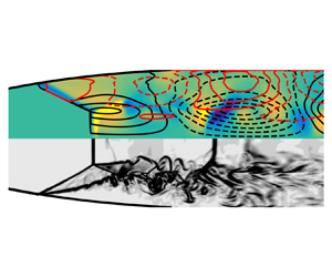
An instantaneous pseudo-schlieren visualization is first presented in figure 4. It shows that the essential expected features of the flow are well reproduced. The open separation here arises from around the middle of the nozzle divergent. The average position of the separation line experimentally observed from pressure data (and confirmed with oil films) at  $x/D=0.93$ nearly coincide with the one numerically evaluated at
  $x/D=0.95$ through wall pressure gradients. The separation produces the so-called separation shock and large Mach disk due to irregular shock reflection at the axis. This structure is followed in the downstream by a supersonic annular mixing layer surrounding a subsonic core and surrounded by the reverse recirculation region close to the wall. The flow reacceleration in the supersonic jet then leads to the formation of a secondary Mach disk here located slightly downstream of the nozzle exit. The mean location and extent of both mixing layers and shock structures downstream of the nozzle exit are in good agreement with experimental data available, as shown in particular with the average streamwise velocity field obtained in figure 5 with a comparison with some reference PIV data from a previous study (Jaunet et al. Reference Jaunet, Arbos, Lehnasch and Girard2017).

Figure 4. Instantaneous pseudo-schlieren visualization of the TIC nozzle jet at  $M_j=2.09$.

Figure 5. Average streamwise velocity field: reference  $x$–
$x$– $y$ PIV data (surrounded by black rectangular box) versus overall numerical prediction. Position of the
  $y$–
$y$– $z$ cross-PIV plane (vertical black and white dashed line).
It is worth recalling that in the present simulation, instabilities naturally develop within the annular mixing layers due to the forcing by the arising global jet oscillations. They first emerge during the numerical transient and are maintained when the flow is established. Numerical flow visualizations reveal that the shock motion is dominated by back-and-forth motion (mode  $m=0$) with irregular precession (mode
  $m=1$) alternately in the clockwise or anticlockwise direction. Phases of more intense tilting and/or distortion of the shock structure are occasionally associated with more significant amplitude of oscillation of the jet column, producing larger and more intense coherent structures travelling in the shear layer. However, the shock oscillations observed never produce a sufficiently important change of the Mach disk curvature to generate large vortices close to the axis downstream of the Mach disk, as it could have been reported in Martelli et al. (Reference Martelli, Saccoccio, Ciottoli, Tinney, Baars and Bernardini2020).
The shear layer instabilities seem to be first slightly delayed, as could be expected, as it could yet be classically observed in the absence of any specific upstream forcing treatment. Downstream of the secondary Mach disk, they admittedly also suffer from an excess of numerical diffusion due to the rapid mesh stretching in the downstream region, chosen to limit the computational cost. By comparison with experimental observations in figure 5, the compression/expansion regions within the annular mixing layer yet appear only slightly shifted downstream of their position as experimentally observed. The maximal differences between numerical predictions and experimental measurements of average streamwise velocity typically also remain limited to less than  $10\,\%$ within the mixing layer region at the location of the cross-PIV plane used in the following to examine further the link between internal and external fluctuations.
A particularly good agreement is observed between numerical results and available experimental wall pressure data within the nozzle. These streamwise distributions of average and root mean square (r.m.s.) wall pressure fields are presented in figure 6. They indicate that the present simulation satisfactorily captures the shock position and the jump of both average pressure level and intensity of pressure fluctuations in this critical region.

Figure 6. Mean (black) and r.m.s. (blue) wall pressure distributions along the nozzle wall.
As detailed in § 4.1, the fluctuating variables can be decomposed into azimuthal Fourier modes (see (4.1)). The power spectral densities (PSD) for the antisymmetric azimuthal Fourier mode  $m=1$ of wall pressure fluctuations is presented in figure 7 for the position
  $x/D=1.25$ to compare with similar data available from the ring located at this position during the experiment. The energy distribution of wall pressure fluctuations in the separation region is classically characterized by a large bump at low Strouhal number, mainly associated with the upstream motion of the shock/separation line system, and contributions at high Strouhal number, associated with coherent structures advected within the jet mixing layer. Even if the signature of the upstream shock/separation line is mainly visible on the first axisymmetric mode
  $m=0$, it has a non-negligible contribution to other modes, including this non-axisymmetric mode
  $m=1$. It is worth noting that the present evaluation of low-frequency content is expected to be less converged with simulation data (acquired during a more limited time duration) while a slight shift of upstream conditions during the experiment is naturally likely to exaggerate the very low-frequency content experimentally evaluated. The under-estimation of high-frequency content of fluctuations during the simulation is also consistent with the observation of the delayed development of turbulence within the mixing layers and the lower resolution of the amplitude of pressure fluctuations radiated from these smallest scales of the flow. However, the most dynamically active scales associated with flow oscillations in the intermediate frequency range appear to be particularly well reproduced. The very particular feature here observed is the presence of the tonal peak of the azimuthal mode
  $m=1$ at
  $St \simeq 0.2$. A value of
  $St=0.216$ is predicted with the present simulation strategy, in rather good agreement with the experimental value of
  $St=0.198$. This indicates that the main global flow behaviour responsible for the tonal behaviour of most interest for the present study is well captured with the present simulation and that its relative importance for generation of lateral forces can be estimated.

Figure 7. Comparison of the experimental and numerical PSD of second azimuthal pressure modes  $m=1$ taken at
  $x/D=1.25$.
As a conclusion, even if the present numerical strategy admittedly leads to a limited representation of the simulated external flow entrainment and far-field jet dynamics, the large scales dynamical features of the jet appear to be satisfactorily reproduced in the whole separated region and close to the nozzle exit, allowing us to conduct a finer analysis of the flow dynamics with confidence.
4. Analysis of unsteadiness
4.1. Global spatial and temporal organization of fluctuating field
In the following, we focus on the physical variables of most interest, including the pressure  $p$, density
  $\rho$ and velocity components in the streamwise
  $u_x$, radial
  $u_r$ and azimuthal
  $u_{\theta }$ directions. The fluctuating field is obtained by subtracting the time-averaged field to each instantaneous field. The spatial organization of this fluctuating field is then characterized by decomposing the vector composed of a subset of any fluctuating physical variable
  $\boldsymbol{q}=(p^{\prime },u_x^{\prime },u_r^{\prime },u_{\theta }^{\prime },\rho ^{\prime })^{\textrm {T}}$ into azimuthal Fourier modes as follows:
 \begin{equation} \boldsymbol{q}_m(x,r,t) = \frac{1}{2{\rm \pi}}\int_0^{2{\rm \pi}} \boldsymbol{q}(x,r,\theta,t) \,\textrm{e}^{-\textrm{i} m \theta} \,\textrm{d}\theta, \end{equation}
where  $m$ is the azimuthal mode number. The features of the fluctuating wall pressure field are first examined. For each ring of wall pressure sensors, the pressure field is thus decomposed into azimuthal Fourier modes according to (4.1). The PSD of the three first modes evaluated at
  $x/D=1.25$ are plotted for example in figure 8. The large low-frequency bump is visible on each distribution. This bump is all the more dominant as we consider a streamwise location close to the separation line and can be associated with the separation shock motion (Jaunet et al. Reference Jaunet, Arbos, Lehnasch and Girard2017). The large dominance of energy for
  $m=0$ close to the separation line suggests that this shock motion mainly remains axisymmetric. Some significant fluctuating energy is also contained in the high-frequency (
 $St > 0.8$) range and increases as we move in the downstream direction. It is attributed to the passage of smaller coherent structures advected along the separated region and jet mixing layer. Their contribution appear rather uniformly distributed in each azimuthal mode. The most salient feature is the presence of a peak of the antisymmetric mode
  $m=1$ at
  $St \simeq 0.2$ in the middle frequency range. It should be recalled that this peak exists for a narrow range of operating conditions but is more particularly dominant for
  $M_j=2.09$. Other peaks at other frequencies can be detected in the other azimuthal modes but remain of significantly lower amplitude.

Figure 8. The PSD of three first azimuthal wall pressure modes at  $x/D=1.25$ (experimental data).
The present analysis is extended to the internal flow region based on numerical data. The PSD of the fluctuating pressure mode  $m=1$ is for example shown in figure 9 for the plane
  $x/D=1.43$ (corresponding to the middle of the open separated region). As expected, some high levels of energy in a wide frequency range are observed between the radial positions
  $r/D=0.2$ and
  $0.25$. This zone corresponds to the mixing layer region spatially developing between the near axis subsonic jet core (downstream of the first internal Mach disk) and the external recirculation region. Whatever the radial position, a peak of energy also clearly emerges at
  $St\simeq 0.2$. This result thus indicates that the particular wall pressure field organization previously observed is not confined to the near-wall region. It rather appears as the signature of a more global flow organization of the pressure field prevailing through the whole separated flow region within the nozzle. The maximal energy levels are located within the mixing layer, more particularly close to the internal part of the mixing layer (at
  $r/D\simeq 0.215$) for this streamwise location. This highlights the probable prominent role of intrinsic non-axisymmetric instabilities spatially developing within the jet mixing layer inside the nozzle.

Figure 9. The PSD map of the azimuthal pressure mode  $m=1$ in the plane at
  $x/D=1.43$ as a function of the radius (numerical data).
The organization of the velocity field downstream of the nozzle exit and its link with the internal wall pressure field are now examined. The structure of velocity field at the position of the PIV plane (i.e.  $x/D = 3.63$) is first briefly described. The overall flow visualization given by figure 5 indicates that a second Mach disk forms just downstream of the nozzle exit and is followed by subsequent expansion/compression zones. The PIV plane is located close to the end of the pseudo-potential core slightly before the internal part of the mixing layer reaches the jet axis. In this region, a deficit of velocity could be still observed near the jet centre in the radial profile of mean streamwise velocity. The mixing region roughly extends from
  $r/D=0.2$ to
  $0.6$. The flow at this location is composed of two distinct mixing regions: (i) an internal mixing layer issued from the triple point connected to the separation shock and first Mach disk within the nozzle and (ii) an external mixing layer between the surrounding supersonic coflow and the recirculation zone. Higher values of r.m.s. velocity are naturally observed in this region with a peak value found near
  $r/D=0.33$, which corresponds to the merging zone between these internal and external mixing layers. As expected for such a position located quite far downstream, the results show that the fluctuating energy within the whole mixing region is distributed into a large number of azimuthal modes and within a large frequency range. However, as shown in figure 10, a small peak still clearly emerges at
  $St\simeq 0.2$ in the PSD of first azimuthal mode of velocity. It is more particularly visible near
  $r/D=0.33$ where the merging between the internal and external mixing layers is observed and where the maximal r.m.s. values are detected. The amplitude of this energy peak of first mode of velocity field is here far lower than the one of first azimuthal pressure mode of the internal wall pressure signals. It remains, however, sufficiently significant to suggest that the turbulent structures spatially developing within the jet mixing layers also exhibit the same signature of a common global oscillation mechanism.

Figure 10. The PSD map of the antisymmetric azimuthal mode of velocity fluctuations (from experimental PIV data), normalized by the fully expanded jet velocity, as function of radius and Strouhal number at  $x/D=3.63$. Amplitudes are plotted using a logarithmic scale.
Synchronized and time-resolved data of wall pressure and external velocity have been obtained during a time period long enough to allow an extended correlation analysis based on experimental measurements. A low-pass filtering of wall pressure data is first applied in order to obtain pressure and velocity signals with similar sample rate. The coherence between the first azimuthal modes of internal pressure at a ring of wall pressure sensors and first azimuthal mode of streamwise velocity is computed. The coherence map obtained remains rather similar whatever the pressure ring position considered. The map obtained for the ring of sensors at  $x/D=0.9$ and the PIV plane at
  $x/D=3.63$ is for example presented in figure 11. As expected, the signals are uncorrelated at nearly all frequencies due to the important distance between the internal sensors and the external velocity plane. However, a significant coherence level emerges at
  $St \simeq 0.2$ and more particularly close to
  $r/D=0.33$ in the external velocity plane and to a lesser extent close to
  $r/D=0.51$. As previously mentioned, this first position corresponds to the zone where the internal and external mixing layers start merging. The second outer position is close to the boundary of the external mixing layer. In spite of high-amplitude and stochastic turbulent fluctuations found within the jet at such a quite far downstream position, the existence of such a peak of coherence reveals that first modes of internal pressure fluctuations and external velocity fluctuations remain significantly correlated but only in a narrow middle frequency range. The non-axisymmetric modes of internal pressure field and the external jet velocity field thus share the common signature of an organized coherent motion in this particular narrow frequency range.

Figure 11. Coherence map between azimuthal modes  $m=1$ of wall pressure signals at
  $x/D=0.9$ and jet velocity at
  $x/D=3.62$ (experimental data).
5. Identification of global coherent jet flow structure
5.1. Coherent structures eduction
In order to explore the coherent structures of the flow, we propose to decompose the flow in orthogonal modes using SPOD. Details of SPOD have been recently discussed in Towne, Schmidt & Colonius (Reference Towne, Schmidt and Colonius2018) and we provide in the following a brief reminder of the processing to introduce the notation.
In order to compute the SPOD modes  $\boldsymbol{\varPsi}$, we first form the cross-spectral density (CSD) matrix
  $\boldsymbol{\mathsf{P}}_{qq}$, at the frequency
  $\omega$, of vector
  $\boldsymbol{q}$ whose components correspond to a chosen subset of fluctuating parts of physical variables of interest. The dominant SPOD modes identified can sometimes differ as a function of the components chosen to build
  $\boldsymbol{q}$. In the present case, it has been checked that considering one single component vector based on the fluctuating pressure or a vector composed of both the pressure fluctuation and fluctuation of the streamwise velocity component leads to similar results. The results shown in the following are obtained based on the two components vector
  $\boldsymbol{q}=(p^{\prime },u_x^{\prime })^{\textrm {T}}$.
  $\boldsymbol{\mathsf{P}}_{qq}$ is computed using Welch's periodogram method,
 \begin{equation} \boldsymbol{\mathsf{P}}_{qq} = E\left\{ \hat{\boldsymbol{q}} \hat{\boldsymbol{q}}^{\boldsymbol{H}}\right\}, \end{equation}
where  $E$ denotes the expectation operator,
  $\hat {\boldsymbol{q}}$ is amplitude of the time domain Fourier transform of
  $\boldsymbol{q}$ at the frequency
  $\omega$,
 \begin{equation} \hat{\boldsymbol{q}} = \sum_t \boldsymbol{q}(t) \,\textrm{e}^{-\textrm{i} \omega t} \end{equation}
and  $\hat {\boldsymbol{q}}^{\boldsymbol{H}}$ is its transpose conjugate. Note that for reasons of clarity, we have dropped the time and space dependence of
  $\boldsymbol{q} = \boldsymbol{q}(\boldsymbol {x},t)$ whenever possible.
Finally, the SPOD modes are obtained by computing the eigenvectors of the CSD matrix,
 \begin{equation} \boldsymbol{\mathsf{P}}_{qq} \boldsymbol{\varPsi} = \boldsymbol{\varPsi} \boldsymbol{\varLambda}, \end{equation}
where  $\boldsymbol{\varLambda} = \textrm {diag}(\lambda ^{(i)})$ is the diagonal matrix of the SPOD eigenvalues sorted in ascending order. Since
  $\boldsymbol{\mathsf{P}}_{qq}$ is Hermitian by construction, all eigenvalues are positive. Here
  ${\boldsymbol{\varPsi}}$ is the matrix whose columns are the individual SPOD modes
  $\boldsymbol{\varPsi} ^{(i)}$ as follows:
 \begin{equation} {\boldsymbol{\varPsi}} = \left[\boldsymbol{\varPsi}^{(1)}, \boldsymbol{\varPsi}^{(2)},\ldots , \boldsymbol{\varPsi}^{(N)} \right], \end{equation}
where  $N$ is the rank of
  $\boldsymbol{\mathsf{P}}_{qq}$.
A low-order reconstruction of the CSD matrix  $\tilde {\boldsymbol{\mathsf{P}}}_{qq}$ can be formed using a subset of
  $N_{tr}$ SPOD modes and eigenvalues,
 \begin{equation} \tilde{\boldsymbol{\mathsf{P}}}_{qq} = \sum_{i=1}^{N_{tr}} \boldsymbol{\varPsi}^{(i)} \lambda^{(i)} {\boldsymbol{\varPsi}^{(i)H}}. \end{equation}
In the following, we focus on the first non-axisymmetric azimuthal mode of the flow fluctuations  $\boldsymbol{q}_m(x,r,t)$ with
  $m=1$, since this is the one supporting most of the dynamics at the frequency of the tonal dynamics. The flow variables are therefore first decomposed into azimuthal Fourier modes, as given by (4.1), prior to computing the SPOD modes, and we retain only the
  $m=1$ mode
  $\boldsymbol{q}_1(x,r,t)$. Note that, for sake of conciseness, we dropped the
  $(\cdot )_1$ subscript for the remainder of the paper.
Since they are based on a two-points statistics of the flow, the computation of SPOD modes requires a large amount of data. In order to control the convergence rate of the decomposition and ensure that the analysis presented in the following sections is relevant, we separate the data in two halves and SPOD modes are computed on each subset. Then, we compute the scalar-product  $\beta$ between the SPOD modes obtained with each of these subsets:
 \begin{equation} \beta = (\boldsymbol{\psi}^{(i)}_1,\boldsymbol{\psi}^{(i)}_2), \end{equation}
where  $(\cdot ,\cdot )$ is the scalar product,
  $\boldsymbol{\psi}^{(i)}_1$ and
  $\boldsymbol{\psi}^{(i)}_2$ refer to the SPOD modes obtained with the first and the second half of the data, respectively.
For a pair of SPOD modes at one given frequency, a scalar product differing from unity reveals the non-similarity between each corresponding mode of each database. The analysis of the spatial support of the mode is likely to be biased in such a case. In the present study, it is indeed found that the original set of snapshots is not large enough to ensure a convergence of the second- and higher-order SPOD modes. Increasing the size of the database with longer simulation times (which was not possible due to computational limits) would be required to improve the convergence rate. The convergence of first SPOD mode, however, seems to be sufficient at the tonal frequency. The scalar product between this first SPOD modes extracted from each half of the database is plotted against frequency for the available frequency range in figure 12. As can be seen, the average scalar product is around  $\beta =0.6$, indicating that even the convergence of the first SPOD mode is not reached for many frequencies. On the contrary, a value very close to unity is measured at the tonal frequency of interest of
  $St \simeq 0.2$. Hence, the SPOD mode at this frequency can be reliably examined. The relative difference of energy content of the other higher modes with respect to the energy of first mode can still be reliably interpreted but their too weak convergence rate a priori inhibits a clear interpretation of their spatial shape which would be likely to evolve by considering more snapshots for the analysis. Only the first mode at the tonal frequency will thus be considered in detail in the following analysis, and the spatial shape of higher modes will not be discussed.

Figure 12. Absolute value of the scalar product  $\beta$ between the first SPOD modes computed with the first half of the data and the ones computed with the second half of the data.
5.2. Dominant SPOD mode
We present in figure 13 the eigenvalues of the SPOD modes as a function of the Strouhal number. The energy content of the first mode clearly dominates the energy content of all the other modes at any frequency (with a ratio varying typically between  $2$ and
  $4$). It is striking that the resonant frequency SPOD modes show a far more important gain separation (of more than one decade) between the first and second SPOD modes. This emphasizes that the tonal dynamics differs in nature from the rest of the spectrum. At the resonant frequency, the first SPOD mode represents more than 80 % of the energy of the flow dynamics. This shows that most, if not all, of the dynamics associated with the resonance has been extracted from the data by the SPOD analysis.

Figure 13. The SPOD eigenvalue as a function of Strouhal number. Darker lines correspond to the more energetic eigenvalues.
The dominant SPOD mode spatial signature at the Strouhal number of the resonance is presented in figure 14. There are several important structures to notice in the spatial support of this SPOD mode. First of all, we recognize inside the nozzle the fingerprint of the adaptation shock structure with its Mach disk within the nozzle. This shows that the shock system motion naturally shares the signature of the dynamics at the resonant frequency. Note that such discontinuities are expected to be excessively highlighted since they impose amplitudes of local pressure and velocity gradients far more important than the one associated with other travelling coherent structures in the flow. Note that the colour palette has been thresholded so as to avoid that these shocks hide the presence of other essential elements of the global structure.

Figure 14. Real part of the first SPOD mode at  $St = 0.216$: pressure (a) and streamwise velocity (b). The amplitude have been normalized by the maximum value and the colour scale is saturated in
  ${\pm }20\,\%$ of this maximum value.
Also visible in the figure is the presence of two distinct large-scale wavepackets. A first inner wavepacket appears partially confined inside the exhaust jet, i.e. for  $r/D < 0.25$, approximately. The second outer wavy pattern is also recognizable beyond the jet boundary for
  $r/D > 0.25$. The presence of these wavy patterns in the SPOD mode structure all along the jet confirms the link previously established between internal and external fluctuations. In order to better identify the possible origin of the tonal behaviour, the propagative properties carried by this SPOD mode are examined in the following section.
5.3. Upstream/downstream propagating waves
Animating this dominant SPOD mode shows that the inner wavepacket possesses wavefronts moving in the downstream direction whereas the outer wavepacket is propagating in the upstream direction. Note that we cannot infer the group velocity of such structures and cannot put directly into evidence that the energy carried by those waves goes in the same directions. The observation of the phase velocity directions of these two wavepackets is, however, already by itself a strong indication of a possible emergence of resonance.
Following the analysis proposed by Edgington-Mitchell et al. (Reference Edgington-Mitchell, Jaunet, Jordan, Towne, Soria and Honnery2018), the essential ingredients composing the dominant SPOD mode at the resonant frequency are further examined by carrying out a Fourier transformation in the streamwise direction,
 \begin{equation} \hat{\boldsymbol{\varPsi}}^{(1)}(k,r) = \sum_x \boldsymbol{\varPsi}^{(1)}(x,r)\,\textrm{e}^{\textrm{i}kx}, \end{equation}
where  $k$ is wavenumber in the streamwise direction. For each radial position, the window considered for the Fourier transform extends from the first available point at the nozzle wall up to the end of the computational domain. We present in figure 15 the amplitude distribution of
  $\hat {\boldsymbol{\varPsi}}^{(1)}(k,r)$. It is evident, from this figure, that the SPOD modes spectrum is dominated by two distinct regions: one in the positive wavenumber domain (
 $k \simeq 0.5$), i.e. with positive phase speed, and the other in the negative wavenumber region (
 $k \simeq -0.7$), i.e. with negative phase speed. This confirms the observations we made while animating the SPOD mode in the time domain.

Figure 15. Fourier transform SPOD mode of pressure at  $St = 0.216$. The amplitude has been normalized by the maximum value and the colour scale is saturated in
  ${\pm }20\,\%$ of this maximum value.
In figure 16(a) we present a filtered version of the previous Fourier spectrum where we have only retained the wavenumbers around the dominating downstream travelling waves. The corresponding pressure waves in the physical domain are plotted in figure 16(b). The streamwise organization of this structure, i.e. growth, saturation and decay, as well as its radial shape, i.e. exponential radial decay, is a strong indication that this structure is similar to a Kelvin–Helmholtz (KH) instability wave. As can be seen in figure 5, the velocity profile downstream of the Mach disk shows two strong gradients at both inner and outer mixing layers, supporting the possible inflectional nature and thus unstable nature of the observed waves. Interestingly, the peak amplitude of this structure is located at the level of the internal mixing layer issued from the triple point downstream of the shock structure, suggesting that this wave is probably generated by a classical inflectional mechanism, but here located in this internal part of the jet. The external part of the shear layer (between the separation line and the impinging point of the reflected shock) is not involved with the wavepackets here identified. These observations thus put forward the role of the internal mixing layer in the resonance mechanism of this over-expanded jet and suggest that the sensitivity zone for the emergence of the resonance is located near the triple point rather than the separation line as suggested in recent studies (Martelli et al. Reference Martelli, Saccoccio, Ciottoli, Tinney, Baars and Bernardini2020). In the rest of the paper, we will use the term KH wave when we refer to this downstream travelling structure.

Figure 16. Positive phase-speed filtered Fourier transform (a) and its inverse (b), of the first SPOD mode of pressure at  $St = 0.216$. The amplitude have been normalized by the maximum value of the original, non-transformed, SPOD mode and the colour scale is saturated in
  ${\pm } 20\,\%$ of this maximum value.
Similarly, in figure 17(a) we present a filtered version of the previous Fourier spectrum where we have only retained the wavenumbers around the dominating upstream travelling waves. The corresponding pressure waves in the physical domain are plotted in figure 17(b). It is evident that most of its energy is located outside of the jet, which makes it an excellent candidate to close the feedback loop of the resonance occurring at this frequency. An important feature to note, is that this coherent structure has some non-negligible signature inside the jet and more particularly within the internal mixing layer. Hence, it is possible that the downstream KH structure and this upstream wave exchange energy near by the adaptation shock triple point, where the KH receptivity is a priori maximum. This slightly contrasts with the conjecture of Martelli et al. (Reference Martelli, Saccoccio, Ciottoli, Tinney, Baars and Bernardini2020) who stated that the loop may be closed at the separation point and shows that other possible paths are possible and should not be discarded. Some more work, outside the scope of the present paper, would be necessary to search for the exact feedback-loop path.

Figure 17. Negative phase-speed filtered Fourier transform (a), and its inverse (b), of the first SPOD mode of pressure at  $St = 0.216$. The amplitude have been normalized by the maximum value of the original, non-transformed, SPOD mode and the colour scale is saturated in
  ${\pm } 20\,\%$ of this maximum value.
Finally, in figure 18(a) we present a filtered version of the previous Fourier spectrum where we have only retained the remaining wavenumbers after subtraction of both the dominating upstream and downstream travelling waves. The corresponding pressure waves in the physical domain are plotted in figure 18(b). It is clear from the figure that the remaining wavenumbers represent the fluctuations associated with the motion of the shock structures (first and second Mach disks) as well as the train of other compression and expansion fans in the supersonic annular mixing layer of the jet column. Although these wavenumbers do not dominate the spatial Fourier spectrum, it shows, as expected, that the shock system responds at the resonance frequency in a very coherent manner.

Figure 18. Remaining filtered Fourier transform (a), and its inverse (b), of the first SPOD mode of pressure at  $St = 0.216$. The amplitude have been normalized by the maximum value of the original, non-transformed, SPOD mode and the colour scale is saturated in
  ${\pm }20\,\%$ of this maximum value.
The later observations allow us to propose a plausible mechanism of the observed resonance, involving a downstream unstable KH instability wave supported by the inner shear layer and an external wave, possessing support inside the core of the jet, to close the feedback loop. This scenario shows some similarity with the recent propositions of Martelli et al. (Reference Martelli, Saccoccio, Ciottoli, Tinney, Baars and Bernardini2020) in the fact that the triple point and the instability of the inner shear layer are of importance for the dynamics of the system, underpinning the conjecture given by Jaunet et al. (Reference Jaunet, Arbos, Lehnasch and Girard2017).
The scenario makes, however, some important differences with the classical screech-like scenario, where the outer shear layer supports both the downstream- and upstream-propagating disturbances (see, for example, Tam et al. Reference Tam, Seiner and Yu1986; Edgington-Mitchell et al. Reference Edgington-Mitchell, Jaunet, Jordan, Towne, Soria and Honnery2018; Gojon, Bogey & Mihaescu Reference Gojon, Bogey and Mihaescu2018; Mancinelli et al. Reference Mancinelli, Jaunet, Jordan and Towne2019). Then, the resonance synchronizes all the jet dynamics, especially the outer shear layer, providing strong enough pressure fluctuations to make the shock system move to adapt to the pressure changes. We provide illustrations of this scenario in figure 19 which is made of the superposition of shock-related fluctuations as coloured contours and upstream-propagating related fluctuations as contour lines of positive and negative values in plain and dashed lines, respectively. As can be seen, negative upstream-mode pressure fluctuations are in phase with positive shock-related fluctuations near by the average separation oblique shock location, corresponding to an upstream motion of the shock in a fixed reference frame. This upstream motion of the shock leads to a weaker shock wave, explaining the diminution of plateau pressure downstream in the nozzle. The opposite observation can be made with positive upstream-propagating disturbances.

Figure 19. Example of pressure fluctuation distributions for an upstream motion of the shock (a) and a downstream one (b). Coloured contours represent the pressure fluctuations associated with shock motions and contour lines represent positive (plain) and negative (dashed) pressure fluctuations associated with the upstream mode.
The present interpretation of the data assumes all perturbations to evolve around the time-invariant mean-flow. This is a very simplified view of the dynamics of the flow where shock motions, for example, may change the flow conditions defining the shapes and growth rate of instability modes in both the external and the internal mixing layers downstream of the Mach disk. However, inflectional instabilities will still be present at any time in the flow, so that the main resonance mechanism, that we propose here, should not be affected too much by the slight mean flow changes.
Since the  $m=1$ mode has both real and imaginary parts by construction, it also possesses a negative frequency content which may differ from its positive counterpart. It has been checked that the same exact conclusions could have been drawn by studying the SPOD mode for the corresponding negative frequency. The positive and negative frequency components actually just describe either the clockwise or the anticlockwise rotation of the azimuthal mode
  $m=1$.
From an engineering point of view, it is important to notice that all of the main structures detailed above have some pressure signature at the wall. Since we are only dealing with the  $m=1$ azimuthal Fourier mode, this means that they all contribute to the generation of side forces. The features of lateral forces associated with the resonance mechanism are more precisely described in the following section.
6. Lateral pressure forces
6.1. Description of wall pressure forces
The aerodynamic forces resulting from the particular flow organization previously described are now examined based on the numerical data.
The time evolution of the global force integrated all along the nozzle divergent is computed to examine the resulting spectral properties of each force component. The PSD of each force component is reported in figure 20. The hump around  $St=0.07$ in the PSD of
  $F_{x}$ can be related to the global axisymmetric motion of the upstream separation line. It should be remembered that rather low-frequency contributions to lateral forces are more often reported in other studies corresponding to separated jets without any clear tonal behaviour. Such low-frequency components are thus often associated only with dominant low-frequency shock motions for all modes. The most original observation in the present study is the emergence of the dominant peak also for lateral forces around
  $St \simeq 0.2$. This result thus contrasts with other results in the literature. Only moderate fluctuating energy levels of pressure mode
  $m=1$ are indeed observed locally within the flow. However, their coherence in the streamwise direction appears sufficiently important to lead to a dominant contribution to lateral forces. It should be noted that the amplitude of lateral forces at the tonal peak is even higher than the amplitude of thrust oscillations in the present case.

Figure 20. The PSD of normalized aerodynamic forces acting on the nozzle in the axial direction  $F_{x}$ and radial direction
  $F_{r}$.
6.2. Origins of lateral wall pressure forces
Following Dumnov (Reference Dumnov1996), the side-loads PSD,  $F_\omega$, is the Fourier transform of the time-domain autocorrelation function,
 \begin{equation} F_{\omega} = \iint_{-\infty}^{\infty} F(t)F^*(t+\tau)\, \textrm{d}t \, \textrm{e}^{-\textrm{i}\omega\tau} \,\textrm{d}\tau. \end{equation}
It is then straightforward to show that  $F_\omega$ is related to the first azimuthal mode of nozzle wall pressure,
 \begin{equation} F_\omega = 4{\rm \pi}^2 \int_{0}^L \int_0^L r(z) r(x) \boldsymbol{\mathsf{P}}_{1,\omega}(x,z)\,{\textrm{d}x} \, \textrm{d}z, \end{equation}
where
 \begin{equation} \boldsymbol{\mathsf{P}}_{1,\omega}(x,z) = \iint_{-\infty}^{\infty} \boldsymbol{p}_1(z,t) \boldsymbol{p}^*_{1}(x,t+\ \tau) \, \textrm{d}t \,\textrm{e}^{-\textrm{i}\omega\tau} \,\textrm{d}\tau, \end{equation}
is the CSD of the antisymmetric azimuthal Fourier mode  $m=1$ of the wall pressure fluctuation
  $\boldsymbol{p}_1(x,t)$. As already mentioned by Dumnov (Reference Dumnov1996), the side-loads PSD can only be obtained with a full knowledge of the wall pressure CSD. This two-point statistics can still only be obtained through numerical models.
Taking advantage of the space–time discretization of the domain, the side-loads formula (6.2) at the frequency  $\omega$ can be written in matrix form as
 \begin{equation} F_\omega = \boldsymbol{w}^{\textrm{T}} \, \boldsymbol{\mathsf{P}}_{1,\omega} \,\boldsymbol{w}, \end{equation}
where  $\boldsymbol {w}$ is a column vector of size corresponding to the number of discretization points at the wall, containing the integral weights:
  $\boldsymbol {w} = 2{\rm \pi} L \boldsymbol {\cdot } \boldsymbol {r}$. The CSD matrix of the antisymmetric wall pressure is computed using Welch's periodogram technique,
 \begin{equation} \boldsymbol{\mathsf{P}}_{1,\omega}= E\left\{ \hat{\boldsymbol{p}}_{1,\omega} \hat{\boldsymbol{p}}_{1,\omega}^H\right\}, \end{equation}
where  $E\{\cdot \}$ is the expectation operator. Similarly to what has been done previously, the coherent structure acting on the wall can be obtained by decomposing the wall pressure CSD matrix into SPOD modes,
 \begin{equation} F_\omega = \boldsymbol{w}^{\textrm{T}} \; \boldsymbol {\varPhi }_\omega \boldsymbol{\varTheta}_\omega \boldsymbol{\varPhi }^H_\omega \; \boldsymbol{w}, \end{equation}
where  $\boldsymbol {\varPhi }$ is the matrix formed whose columns are the SPOD modes vectors and
  $\boldsymbol{\varTheta} = \textrm {diag}(\theta )$ is the matrix of eigenvalues. This SPOD analysis only focuses on the wall pressure fluctuation, which is different from the previous analysis where we considered the entire fluid domain. There is no evidence, a priori, that both analyses lead to identical features of coherent structures at the wall. This formulation is interesting because we can form a low rank side-loads amplitude by considering a truncation of the CSD using, for example, the
  $N$ most energetic SPOD modes,
 \begin{equation} F_\omega \geq \boldsymbol{w}^{\textrm{T}} \left( \sum_{i=1}^N \boldsymbol{\phi}^{(i)}_\omega \theta^{(i)}_\omega \boldsymbol{\phi}^{(i)H}_{\omega} \right) \; \boldsymbol{w}. \end{equation}
In case the wall pressure fluctuation possess a low rank dynamics, i.e.  $\theta ^{(1)} \gg \theta ^{(2)}$, the first SPOD mode of the wall pressure is responsible for the majority of the off-axis forces.
As for the analysis of the global field, the convergence of this SPOD analysis of wall fluctuating pressure field has been checked and similar observations are made. The eigenvalues are plotted in figure 21 as a function of the Strouhal number. As can be seen, the first SPOD mode dominates the dynamics to the wall pressure fluctuations for a wide range of frequencies, but even more at the resonance frequency  $St\simeq 0.2$, where a difference of almost two orders of magnitude can be found between the first and the second SPOD eigenvalues.

Figure 21. The SPOD eigenvalues of the wall pressure signature as a function of Strouhal number.
The spatial distribution of the dominant SPOD mode of wall pressure fluctuations at the resonance frequency ( $St=0.216$) is shown in figure 22. As expected, the structure of this SPOD mode is characterized by a peak at the separation shock foot (
 $x/D \simeq 0.9$). This is coherent with the early side-loads generation scenario, proposed by Schmucker (Reference Schmucker1973a), involving asymmetric position of the separation point. From the results of figure 22, we can see, however, that in the separated region, downstream of the shock, the pressure fluctuations are also almost as high as the shock associated ones. This confirms, as proposed by Dumnov (Reference Dumnov1996) and more recently by Aghababaie & Theunissen (Reference Aghababaie and Theunissen2015) in their dynamical model, the significant role of the separated region in the side-loads generation.

Figure 22. Comparison of wall pressure SPOD modes with the wall signature of global SPOD modes. The SPOD modes are normalized with respect to their maximum value in the plotted range.
The wall pressure fluctuation associated with the global coherent structure found in the flow at the resonant frequency (see figure 14) is also reported in figure 22. It is striking that both the coherent wall pressure fluctuation and the wall pressure signature of the global coherent structure, identified earlier, collapse almost perfectly. This is evidence that the global coherent structure, found in the jet flow, is responsible for most of the wall pressure fluctuations, and thus side-forces in the present case where a resonance emerges. From a general point of view, this shows that the shock motion and the separated region dynamics are not the only ingredients in the generation of side forces. It is clear from these results that the exiting jet flow dynamics also contributes and may not be neglected in side-loads modelling efforts.
We have shown that the jet flow coherent structure is responsible for the side-loads creation at the resonance frequency. Since we have previously shown that several distinct waves compose the structure of this coherent structure, i.e. the KH wave, the external wave and the shock related structure, we would like to further investigate the role of each of these individual components onto the generation of side-loads. To this aim, the contribution of each filtered dominant SPOD mode (see figures 16–18) is computed as follows:
 \begin{equation} \tilde{F}_{\omega} = \boldsymbol{w}^{\textrm{T}} \left( \boldsymbol{\tilde{\psi}}^{(1)}_\omega \theta^{(1)}_\omega \boldsymbol{\tilde{\psi}}^{(1)H}_{\omega} \right) \; \boldsymbol{w}. \end{equation}
Indeed, the superposition of the individual contributions of the dominant SPOD mode filtered based on different spatial wavenumbers can be constructive or additive, i.e.  $F_\omega \neq \sum \tilde{F}_\omega$, nevertheless, their relative importance can be of interest in aiming at understanding the side-loads generation mechanism. We present in figure 23 the wall pressure signature of the downstream wave, the upstream one and the shock structure motion. It is clear that most of the wall pressure signature is related to the shock motion. This represents around 80 % of the side-loads amplitude at that frequency. The other two waves contribute less but still in a non-negligible manner: the downstream and the upstream waves represent around 7 %, and 13 %, respectively, of the off-axis forces.

Figure 23. Comparison of absolute values of wall pressure signature of the total SPOD mode with its individual components, filtered on spatial streamwise wavenumbers corresponding to downstream (KH) travelling waves, upstream travelling waves or remaining (shock) contributions. The SPOD mode contributions are normalized with respect to the maximum value of the total SPOD mode. Destructive interactions between components provides lower ‘total’ than shock-related component around  $x/D=1.5$.
Analysis of the shock related motion of the SPOD modes shows that the separation shock motion and the wall pressure in the whole separation region are indeed correlated. This behaviour corroborates the propositions of Dumnov (Reference Dumnov1996) regarding the main origins of side forces in separated nozzle flows. Our findings, however, suggest that 20 % of the side loads can be discarded when only the shock motion is accounted for.
The presented results are, in the authors’ opinion, a strong indication that the resonance is formed via some sort of feedback loop involving an internal downstream propagating wave and an external upstream propagating one. The shock system reacts in order to adapt to these strong, resonating, pressure fluctuations (as presented in figure 19), therefore creating most of the side forces. The exact nature of the waves at play in the resonance mechanisms, and the identification of the conditions allowing their emergence, deserve some attention in order to fully understand the origins of such a resonance. This issue should be addressed in future studies.
7. Conclusions and perspectives
The dynamical features of a separated supersonic jet in a TIC nozzle have been investigated for a nozzle pressure ratio corresponding to wall pressure oscillations of maximal amplitude. The wall pressure field shows signs of a particular tonal behaviour which has been previously reported. This study has focused on a new correlation analysis of synchronized time-resolved external velocity and internal wall pressure data to further understand the possible link existing between internal and external disturbances. In a narrow frequency band, a significant coherence level has been found between the antisymmetric internal wall pressure oscillations prevailing in the nozzle and antisymmetric external velocity disturbances spatially evolving in the jet mixing layer quite far downstream of the nozzle exit, underpinning the importance of the exiting jet plume dynamics in the nozzle wall pressure suggested in recent studies (Jaunet et al. Reference Jaunet, Arbos, Lehnasch and Girard2017). The flow behaviour has been numerically reproduced by DDES and validated with the available experimental results, allowing a detailed analysis of the resonant dynamics and an evaluation of the subsequent lateral forces applying to the nozzle. It has been shown, thanks to the use of a SPOD analysis, that the resonance is more likely due to a feedback loop involving a downstream propagating wave and an upstream propagating wave, similar to a screech resonance, but rather supported by the internal shear layer issued from the triple point. The present observations have not indicated any evidence of the need of instantaneous Mach disk curvature to sustain the feedback loop of the resonance, as recently proposed by Martelli et al. (Reference Martelli, Ciottoli, Saccoccio, Nasuti, Valorani and Bernardini2019). The specific organization of the over-expanded mean flow, i.e. an annular supersonic jet, makes the downstream waves mostly supported by the inner shear layer issued from the Mach disk triple point. This is a major difference from the usual screech scenario, where both the upstream and downstream waves are supported by the same shear layer (Edgington-Mitchell et al. Reference Edgington-Mitchell, Jaunet, Jordan, Towne, Soria and Honnery2018; Gojon et al. Reference Gojon, Bogey and Mihaescu2018; Mancinelli et al. Reference Mancinelli, Jaunet, Jordan and Towne2019). The present analysis could not indicate the reason for the occurrence of such resonance in over-expanded flows. Some research efforts need to be pursued to clarify the characteristics of the waves involved and the end conditions that make them interact (Jordan et al. Reference Jordan, Jaunet, Towne, Cavalieri, Colonius, Schmidt and Agarwal2018; Mancinelli et al. Reference Mancinelli, Jaunet, Jordan and Towne2019). This would allow us to model and predict the occurrence of those undesirable tonal behaviours. Despite a relatively moderate local energy level of the first azimuthal mode of wall pressure in this frequency range, it has been shown that these tonal jet oscillations fully dominate the whole dynamical behaviour of these lateral forces. The examination of the relative importance of the waves involved in the resonance in the generation of side forces has shown that a non-negligible 20 % of the side forces can be attributed to the resonant waves. The remaining 80 % are shown to be attributed to the motion of the separation shock, but itself induced by the resonance. These findings clearly suggest that the sole shock motion is insufficient to explain and model the side-forces amplitude in a general framework and that the jet flow dynamics should not be discarded in this respect. The results of the present study also indicate that any modification of the exiting jet environment is likely to affect not only the intrinsic external jet dynamics but also the side-loads features.
Funding
Part of the present work has been carried out during the PhD thesis work of Florian Bakulu, supported by CNES and Région Poitou-Charentes. This work was granted access to the HPC resources of TGCC under allocations A0012A10017 made by GENCI.
Declaration of interests
The authors report no conflict of interest.


