


1. Introduction
Laminar flows with recirculation cells are of interest since the residence time of fluid particles in these zones is larger than that in other flow regions. Many practical applications such as stirring and mixing, blood coagulation or bacterial growth depend on this time (Tuval et al. Reference Tuval, Cisneros, Dombrowski, Wolgemuth, Kessler and Goldstein2005; Hathcock Reference Hathcock2006; Cremer et al. Reference Cremer, Segota, Yang, Arnoldini, Sauls, Zhang, Gutierrez, Groisman and Hwa2016). When the flow field is steady, one can identify particle paths with streamlines and easily determine what the global behaviour of fluid particles will be. But when the flow field is unsteady, gaining an insight into the motion of fluid elements becomes non-trivial and fluid particles that are initially close together may largely separate over time. Mixing of fluid particles in laminar flows may rely either on molecular diffusion or on advection (Villermaux Reference Villermaux2019). The value of the Péclet number establishes whether molecular diffusion has a significant role in the mixing process. The terminology regarding mixing and stirring is not always consistent in the literature. We hereafter reserve the term ‘mixing’ to denote diffusion (either molecular or eddy diffusion) and use the term ‘stirring’ to refer to advection. For flows with high-valued Péclet numbers, such as liquids, it is not unusual to find that advection is the prevalent process, and stirring mainly determines the uniformization of initially segregated constituents. With negligible or null diffusion, the stirring properties of two-dimensional laminar cellular flows include the possible existence of persistent barriers to transport. Such flow separators are associated with ‘Lagrangian coherent structures’, which define sets of fluid particles that are minimally dispersive and that move together quite robustly. Lagrangian coherent structures are known to separate dynamically distinct regions in fluid flows (Kelley, Allshouse & Ouellette Reference Kelley, Allshouse and Ouellette2013).
Distinguishing types of behaviour from data is possible using a technique called BraMAH (branched manifold analysis through homologies). Recently used in Charó, Artana & Sciamarella (Reference Charó, Artana and Sciamarella2020) to analyse particle trajectories, it is important to stress that the technique is a general time series analysis method that can be applied to any dynamical system and not only to chaotic regimes. The first attempts to discern the main features of a dynamical system from observational or experimental data date back to Packard et al. (Reference Packard, Crutchfield, Farmer and Shaw1980), who addressed the problem of using time series to reconstruct a finite-dimensional phase-space picture of the sampled system's time evolution using an embedding, and to characterize it geometrically. Data-embedding techniques are used by experimentalists to reconstruct dynamical information from time series (Sauer, Yorke & Casdagli Reference Sauer, Yorke and Casdagli1991). The advantage of using topological instead of geometrical properties to describe embedded data lies in the fact that the former provide information about the mechanisms that act in phase space to construct the flow. These mechanisms – stretching, squeezing, tearing, folding – are topological in nature, and they are intimately related to the governing equations (Birman & Williams Reference Birman and Williams1983). In the case of a fluid particle, the coordinates of the particle position span a subspace of phase space. Restricting the characterization of the dynamics of a fluid particle to the subspace spanned by the position coordinates may be problematic, as discussed in Charó et al. (Reference Charó, Sciamarella, Mangiarotti, Artana and Letellier2019). It is therefore advisable to work with embeddings involving as many dimensions as necessary, i.e. without projecting the data onto a lower-dimensional space.
Specific implementations have been proposed to extract topological features from time series: the first ones were based on the way in which the unstable periodic orbits in phase space are knotted among themselves (Mindlin et al. Reference Mindlin, Hou, Solari, Gilmore and Tufillaro1990, Reference Mindlin, Solari, Natiello, Gilmore and Hou1991), but this approach was restricted by the phase-space dimension which could not be higher than three – since knots unknot in more than three dimensions – and by the possibility of identifying periodic orbits within a time series, i.e. nearly periodic data portions to which the method of close returns (Lathrop & Kostelich Reference Lathrop and Kostelich1989) can be applied, in order to reconstruct the unstable periodic orbits from a set of points in an embedding from experimental measurements. This required long and almost noise-free time series. In order to overcome these difficulties, tools from algebraic topology were proposed (Muldoon et al. Reference Muldoon, MacKay, Huke and Broomhead1993; Sciamarella & Mindlin Reference Sciamarella and Mindlin1999, Reference Sciamarella and Mindlin2001; Maletić, Zhao & Rajković Reference Maletić, Zhao and Rajković2016). Natiello et al. (Reference Natiello2007) typify this approach as ‘knotless’ and periodic ‘orbitless’, ‘since the data is characterized as a whole, regardless of the existence of hidden periodic orbits in it’. In this sense, BraMAH is an orbitless and knotless method that is specifically designed to compute topological properties enabling the identification of (branched) manifolds from a cloud of points in phase space. The resulting manifold may have branches or not: no a priori assumptions are made, since the aim of the approach is to discern the nature of the dynamics from observations, unaided by previous knowledge of the system's properties.
A cautionary note on language is necessary, since there are many terms that are shared between fluid mechanics and dynamical systems theory, and that may lead to ambiguities. The words ‘trajectory’ or ‘flow’ are common to both domains. Trajectories in fluid mechanics refer to particles flowing in a fluid in a physical space that cannot be higher than three-dimensional, while trajectories of a flow in phase space can be of any dimension since they refer to solutions of an equation system for a set of initial conditions. For the sake of clarity, we always indicate to which type of space we are referring.
This work describes the application of this technique to the numerically generated particle trajectories in a fluid flow past an oscillating cylinder, and compares it with the results obtained for a paradigmatic analytical model of Lagrangian motion (Shadden, Lekien & Marsden Reference Shadden, Lekien and Marsden2005). In the particular context of Lagrangian studies, the approach adopted here can be framed within a class of methods that measure complexity of individual particle trajectories in order to identify or ‘colour’ regions with qualitatively different dynamical behaviour of particle trajectories in fluid flows. More specifically, Rypina et al. (Reference Rypina, Scott, Pratt and Brown2011) proposed the use of correlation dimension, ergodicity defect or arclength of individual particle trajectories as a measure of trajectory complexity to identify Lagrangian coherent structures. Mendoza, Mancho & Wiggins (Reference Mendoza, Mancho and Wiggins2014) also proposed the use of arclength or pathlength of individual trajectories to find Lagrangian coherent structures (‘Lagrangian descriptors’ method), while Schlueter-Kuck & Dabiri (Reference Schlueter-Kuck and Dabiri2017) resorted to graph theory proposing a metric of kinematic dissimilarity. Non-individual particle strategies generally rely on the analysis of large sets of particles that must in addition lie initially close to each other. We should of course mention the widely used finite-time and finite-size Lyapunov exponents (Karrasch & Haller Reference Karrasch and Haller2013; Allshouse & Peacock Reference Allshouse and Peacock2015b), variational approaches such as that of Farazmand & Haller (Reference Farazmand and Haller2012), Lagrangian averaged vorticity deviation and diffusive barriers (Haller et al. Reference Haller, Hadjighasem, Farazmand and Huhn2016; Haller, Karrasch & Kogelbauer Reference Haller, Karrasch and Kogelbauer2018), transfer operator methods (Froyland Reference Froyland2013; Froyland & Padberg-Gehle Reference Froyland and Padberg-Gehle2015; Williams, Rypina & Rowley Reference Williams, Rypina and Rowley2015), the encounter volume method (Rypina & Pratt Reference Rypina and Pratt2017; Rypina, Llewellyn Smith & Pratt Reference Rypina, Llewellyn Smith and Pratt2018) and spectral clustering (Hadjighasem et al. Reference Hadjighasem, Karrasch, Teramoto and Haller2016; Vieira, Rypina & Allshouse Reference Vieira, Rypina and Allshouse2020; Filippi et al. Reference Filippi, Rypina, Hadjighasem and Peacock2021), among others.
Complementary strategies can be used to provide alternative visualizations, in order to confirm the results offered by Lagrangian approaches. These include, for instance, tracer release experiments or stroboscopic sections in Navier–Stokes simulations. The latter may require integration over very long times (Rypina et al. Reference Rypina, Pratt, Wang, Özgökmen and Mezic2015), and they may lead to different interpretations according to the initial placement of the markers (Soulvaiotis, Jana & Ottino Reference Soulvaiotis, Jana and Ottino1995). Partial evidence of the presence of transport barriers can sometimes be obtained having recourse to streaklines, i.e. to the instantaneous loci of all the fluid particles that have passed through a particular spatial point in the past, the injection point. Producing streaklines amounts to conducting an experiment in which dye is continuously released from a single or from multiple injection points. In the laboratory, the technique can be easily implemented and is often used to visualize flow patterns, in order to develop flow control strategies (Roca et al. Reference Roca, Cammilleri, Duriez, Mathelin and Artana2014) or to analyse mixing (Balasuriya Reference Balasuriya2017). Streaklines are especially relevant because they can be assumed to correspond to what is observed in a naturally occurring event, such as an oil spill, if diffusion and other processes (weathering or chemical reactions) are neglected. Streakline patterns depend of course on the injection point(s), on the injection time window, on the nature and motion of the transport barriers with respect to the injection point(s), as well as on the molecular diffusion properties of the tracer. If the molecular diffusion of the tracer is negligible, and if the transport barriers move without ever passing through the injection points, streaklines end up indicating the existence of particle-trapping regions in a fluid after a certain ‘buffering time’. In the streakline numerical experiments shown in this study, molecular diffusion of the tracer is neglected, and the location of the injection point(s) is chosen in order to verify that dye is confined by the transport barriers in the way anticipated by the topological analysis.
The cylinder wake has been studied in hundreds of papers due to its scientific and engineering significance (Williamson Reference Williamson1996). The flow configuration adopted here is a case for which vortex shedding is absent and corresponds to low values for the Reynolds number and the rotation parameter. Taneda (Reference Taneda1978) reported experimental studies of such flows, but most of the subsequent research focused upon flows with relatively large Reynolds number, for which vortex shedding was usually observed (Zdravkovich Reference Zdravkovich1997; Choi, Choi & Kang Reference Choi, Choi and Kang2002; Thiria, Goujon-Durand & Wesfreid Reference Thiria, Goujon-Durand and Wesfreid2006). In the case discussed in this work, a moving wall imposes a dynamics in the recirculation region. Numerical simulations show the formation of coherent sets within the recirculation bubble that, to the best of our knowledge, have not yet been reported. This system is dubbed the rotary oscillating cylinder (ROC) system. The coherent regions that are formed are shown to share many features with those formed in the driven double gyre model, dubbed DDG. The topological finite-time analysis conducted in this work will shed further light on the similarities between the ROC and the DDG systems.
The article is organized as follows. Section 2 addresses the main principles for particle topological colouring. Section 3.1 presents the topological finite-time analysis of particle trajectories that are obtained by numerically integrating the Navier–Stokes equations in the ROC system. Section 3.2 revisits the DDG model, showing the results of topological colouring in this reference case. A comparative study is provided in § 4, and conclusions are drawn in the final section. Appendices concerning technical and mathematical questions are provided for completeness.
2. Method
The connection between the topology of dynamical reconstructions in phase space and the transport properties of a fluid flow in physical space is supported by the fact that Lagrangian coherent structures separate dynamically distinct regions (Kelley et al. Reference Kelley, Allshouse and Ouellette2013). The methodology will of course be successful insofar as such coherent sets can be effectively discerned in terms of topologically non-equivalent dynamics in reconstructed phase space. When reconstructed from a time series, the phase space is only partly reconstructed, i.e. only the part of the space visited by the trajectory is reconstructed. Results will therefore be relative to the temporal window that is inspected. A short-term analysis will thus not necessarily coincide with a longer-term analysis. ‘Projection’ effects could also occur due to a poor observability by the variable measured. Recently, tools offering the possibility of numerically assessing the observability of a variable from experimental data have been proposed (Gonzalez et al. Reference Gonzalez, Lainscsek, Sejnowski and Letellier2020). These caveats should be taken into account when interpreting the results.
The starting point of the analysis is a scalar time series of a Lagrangian variable  $\xi$, i.e. a variable that is measured following the fluid particle in its motion. Time series of quantities that are transported by the particle, such as temperature, pollutant concentration, plankton density, etc., may also be considered (Balasuriya, Ouellette & Rypina Reference Balasuriya, Ouellette and Rypina2018), but here we will stick to the problem of examining variables that are fully locked to a particle, leaving this question for future work. Even if BraMAH has the virtue of dealing with relatively short and noisy time series (with respect to knot-theory-based methods), a number of minimal requisites are necessary for any topological finite-time analysis to be fertile. As mentioned before, the length of the time window has an important role in a finite-time analysis. The practical guideline provided in Gilmore (Reference Gilmore1998) is to take more than 20 pseudo-periods, but this number is only indicative and cannot be taken as general. Clearly, the higher the sampling rate, the finer the description. Data may be interpolated or smoothed, but smoothing data from a few points per pseudo-period is very risky, and an over-simplification of the dynamics may be expected.
Some kind of embedding technique is necessary to implement the dynamical reconstruction. We have chosen to work with time-delay embeddings, but differential embeddings as used for global modelling are a possible alternative (Mangiarotti et al. Reference Mangiarotti, Coudret, Drapeau and Jarlan2012). The procedure maps the input time series  $\xi (t)$ into an
  $m$-dimensional space
  $(\xi (t),\xi (t-\tau ), \ldots ,\xi (t-(m-1)\tau ))$. The time delay
  $\tau$ and the embedding dimension
  $m$ are two parameters that must be found in each case. There is no ‘gold’ technique for assessing the optimal time delay (Abarbanel & Gollub Reference Abarbanel and Gollub1996). The rationale is that delay coordinates are correctly chosen if they are sufficiently independent but not uncorrelated. Redundancy is the price to pay if
  $\tau$ is too small, and irrelevance if
  $\tau$ is too large. Standard autocorrelation techniques are ruled out because they only measure the linear dependence of two variables. Their nonlinear counterpart is the average mutual information (AMI) technique, a heuristic approach based on the Shannon entropy (Fraser & Swinney Reference Fraser and Swinney1986; Kantz & Schreiber Reference Kantz and Schreiber2004). For a histogram of resolution
  $\epsilon$, let
  $p_i$ denote the probability of the signal taking a value inside the
  $i$th bin of the histogram. Let
  $p_{ij}$ be the probability that
  $\xi (t)$ is in
  $i$ and
  $\xi (t+ \tau )$ in
  $j$. With these definitions, the mutual information for a time delay
  $\tau$ is given by
 \begin{equation} I_\epsilon(\tau)=\sum_{i,j} p_{ij}(\tau) \ln p_{ij}(\tau) - 2 \sum_{i} p_{i} \ln p_{i}. \end{equation}
The value of  $I_\epsilon (\tau )$ will decrease with
  $\tau$ more or less rapidly, and present afterwards either a slower decay or a set of local minima/maxima. In the first case, the optimal
  $\tau$ is defined by the value at which the first substantial decrease ceases. In the second case, it is the first minimum that is supposed to mark the optimal delay for the embedding. The reliability of the results will, however, depend on the system investigated. The determination of
  $m$ is often done with the method of false nearest neighbours (FNNs) (Kennel, Brown & Abarbanel Reference Kennel, Brown and Abarbanel1992; Abarbanel & Gollub Reference Abarbanel and Gollub1996; Kantz & Schreiber Reference Kantz and Schreiber2004). The FNN method searches for points which are close to each other in a certain embedding space, not because of the dynamics but because the data are projected onto a too low-dimensional space. Given one point and its closest neighbour in
  $m$ dimensions, one computes the ratio of the distances between them in
  $m+1$ dimensions. When
  $m$ has been increased to a value for which no more FNNs are detected, the correct embedding dimension is identified. For noisy data, the proportion of FNNs never drops to zero (Abarbanel & Gollub Reference Abarbanel and Gollub1996), but an appropriate threshold can be chosen. Both parameters
  $m$ and
  $\tau$ will here be determined using the algorithms provided in Ruskeepää (Reference Ruskeepää2017). At the end of this first stage of the process, an
  $m$-dimensional cloud of points is obtained that is associated with a single fluid particle in a specific time window.
Before proceeding to the next step of the method, let us succinctly clarify why the topological study is conducted in a multidimensional working space instead of using the so-called extended phase space, which is three-dimensional, for the behaviour of a particle in a two-dimensional fluid. When a dynamical system is non-autonomous, the phase space is not completely determined, i.e. some processes involved in the dynamics are not explicitly described. The so-called augmented or extended phase space corresponds to setting  $\dot {t}=1$ as if
  $t$ were a dependent variable in the set of governing equations. This way of rewriting the system as an autonomous one is in fact deceitful, since it assigns a double status to the time variable, which is defined as the sole independent variable in dynamical systems theory. Among other problems, this leads to an unbounded phase space where some tools from nonlinear dynamical systems theory do not necessarily apply. The point is discussed in a separate work (Charó et al. Reference Charó, Sciamarella, Mangiarotti, Artana and Letellier2019). Relying instead on sufficiently high-dimensional embeddings helps to avoid projection effects and to achieve better dynamical reconstructions.
The next step is to apply BraMAH to the  $m$-dimensional cloud of points obtained in the embedding stage. The algorithmic procedure and the algebraic topology definitions that are necessary to describe this in detail are provided in Appendices A and B. To give the reader a brief summary of the process, the rationale is the following. The cloud of points is first decomposed into groups of points which will play the role of building blocks, here called cells. Each cell represents a point subset that constitutes a good local approximation of a
  $d$-disk with
  $d \le m$. Notice that
  $d$ is not assumed but calculated as part of the cell construction process. One does not need to set
  $d$ or to know its value in advance. The cells are glued together into a cell complex, which can be thought of as a rough skeleton of the structure upon which the
  $m$-dimensional cloud of points lies. This structure may correspond to an underlying attractor, an invariant manifold or a semi-flow on a broader class of objects that are neither attractors nor manifolds (Muldoon et al. Reference Muldoon, MacKay, Huke and Broomhead1993). The cell complex construction procedure is in fact designed to approximate a cloud of points which is possibly lying on a branched manifold, i.e. a manifold with branches – even if the manifold may have no branches at the end of the process. A cell complex constructed in this manner (with these rules) will be called a BraMAH complex. Once the cell complex is constructed, homology groups can be computed in order to characterize its basic topology. Homology groups are a set of ‘layered’ results which condense the main topological features of the cloud of points: the so-called
  $0$-holes or generators of
  $H_0$ refer to connected components, the
  $1$-holes or generators of
  $H_1$ to the number of holes (a
  $1$-hole is a ‘void’ of dimension
  $1$) and higher-dimensional holes (such as cavities, which are
  $2$-holes or ‘voids’ of dimension
  $2$). In the case of the Lorenz 63 butterfly, for example, there is only one
  $0$-hole, two
  $1$-holes and zero higher-dimensional holes.
Merely counting the different types of holes amounts to computing the Betti numbers, defined as the rank of the homology groups of a cell complex. But the Betti numbers alone do not suffice to identify a branched manifold from a cloud of points. This is why BraMAH explicitly outputs much more information than conventional homology computation methods. The constructed cell complex, whose cells have vertices that are associated with a few points in the original cloud of points, is part of the output, and can therefore be visualized by plotting it, for instance, in juxtaposition with (a three-dimensional projection of) the  $m$-dimensional cloud of points. Note that the computational process used to build the cell complex does not imply projections of any kind; projections are just used to visualize results corresponding to datasets in more than three dimensions. The generators of the homology groups which identify the holes are also part of the output, and are expressed as chains of cells labelled in terms of the vertices. This allows use of the
  $1$-holes to locate the branches, if there are many, and to see how they are relatively disposed or inserted. Torsion information, which is not contained in the homology groups, is retrieved through the computation of two extra features: orientability chains and weak boundaries. Together with Betti numbers, these features are used to define a topological class and therefore to identify a certain type of dynamics with a colour. This means that if the cell complex corresponds to a Klein bottle, as for instance in (Mindlin & Solari Reference Mindlin and Solari1997), BraMAH will detect it correctly. It is important to be aware that a BraMAH cell complex is faithful to the structure of the
  $m$-dimensional cloud of points used as input for the calculation.
In view of the previous statements, the results of a topological finite-time analysis are relative to the variable chosen for the dynamical reconstruction  $\xi (t)$, to the time window (initial time
  $t_w$ and length
  $T_w$) and to the embedding parameters (delay
  $\tau$ and dimension
  $m$). Let us suppose that the position of a limited set of particles is available for the analysis, with startup positions that may of course be sparse. The BraMAH analysis of each particle will yield a topological class. Assigning a colour to each topological class, each particle of the set can be tagged with the colour obtained from its finite-time BraMAH analysis. This operation will be termed topological colouring of fluid particles. By plotting the particles in motion carrying their topological colour, a live picture is obtained of where particles sharing the same colour are located, and how they move. The fact that the same topological classes may appear in different fluid flows may be used to relate dynamical features of fluid particles in different flow configurations. This should, however, be done with care, since a comparison between finite-time topologies in different fluid flows will require the parameters of the analysis to be comparable in the two problems.
3. Results
This section presents the application of the topological finite-time analysis to two cellular flows that present particle-trapping regions. The first subsection considers the recirculation cells in the near wake of the ROC flow from Navier–Stokes numerical simulations. Dynamically distinct zones are identified through the topological colouring of a limited set of particles advected in the numerically solved flow field. As mentioned in the introduction, streaklines are used as an alternative visualization strategy to confirm the results obtained through the topological analysis.
The second subsection presents the same operation with the DDG flow, an analytical system with a lateral forcing that produces an effect which is comparable to the oscillation introduced by the movement of the ROC wall. In this sense and to a certain extent, the DDG can be seen as an analytical version of the ROC flow. Topological colouring of the DDG is hence conducted with comparison purposes on an appropriate time window. Thoroughly studied in the literature, the DDG will be used as a focus point to gain further insight into the results of our topological analysis. The set of particles used in both cases is quite large, in order to provide a detailed portrait of the flow, although it is clear that a decently comprehensive knowledge of coherent sets can be gained with a much lower number of particles. Videos of the coloured advected particles in both cases are provided as supplementary movies available at https://doi.org/10.1017/jfm.2021.561.
3.1. Rotary oscillating cylinder
Let us consider a flow in a bidimensional physical space  $(x_1,x_2)$, with a Reynolds number based on the cylinder diameter of
  ${Re}={U \phi }/{\nu }=40$, where the kinematic viscosity coefficient is indicated with
  $\nu$, the free stream velocity with
  $U$ and the diameter of the cylinder with
  $\phi$. The sinusoidal law of rotary oscillation has an angular amplitude
  $A=1$ and a rotation parameter
  $\theta _0={1}/{{\rm \pi} }$ (also called forced non-dimensional frequency parameter) defined as the ratio of the tangential velocity against the free stream velocity. When the cylinder is fixed (
 $\theta _0=0$), vortex shedding is absent and the two recirculating cells in the wake are steady. This kind of flow can be categorized within the regime of laminar closed wakes, as described by Zdravkovich (Reference Zdravkovich1997).
When the cylinder undergoes a rotary oscillation, the experimental work in Taneda (Reference Taneda1978) shows that the two recirculating cells may remain attached to the cylinder. For a constant angular amplitude of oscillation, there is a critical value of the rotation parameter for which these cells can no longer be distinguished in the wake. For lower values of this critical parameter, the cells can be visualized, and exhibit a dynamics imposed by the wall movement. In these cases, the recirculating cells perform an oscillatory motion: unsteady streamlines for different time instants are shown in figure 1.

Figure 1. Four snapshots of the streamlines in the case of a ROC at four different time instants: (a)  $t=0$; (b)
  $t=0.375 T_p$; (c)
  $t=0.75 T_p$; (d)
  $t=0.875 T_p$. The stagnation point is represented by a red dot.
In order to apply the topological colouring technique to particle motion in the ROC case, we generate numerical data using Gerris (Popinet Reference Popinet2003). This free software program combines an adaptive multigrid finite-volume method with immersed boundary and volume of fluid methods. Gerris was previously used by D'Adamo, Godoy-Diana & Wesfreid (Reference D'Adamo, Godoy-Diana and Wesfreid2015) to analyse the centrifugal instabilities that may appear at higher Reynolds number in ROCs. Numerical data validation is presented in Appendix C.
The size of the domain is  $60\phi$ in length (
 $L$) and
  $30\phi$ in width (
 $W$) – see figure 2(a). A zoomed area near the cylinder is plotted in figure 2(b) showing the mesh used in the simulation (the total number of nodes
  $N$ was 37 936). Refinements of the adaptive mesh were imposed for the vorticity gradients, for the velocity and for the negative values of the streamwise component (
 $\it{u}$) of the velocity. The inlet condition is a uniform velocity. The remaining boundary conditions are
  $\frac{\partial v}{\partial x_1}=0$, where (
 $v$) denotes the normal component of the velocity field for the outflow condition and
  $u=u_{solid}$ at the cylinder surface, where
  $u_{solid}$ depends on the forcing.

Figure 2. (a) Domain of the simulation. The width and the length are measured in cylinder diameters ( $\phi =0.1$). (b) Mesh used in the numerical simulation with Gerris software (zoomed area near the cylinder).
The dynamics of the recirculating cells can be characterized considering the oscillation of the stagnation point, often used to define the length of the recirculation region. When the cylinder is not rotating, this point is located along the mid-plane. For the rotating case, this point is no longer at a fixed location: it has a particular dynamics. The position of the point is determined considering a polar coordinate system whose origin is on the cylinder axis. This orbit is synchronized with the cylinder movement: figure 3 shows the rotation angle against the movement of this point. Recirculating cells move laterally, as well as back and forth. With the chosen settings, most of the fluid particles in the recirculating cells remain a large number of periods inside this region. Particle-trapping regions in this flow are thus likely to occur.

Figure 3. Trajectory of the stagnation point  $\boldsymbol {p}$ in polar coordinates:
  $\rho$ is the distance to the centre of the cylinder
  $(0,0)$;
  $\theta _1$ measures the angle between
  $p$ and the positive
  $x_1$ axes; and
  $\theta _2$ is the angle of the cylinder's oscillation. The parameters of the ROC simulation are:
  $\phi =0.1$,
  $\theta _0={1}/{{\rm \pi} }$ and
  $W=30\phi$.
The variable that is used in the BraMAH analysis for the ROC case is  $x_2$, since it is the position coordinate that carries the hemisphere information. The time window is set to
  $T_w=125T_p$, where
  $T_p=2$, and the sampling rate is
  $s_r=0.005 T_p$. Representative time series are shown for particles with initial positions:
  $P_1=(0.065,-0.04)$,
  $P_2=(0.115,-0.03)$ and
  $P_3=(0.165,0.01)$. The analysis starts with the application of the FNN and AMI routines in order to obtain the embedding parameters. Even if the FNN fraction is quite low for
  $m=3$, a safest choice is
  $m=4$. Concerning
  $\tau$, the optimal values obtained with the AMI technique present a certain dispersion, but
  $\tau =0.3 T_p$ appears to be a good setting for all the time series. These values are kept fixed throughout the full topological analysis, i.e. for all the time series under consideration. The four-dimensional embeddings cannot be shown for obvious reasons, but three-dimensional projections provide a useful portrait of the non-trivial structure of the clouds of points. These results, which will be provided as input for BraMAH, are assembled in figure 4.

Figure 4. The ROC system: time series (a–c); FNN (d) and AMI (e) results; embeddings (f–h) for three representative particles initially located at  $P_1=(0.065,-0.04)$,
  $P_2=(0.115,-0.03)$ and
  $P_3=(0.165,0.01)$.
The cell complexes that are obtained for these example cases are shown in figure 5, juxtaposed with the three-dimensional projection of the embeddings. The local dimension that is computed during the construction of the cells yields  $d=2$, and therefore the cell complexes are of dimension
  $h=2$. The first two complexes correspond to manifolds without branches:
  $\mathbb {K}_1$ corresponds to a strip and
  $\mathbb {K}_2$ to a torus. The third one,
  $\mathbb {K}_3$, is a branched manifold with three
  $1$-holes, i.e.
  $\beta _1=3$, and a torsion indicated by the orientability chain. The generators of
  $H_1$ indicating the
  $1$-holes for each cell complex are highlighted in colour, and the features of the topological classes associated with these complexes are listed in table 1. These classes are not exclusive to the three representative particles
  $P_1$,
  $P_2$,
  $P_3$. The topological analysis is conducted for 4797 particles. The 4794 remaining particles fall into one of the three categories (I, II, III) or colours (green, magenta, blue). The advected particles are shown with their colours in figure 6. The different snapshots show how the coloured particles move. The sets of particles define flow regions that are deformed in their motion, but that move as a whole (without splitting). Supplementary movie 1 contains the film of the advection of the particles with their topological colours.

Figure 5. Cell complexes juxtaposed on the clouds of points corresponding to the three representative particles in figure 4: (a)  $\mathbb {K}_1$; (b)
  $\mathbb {K}_2$; (c)
  $\mathbb {K}_3$. The
  $1$-holes (generators of
  $H_1$) are highlighted in arbitrary colours. The topological classes associated with each complex are detailed in table 1.

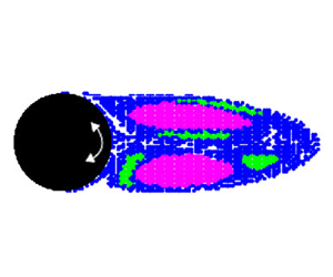
Figure 6. Topological colouring of  $4797$ advected particles at various instants: (a)
  $t=0$; (b)
  $t=0.125 T_p$; (c)
  $t=0.25 T_p$; (d)
  $t=0.375 T_p$; (e)
  $t=0.5 T_p$; (f)
  $t=0.625 T_p$. Each colour corresponds to a different topological class following table 1: class I in green, class II in magenta and class III in blue.
Table 1. Betti numbers  $\beta _k$ (
 $k=0,1,2$), orientability chain
  $\mathrm {o}$ and weak boundary
  $w$ for the cell complexes obtained in the BraMAH analysis of the ROC flow example.

The magenta particles occupy two circular-shaped regions, one per recirculation cell. The green particles define triangular-shaped zones which orbit around the magenta circles. The remaining particles form a ‘background sea’, which is associated with the topological class III. Among the topological classes found for the inspected set of particles in the ROC system, the highest dynamical complexity (associated with the number of holes and the detection of a torsion) corresponds to the background sea of particles.
Finally, a streakline experiment is proposed as an alternative visualization of Lagrangian motion in the ROC case. We use the term ‘separator’ to designate the frontier between differently coloured regions in our topological analysis. We choose the injection points at locations through which the separators do not pass:  $\boldsymbol {p}=(x_1,x_2) / x_1= 0.0525;\ x_2 \in [-0.05:0.005:0.05]$. The streakline patterns at time
  $125 T_p$ are shown in figure 7. The dye distribution confirms that the barriers visualized by the streakline experiment fully coincide with the separators between particle sets belonging to different topological classes. The dye is thus confined in the way revealed by topological colouring.

Figure 7. Streakline experiment for the ROC system with injection points at  $\boldsymbol {p}=(x_1,x_2) / x_1= 0.0525;\ x_2 \in [-0.05:0.005:0.05]$. The picture corresponds to the instant
  $t=125 T_p$ (ROC). The dye (in grey) never invades the circular and triangular regions.
3.2. Driven double gyre
As mentioned before, the ROC moving wall introduces a forcing producing an effect that can be seen as reminiscent of the lateral oscillation of the gyres of the DDG. The DDG equations were introduced by Shadden et al. (Reference Shadden, Lekien and Marsden2005) as a kinematic model for two adjacent oceanic gyres enclosed by land, and acquired a prominent role in the validation of a variety of diagnostics associated with transport and mixing (Shadden et al. Reference Shadden, Lekien and Marsden2005; Allshouse & Peacock Reference Allshouse and Peacock2015a; Balasuriya et al. Reference Balasuriya, Ouellette and Rypina2018). It is known to present chaotic transport between two counter-rotating laterally oscillating vortices (Sulalitha Priyankara, Balasuriya & Bollt Reference Sulalitha Priyankara, Balasuriya and Bollt2017). An analysis of the autonomous writing of the DDG equations for this flow is presented in Charó et al. (Reference Charó, Sciamarella, Mangiarotti, Artana and Letellier2019). This section applies the topological colouring strategy to the Lagrangian motion of particles in this well-studied flow, which is taken as a reference guide for the interpretation of our results.
The DDG equations with the usual parameter settings define the flow in terms of the stream function  $\psi$. The domain under consideration is
  $\varOmega _0=[0, 2]\times [0, 1]$ and parameter values are
  $A=0.1$,
  $\eta =0.1$ and
  $\omega ={\rm \pi} /5$:
 \begin{equation} \psi(x_1,x_2,t)=A\sin({\rm \pi} f(x_1,t))\sin({\rm \pi} x_2), \end{equation}
where
 \begin{gather} f(x,t) = a(t){x_1}^{2} + b(t)x_1, \end{gather}
 \begin{gather} a(t) = \eta \sin\left(\omega t\right),\, b(t) = 1 - 2a(t). \end{gather}
 The time window used for the comparative study of Allshouse & Peacock (Reference Allshouse and Peacock2015a) is the most usual one in Lagrangian diagnosis, and it ranges from  $2.5$ to
  $42.5$. Longer windows have been rarely considered. An example is provided in You & Leung (Reference You and Leung2014) where the time window is
  $320$, eight times longer than the conventional one. In this section, the purpose is to conduct topological colouring choosing a time window such that a comparison is possible with the ROC finite-time analysis. This window is chosen in dimensionless time units, measured with respect to a typical time scale of each flow. Taking the oscillation period of the forcing
  $T_p$ as a reference time scale, an equivalent window for the comparison is
  $T_w=125T_p$. As
  $T_p\ (\textrm {DDG})=10$, this yields a window of
  $1250$, which is four times longer than the one used in You & Leung (Reference You and Leung2014).
The scalar variable that is used for the analysis is the horizontal coordinate of the particle position  $x_1$. The criterion to choose between the two position coordinates does not differ from the one adopted for the ROC analysis. It is here the horizontal and not the vertical coordinate that carries information concerning the gyres. The sampling rate is set to
  $s_r=T_p/100=0.1$. Representative time series are shown for five particles, initially located at
  $P_4=(0.25,0.125)$,
  $P_5=(0.5,0.625)$,
  $P_6=(1,0.5)$,
  $P_7=(0.55,0.5)$ and
  $P_8=(0.4,0.55)$. The FNN and AMI results are shown, together with the time series, in figure 8. As for the ROC case, the embedding dimension is found to be four (
 $m=4$), even if the FNN fraction is already quite low for
  $m=3$. As before, the value that is kept is the highest, in order to simplify the dynamics as little as possible. It is important to remark that
  $m=4$ is compatible with the non-autonomous writing of the DDG equations, presented and analysed in Charó et al. (Reference Charó, Sciamarella, Mangiarotti, Artana and Letellier2019). This work also shows that the observability of the position coordinates, no matter if horizontal or vertical, is equally poor. Dynamical reconstructions from position coordinates in the DDG should therefore not be expected to match the actual phase space of the autonomous version of the DDG system. A poor observability does not prevent BraMAH from being applied, but it precludes the results from being associated in a straightforward manner with the structures in the four-dimensional phase space defined by the autonomized system. The time delay that is adopted is
  $\tau =T_p/5$. Small modifications of the delay parameter around this value do not alter the topological results:
  $m$ and
  $\tau$ are thus kept fixed for the complete set of time series under study.

Figure 8. The DDG system: time series (a–e); FNN (f) and AMI (g) results; embeddings (h–l) for five representative particles initially located at  $P_4=(0.25,0.125)$,
  $P_5=(0.5,0.625)$,
  $P_6=(1,0.5)$,
  $P_7=(0.55,0.5)$ and
  $P_8=(0.4,0.55)$.
Figure 9 shows the cell complexes for each of the five time series, juxtaposed on the three-dimensional projection of the four-dimensional clouds of points. All complexes are of dimension  $2$, as emerges from the BraMAH cell construction process. Homology computations together with orientability chains and weak boundaries allow the distinguishing of five topological classes, whose main features are summarized in table 2. The first three complexes belong to topological classes that were already encountered in the ROC system:
  $\mathbb {K}_4$ corresponds to a strip (class I, green),
  $\mathbb {K}_5$ to a torus (class II, magenta) and
  $\mathbb {K}_6$ is a branched manifold with three
  $1$-holes (class III, blue), with
  $\beta _1=3$ and a torsion that is indicated by the orientability chain. The remaining complexes
  $\mathbb {K}_7$ and
  $\mathbb {K}_8$ have the topologies of a Klein bottle (class IV, red) and of a very particular kind of ‘torus’ involving a torsion and a weak boundary (class V, orange).

Figure 9. Cell complexes juxtaposed on the clouds of points corresponding to the five representative particles in figure 8: (a)  $\mathbb {K}_4$; (b)
  $\mathbb {K}_5$; (c)
  $\mathbb {K}_6$; (d)
  $\mathbb {K}_7$; (e)
  $\mathbb {K}_8$. The
  $1$-holes (generators of
  $H_1$) are highlighted in arbitrary colours. The topological classes associated with each complex are detailed in table 2.
Table 2. Betti numbers  $\beta _k$ (
 $k=0,1,2$), orientability chain
  $\mathrm {o}$ and weak boundary
  $w$ for the cell complexes obtained in the BraMAH analysis of the DDG flow example.

The topologies that emerge in the analysis of a set of  $8528$ particles are of five classes. Results are shown in figure 10 and in supplementary movie 2. The coherent sets may deform in shape as they move, but the frontiers between colours remain considerably well defined. A clear correspondence is found between the identified regions and those observed using a Poincaré section – figure 5 in Charó et al. (Reference Charó, Sciamarella, Mangiarotti, Artana and Letellier2019); or a finite-time Lyapunov exponent study – figure 12 in You & Leung (Reference You and Leung2014).

Figure 10. Topological colouring of  $8528$ advected particles at various instants: (a)
  $t=0$; (b)
  $t=0.1 T_p$; (c)
  $t=0.2 T_p$; (d)
  $t=0.3 T_p$; (e)
  $t=0.4 T_p$; (f)
  $t=0.5 T_p$. Each colour corresponds to a different topological class following table 2: class I in green, class II in magenta, class III in blue, class IV in red and class V in orange.
An additional observation can be made regarding the finite-time nature of the characterization, which depends in principle both on the time window and on the initial conditions. Nonetheless, the topological signatures that we observe are quite robust. In the case of the islands, the family of topological classes that we report for  $T_w=125T_p$ is already reached at
  $50 T_p$. This family remains unchanged for
  $T_w > 50 T_p$. This is not the case for the time series associated with the chaotic sea.
Streakline experiments for the DDG are shown in figure 11. With the injection point situated in the middle of the physical domain  $(1, 0.5)$, the streakline experiment shows that the dye invades the chaotic sea, i.e. the region associated with particles belonging to class III (blue). The non-dyed regions correspond to the islands. Using streaklines to delineate the subzones inside the islands is not possible because there are no suitable injection points satisfying the necessary conditions. For an alternative visualization of the subzones inside the islands, we refer the reader to the stroboscopic sections provided in Appendix D as well as to previously published results using Poincaré sections (Charó et al. Reference Charó, Sciamarella, Mangiarotti, Artana and Letellier2019) and finite-time Lyapunov exponent fields (You & Leung Reference You and Leung2014).

Figure 11. Streakline experiment for the DDG system with an injection point at  $(1, 0.5)$. The picture corresponds to the instant
  $t=125 T_p$ (DDG). The dye (in grey) never invades the circular and triangular regions.
4. Discussion
This section is devoted to a comparison of the topological results for the two examples. Both flows present a particle behaviour that is similar in certain aspects that we will be able to describe precisely using our approach.
Three of the topological classes that are encountered are present in both flows and correspond to groups of particles that behave in an indistinguishable fashion taking into account the selected scalar variable, the time window, the adopted embedding parameters and the studied set of particles. As particles are advected, those tagged with the same colour move together robustly. Two extra classes appear in the DDG: they are associated with subzones in the circular islands. Table 3 summarizes the comparative results.
Table 3. Comparative topological colouring chart for the DDG and the ROC flow examples.

Let us use the already known properties of the DDG system to guide our discussion. The DDG is known to have an embedded horseshoe near the point  $(1,1)$ (Sulalitha Priyankara et al. Reference Sulalitha Priyankara, Balasuriya and Bollt2017), and as a consequence it has fully developed chaos, at least in a restricted subset. This subset can be associated with particles belonging to class III, whose assigned colour is blue. Particles in the chaotic sea of the DDG share their topology with particles in the equivalent ‘background sea’ of the ROC system.
Class III particles have the highest Betti number encountered in this work ( $\beta _1=3$). The three
  $1$-holes and the presence of a torsion are a signature of a higher nonlinearity in the finite-time dynamics of the particles, with respect to the lower-Betti-number and torsionless counterparts. Interestingly enough, recent work (Mangiarotti & Letellier Reference Mangiarotti and Letellier2021) shows that the simplest toroidal chaos is characterized by a three-strip branched manifold with a torsion in one of the strips, motivating further theoretical work on this particular result. It is, however, important to stress that topological features cannot be taken as an indication of chaos; they just provide an indication of the way in which the phase space should be mapped onto itself under the action of the correct model equations under a certain dynamical regime (Sciamarella & Mindlin Reference Sciamarella and Mindlin1999).
We now turn to the topological classes associated with the DDG particles flowing in the islands surrounded by the chaotic sea. These islands can be studied as resonance phenomena in extended phase space (Meiss Reference Meiss1992). From this perspective and providing there are no null points of the flow, particle trajectories in spatially two-dimensional incompressible non-steady flows live either on tori (regular ‘unbroken’ non-resonant trajectories) or on ‘twisted tori’ (regular trajectories within the resonant islands), or appear as trajectories that could fill three-dimensional space between the tori. The manner in which these properties restrict the types of topology that can be observed in finite-time topological analyses using standard delay embeddings is certainly an interesting question, which also deserves further theoretical investigation. As observed by Rypina et al. (Reference Rypina, Pratt, Wang, Özgökmen and Mezic2015), structures that are simple to analyse in a certain space (using, for instance, angle-action variables) become twisted and folded in the space spanned by the position coordinates. This said, it is a fact that structures of classes I, II, IV and V may be seen as deformed tori. Class II is a torus; the strip (class I) is a squashed torus; class IV is a Klein bottle which can be seen as a torus that, in three dimensions, flattens and passes through itself on one side; and class V has already been described as a ‘torus’ with a weak boundary. Flattened tori and strips are indistinguishable by virtue of the cell decomposition process detailed in Appendix B. This is a methodological feature of the BraMAH method which should be taken into account when results are being interpreted. In fact, all the clouds of points analysed with BraMAH in this work lead to the construction of  $h=2$ cell complexes, denoting clouds of points that can be locally approximated with disks of dimension
  $d=2$. Particles in the chaotic sea, which have a higher nonlinearity than those in the islands, are not exempted from this finding. It is important to remark that this is a result and not an assumption of our method. The result is relative to a methodological choice related to the scope of our work, which attempts to distinguish qualitatively different dynamics from a single scalar measured variable and without prior knowledge of the governing equations. The workspace defined by the four-dimensional delay embedding is constructed from a time series of a coordinate of a particle position, without attempting to expand the reconstruction in order to incorporate the forcing dynamics.
Classes IV and V have not been encountered in the ROC system's topological analysis. This translates into an absence of subzones in the circular islands of the cylinder wake. Stroboscopic sections in the Navier–Stokes simulation shown in Appendix D are in agreement with this result, but we cannot be conclusive on the non-existence of subzones for several reasons: firstly, small-scale spatial features may have been smeared out in the numerical simulation due to the finite grid resolution (Fountain et al. Reference Fountain, Khakhar, Mezić and Ottino2000); secondly, the topological study concerns a finite number of particles; and thirdly, the stroboscopic sections are constructed with a finite number of markers.
Finally, and regarding both examples, it is important to stress that the time series associated with the islands have a topology that requires shorter time windows to reach a strong signature than those associated with the background sea. This is in accordance with the quasi-periodic behaviour of particle trajectories in the islands.
5. Conclusions
This paper presents the application of a nonlinear time series analysis technique to the identification of differentiated dynamics from individual fluid particle data, without prior knowledge of the dynamical system or of the nature of its phase space. The results show that, when applied to a set of particles, regardless of their proximity, the approach can be used to unravel the existence, evolution and dynamical nature of coherent sets. The description of the dynamics is not exhaustive and results are relative to a number of methodological choices which include: the specific time window of the analysis, the observable variable used to construct the delay embedding, the parameter settings of the embedding and the set of particles under study. The conclusions reached should not be uprooted from the workspace to which they relate, and in particular, they should not be expected to be analogous to those that would be achieved in an extended phase space. Let us also stress that the number of topological classes encountered for a finite number of particles cannot be taken as encompassing the whole topological diversity of particle behaviour in the flow.
The method requires the choice of an observable that can be input in the form of a scalar time series and provides an output containing the necessary information to reconstruct the (branched) manifold associated with it. In this work, the variable chosen is a coordinate of the particle position. This relates the approach to a series of previously proposed strategies that measure complexity of an individual particle trajectory without involving its nearby neighbours. In this way, a fluid particle can be related to a topology that encodes its finite-time dynamics. The strategy is called ‘topological colouring of fluid particles’ because of the use of colours to label particles according to the topological class that emerges from the analysis. Such a topological class is defined in terms of features of a cell complex that is built from a cloud of points with its delay coordinates determined by a heuristically derived delay and embedding dimension.
The tool can be applied with more than one purpose. It can be used to recognize topologically equivalent particle dynamics in different regions of the same flow, or to relate particle behaviour in a priori unrelated flows, provided the analysis is performed in equivalently scaled time windows. The success of the method is conditioned by the possibility of adequately assessing the topology of the cloud of points obtained after embedding the dataset. If the time series taken as input is excessively noisy, too short in length, very poorly sampled or endowed with a poor observability, the quality of the reconstruction will be weak, producing results that may confound categories which would become distinct with an improved dataset. Methods relying on other Lagrangian descriptors can deal with significantly shorter-length datasets. Another limitation of the method is inherent to the extraction of a continuous representation from a discrete set. Due to this, groups of points that are locally distributed along two preponderant directions will be seen as a locally two-dimensional manifold, even if there are two layers of points which could be seen as enclosing a thin cavity.
The method is illustrated using two cellular flows with particle-trapping regions, with the scope of considering how topological colouring captures the particle dynamics belonging to each coherent set. Although the case studies we discuss are incompressible flows with only two spatial dimensions, the technique is not restricted to them. Our choice is based on the fact that analysis of the results can be quite straightforward. However, the topological approach can, in principle, be applied to more complex cases. The two systems are the wake past a ROC and the analytical DDG. In the first case study, particle trajectories are obtained by numerically integrating the Navier–Stokes equations. The second case study is an analytical system which is probably the most well-studied example in Lagrangian studies. The DDG system cannot be regarded as the approximate solution to a real fluid flow, but it can be seen as a toy model for flows involving a lateral oscillation between two gyres. Although our knowledge of the ROC wake is overwhelming, configurations without vortex shedding at low Reynolds numbers have been relatively left aside.
The examples are first addressed in isolation, to show how topological colouring works in a single flow case. Topological colouring is then conducted on a large particle set, and the results of the analysis strategy are compared against the patterns observed with streakline experiments using appropriate injection points. By advecting the coloured particles, the approach is found to unveil the Lagrangian geography of the flow: the colours in motion define particle sets that move robustly. The frontiers between colours coincide with the borderlines of particle sets that move together, without abandoning the coherent set. Repeated colours, whether in separate regions of the same flow or in independent flow cases, point to a shared dynamics, encoded by the topological features of the cell complexes constructed to approximate the embeddings.
In the comparison between the two examples, topological colouring shows that the numerical solutions of the near field of the ROC flow present coherent sets that have a strong resemblance in shape, motion and topology (dynamics) with the coherent sets of the DDG example within time windows of equivalent length. In this sense, the recirculation cells of the ROC at low Reynolds number can be seen as a ‘materialization’ of a paradigmatic flow model in Lagrangian studies. Both systems, the ROC and the DDG, present a background region with several groups of particles forming islands, which have been studied as resonance phenomena for Hamiltonian systems using a Lagrangian variational formulation. This theory predicts the formation of periodic and quasi-periodic orbits which form a scaffold in the extended phase space and constrain the motion of particles in two-dimensional incompressible flows. The influence of these constraints on the topological classes that can be encountered using delay embeddings is an open question that we hope to address in the future. The prospects of this methodology are multiple and diverse, opening the possibility of addressing Lagrangian studies from an unprecedented perspective.
Supplementary movies
Supplementary movies are available at https://doi.org/10.1017/jfm.2021.561.
Acknowledgements
G.D.C. acknowledges support of her postdoctoral fellowship by CONICET. We would like to thank I.S. Costa and the reviewers for enlightening remarks.
Funding
This work has been supported by the French national programme LEFE (Les Enveloppes Fluides et l'Environnement) and by the CLIMAT-AMSUD 21-CLIMAT-05 project.
Declaration of interests
The authors report no conflict of interest.
Appendix A. Algebraic topology
Algebraic topology is a branch of mathematics that uses algebraic tools to compute topological properties. A basic concept is that of a cell complex  $\mathbb {K}$ (Kinsey Reference Kinsey2012), defined as a finite set of cells of different dimensions such that the interiors of the cells do not intersect. A cell of dimension
  $k$ (
$k$ ( $k \in \mathbb {N}_0$) or
  $k$-cell in a cell complex is a set that can be mapped into the interior of a
  $k$-disk through a continuous invertible map, with boundaries divided into a finite number of lower-dimensional cells, called faces. A cell of dimension
  $k$ is called a
  $k$-cell (
 $k \in \mathbb {N}_0$): a point is a
  $0$-cell, a line segment connecting two points is a
  $1$-cell, a polygon is a
  $2$-cell, etc. Each
  $k$-cell is well defined if it can be mapped through a continuous invertible map into the interior of a
  $k$-disk, and if its boundaries are divided into faces made of lower-dimensional cells. The cell complex has a topological dimension
  $h$ that equals the dimension of its highest-dimensional cells in the complex. Cell complex
  $\mathbb {K}$ is said to be an
  $h$-complex, or equivalently, to have dimension
  $h$. A complex is said to be oriented if each
  $k$-cell with
  $k \ge 1$ is given a direction.
For any given complex, a  $k$-chain is a linear combination of
  $k$-cells with integer coefficients. The algebra of these chains enables a description of the connectivity of the cells at each
  $k$-level in terms of homology groups
  $\mathrm {H}_k$ of a cell complex
  $\mathbb {K}$. Note that computing homology groups from
  $\mathbb {K}$ is a process in which the geometrical information of the coordinates of the
  $0$-cells is not involved. Only the connectivity information, contained in the lists of cells forming the complex, is relevant. With these definitions, a map called boundary operator
  $\partial$ can be constructed which, when applied to a cell of dimension
  $k$, returns its faces of dimension
  $k-1$. The application of the map to a polygon returns its sides, and to a segment returns its end points. The lists of
  $0$-cells forming the cells in the complex are used to construct boundary map matrices whose algebraic handling allows appending in
  $\mathrm {H}_k$ the
  $k$-cycles (closed paths along the complex) that are homologically independent, i.e. that cannot be deformed into each other by a continuous transformation. We denote a homology group in terms of its generators as
  $\mathrm {H}_k = [g_1,\ldots , g_q]$, with
  $q \in \mathbb {N}$. The dimension of
  $\mathrm {H}_k$ is called the
  $k$th Betti number
  $\beta _k$. Let
  $\mathbb {K}$ be a
  $2$-cell complex with homology groups
  $\mathrm {H}_k$,
  $k \le 2$. The
  $k$th Betti will denote (a)
  $\beta _0$: how many connected components (
 $0$-loops) the cell complex is made of; (b)
  $\beta _1$: how many non-equivalent loops (
 $1$-loops) the cell complex sustains; and (c)
  $\beta _2$: how many cavities (
 $2$-loops) the complex encloses.
Homology groups (Betti numbers and generators) provide a topological description of the complex in terms of  $k$-loops, i.e.
  $k$-cycles that do not bound. But in fact, there is more information in the cell complex than that encoded in its homology groups. This extra information may be retrieved by computing the orientability chain
  $\mathrm {o}$. Orienting each highest dimensional cell (each
  $2$-cell for a
  $2$-complex) in the same direction (e.g. counterclockwise), let
  $\mathbb {\gamma }$ denote their sum. The orientability chain is defined as
  $\mathrm {o}= \partial \gamma$ and can be computed along with the homology groups, allowing for the detection of torsions. A weak boundary
  $w$ is defined as a
  $k$-cycle that is not the boundary of any
  $(k + 1)$-chain, but that becomes one if travelled
  $\lambda$ times (Boltcheva et al. Reference Boltcheva, Canino, Aceituno, Léon, De Floriani and Hétroy2011). For instance, the Klein bottle has a torsioned
  $1$-cycle that is not the boundary of any
  $2$-chain, but that becomes one if travelled
  $2$ times, thus defining a weak boundary.
A cell complex is therefore described in greater detail if the generators of the homology groups are provided along with the orientability chain, which may in turn be associated with weak boundaries, in some cases. For instance, the cylinder is a manifold that shares all the Betti numbers with the Moebius strip, but the latter has an orientability chain which is absent in the former. Similarly, the Moebius strip and the Klein bottle are indistinguishable in terms of Betti numbers; both of them have a non-zero orientability chain, but the Klein bottle has a weak boundary that is absent in the Moebius strip. Table 4 lists these topological features for several manifolds.
Table 4. Betti numbers  $\beta _k$ (
 $k=0,1,2$), orientability chain
  $\mathrm {o}$ and weak boundary
  $w$ for some surface manifolds.

Appendix B. The BraMAH method
The BraMAH method computes the topological properties of a cell complex that is built from a cloud of points. In this work, this cloud of points is previously obtained in a dynamical reconstruction from a time series using embeddings. Points obtained in this manner are generally structured so that they lie locally on a  $d$-manifold with
  $d \le m$, with
  $m$ the embedding dimension. This
  $d$-manifold is a topological space with the property that each point has a neighbourhood that is homeomorphic to either a full
  $d$-ball or a half
  $d$-ball (Muldoon et al. Reference Muldoon, MacKay, Huke and Broomhead1993). Such a mathematical object can be used to describe the relative organization of the unstable periodic orbits around which a nonlinear system is structured in phase space. These manifolds can be, for instance, tori or Klein bottles (Mindlin & Solari Reference Mindlin and Solari1997), as well as manifolds with branches. Here, we use the term ‘branched manifold’ for all of them, even when there are zero branches in the manifold.
The algorithm proceeds as in Sciamarella & Mindlin (Reference Sciamarella and Mindlin1999, Reference Sciamarella and Mindlin2001). The first step of this algorithm converts the  $m$-dimensional cloud of points into a cell complex. There are many ways of constructing a cell complex from a cloud of points. Some of them have become very popular with the advent of topological data analysis as a field of research (Zomorodian Reference Zomorodian2010). Our procedure, also used in Charó et al. (Reference Charó, Artana and Sciamarella2020), has the particular feature of building a cell complex such that the
  $0$-cells are a sparse subset of the original cloud of points, and such that each
  $h$-cell represents a group of points that are locally approximating an
  $h$-disk in
  $\mathbb {R}^{m}$. To achieve this, several steps are necessary. A first point
  $\boldsymbol {x_0}=(x_{0,1}, x_{0,2}, \ldots , x_{0,m} )$ is chosen arbitrarily. Let us call ‘patch’ the set of points that lie close to this ‘centre’:
  $\{\boldsymbol {x_i}=(x_{i,1}, x_{i,2}, \ldots , x_{i,m} ), i=1, \ldots ,N_c \}$. In order to determine the size and local dimension of the cell that will be created to approximate this patch, the neighbourhood matrix
  $X \in \mathbb {R}^{n_c \times m}$ is built:
 \begin{equation} X_{i,j}=\frac{1}{\sqrt{n_c}}(x_{i,j}-x_{0,j}). \end{equation}
A local coordinate system centred at  $\boldsymbol {x_0}$ is provided by the singular vectors of
  $X$, with the singular values describing the distribution of the points inside the ball centred at
  $\boldsymbol {x_0}$. For a patch that is approximately lying on a
  $d$-disk in
  $\mathbb {R}^{m}$, the local singular spectrum of
  $X$ has
  $d$ singular values that scale linearly with the number of points in the patch (
 $n_c$) as
  $r$ is increased. This property holds as long as the effects of curvature in the manifold become apparent (Broomhead, Jones & King Reference Broomhead, Jones and King1987; Muldoon et al. Reference Muldoon, MacKay, Huke and Broomhead1993). The remaining
  $(m - d)$ singular values, which measure the deviation from the tangent space, scale as
  $r^{l}$ with
  $l \ge 2$. Using this rule, the
  $d$ singular values and the vectors that span the tangent space approximating the patch under analysis can be identified. The largest possible size of the patch (
 $N_c$) is obtained when the
  $d$ singular values as functions of
  $n_c$ with
  $N_{min}< n_c < N_{max}$ present the best linear regression coefficient. Successive centres are taken so that they are least separated from the previously chosen centre, until every point in the original cloud of points is in at least one patch. Convex hulls are used to transform the patch of points approximating the
  $d$-disk into an
  $h$-cell. By construction,
  $d=h$. The singular vectors are used to orient the cells so that the orientation of each cell is the same as its neighbouring ones. The complex that results from this geometrical procedure is called a BraMAH complex.
The homology groups of the BraMAH complex can now be computed. The labelled list of  $0$-cells is used to build a boundary matrix from which linearly independent rows are extracted. Next, the null spaces of the transpose of the boundary matrix are computed, expressing the
  $k$-borders in terms of the
  $k$-cycles to determine which
  $k$-cycles are homological to others. The
  $k$-cycles that are homologically independent are appended to
  $\mathrm {H}_k$. The integer multiples found in the chain that sums up all the
  $k$-borders of the complex are used to form the orientability chain. The results of this final step of the method are the homology groups of the BraMAH complex expressed in terms of their generators
  $\{\mathrm {H}_k: k=0, \ldots , h\}$, spelled in terms of the
  $0$-cells. The coordinates of the points in the original cloud of points that play the role of
  $0$-cells can be used to plot the cell complex in the reconstructed phase space, as done in figures 5 and 9.
Appendix C. Numerical data validation
Gerris numerical results are validated by plotting the similarity curve of the streamwise velocity ( $u$) along the mid-plane in the recirculation region. The ratio of
  $u/u_{max}$ against the variable
  $({x-R})/{L}$ is plotted in figure 12, where
  $x$ is the streamwise coordinate measured from the cylinder axis,
  $R$ the radius of the cylinder and
  $L$ the length of the closed wake region. Simulation results (continuous line) are juxtaposed with the experimental observations (symbols) reported in Coutanceau & Bouard (Reference Coutanceau and Bouard1977) for a Reynolds number of
  ${Re}=40.5$. An adequate agreement is found between simulation results and experimental data.

Figure 12. Velocity similarity on the rear flow axis in the closed wake. Blue line corresponds to the simulation performed by Gerris and the symbols correspond to a Reynolds number  ${Re}=40.5$ for experimental results found in Coutanceau & Bouard (Reference Coutanceau and Bouard1977).
Since most previous works aim to produce modifications of the vortex shedding phenomena via the rotary oscillations of the cylinder, it is not surprising to find that there are scarce experimental or numerical data for the closed wake regime. Dennis, Nguyen & Kocabiyik (Reference Dennis, Nguyen and Kocabiyik2000) considered a case study in which the flow is at  ${Re}=20$ and the numerical streamlines were compared with the visualizations in Taneda (Reference Taneda1978) for
  ${Re}=40$, when the value of the critical rotation parameter was already overcome. Similarly, our results are compared with Taneda's visualization, but for the same Reynolds number (
 ${Re}=40$). A good agreement is obtained between the streaklines in both cases (figure 13).

Figure 13. (a) Experimental results from Taneda (Reference Taneda1978). (b) Simulation performed with Gerris software.
In order to ensure that the results do not depend on the mesh or size of the selected domain, we perform a convergence analysis considering domains with different number of nodes and width sizes ( $W=10\phi$,
  $W=15\phi$,
  $W=20\phi$,
  $W=25\phi$ and
  $W=30 \phi$), keeping the aspect ratio at
  ${L}/{W}=2$. Figure 14 shows the dynamics of the stagnation point for different cases. Convergence is satisfactorily reached for values of
  $W\geq 25\phi$ and
  $N>39\,000$.

Figure 14. Trajectory of the stagnation point at (a) different width sizes of the domain  $(W)$ (the aspect ratio in all cases is 2) and (b) different number of nodes
  $(N)$.
Appendix D. Stroboscopic sections
The inspection of stroboscopic visualizations is often used as reference for coherent set identification in flows with periodic Eulerian forcing. This appendix presents stroboscopic results for the two examples considered in this work.
For the ROC system, the stroboscopic section is computed for a time window of  $125T_p$ (ROC) (figure 15), with
  $23$ markers placed at the following initial positions:
  $[0.16,0.01];$
  $[0.19,0.015];$
  $[0.22,-0.025];$
  $[0.17,0.04];$
  $[0.18,-0.025];$
  $[0.06,-0.04];$
  $[0.16,0.04];$
  $[0.13,0.005];$
  $[0.06,-0.025];$
  $[0.11,-0.03];$
  $[0.07,0.03];$
  $[0.13,-0.015];$
  $[0.11,0.015];$
  $[0.09,0.03];$
  $[0.08,-0.025];$
  $[0.09,-0.025];$
  $[0.1,-0.035];$
  $[0.08,0.035];[0.09,-0.02];$
  $[0.12,-0.03];$
  $[0.12,0.025];$
  $[0.17,0.025];$
  $[0.13,-0.03]$.

Figure 15. Stroboscopic section obtained for  $23$ initial markers in a time window spanning
  $[0,125T_p$ (ROC)].
For the DDG flow, and over an equivalent length  $125 T_p$ (DDG) (figure 16),
  $14$ initial markers are placed at
  $[1;0.5];$
  $[1;0.9];$
  $[1.25;0.75];$
  $[0.6;0.1];$
  $[1;0.4];$
  $[0.5;0.4];$
  $[0.1;0.85];$
  $[1.1;0.85];$
  $[1.25;0.5];$
  $[1.3;0.8];$
  $[0.25;0.125];$
  $[1.25;0.825];$
  $[1.6;0.875];$
  $[0.4;0.12]$.

Figure 16. Stroboscopic section obtained for  $14$ initial markers in a time window spanning
  $[0,125T_p$ (DDG)].


