


Introduction
Autonomous greenhouses have been developed as a means to grow plants in an optimal environment defined in terms of humidity, temperature, lighting, and gases concentration (Sabri et al., Reference Sabri, Aljunid, Ahmad, Yahya, Kamaruddin and Salim2011; Vera et al., Reference Vera, Osorio-Comparán, Rienzo, Duarte-Mermoud and Lefranc2017). Such technology has many advantages such as a better management of resources and an off-season growth of high-quality crops (Rabago et al., Reference Rabago, de Santago and Moncada2013; Abas and Dahlui, Reference Abas and Dahlui2015). However, the design of such a greenhouse is not an easy task. One major issue is its layout design. In general, the layout design is the spatial management of different elements in a given space based on domain-specific objectives. In architecture and urban design, the ease of access from rooms to hallways could be a domain-specific objective (Koenig and Schneider, Reference Koenig and Schneider2012). Another example closer to the design of a greenhouse is the design of a satellite where the domain-specific objective is to ensure that every element can carry out their functions (Taura and Nagasaka, Reference Taura and Nagasaka1999). Furthermore, layout and domain-specific objectives are usually conflictual. Indeed, the layout design of an autonomous greenhouse needs to manage two important conflictual objectives, which are to maximize the size of the pack soil and to minimize the amount of resources needed. On top of those objectives, the greenhouse must be functional and must allow an optimal environment for the growth of specific plants. Since an autonomous greenhouse is a mechatronic system, it is essential to consider interactions among the components during the design phase (Mohebbi et al., Reference Mohebbi, Baron, Achiche and Birglen2014; Torry-Smith et al., Reference Torry-Smith, Mortensen and Achiche2014) to increase its efficiency. To overcome this challenge, the layout design of a greenhouse consists of concurrently solving three main issues.
The first issue is to define the size and location of the pack soil as well as the storage of resources (e.g. water tank). The size of both the pack soil and storage of resources is defined by the plants chosen to be grown in the greenhouse. Indeed, plant seeds need a space between each other to properly grow, which means that the size of the pack soil depends on the number of seeds. As for the storage of resources, each individual plant needs to consume a certain amount to properly grow as well. This means that a prior knowledge about the ideal environment of the chosen plant is needed.
Since the greenhouse has to be autonomous, a set of sensors to acquire data of the current environment is required. Hence, the second issue is the need to define the size and performance of sensors (e.g. humidity) and actuators (e.g. water pump) which control the greenhouse environment. A set of actuators must be present to modify the environment. Depending on the model of sensors and actuators, the size and the performance of the system can change in terms of the volume allocated for both the plant growth and the assessment of the environment.
As for the locations of these components, they depend on the third and last main issue, which is the interaction between all the greenhouse components. Indeed, the sensors, actuators, pack soil, and storage of resources must be carefully positioned to avoid the malfunction of the greenhouse. A malfunction can occur when one component has adverse/negative effects on other components as reported by Chouinard et al. (Reference Chouinard, Achiche, Leblond-Ménard and Baron2017, Reference Chouinard, Achiche and Baron2019). For example, the temperature sensor cannot be placed close to the heater to avoid an erroneous reading of the temperature, which could lead to freezing, or drying the pack soil. It is worth mentioning that in this paper, we will consider the same categories in terms of heat, electromagnetic effects (EMFs), and vibrations when present.
The main contribution of this paper is the development of a methodology to formulate an optimization problem for the automated layout design of a greenhouse considering the three issues mentioned above in terms of (1) size and location of pack soil and storage of resources, (2) size and performance of sensors and actuators, and (3) location of components considering their adverse effects.
First, the problem statement of the layout design of a greenhouse is carried out and translated into an optimization problem. Using evolutionary computing [a genetic algorithm (GA)], the size, location, and parameters of every component of the greenhouse are optimized.
Background and literature review
We focus on studies of autonomous greenhouse design and greenhouse layout design. The research trends concerning autonomous greenhouses are generally targeting climate control, wireless networks, and integrated design.
Autonomous greenhouse
This part of the literature review is carried out to identify the product specifications needed to design an autonomous greenhouse. It is destined to systematically formulate the problem statement presented in the next section.
Researchers are interested in improving the assessment of the environment of a greenhouse in different situations. Castañeda-Miranda and Castaño (Reference Castañeda-Miranda and Castaño2017) made a comparison between an autoregressive algorithm (ARX) and an artificial neural network to predict the internal temperature of a greenhouse based on both external and internal parameters, such as the outside temperature and the humidity. This study found that the artificial neural network provides a better prediction than ARX. The method is tested with data from a greenhouse and a weather station. Romantchik et al. (Reference Romantchik, Ríos, Sánchez, López and Sánchez2017) designed a cooling control system to prevent the temperature of the greenhouse of exceeding 25°C using fan-pad systems. Based on a ventilation system, an algorithm is developed to support the design of a photovoltaic solution, which would supply the necessary energy. Vera et al. (Reference Vera, Osorio-Comparán, Rienzo, Duarte-Mermoud and Lefranc2017) built a greenhouse with its environment controlled by monitoring the temperature, humidity, carbon dioxide, and illumination levels. In this greenhouse, a heat sensor and a heater controlled the temperature. A humidity sensor for soil controlled the humidity of the soil and a solenoid valve fed the water. A relative humidity sensor and a micro-sprayer controlled the humidity of the air. A carbon dioxide sensor and a fan regulated carbon dioxide levels. Finally, a combination of a luminosity sensor, luminosity source, and a timer controlled the illumination. In their research works, Abas et al. (Reference Abas and Dahlui2015, Reference Abas, Salman, Ridwan and Adzhar2016) used the temperature, humidity, and irradiance acquired by sensors to control the temperature, the humidity, and the interval of time between the activation of an irrigation system. An intruder detector activates the intruder repellent using electric fences and ultrasonic sound. The whole system is powered by a solar panel. Matos et al. (Reference Matos, Gonçalves and Torres2015) automated a fodder production part of a hydroponic system (growing plants without soil). The system automatically placed seeds in the trays, and managed the nutrient solution preparation and the water distribution. Paraforos and Griepentrog (Reference Paraforos and Griepentrog2013) used a multivariable control of a greenhouse in terms of carbon dioxide quantity, temperature, and humidity. A nonlinear steady-state model is used to develop an input/output linear decoupled controller by linearizing and discretizing the model for given operation points. Pala et al. (Reference Pala, Mizenko, Mach and Reed2014) proposed a control strategy for an aeroponic system. In their work, first, a network of sensors and actuators is implemented to monitor the environment through a user interface to relay the information to the user and to allow the user to manually control the system if needed. Second, the aeroponics system design called Aero Pot is presented. The Aero Pot is a nutrient distribution system composed of two nozzles, where the nutrients are given to a plant and a motor to move the nozzle from one plant to another. The optimization of the system is done using a GA. The user can define the number of lights and pumps and their power consumption. The GA first optimizes the power consumption, then provides the power schedule of components for 1 day. The preliminary results of this optimization are promising since the first experiments demonstrated that with a reasonable power consumption, the plant was healthy. Rabago et al. (Reference Rabago, de Santago and Moncada2013) designed a solar-powered automatic greenhouse. The system controlled the moisture, the temperature, and the irrigation schedule using information about the humidity, the moisture, the temperature, and the soil mixture. The components were solar panels, batteries, valves, a relative humidity sensor for the air, a humidity sensor for the soil, a halogen lamp to heat, fans, and microcontrollers. In the work presented by Hahn (Reference Hahn2011), a fuzzy controller is developed to prevent tomatoes from cracking because of the overheating. To control the temperature of the crop, a shading screen control and an irrigation system control are used. The solar radiation, the substrate temperature, and the canopy temperature were the inputs of the fuzzy controller, while the output was the command sent to the irrigation system and the motor controlling the shading screen position. Schubert et al. (Reference Schubert, Quantius, Hauslage, Glasgow, Schroder and Dorn2011) proposed a greenhouse module design for extraterrestrial habitats. The system design started by suggesting multiple designs of the greenhouse module, which contained the growth system. The growth system is composed of the germination unit which starts the growth of the plants before transferring them in a grow pallet. The growth pallet is then placed in a growth channel, where the environment is controlled to satisfy the needs of a given plant for every stage of its growth. The growth channel unit is filled with multiple growth channels installed on a conveyor system. Finally, the greenhouse module is integrated with eight subsystems to control the environment of the plants. Xu and Li (Reference Xu and Li2008) developed a greenhouse control system using multiple agents. The intelligent control center is composed of a collecting artificial agent to gather data from the greenhouse, which is processed by the data processing one. The data transmitting agent then stores the information in a database. The intelligent control center also has an agent, which controls the greenhouse environment in terms of temperature, illumination, humidity, and carbon dioxide concentration. Herrero et al. (Reference Herrero, Blasco, Martínez, Ramos and Sanchis2007) implemented an elitist multiobjective evolutionary algorithm to identify the parameters of a greenhouse model. The greenhouse model used is composed of 15 parameters to estimate the internal temperature and humidity. Using the implemented evolutionary algorithm and a set of data obtained from an operating greenhouse, a Pareto-optimal set of the greenhouse model was found. Then, the greenhouse model from the set of criteria closer to the ideal optimality criteria was validated using another set of data obtained from the same operating greenhouse.
Most of the time, researchers use wireless communication networks of components to monitor and control the climate of the greenhouse. Hence, the use of wireless communication adds complexity in the design of autonomous greenhouses. In Azaza et al. (Reference Azaza, Tanougast, Fabrizio and Mami2016), a fuzzy logic-based controller combined with a wireless communication system based on the ZigBee platform controlled the climate of a greenhouse. The temperature, humidity, carbon dioxide, and illumination integrated a fuzzy set beside the external meteorological variables and the set points given by a user. Then, a decision scheme, which represented the observer design flow, was set up in terms of ventilation, heating, humidification, and dehumidification. Finally, the fuzzy logic controller is implemented using FPGA programming to assess the greenhouse environment in terms of temperature and humidity using the heating and ventilating system. In Krishna et al. (Reference Krishna, Madhuri and Anuradha2016), a wireless network based on ZigBee assessed the greenhouse environment in terms of humidity, moisture, and temperature. The sensors sent the data to an ARM7 microcontroller, which is used as a ZigBee transmitter. The data are then sent in real time to a central unit combined with a Zigbee transmitter in order to monitor the data. Goumopoulos (Reference Goumopoulos and Mukhopadhyay2012) and Goumopoulos et al. (Reference Goumopoulos, O'Flynn and Kameas2014) developed an automatic irrigation control system using machine learning and wireless sensor network (WSN) information formed of multiple nodes, where one node monitored a zone containing multiple plants. The control strategy had three main components. First, the ontology of the plant is used to define the rules for the decision-making based on prior knowledge. Second, the decision support system acquired all the information from the data analysis of the greenhouse in order to make a decision for the well-being of the plant. Finally, the machine learning is used to obtain new connections among the data acquired. Three types of sensors are used: soil moisture sensors, humidity sensors, and thermistors for air temperature. In Sabri et al. (Reference Sabri, Aljunid, Ahmad, Yahya, Kamaruddin and Salim2011), a fuzzy logic approach and a wireless network based on ZigBee controlled the greenhouse. The differences in temperature and humidity of the greenhouse are monitored and used as inputs for the fuzzy controller. The fan, heater, and humidifier command are the output of the controller. Ferentinos et al. (Reference Ferentinos, Katsoulas, Tzounis, Bartzanas and Kittas2017) made a sensitivity analysis of a WSN reading in function of the solar exposition level. They made experiments to evaluate which readings were more stable between three expositions level. The first exposition level was labeled as “exposed nodes” and was a WSN directly exposed to solar radiation. The second one was labeled as “boxed nodes” and was fully protected from solar radiation by a ventilated box. The last one was labeled as “shaded nodes” and used a metallic surface to protect the nodes from direct sunlight. The analysis showed that the most stable reading was from the “shaded nodes”. Hence, they used “shaded nodes” in a commercial cucumber greenhouse. Using this system, they studied plant conditions such as the transpiration of the crops and the leaf temperatures.
The climate control of a greenhouse adapted and integrated to infrastructure or uncommon environments is also an area of research. Nadal et al. (Reference Nadal, Llorach-Massana, Cuerva, López-Capel, Montero, Josa, Rieradevall and Royapoor2017) proposed an integrated rooftop greenhouse (iRTG) at the Autonomous University of Barcelona campus. To grow crops successfully, the iRTG recycled many resources from the building to control airflow and temperatures of a greenhouse. Indeed, the whole building adopted a mode of operation depending on the season to control the ventilation system of the building. For example, when the temperature was too high, the windows are open to cool down the greenhouse. With the iRTG, tomatoes and lettuce crops are produced. Poulet and Doule (Reference Poulet and Doule2014) made a preliminary design of a greenhouse for food and for a Zen garden (for crew emotional state) called GreenHab. The GreenHab purpose is to eventually be used as a greenhouse on Mars. At the moment, the growth of different lettuces in GreenHab is being studied and tested at the Mars Desert Research Station of the Mars Society of Utah. The study of GreenHab is carried out in terms of temperature, illumination, and humidity. The system is only partially automated since the crew can also modify the environment of the greenhouse. Giroux et al. (Reference Giroux, Berinstain, Braham, Graham, Bamsey, Boyd, Silver, Lussier-Desbiens, Lee, Boucher, Cowing and Dixon2006) designed a greenhouse for Mars's environment. The greenhouse is equipped with sensors to monitor the humidity, temperature, and radiation. The actuators used were the heaters, the fan, and the exhaust fan, which are controlled based on the temperature of the greenhouse environment. The greenhouse can operate all year long by changing its operation mode based on the external environment, such as the outdoor temperature. Furthermore, the water distribution is done manually. An analysis of a greenhouse environment and power consumption over a year is also carried out.
From this literature review, one can conclude that the main function of an autonomous greenhouse is to ensure the growth of plants by controlling the climate of the greenhouse. Based on this main function, a list of product specifications will be listed in the next section for the layout design of an autonomous greenhouse.
Greenhouse layout design
Komasilovs et al. (Reference Komasilovs, Stalidzans, Osadcuks and Mednis2013) used a GA called GAMBot-Eva to optimize the design of a robotic system traveling through the greenhouse layout, evaluating health conditions of plants, and spraying pesticides on them if needed. The optimization problem took into account tasks of the robot, the price, and the energy consumption of the robot components. However, the greenhouse layout is fixed, and the optimization is done with parameters of the robotic system. Eben-Chaime et al. (Reference Eben-Chaime, Bechar and Baron2011) optimized the overall cost of a greenhouse layout based on different expenses, such as seedlings and labor costs, for different greenhouse layouts. The layout can be changed in many ways to reduce the overall cost of the greenhouse. Four different layouts are presented, and the overall cost is calculated. Hence, the performance of the greenhouse is not taken into account to choose the layout. Ferentinos et al. (Reference Ferentinos and Albright2005) and Ferentinos and Tsiligiridis (Reference Ferentinos and Tsiligiridis2007) optimized the topology of the WSN for precise agriculture applications in terms of energy consumption and sensor sensitivity characteristics. The problem is also subjected to connectivity and spatial density constraints. This multiobjective optimization is turned into a single-objective optimization using a weighted sum approach. The optimization problem is solved with a GA using binary representation. A dynamic optimal design algorithm is also included in the GA for sensors with battery capacities. Ferentinos and Albright (Reference Ferentinos and Albright2005) also used a GA using binary representation for the placement of the lighting system for a greenhouse. The optimization considered a different lighting characteristic, such as the light uniformity, as well as economical aspects, such as the investment costs. They also used a penalization function in order to avoid shading effects that can happen when designing a lighting system. The problem is rewritten as a single-objective optimization problem using a weighted sum approach.
Main objective and contributions
Our previous section shows that, until now, there are only a few works covering the greenhouse layout design. Moreover, these works do not fully consider the layout in the design of the autonomous greenhouse. This might be caused by an incomplete problem statement of the layout design. Hence, the problem statement of the layout design needs to be improved to rigorously define the components needed and their interaction.
To the best of our knowledge, the evolutionary layout design of greenhouses considering the placement of components and their interaction (dependencies) has never been done. The main contribution of this paper is a novel methodology to formulate a more comprehensive problem statement for layout design as shown in Figure 1. Furthermore, the methodology also considers the translation of a problem statement from an engineering design perspective to the formulation of an optimization problem. First, a problem statement is developed by identifying the components of an autonomous greenhouse and their interactions. The problem statement is then translated into an optimization problem which is solved using a GA.

Fig. 1. Highlights of contributions in the general methodology.
The rest of the paper will be structured as follows: “Problem statement” defines the problem statement of the layout design of a greenhouse. “GA implementation” reviews similar problems solved using algorithmic approaches and describe the implementation of the GA. “Results and discussion” report the results and analysis of the design of an autonomous greenhouse obtained by the GA used in this paper. Based on these results, the main limitations and future research avenues are identified. Finally, “Conclusion” concludes on this paper.
Problem statement
Identification of autonomous greenhouse components and interactions
Using the six product-related dependencies presented by Torry-Smith et al. (Reference Torry-Smith, Mortensen and Achiche2014), we identify the components needed for the development of an autonomous greenhouse. The product-related dependencies are defined in terms of function (Fu), property (Pr), and mean (M) of the product and their interactions. The function is defined as the tasks that systems and/or subsystems must be able to complete. Here, property refers to a property of the system such as the mass. Often, the property is affected by the choice of means. Finally, the mean is what is used to accomplish a function. The approach developed here is framed by the product-related dependencies methodology which offers a general framework that is generally used in multidomain system design. This can be easily generalized to other complex system design activities, such as for mechatronics, where designers can have a more thought out starting point early in the design process.
Fu–M can be explained by the following: a function is realized by a mean, which can be further decomposed into subfunctions and so on. Using this definition, some components can be identified:
1) Fu–M disposition and cumulative Fu–M: Figure 2 presents the results of the Fu–M decomposition to identify the components.
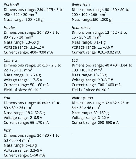
2) Adverse effect: As mentioned above, the adverse effects considered in this paper are categorized in terms of heat, vibration, and EMFs. We also add another category which is the obstruction of a component field of view. This will be represented by OBS in Table 1. Although, it is difficult to evaluate this fourth category considering that the dimensions of each component are still unknown, it is possible to estimate an order of magnitude for each of the component. For example, generally a water tank is bigger than a heat sensor; hence, the water tank has more chance to obstruct the field of view of a component such as a camera. A table such as Table 1 is used by Chouinard et al. (Reference Chouinard, Achiche, Leblond-Ménard and Baron2017, Reference Chouinard, Achiche and Baron2019) to identify components generating adverse effect and those who are affected by these adverse effects. The first column is the list of components. The second column is a qualitative evaluation of the intensity of adverse effects generated by the component. The last column is a qualitative evaluation of the negative impact of the component affected by adverse effects.

Fig. 2. Organigram representing the Fu–M decomposition.
Table 1. Relation between components and adverse effects

Considering Table 1, it is possible to identify the most detrimental combinations of components and to formulate the following guidelines to avoid these adverse effects:
i. Heater cannot be close to heat sensor.
ii. LED cannot be close to heat sensor.
iii. The components cannot prevent the LED from lighting the pack soil.
iv. The components cannot prevent the camera from filming the pack soil.
Pr–M can be explained by the following: a property is affected by the chosen means. Using this definition, the rest of the components can be identified:
Property scheme:
Property 1: Mass of the system. The mass is calculated by making the sum of all the mass of the means. For autonomous greenhouse, a low mass can be an indicator of low consumption of resources and is generally favorable.
Property 2: Electrical current of the system. We approximate the electrical current by summing all the electrical current of the means. Generally, a low electrical current consumption is also favorable.
Property 3: Electrical voltage of the system. The mean with the highest voltage will be the reference point of this property. Generally, a low electrical voltage is favorable.
M–M can be explained as a dependency between two means:
1) Volume allocation:
i. The space between the LED and the pack soil is the volume allocated to the plant since plants grow toward the light.
ii. Enough space must be allocated to store water and the amount of water depends on the plant.
iii. The camera must be able to film the pack soil as much as possible.
2) Physical interface:
i. The water tank, water pump, and pack soil must be linked by pipes to ensure the water distribution system.
ii. The LED must light as much as possible the pack soil.
iii. The fan must be close to the heater for better heat convection.
It is possible to see that by identifying the Fu–M disposition and cumulative Fu–M, the list of components needed to synthesize an autonomous greenhouse is found:
C1.Heater: to heat the greenhouse.
C2.Water tank: to contain the water for the plants.
C3.Pack soil: to contain the seeds of the plant.
C4.Heat sensor: to acquire temperature data from the environment.
C5.Camera: to follow the growth of the plants.
C6.Fan: to ensure air circulation in order to stabilize the room temperature.
C7.LED: to provide the light necessary for photosynthesis.
C8.Water pump: to allow water distribution from the water tank to the pack soil.
C9.PCB: to monitor pressure, humidity, O2, and CO2 (sensors).
C10.Pipes: to link the water tank, the water pump, and the pack soil for water distribution.
Furthermore, the adverse effects as well as the Pr–M and M–M dependencies give guidelines to handle the placement of components within the system. To assign the strength of a dependency, the design structure matrices (DSMs) (Pimmler and Eppinger, Reference Pimmler and Eppinger1994; Browning, Reference Browning2016) is used in this work. DSMs have been used for modeling interactions between components and/or subsystems in many fields such as mechatronic design. The DSM representation and the scale value represented by Pimmler and Eppinger (Reference Pimmler and Eppinger1994) are adapted to model the layout component interactions. In this work, a layout component interaction is composed of three characteristics: closeness, field of view (FOV), and physical connection. These three matrices can model the layout design of most complex systems including mechatronic systems.
1) Closeness of two components: In this matrix, each value follows the scale shown in Table 2 to evaluate the closeness of two components.
Table 2. Closeness strength scale

And so, closeness matrix for the first nine components mentioned above (the pipes are excluded from the DSMs) is:

The selection of weights for the closeness matrix is justified as follows: the assigning of the weight is based on the interaction of the components and the impact on the main function requirement which is to ensure the growth of the plant. Hence, the most detrimental interaction is related to the temperature regulation. The heat sensor (C4) absolutely needs to be as far as possible from any heat sources. In our case, the heater (C1) and the LED (C7) are the main heat sources. Therefore, the (C1, C4) and (C7, C4) cells have the value −2. Still considering the temperature aspect of the greenhouse, the environment temperature must be uniform. A local hot spot or cool spot on the pack soil could prevent the growth of plants. For this reason, the heater (C1) and the fan (C6) need to be as close as possible in order to assure a proper heat flow. This explains why the value of (C1, C6) cell is 2. Finally, the water distribution is composed of a water pump (C8), a water tank (C2), and the pack soil (C3) which are connected by the tubes. The length of the tube could be reduced if all the three components are closed to one another. There are advantages coming along with the reduction of tubes such as decreasing the active time of the pump which leads to a decrease of energy consumption. Hence, the (C2, C3), (C2, C8), and (C3, C8) cells have the value of 1.
2) Interaction between the FOV of two components: In this matrix, each value follows the scale shown in Table 3 to estimate the importance of the interaction between the two components FOV.
Table 3. Field of view strength scale

And so, the FOV matrix is given by:

This matrix refers to two components which are the LED (C7) and the camera (C5) which need to illuminate and capture the pack soil (C3), respectively. The values of cells (C3, C5) and (C3, C7) are 2 because the fulfilment of their functional requirements is more sensitive to the relative position of the pack soil. Indeed, the LED must uniformly illuminate the pack soil as much as it can to allow every seed a chance to grow. As for the camera, it must capture most of the pack soil to help the operator identify a malfunction or to visually assess the health of the plants.
-
3) Physical connection of two components: In this matrix, each value indicates the number of links (wire and/or pipe) that two components need. And so, the physical connection matrix is:

Formulation of the optimization problem
Based on the problem statement for the synthesis of an autonomous greenhouse mentioned in the last section. The translation of the problem statement to an optimization problem will be done in this section.
First, two types of objectives included in the overall objective of the solution are developed. The first type is the component-specific objectives (CSOs). CSOs concern only the design of the component itself. The second type is the layout design objectives (LDOs). LDOs cover the layout design based on the placement of components of the greenhouse.
The CSOs are:
1. Minimizing the volume (except for the pack soil and water tank volume, which need to be maximized)
2. Minimizing the mass.
3. Minimizing the energy consumption.
The LDOs are:
1. Minimize the distances between the pack soil, the water tank, and the water pump.
2. Minimize the distance between the heater and the fan.
3. Minimize the distance between connection points linking two components.
4. Maximize the distance between the LED and the heat sensor.
5. Maximize the distance between the heater and the heat sensor.
6. Maximize the lighting of the pack soil by the LED.
7. Maximize the view of the pack soil captured by the camera.
For LDOs, a weight is assigned to every one of them based on the DSMs mentioned before. Moreover, all distances and lengths use the 3D Euclidean distance. As for the sixth and seventh LDOs, the objectives use the 3D Euclidean distance between the line of sight (LOS) of two components as shown in Figure 3. The ideal LOS for the second component (C2) is the desired LOS presented in Figure 3. Hence, the distance between the desired LOS and C2 needs to be minimized.

Fig. 3. Objective based on the LOS of components.
Second, the design of an autonomous greenhouse is necessarily subjected to a set of constraints coming from multiple sources. All of these constraints need to be respected in order to obtain a feasible solution. In this work, we consider three sources of constraints. The first source of constraints is based on the limited space allowed and the physical boundary of every component. The second source originates from the interaction of the components. The third and last source is the specifications of the greenhouse which would be given by a customer. In this work, the following constraints are considered:
1. The overall volume occupied by the components must be lower than the greenhouse volume.
2. The boundaries of a component must fit within the boundaries of the greenhouse.
3. The boundaries of a component cannot overlap another component's boundaries.
4. The FOV of the camera must be wide enough to capture the pack soil.
5. The FOV of the LED must be wide enough to light the pack soil.
6. The overall mass must be lower than a defined mass.
7. The overall energy consumption must be lower than a defined quantity of energy.
8. The voltage and current of each component cannot exceed given thresholds.
The first three constraints come from the limited volume allowed. The fourth and fifth constraints are related to the interaction between components. The last three constraints are the product specifications which stem from customers’ needs.
Finally, the optimization problem can be summarized as a single-objective optimization problem
 $$\left\{{\matrix{ {{\rm Minimize}\mathop \sum \limits_{i = 1}^n w_iO{\lpar {\vec{x}} \rpar }_i} \hfill \cr {{\rm subjected\;to}} \hfill \cr { {\rm CT}_j\;{\rm for}\;j = 1\comma \;\ldots \comma \;m}. \hfill \cr } } \right.$$
where  $\vec{x}\;$is the decision variable vector. It contains the parameters of every component as shown in Figure 4, O (
 $\vec{x}_i\rpar$ is the ith objective of all the objectives (CSOs + LDOs), wi is the weight associated with the ith objectives of all the objectives, and CTj is the jth constraints.

Fig. 4. Decision variable vector: vector representation of components within a solution and the parameters within a component.
The weight is 1 for all CSOs because they need to be optimized in order to overcome the constraints and to respect the product specification, but they are not the most important aspect of the optimization to accomplish the main function which is ensuring the growth of the plant. For LDOs, the weight can be found in the DSMs. For our formulation, n is the total number of objectives and m is the total number of constraints. In this work, n is equal to 10 and m is equal to 8.
GA implementation
Considering the optimization problem given in “Problem Statement”, the design of an autonomous greenhouse can be seen as a many-objective optimization problem (MaOP) like most real-life applications in engineering (Fleming et al., Reference Fleming, Purshouse and Lygoe2005). Even though algorithms have been developed since 2003 (Hisao et al., Reference Hisao, Noritaka and Yusuke2008; Li et al., Reference Li, Li, Tang and Yao2015; Huang et al., Reference Huang, Zhang and Li2019) to solve MaOPs, we will use a single-objective optimization to solve the layout design of an autonomous greenhouse for two main reasons. First, we are not searching for a Pareto front of design. The main objective of this research is to thoroughly express a problem statement and its optimization formulation for autonomous greenhouse. Hence, we attempt to find one near-optimal design to validate the formulations based on the a priori preferences of the designers. Second, selecting an adequate algorithm for a given problem is not a trivial task as shown by the comparative study of Panerati and Beltrame (Reference Panerati and Beltrame2014). The study consists of evaluating the performance of 15 multi-objective design-space exploration algorithms on the optimization of three real-life applications using three performance metrics such as the average distance from the reference set. The comparison showed that no algorithm outperforms the others; however, general guidelines on the simulation time and size of the design space were found. Another example (Saldanha et al., Reference Saldanha, Soares, Machado-Coelho, dos Santos and Ekel2017) defines the best algorithm between non-dominated sorting GA-II, predator–prey, and multiobjective particle swarm optimization (PSO). To achieve this, they needed to evaluate the results of each algorithm with performance metrics and a decision-making method called PROMETHEE. They found that the multiobjective PSO was the best algorithm in order to design a shell-and-tube heat exchanger because of its robustness. Furthermore, the no-free lunch theorem (Wolpert and Macready, Reference Wolpert and Macready1997) inform us that a priori no algorithm outperforms another one in all optimization problems. Consequently, selecting an inadequate algorithm could output a poor set of Pareto front solutions which could erroneously lead us to believe that the formulation is inadequate. Hence, we decide to aggregate all the objectives using scalarizing functions (Marler and Arora, Reference Marler and Arora2004; Kaim et al., Reference Kaim, Cord and Volk2018) into a single-objective optimization. Scalarizing functions can be used to articulate the preferences of the designers in order to find one solution from the Pareto front. Using this, we will better assess if our formulation is able to find a feasible and near-optimal solution.
Evolutionary algorithms are also known to be effective when it comes to solving single-objective combinatorial optimization problems as explained in surveys concerning facility layout problems (Drira et al., Reference Drira, Pierreval and Hajri-Gabouj2007; Moslemipour et al., Reference Moslemipour, Lee and Rilling2012; Ahmadi et al., Reference Ahmadi, Pishvaee and Akbari Jokar2017). Other domains also use evolutionary algorithms. Yu et al. (Reference Yu, Yang and Cheng2007) used a parallel genetic implementation to optimize shopping routes of shoppers in terms of the shortest car-based route. The parallel genetic implementation is used to reduce the computational time by dividing the resources of the computer to execute the GA operators. The implementation is tested on a case study in Dalian City, China. Zhao et al. (Reference Zhao, Hsu, Chang and Li2016) implemented a GA to minimize the mental workload of human operators in the mixed-model assembly line based on many factors such as the assembly complexity and operator experience. The motivation of this work is to reduce the errors resulting from human mental fatigue and to improve the efficiency of the assembly line. Ribas et al. (Reference Ribas, Yamamoto, Polli, Arruda and Neves2013) combined hybrid micro-GA and mixed integer linear programming to schedule and plan an oil pipeline network. The scheduling considered the management of the production and the operation, the inventory management, and the transportation of oil to name a few. The use of micro-GAs was to lower the computational time and resources while keeping good solutions. The developed algorithm is tested on Brazilian pipeline networks. Zhang and Zhang (Reference Zhang and Zhang2007) developed a GA to design a network based on the network partition problem. This optimization problem goal was to reduce the inter-network communication while managing the traffic distribution over subnetworks. The implemented GA considered the traffic matrix, the devices needed in a network as well as the current devices used in the industry. To validate the effectiveness of the GA, a simulation is carried out. Király and Abonyi (Reference Király and Abonyi2015) made a GA implementation to solve a multi-traveling salesmen problem (mTSP). This work was greatly inspired by an industrial case study, where an electric and gas energy supplier needed to transfer materials from different sources to a specific location. This issue is an mTSP, which is a combinatorial optimization problem. Cheng et al. (Reference Cheng, Gupta, Ong and Ni2017) combined PSO with a multitasking coevolution mechanism. The novelty resides in the multitasking coevolution mechanism, where two or more tasks have their own objective functions to optimize for an overall problem. The tasks were usually influencing each other, which led to a concurrent optimization problem. To validate the developed algorithm, the optimization of the productivity of a composite manufacturing is simulated. The two tasks to be optimized were the resin transfer molding and the injection/compression-liquid composite molding because these processes shared a part of the design space. Saleh and Chelouah (Reference Saleh and Chelouah2004) used an algorithm based on the GA to locate the position of an unknown point on Earth using the satellite equipment. Such problems are called a GPS surveying network, which is a variation of the problem from the classical survey network problem. The goal is to optimize the robustness of a GPS network based on the resources available to the network (e.g. cost, personnel, and satellite). Guzmán-Cruz et al. (Reference Guzmán-Cruz, Castañeda-Miranda, García-Escalante, López-Cruz, Lara-Herrera and de la Rosa2009) compared five optimization algorithms in order to define which algorithm is better for the calibration of a specific greenhouse model. The five algorithms are GAs, evolutionary programming, evolutionary programming, least squares, and sequential quadratic programming. The greenhouse model is composed of 16 parameters and is used to estimate the internal humidity and temperature. For the calibration of the greenhouse model, the evolutionary programming was the best choice. Elferchichi et al. (Reference Elferchichi, Gharsallah, Nouiri, Lebdi and Lamaddalena2009) used a weighted sum GA to define the optimal inflow hydrograph to provide water to different farmers without emptying the reservoirs available. The objective function as well as the constraints were formulated using the water level of every reservoir. The weight associated with an objective function was defined with a sensitivity analysis. Based on the on-demand water quantity of the farmers, the GA was able to find an inflow hydrograph to supply the farmers without emptying the reservoirs for a specific period of time. Ushada and Murase (Reference Ushada and Murase2009) made the design of a customizable greening material combining three main tools. The first tool was the swarm modeling to set the design attributes. Then, the second tool was the desirability model to define the importance of design attributes based on the consumer mentality constraints. Finally, the third tool was the PSO to optimize the design of a greening material. The developed methodology was tested in a case study designing Sungoke moss. Utamina et al. (Reference Utamima, Reiners and Ansaripoor2019) developed a novel evolutionary algorithm called evolutionary hybrid neighborhood search (EHNS) which combine mutation-based neighborhood search and Tabu search algorithms. The first step of the EHNS loop was the mutation-based neighborhood search algorithm which uses the roulette wheel selection to pick individuals within the population. Then, mutation operators were applied to the chosen individuals. The second step was the replacement of the current individuals by the mutated individuals. If the best new individual is not better than the previous best individual, the Tabu search is chosen to make a local search around the best new individual. The last step is the setup of the next generation using elitism and scramble principle. The EHNS was used to solve many agricultural problems from the literature. Moreover, the results of the algorithm were compared to other algorithms such as ant colony optimization and GA.
Since the performance of different types of evolutionary algorithms greatly depends on the problem at hand as mentioned in Youssef et al. (Reference Youssef, Sait and Adiche2001)) and Ma et al. (Reference Ma, Simon, Fei and Chen2013). We choose a GA considering it has a low complexity of its basic implementation. The global search effectiveness of the GA is also adequate for our problem since we do not consider an initial solution. There are seven main components in a GA: encoding/decoding, initial population, parent selection, crossover, mutation, survivor selection, and termination condition.
Encoding/decoding and initial population
For the encoding, an individual is considered as a solution, which is represented by a vector of components. The vector is represented in Figure 4, where the CX are the components for X = 1, 2, 3…
Each component has a set of parameters represented by a vector as well. Two types of parameters can be given to a component. The first type is the common parameters that every component has. For example, the xyz position of the component within the greenhouse. The second type of parameters is specific to the component. For example, the energy consumption in terms of the voltage (V) and the current (A). The vector is represented in Figure 4, where XYZ is an example of common parameters and the PX are the specific parameters for X = 1,2,3…
The common parameters of components are:
1. The XYZ position of the component within the greenhouse.
2. The XYZ dimensions of the component (length, width, and height).
3. The mass of the component.
The specific parameters considered are:
1. Energy consumption in terms of voltage and current for all the components except for the pack soil and water tank.
2. FOV of the component only for the camera and the LED.
3. Location of the connection of the pipes on a given component only for the water tank, water pump, and pack soil.
The initial population is randomly generated but must respect the set of constraints defined above. For each parameter, a random number is generated within a defined range of values. It is important to note that there is no code implemented to check if a solution appears more than once in the initial population. Since there are numerous combinations, it is less likely to find the same solution twice.
Parent selection and crossover
The parent selection implementation is based on the roulette wheel selection (Marler and Arora, Reference Marler and Arora2004). The principle of the roulette wheel selection is to divide a wheel considering the number of solutions and their overall objective function within a population. A fixed point is then randomly chosen on the circumference of the wheel. After spinning the wheel, the solution that stops in front of the fixed point is chosen as a parent. In other words, the parent selection is randomized as well. After using this method to choose two parents, the crossover function creates two children based on the parents’ solution vector. A random crossover point is selected within the parents’ solution vector. All components of the first parent after the crossover point is replaced by the components of the second parent and vice versa (see Fig. 5). The two vectors created are considered as the children.

Fig. 5. Crossover operation.
Mutation
The mutation process for this implementation has two steps (Fig. 6). The first step is a randomly selection of a component within a solution. The second step is a randomly selection of a parameter from the selected solution and a replacement of the parameter value by a random value within the range of values of this parameter.

Fig. 6. Mutation operation.
Survivor selection
The selection of individuals for the next generation only considers a single-objective function which is the summation of the weighted CSOs and LDOs. Indeed, the maximum population size is fixed. This means that a new child, mutated or not, is compared to rest of the population in terms of the single-objective function when the population reaches its maximum. If the single-objective function is better than the worst solution of the population, the child replaces this solution. Otherwise, the child is discarded. If the child is an infeasible solution, it is also discarded.
Termination conditions
The terminal condition for this implementation of the GA is based on improvement through generations. If there is no improvement in the population after several generations, the GA is then stopped. However, the counter is reset to zero every time there is an improvement. The number of generations is defined through trials and errors.
Figure 7 shows the convergence graph of the implemented GA. Figure 7 was generated with the average of the overall objective of the best solution by generation of 10 GA runs with a terminal condition of 500 generations without improvement in the population. Furthermore, the 95% confidence interval by generation was computed to evaluate the uncertainty of the average. After 68,224 generations, the 95% confidence interval drop down to 0 because the terminal condition does not set a finite number of generations. In other words, one GA run can have more generations than another one. Knowing this, the average values after 68,224 generations are the values of the longest GA run. The different amounts of generations per run can also explain the increase in the values of the 95% confidence interval between 10,000 and 45,000 generations. In this interval, some GA runs had already been terminated with a low objective value, while other runs were still optimizing and had a higher objective value.

Fig. 7. Convergence graph of the GA.
Results and discussion
The simulation parameters have been chosen by the authors to design a general autonomous greenhouse. The parameters related to the GA operators are fine-tuned by trials and errors of the algorithm. For the parameters of components, the maximum and minimum values of each component come from technical datasheets from different manufacturers. For example, the range of values for the parameters of the water pumps were chosen based on different models of the component in the market (Alibaba, 2019; Amazon, 2019; Enabler, 2019; good, Reference Banggood2019; Systems, Reference Systems2019).
The component parameters and the size of the autonomous greenhouse were chosen based on different works related to the field of space biology such as Kibo, a small experiment module sent to the ISS in order to conduct experiments with the Arabidopsis plant (Yano et al., Reference Yano, Kasahara, Masuda, Tanigaki, Shimazu, Suzuki, Karahara, Soga, Hoson and Tayama2013). Another example can be found in Fu et al. (Reference Fu, Liu, Shao, Wang, Berkovich, Erokhin and Liu2013) where a horn-type producer is designed as a life-support system. The study of plants in the space environment is getting a lot of attention for different reasons such as providing food and managing gas cycle for astronauts (Häuplik-Meusburger et al., Reference Häuplik-Meusburger, Peldszus and Holzgethan2011; Haeuplik-Meusburger et al., Reference Haeuplik-Meusburger, Paterson, Schubert and Zabel2014).
The parameters of the simulation and the components are, respectively, given in Tables 4, 5.
Table 4. Simulation parameters (The parameters in a dark gray shading are GA parameters and those in light gray shading are product specifications)

Table 5. Parameters of components
It is important to explain the red, blue, and green lines in Figures 8, 9. The red lines are the LOS of the component starting from the middle of the component. The blue and green lines make a cone, which represents the FOV of the component.

Fig. 8. Layout optimization of the greenhouse (side view).

Fig. 9. Layout optimization of the greenhouse (top view).
Figures 8, 9 show that the algorithm applied the guidelines given by the identification of the components and their interactions presented in the “Background and Literature Review”. It is possible to see that the placement of components was mainly affected by the following dependencies: adverse effect and physical interface.
First, the GA avoids adverse effects by placing the heat sensor on the opposite side of the heater to avoid erroneous readings of the temperature. Erroneous readings of the temperature are also avoided because the LEDs are far from the heat sensor. Furthermore, every component does not prevent the LEDs and the camera to light and capture the pack soil, respectively, except for the water tank. Indeed, the water tank is blocking a part of the FOV of the LEDs and the camera. However, most of the pack soil is within these FOVs. Considering that one of the goals of the GA is also to maximize the size of the water tank and the pack soil, it is more likely that a small portion of the FOVs will be blocked by the water tank as it can be seen in Figure 9.
Finally, the GA algorithm followed the guidelines from the physical interface by positioning the fan and the heater side by side in order to improve the heat convection. The LEDs and the camera are positioned above the pack soil, where they can maximize the lighting and the capturing of the pack soil, respectively. The pack soil, water tank, and water pump are close to each other even if the pack soil and water tank have important volumes. Hence, the algorithm minimizes the length of the pipe by minimizing the distance between these components.
Table 6 presents the values of the position and parameters of all components found with the GA. PX, PY, and PZ are the xyz positions; DX, DY, and DZ are the xyz dimensions; M, V, and C are, respectively, the mass, voltage, and current; the FOV is the field of view. Table 7 presents all connection points of the pipes on a given component.
Table 6. Numerical results of the simulation
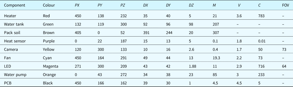
Table 7. Connection points of pipes on components

It is possible to see that most of the sensors are close to their minimum values (see Table 5) in terms of volume, mass, voltage, and current. The only ones that are close to their maximum volume are the pack soil and water tank, which are the ones that we wanted to maximize. The occupied volume is 2,844,316, 28 mm3 which is only 7% of the total volume of the autonomous greenhouse. The weight and energy consumption constraints are also respected since the obtained values are, respectively, 655.8 g and 5.86 W. The presented problem statement of the layout design of a greenhouse is flexible enough to take into consideration physics analysis. For example, gravity can be included in the placement of components to favor the placement of heavy items on the base of the greenhouse, which would make the system more stable. The minimization of the gravitational potential energy could be added as an objective function. Another interesting physical analysis would be a heat analysis, which could help place components and identify missing components in the heat system. For example, the heat analysis based on external and internal parameters could inform the designer if a cooling system is needed. The optimization problem could also include and optimize complexity metrics, which would help define the simplest robust solution.
One of the major issues in the presented algorithm is the parameters of the components are given in terms of the range of values; hence, it is therefore possible to get a solution for which components are not available in the market. Although it remains interesting to keep the parameters of components as a value range, a version of this algorithm could be developed to include a database containing different models of the same component. Furthermore, it would also be possible to change the shape of components from the rectangle approximation that is currently used to a realistic shape of the component based on the dimensions given by the database. It would also give a more precise position of the LOS of components similar to a camera. Another interesting future improvement would be to consider and allow combinations of certain components to minimize the space occupation of components. For example, instead of using a heater and a fan, a compact coaxial fan/heater could be used.
If the simulation parameters presented in Table 4 were to be changed, the output solution is most likely to change. However, the degree of impact on the solution has not been thoroughly studied. Hence, the GA parameters should be optimized to find the ideal simulation parameters using tuning algorithms (Eiben and Smit, Reference Eiben, Smit, Hamadi, Monfroy and Saubion2012; Montero et al., Reference Montero, Riff and Rojas-Morales2018). For example, Ooi et al. (Reference Ooi, Lim and Leong2019) proposed a self-tune linear adaptive GA which modifies the mutation probability rate and the population size based on the diversity of the population. Moreover, the product specifications should undergo a sensitivity analysis to evaluate the robustness of the design.
The optimization problem statement presents many objectives, which can be conflicting. For example, the optimization algorithm needs to minimize the overall volume and to maximize the volume of the pack soil. Currently, these conflicting objectives are implicitly considered by a weighted sum approach in the single-objective optimization. In future work, it is possible to explicitly consider them with a multiobjective optimization without assigning weights to them (Kalyanmoy, Reference Kalyanmoy2001; Simon, Reference Simon2013). By using a multiobjective optimization, a wider range of solutions would be available to the designer to choose from. As mentioned before, the layout design of autonomous greenhouse can also be considered as an MaOP which requires a more sophisticated algorithm to be solved (Hisao et al., Reference Hisao, Noritaka and Yusuke2008; Li et al., Reference Li, Li, Tang and Yao2015; Huang et al., Reference Huang, Zhang and Li2019). However, the selection process of the ideal algorithm to find the best range of solutions needs to be done carefully. Furthermore, the designer would still need to choose one solution among a Pareto-optimal set of solutions given by the multiobjective optimization algorithm using a posteriori approaches (Wang et al., Reference Wang, Olhofer and Jin2017; Yu et al., Reference Yu, Jin and Olhofer2019), which is not a trivial task as reported by Torry-Smith et al. (Reference Torry-Smith, Mortensen and Achiche2011) and Mørkeberg Torry-Smith et al. (Reference Mørkeberg Torry-Smith, Qamar, Achiche, Wikander, Henrik Mortensen and During2012). Also, the presented algorithm rejects automatically a solution that does not respect constraints. Although, it is one way to deal with constraints, other methods based on penalties or the dominating concept could also be used and might yield better results (Kalyanmoy, Reference Kalyanmoy2001).
Finally, the output design of the presented algorithm should be validated by prototyping an autonomous greenhouse. By doing so, new phenomenon or interactions between components could emerge or the importance of one interaction over another could be identified. The algorithm could be then improved, and a new design might be output.
Conclusion
This paper presented how a general problem statement of the layout design of an autonomous greenhouse based on the placement of components is defined and translated into an optimization problem. A GA is then used to solve the optimization problem composed of multiple functional and spatial objective functions and constraints aggregated into a single overall objective using a weighted sum approach. As mentioned before, the problem statement is flexible enough to include physical analysis, such as heat analysis if the designer wants to consider them. Although, the proposed methodology presents weaknesses for the modeling of real components, we deemed that the approximations used in this paper are adequate to give a general idea of the layout design of an autonomous greenhouse and therefore a starting point for a designer. Indeed, we were able to make the design of an autonomous greenhouse for space biology applications where the volume of all the components are 2844, 32 cm3, which is 7% of the total volume. The greenhouse also consumes 5.86 W and weighs 655.8 g, which respect the constraints of the problem statement. Furthermore, the GA is able to output a promising solution by compromising between several spatial guidelines, such as keeping the heat sensor far from the LED and the heater. The GA is also able to find and evaluate an enormous amount of design variations in a reasonable time based on guidelines from the designer. Moreover, the GA can converge toward a near-optimal solution. The validation of the algorithm has yet to be done by prototyping the greenhouse and evaluate its capacity to ensure the plant growth.
Acknowledgments
The authors show their appreciation toward le Fonds de recherche du Québec – Nature et Technologies (FRQNT) and the Canadian Space Agency (CSA) for their financial support.
Yann-Seing Law-Kam Cio is a Ph.D. candidate at Polytechnique de Montréal, Québec, Canada in Mechanical engineering. He received the bachelor and M.Sc. degrees in Biomedical and Mechanical Engineer, respectively, from Polytechnique de Montréal. His research interests are in the field of mechatronics product design, generative design, and evolutionary computation applied to engineering problems.
Yuanchao Ma is a research associate at École Polytechnique de Montréal, Québec, Canada in Mechanical Engineering. He obtained his Master's degree in Mechanical Engineering from INSA Lyon and his M.Sc.A in Aerospace Engineering from Polytechnique de Montréal. His research interests focus on design methodologies, product development, and multi-domain system design.
Aurelian Vadean is Associate Professor at Ecole Polytechnique de Montreal (Canada) in the Mechanical Engineering Department. He teaches Machine design and Mechanical Components Analysis and Optimization course, closely integrated to the capstone project course. He is involved in developing protocols and products for the aeronautic industry and has a valuable experience in design and optimization through his numerous industrial contracts.
Giovanni Beltrame obtained his Ph.D. in Computer Engineering from Politecnico di Milano in 2006. He worked as microelectronics engineer at the European Space Agency on a number of projects, spanning from radiation tolerant systems to computer-aided design. Since 2010, he is a Professor at Polytechnique Montreal with the Computer and Software Engineering Department, where he directs the MIST Lab. His research interests include modeling and design of embedded systems, artificial intelligence, and robotics. He was awarded more than 15 grants by government agencies and industry and has published more than 100 papers in international journals and conferences.
Sofiane Achiche, Ph.D., is a full professor at Polytechnique de Montréal at the Department of Mechanical Engineering. He received the M.Sc.A. and Ph.D. degrees from Polytechnique Montréal, Canada. He is a professor with École Polytechnique de Montréal, Mechanical Engineering Department, Design of Machinery Section. His research interests focus upon evolutionary computational intelligence applied to engineering problems such as condition monitoring. Furthermore, he works in the field of mechatronics design support and mechatronics applied design. He has published over 150 papers in international journals and conferences.


