


1 Introduction
A circular cylinder that undergoes forced in-line cyclic oscillations in steady approaching flow parallel to a stationary plane wall can be found in many practical applications, such as vessel-induced motions of steel catenary risers near touch-down points on the seabed in offshore engineering (Bridge et al. Reference Bridge, Laver, Clukey and Evans2004; Randolph et al. Reference Randolph, Gaudin, Gourvenec, White, Boylan and Cassidy2011). The flow is mainly governed by the free-stream velocity ( $u_{0}$), the cylinder diameter (
 $D$), oscillation amplitude (
 $A$) and oscillating frequency (
 $f_{d}$), the gap distance between the cylinder and the wall (
 $G$) and the boundary-layer thickness
  $(\unicode[STIX]{x1D6FF})$ on the plane wall. These parameters can be normalised based on characteristic length (
 $D$) and velocity (
 $u_{0}$) scales as the Reynolds number (
 $Re=u_{0}D/\unicode[STIX]{x1D708}$), the gap ratio (
 $G/D$) and the boundary-layer thickness ratio (
 $\unicode[STIX]{x1D6FF}/D$). In addition, the cylinder oscillation parameters
  $f_{d}/f_{St}$ and
  $A/D$ are commonly used as characteristic quantities in the literature, where
  $f_{St}$ is the vortex-shedding frequency (or Strouhal frequency) of the otherwise stationary cylinder. The flow characteristics and flow-induced forces on the cylinder are significantly affected by those normalised parameters.
Steady approaching flow around a cylinder near a stationary plane wall has been extensively investigated (e.g. Bearman & Zdravkovich Reference Bearman and Zdravkovich1978; Lei, Cheng & Kavanagh Reference Lei, Cheng and Kavanagh1999; Lei et al. Reference Lei, Cheng, Armfield and Kavanagh2000b). Regular vortex shedding from the cylinder is suppressed when  $G/D$ is smaller than a critical value (Bearman & Zdravkovich Reference Bearman and Zdravkovich1978), which is dependent on
  $\unicode[STIX]{x1D6FF}/D$,
  $G/D$ and
  $Re$. The mechanism for vortex-shedding suppression was ascribed to the interaction of the boundary layer formed on the plane wall and the shear layer developed on the gap-side surface of the cylinder (Lei et al. Reference Lei, Cheng and Kavanagh1999, Reference Lei, Cheng, Armfield and Kavanagh2000b). Wang & Tan (Reference Wang and Tan2008) experimentally investigated the wake flow of a near-wall circular cylinder at
  $Re=12\,000$,
  $\unicode[STIX]{x1D6FF}/D=0.4$ and
  $G/D=0.1{-}1$ by using particle image velocimetry. They observed a distinct asymmetric flow pattern about the cylinder centreline for
  $G/D=0.3{-}0.6$. A critical
  $G/D$ value was reported to be 0.3, beyond which vortex shedding takes place and the normalised vortex-shedding frequency (Strouhal number
  $S_{t}=f_{St}D/u_{0}$) remains roughly constant at 0.19 for
  $G/D$ ranging from 0.3 to 1.
Rao et al. (Reference Rao, Thompson, Leweke and Hourigan2013) numerically investigated the flow past a circular cylinder above a moving wall at the same velocity as the approaching steady flow for  $25\leqslant Re\leqslant 200$ over a wide range of
  $G/D$. The critical
  $Re$ for the onset of three-dimensional (3-D) flow was determined as a function of
  $G/D$. Jiang et al. (Reference Jiang, Cheng, Draper and An2017a) investigated a cylinder near a moving wall in a parameter space of
  $0.1\leqslant G/D\leqslant 19.5$ and
  $Re\leqslant 300$ by using direct numerical simulations (DNS). The flow transition to 3-D occurs at an
  $Re$ value that is smaller than its counterpart for an isolated cylinder (Stewart et al. Reference Stewart, Thompson, Leweke and Hourigan2010; Rao et al. Reference Rao, Stewart, Thompson, Leweke and Hourigan2011). However, flow transition to 3-D for a cylinder near a stationary wall in steady approaching flow has rarely been studied.
Flow around a cylinder undergoing sinusoidal oscillations in the transverse direction of the free stream has been well studied (e.g. Sarpkaya Reference Sarpkaya2004; Williamson & Govardhan Reference Williamson and Govardhan2004). Different flow regimes, such as the 2S regime (two single vortices of opposite signs are formed per oscillation cycle), 2P regime (two pairs of vortices are formed per cycle) and  $\text{P}+\text{S}$ regime (one pair and one single vortex are formed per cycle) are identified in
  $(f_{d}/f_{St},A/D)$ space (Williamson & Roshko Reference Williamson and Roshko1988). Different synchronisation modes, which are referred to as
  $p/q$ modes (
 $p$ and
  $q$ are integers), were discovered. A
  $p/q$ mode flow is characterised by
  $p$ pairs of vortex shedding over
  $q$ periods of cylinder oscillation (Olinger & Sreenivasan Reference Olinger and Sreenivasan1988; Woo Reference Woo1999). The dominant synchronisation mode for a cylinder undergoing sinusoidal oscillations in the transverse direction of the steady approaching flow is
  $1/1$.
Similar to a transverse-oscillating cylinder, synchronisation for a streamwise-oscillating cylinder occurs when the adjusted frequency of vortex shedding ( $f_{s}$) locks onto a rational ratio of
  $f_{d}$, creating a class of flow regimes (e.g. Ongoren & Rockwell Reference Ongoren and Rockwell1988a,Reference Ongoren and Rockwellb; Xu, Zhou & Wang Reference Xu, Zhou and Wang2006; Al-Mdallal, Lawrence & Kocabiyik Reference Al-Mdallal, Lawrence and Kocabiyik2007; Leontini, Lo Jacono & Thompson Reference Leontini, Lo Jacono and Thompson2011, Reference Leontini, Lo Jacono and Thompson2013; Tang et al. Reference Tang, Cheng, Tong, Lu and Zhao2017). Most of the existing studies in the literature have focused on the conditions where the forcing frequency is at or close to
  $2f_{St}$. The forced cylinder oscillation of a frequency in this range leads to the synchronisation of the vortex shedding to the forced oscillation (Griffin & Ramberg Reference Griffin and Ramberg1976). Tang et al. (Reference Tang, Cheng, Tong, Lu and Zhao2017) suggested that the fraction ratios in the Farey sequence in number theory (Farey Reference Farey1816) are all possible
  $p/q$ mode ratios, and that synchronised modes with small values of
  $p$ and
  $q$ are more robust than those with large values of
  $p$ and
  $q$. The primary synchronisation mode for a streamwise-oscillating cylinder is
  $1/2$ (Tang et al. Reference Tang, Cheng, Tong, Lu and Zhao2017). The
  $p/q$ modes with
  $q>2$ are referred to as high-order synchronisation modes, following Pikovsky, Rosenblum & Kurths (Reference Pikovsky, Rosenblum and Kurths2001). For instance, the synchronisation region occupied by mode
  $1/4$ in the
  $(f_{d}/f_{St},A/D)$ parameter space is much wider than that covered by mode
  $3/10$. Interestingly, the synchronised flow also prefers an even-number denominator (
 $q$) to an odd value. For example, the region occupied by mode
  $1/4$ is much wider than that covered by mode
  $1/3$. This phenomenon was ascribed to the spatio-temporal symmetry of the wake of an inline-oscillating cylinder in the free stream. Spatio-temporal symmetry of a flow is defined as
  $\unicode[STIX]{x1D714}_{z}(x,y,\unicode[STIX]{x1D70F})=-\unicode[STIX]{x1D714}_{z}(x,-y,\unicode[STIX]{x1D70F}+T_{M}/2)$, where
  $\unicode[STIX]{x1D714}_{z}$ is the vorticity and
  $T_{M}$ is the period of vortex shedding. Breaking of spatio-temporal symmetry can be induced by either an asymmetric flow geometry about
  $y=0$ or flow instabilities for flows with a symmetric flow geometry about
  $y=0$. Leontini et al. (Reference Leontini, Lo Jacono and Thompson2011, Reference Leontini, Lo Jacono and Thompson2013) and Tang et al. (Reference Tang, Cheng, Tong, Lu and Zhao2017) provided detailed reviews of previous work on this topic and these aspects will not be repeated here. Instead, the flow features in different synchronisation modes are summarised in table 1.
Table 1. Summary of the flow regimes observed around a streamwise-oscillating cylinder.

A streamwise-oscillating cylinder close to a plane wall in steady approaching flow has not been investigated previously. The presence of a plane wall near the cylinder is expected to affect the flow synchronisation modes through the following mechanisms: (i) breaking of spatio-temporal symmetry due to the introduction of the plane wall; and (ii) interaction of wall shear layers with vortices shed from the cylinder. Some works on vortex-induced vibration (VIV) of a near-wall circular cylinder in the transverse direction of the flow exist in the literature (e.g. Tham et al. Reference Tham, Gurugubelli, Li and Jaiman2015; Li et al. Reference Li, Yao, Yang, Jaiman and Khoo2016; Li, Jaiman & Khoo Reference Li, Jaiman and Khoo2017). Although the findings from those studies are relevant, they differ from the present work in two aspects: (1) direction of cylinder oscillation and (2) forced versus induced oscillations.
The primary aim of the present study is to investigate the influence of the wall on the synchronisation modes. A constant  $Re=175$ is chosen in order to make quantitative comparisons with existing results on an isolated cylinder in the literature (Leontini et al. Reference Leontini, Lo Jacono and Thompson2011, Reference Leontini, Lo Jacono and Thompson2013; Tang et al. Reference Tang, Cheng, Tong, Lu and Zhao2017). The numerical model employed in this study is briefly introduced and validated in § 2. The results and discussions are presented in §§ 3 and 4. The 3-D effect on synchronisation modes is investigated in § 5 and conclusions are drawn in § 6.
2 Numerical model
2.1 Numerical method
In this paper, numerical simulations are conducted by discretising the Navier–Stokes equations using the spectral/hp element method embedded in the open-source code Nektar $++$ (Cantwell et al. Reference Cantwell, Moxey, Comerford, Bolis, Rocco, Mengaldo, De Grazia, Yakovlev, Lombard and Ekelschot2015). The dimensionless form of the incompressible Navier–Stokes equations in the Cartesian coordinate system are expressed as follows:
 $$\begin{eqnarray}\displaystyle & \displaystyle \frac{\unicode[STIX]{x2202}\boldsymbol{U}}{\unicode[STIX]{x2202}\unicode[STIX]{x1D70F}}+\boldsymbol{U}\boldsymbol{\cdot }\unicode[STIX]{x1D735}\boldsymbol{U}=-\unicode[STIX]{x1D735}p+\unicode[STIX]{x1D710}\unicode[STIX]{x1D6FB}^{2}\boldsymbol{U}+\boldsymbol{a}, & \displaystyle\end{eqnarray}$$
 $$\begin{eqnarray}\displaystyle & \displaystyle \unicode[STIX]{x1D735}\boldsymbol{\cdot }\boldsymbol{U}=\mathbf{0}, & \displaystyle\end{eqnarray}$$
 where  $\boldsymbol{U}=(u,v,w)$ is the velocity vector,
  $\unicode[STIX]{x1D70F}$ is the time and
  $p$ is the kinematic pressure.
The Nektar $++$ code employs a high-order quadrilateral expansion method within each element through Gauss–Lobatto–Legendre quadrature points (
 $N_{p}$). A second-order implicit–explicit time integration scheme is chosen from the embedded incompressible solver, alongside a velocity-correction splitting scheme and continuous Galerkin projection method. Herein, the harmonic cylinder oscillation is implemented through a moving frame fixed on the cylinder by introducing a forcing term,
  $\boldsymbol{a}$, which is the additional acceleration as the result of the non-inertial translation of the reference frame as detailed by Newman & Karniadakis (Reference Newman and Karniadakis1997). By fixing the coordinate system on the cylinder in the simulation, geometric deformation in the mesh is avoided (Blackburn & Henderson Reference Blackburn and Henderson1999).

Figure 1. The entire domain with a macro mesh for  $G/D=1.0$. The insets are a definition sketch of a cylinder above a plane wall and a close-up view of the element grid near the cylinder.
A definition sketch of the two-dimensional (2-D) problem investigated in the present study is shown in figure 1. The cylinder is forced to oscillate sinusoidally in the  $x$-direction, with its displacement
  $X(\unicode[STIX]{x1D70F})$ and velocity
  ${\dot{X}}(\unicode[STIX]{x1D70F})$ being described as follows:
 $$\begin{eqnarray}\displaystyle X(\unicode[STIX]{x1D70F})=A\sin (2\unicode[STIX]{x03C0}f_{d}\unicode[STIX]{x1D70F}),\quad {\dot{X}}(\unicode[STIX]{x1D70F})=2\unicode[STIX]{x03C0}f_{d}A\cos (2\unicode[STIX]{x03C0}f_{d}\unicode[STIX]{x1D70F})=u_{p}, & & \displaystyle\end{eqnarray}$$
 where  $u_{p}$ represents the velocity of the reference frame.
2.2 Boundary and initial conditions
A rectangular computational domain is employed in the 2-D numerical simulations as shown in figure 1. Along the left boundary, the Dirichlet boundary conditions of  $u=u_{inlet}$ and
  $v=0$ are applied, where
  $u_{inlet}$ is defined as
 $$\begin{eqnarray}u_{inlet}=u_{0}+u_{p}=u_{0}+2\unicode[STIX]{x03C0}f_{d}A\cos (2\unicode[STIX]{x03C0}f_{d}\unicode[STIX]{x1D70F}).\end{eqnarray}$$
 Along the right boundary, the Neumann boundary condition (zero normal gradient) is employed for the velocity (i.e.  $\unicode[STIX]{x2202}u/\unicode[STIX]{x2202}y=0$,
  $\unicode[STIX]{x2202}v/\unicode[STIX]{x2202}x=0$). The cylinder surface is specified as a no-slip boundary with zero velocity (i.e.
  $u=0$,
  $v=0$). A ‘symmetry-wall’ condition (i.e.
  $\unicode[STIX]{x2202}u/\unicode[STIX]{x2202}y=0$,
  $v=0$) is applied at the top boundary.
The presence of a stationary (fixed) plane wall affects the flow around the cylinder through two mechanisms: (i) the boundary layer that is generated above the wall; and (ii) the velocity redistribution due to the wall–cylinder geometry setting, which is referred to as the blockage effect. To differentiate the effects of these two mechanisms, additional simulations are conducted under ‘moving-wall’ and ‘symmetry-wall’ conditions. Apart from  $v=0$, the following boundary conditions are applied on the plane wall:
 $$\begin{eqnarray}\displaystyle & \displaystyle u_{fixed}=u_{p}=2\unicode[STIX]{x03C0}f_{d}A\cos (2\unicode[STIX]{x03C0}f_{d}\unicode[STIX]{x1D70F}), & \displaystyle\end{eqnarray}$$
 $$\begin{eqnarray}\displaystyle & \displaystyle u_{moving}=u_{inlet}=u_{0}+2\unicode[STIX]{x03C0}f_{d}A\cos (2\unicode[STIX]{x03C0}f_{d}\unicode[STIX]{x1D70F}), & \displaystyle\end{eqnarray}$$
 $$\begin{eqnarray}\displaystyle & \displaystyle \frac{\unicode[STIX]{x2202}u_{sym}}{\unicode[STIX]{x2202}y}=0, & \displaystyle\end{eqnarray}$$
 where  $u_{fixed}$,
  $u_{moving}$ and
  $u_{sym}$ are the velocities of the ‘fixed wall’, ‘moving wall’ and ‘symmetry wall’, respectively. A reference value of zero is assigned to the pressure at the outlet (right), and a high-order pressure boundary condition of pressure gradient is imposed on the cylinder surface and the far-field boundaries (Karniadakis, Israeli & Orszag Reference Karniadakis, Israeli and Orszag1991).
Initial conditions of  $u=0$,
  $v=0$ and
  $p=0$ are implemented in all simulations, unless otherwise specified. To eliminate the effect from these initial conditions, more than 600 non-dimensional time units are simulated and the final 400 (approximately 70–300 oscillation cycles) are used to identify synchronisation modes and to estimate the forces on the cylinder. Each 2-D case requires 48 central processing units over 24 h, and over 2000 cases in total are simulated.
2.3 Mesh dependence check and model validation
A dependence check of computational mesh and domain size is conducted at  $G/D=0.5$ and
  $Re=175$ for an oscillating cylinder under both ‘fixed-wall’ and ‘moving-wall’ conditions and the results are detailed in appendix A. A rectangular computational domain of
  $128D\times (28D+G)$ is selected based on the outcomes of the domain size check. A typical mesh with
  $G/D=1.0$ is illustrated in figure 1.
The numerical model is validated by comparing the vortex-shedding frequency and force coefficients from a stationary near-wall cylinder. The vortex-shedding frequency of the near-wall cylinder is defined as  $f_{St^{\ast }}$, to differentiate it from that of an isolated cylinder
  $(f_{St})$. The drag and lift coefficients are defined as follows:
 $$\begin{eqnarray}\displaystyle & \displaystyle C_{D}=F_{x}/(0.5\unicode[STIX]{x1D70C}Du_{0}^{2}), & \displaystyle\end{eqnarray}$$
 $$\begin{eqnarray}\displaystyle & \displaystyle C_{L}=F_{y}/(0.5\unicode[STIX]{x1D70C}Du_{0}^{2}), & \displaystyle\end{eqnarray}$$
 where  $F_{x}$ and
  $F_{y}$ are the total forces on the cylinder in the streamwise and transverse directions, respectively, and
  $\unicode[STIX]{x1D70C}$ is the density of the fluid. The results of
  $f_{St^{\ast }}$ and the mean drag coefficient (
 $C_{D,mean}$) compare favourably with the results reported by Jiang et al. (Reference Jiang, Cheng, Draper and An2017a) under the moving-wall conditions (see table 2). Under the fixed-wall conditions, the results reported by Lei et al. (Reference Lei, Cheng, Armfield and Kavanagh2000b) for
  $Re=200$ and
  $G/D=1.0$ are used to validate the present model (see table 2). The
  $f_{St^{\ast }}$ value from our work is 3 % lower than the value from Lei et al. (Reference Lei, Cheng, Armfield and Kavanagh2000b), possibly because of the different domain widths used in those studies:
  $12D$ in Lei et al. (Reference Lei, Cheng, Armfield and Kavanagh2000b) and
  $28D$ in our work. Generally, our results show good agreements with the available results in the literature.
Table 2. Comparison of the vortex-shedding frequency ( $f_{St^{\ast }}$) and mean drag coefficient (
 $C_{D,mean}$) for a stationary cylinder in steady approaching flow with different
  $Re$ and wall conditions (
 $G/D=1.0$).

3 Stationary near-wall cylinder
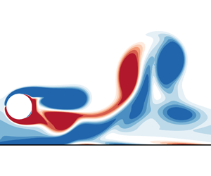
Steady approaching flow around a near-wall stationary cylinder is simulated as a reference for further analysis. Figure 2 shows the flow field at  $Re=175$ over different
  $G/D$ values (0.5, 0.6, 1 and 2) under both fixed-wall and moving-wall conditions. Under fixed-wall conditions (figure 2a–d), the flow field dramatically changes as
  $G/D$ increases, with three different flow regimes identified, as follows.
(i) Regime 1 (
 $G/D\leqslant 0.57$): vortex shedding is completely suppressed. The flow is characterised by stable shear layers that form on the top and bottom sides of the cylinder, as shown in figure 2(a).
(ii) Regime 2 (
$0.57<G/D<2$): vortex shedding from the cylinder is strongly influenced by the plane wall. In this regime, as shown in figures 2(b) and 2(c), the shear layers on both sides of the cylinder roll up to form large-scale vortices and are regularly shed from the cylinder. The vortex street behind the cylinder mostly consists of vortices of negative sense. Vortices of positive sense are primarily cancelled out by the shear layer formed above the plane wall in the gap region.(iii) Regime 3 (
$G/D\geqslant 2$): the flow asymptotes to that around an isolated cylinder with increasing $G/D$. As shown in figure 2(d), the wall shear layer rolls up to interact with the wake of the cylinder at $x/D=5$. Consequently, the wake of the cylinder tilts away from the plane wall. Compared to figure 2(c), vortices of positive sense are less affected by the shear layer on the plane wall.


Correspondingly, the influence of the moving-wall conditions on the flow is quantified in figure 2(e–h). In contrast to figure 2(a–d), the positive shear layer developed on the bottom side of the cylinder surface is hardly affected by the boundary layer on the moving wall and interacts with the negative shear layer to form a well-defined Kármán vortex street at all gap ratios. Thus, the three flow regimes identified under the fixed-wall conditions are not applicable to the moving-wall conditions. Rao et al. (Reference Rao, Thompson, Leweke and Hourigan2013) demonstrated that vortex shedding occurs at  $G/D=0.005$ and
  $Re=200$ under the moving-wall conditions.
The characteristics of the boundary layer at the location of the cylinder are examined by plotting  $u/u_{0}$ against
  $y/D$ (obtained from a separate simulation without the presence of the cylinder) in figure 3. The boundary-layer thickness at the location of the cylinder is calculated based on the vertical distance across the boundary layer from the wall to the point where the flow velocity has essentially reached the maximum. With
  $28D$ from the inlet,
  $\unicode[STIX]{x1D6FF}/D\approx 2$. The
  $f_{St^{\ast }}/f_{St}$ ratios under both fixed-wall and moving-wall conditions for
  $G/D$ up to 10 are also examined in figure 3. Under the fixed-wall conditions,
  $f_{St^{\ast }}/f_{St}$ closely follows the trend of
  $u/u_{0}$, suggesting that the variation in the intrinsic frequency
  $f_{St^{\ast }}$ is mainly due to the difference in the local velocity near the cylinder. Under the moving-wall conditions,
  $f_{St^{\ast }}/f_{St}$ increases with
  $G/D$ much faster than that under the fixed-wall conditions and then decreases asymptotically to the value for an isolated cylinder for
  $G/D>2$. The above results agree with those reported by Jiang et al. (Reference Jiang, Cheng, Draper and An2017a) where a similar variation trend of
  $f_{St^{\ast }}/f_{St}$ was attributed to the changes of local flow rate, induced by the blockage effect of the moving wall.

Figure 2. Wake structure of a circular cylinder in steady approaching flow under fixed-wall (a–d) and moving-wall (e–h) conditions. The vorticity contours are given at levels between  $-1$ (blue colours) and 1 (red colours), with a cutoff level between (
 $-0.2,0.2$). This colour code for vorticity contours is used throughout the paper unless otherwise specified.

Figure 3. Boundary-layer profiles at  $x=0$ (
 $28D$ from the inlet) without a cylinder (solid line) and
  $f_{St^{\ast }}/f_{St}$ of a circular cylinder in steady approaching flow under fixed-wall conditions (circles), alongside that under moving-wall conditions from Jiang et al. (Reference Jiang, Cheng, Draper and An2017a) (dashed line) and the present study (diamonds) over different gap-to-diameter ratios.

Figure 4. Comparison of the average velocity profiles along  $x=0$ with a cylinder placed at
  $(x,y)=(0,0)$ under different conditions.
The velocity profiles with the presence of the cylinder at  $(x,y)=(0,0)$ with different
  $G/D$ and wall conditions are plotted in figure 4, together with that of an isolated cylinder for comparison. Relative to the isolated cylinder, for example at
  $G/D=1.0$, the fixed wall causes a reduction of flow through the gap, whereas the moving wall enhances not only the flow through the gap but also the velocity near the top side of the cylinder. As
  $G/D$ is increased, the flow velocity tends to increase on both sides of the cylinder. The higher local velocities near the cylinder are attributed to the slightly higher
  $f_{St^{\ast }}$ values than those obtained under the fixed-wall conditions at
  $G/D=1.0$, as shown in figure 3.
4 Oscillating near-wall cylinders
Simulations are conducted in the ranges of  $f_{d}/f_{St}\in [1,4]$, with an increment of
  $f_{d}/f_{St}\leqslant 0.02$, and
  $A/D\in [0.01,0.4]$, with an increment of
  $A/D\leqslant 0.1$. We are aware of the possibility that 3-D instabilities may develop at
  $Re=175$ for a near-wall cylinder. It has been demonstrated that 3-D instabilities develop at
  $Re$ of approximately 150–160 for a stationary cylinder next to a moving wall (Rao et al. Reference Rao, Thompson, Leweke and Hourigan2013, Reference Rao, Thompson, Leweke and Hourigan2015; Jiang et al. Reference Jiang, Cheng, Draper and An2017a). To quantify the 3-D effect, additional 3-D simulations are conducted, and the results are reported in § 5.
4.1 Effect of the plane wall
The procedure for classifying synchronisation modes and the naming of the synchronisation modes follow those employed by Tang et al. (Reference Tang, Cheng, Tong, Lu and Zhao2017), where the power spectra of the lift coefficient, a Lissajous phase diagram (cylinder displacement versus lift coefficient) and the flow field were utilised, and the modes were referred to as  $p/q$ modes (such as in figure 5). For clarity, only synchronisation modes with
  $q\leqslant 10$ are differentiated in the present study, and high-order modes (
 $q>10$) are generically defined as other modes (OMs). On the other hand, non-synchronisation modes or quasi-periodic (QP) modes are not discussed extensively, but for completeness are included as
  $\boldsymbol{\cdot }$ in the regime maps (figure 5).
4.1.1 Synchronisation modes
The influence of the plane wall on the synchronisation mode is investigated initially by conducting simulations over two different  $G/D$ (0.5 and 1) and a range of
  $f_{d}/f_{St^{\ast }}$ values at
  $A/D=0.1$ under the fixed-wall conditions. The cylinder is placed
  $28D$ from the inlet, which is identical to the stationary cylinder condition reported earlier. The identified synchronisation modes with
  $A/D=0.1$ are mapped out in figures 5(c) and 5(e). The synchronisation modes at
  $/D=\infty$, reproduced from Tang et al. (Reference Tang, Cheng, Tong, Lu and Zhao2017), are included in figure 5(a) for the purpose of comparison.
To better illustrate the influence of the plane-wall boundary layer on the flow, additional simulations are carried out under the moving-wall conditions, where the plane wall is forced to move at the same velocity as the steady approaching flow. The synchronisation modes are shown in figures 5(b) and 5(d). The corresponding profiles of mean horizontal velocity ( $u_{mean}/u_{0}$), sampled at
  $x=0$ with the cylinder placed at
  $(x,y)=(0,0)$, are shown in figure 4.
The  $f_{St^{\ast }}$ values used for normalisation in figure 5 are the frequencies of vortex shedding around a stationary cylinder at corresponding gap ratios and
  $Re$, which are
  $f_{St^{\ast }}=0.192$ at
  $G/D=\infty$, 0.205 at
  $G/D=1.0$ and 0.198 at
  $G/D=0.5$ under the moving-wall conditions and
  $f_{St^{\ast }}=0.184$ at
  $G/D=1.0$ under the fixed-wall conditions. Since vortex shedding is completely suppressed at
  $G/D=0.5$ under the fixed-wall conditions,
  $f_{St^{\ast }}=0.155$, obtained from
  $G/D=0.6$, is used to normalise
  $f_{d}$ at
  $G/D=0.5$.
Similar to the wake of an isolated oscillating cylinder, a variety of synchronisation modes are revealed as the wall is introduced. There are two major differences in the synchronisation modes. Firstly, the synchronisation modes with an odd number as the denominator ( $q$) of the near-wall cylinder increase significantly, as quantified from the percentage of occurrence, which is determined by the range of synchronisation
  $(f_{d}/f_{St^{\ast }})$ over
  $f_{d}/f_{St^{\ast }}\in [1,4]$. This observation is quite different from that of an isolated cylinder where the modes with even
  $q$ values are the preferred modes. For example, the percentage of occurrence of the
  $1/2$ mode decreases monotonically with the reduction of
  $G/D$ from
  $\infty$ to 1.0 under the fixed-wall conditions, and from 1.0 to 0.5 under the moving-wall conditions, whereas the percentage of occurrence of the
  $1/3$ and
  $2/5$ modes increases noticeably with the reduction of
  $G/D$ from
  $\infty$ to 1 under the fixed-wall conditions. The flow asymmetry around the cylinder, induced by the presence of the walls (stationary and moving), is identified as the physical mechanism for the phenomenon observed above. Consistently, modes with an odd-number denominator (
 $q$) are featured by inclined wakes relative to the flow direction. This reasoning agrees with the interpretation by Tang et al. (Reference Tang, Cheng, Tong, Lu and Zhao2017) that the synchronisation modes for an isolated cylinder prefer an even number to an odd number as the denominator (
 $q$), because modes with an even-number denominator exhibits spatio-temporal symmetry similar to a Kármán vortex street.
Secondly, synchronisation modes with reducible ratios of  $p/q$ (i.e.
  $p$ and
  $q$ have a common factor above 1, such as
  $2/4$ modes) are observed at
  $G/D=1.0$ under the fixed-wall condition. Those modes with reducible ratios of
  $p/q$ have not been reported in the isolated-cylinder case (e.g. Leontini et al. Reference Leontini, Lo Jacono and Thompson2011, Reference Leontini, Lo Jacono and Thompson2013; Tang et al. Reference Tang, Cheng, Tong, Lu and Zhao2017). The
  $2/4$ mode is primarily observed within the parameter space occupied by the primary synchronisation mode of
  $1/2$. Further investigations on the reducible mode ratios are detailed in § 4.1.4.
The synchronisation modes observed with  $G/D=0.5$ under the fixed-wall condition are quite different from other cases, possibly because the suppression of vortex shedding from its stationary cylinder counterpart quenches the occurrence of the modes other than modes
  $0/1$,
  $1/1$ and
  $1/2$.

Figure 5. Locations of the synchronisation modes at  $A/D=0.1$ for: (a)
  $G/D=\infty$ (Tang et al. Reference Tang, Cheng, Tong, Lu and Zhao2017); (b)
  $G/D=1.0$, moving-wall conditions; (c)
  $G/D=1.0$, fixed-wall conditions; (d)
  $G/D=0.5$, moving-wall conditions; and (e)
  $G/D=0.5$, fixed-wall conditions. Here
  $f_{St^{\ast }}$ is the intrinsic vortex-shedding frequency under each condition. The synchronisation modes for
  $q\leqslant 10$ are listed in the legend with increasing value of the mode ratio, while OMs are represented by
  $+$. All cases deemed QP are shown as
  $\boldsymbol{\cdot }$ in the map. The number above modes
  $1/2$,
  $2/5$ and
  $1/3$ is the calculated occurrence percentage from the range of synchronisation
  $(f_{d}/f_{St^{\ast }})$ over
  $f_{d}/f_{St^{\ast }}\in [1,4]$.

Figure 6. Instantaneous vorticity flow field of selected synchronisation modes for an isolated cylinder (a–f) and a near-wall cylinder under moving-wall (g–l) and fixed-wall conditions (m–r) at  $G/D=1.0$. Lissajous phase diagrams of the cylinder displacement versus lift coefficient are shown next to each flow field. From top to bottom: (a,g,m) mode
  $2/3$, (b,h,n) mode
  $1/2$, (c,i,o) mode
  $2/5$, (d, j,p) mode
  $3/8$, (e,k,q) mode
  $1/3$, and (f,l,r) mode
  $1/4$.
4.1.2 Flow characteristics
The instantaneous flow fields of selected synchronised cases are compared in figure 6 through vorticity contours for  $p/q=2/3$,
  $1/2$,
  $2/5$,
  $3/8$ and
  $1/3$ under three different conditions, i.e.
  $G/D=\infty$,
  $G/D=1.0$ under moving-wall conditions, and
  $G/D=1.0$ under fixed-wall conditions.
The wake structures for the near-wall cylinder under the moving-wall conditions are similar to those for an isolated cylinder, especially for modes  $1/2$,
  $2/5$,
  $3/8$ and
  $1/4$. A subtle difference between them is that the wakes for
  $G/D=1.0$ under the moving-wall conditions incline slightly upwards from the wall in the near wake and become approximately parallel to the wall in the far wake, whereas the wakes for the isolated cylinder remain parallel to the free stream and are distributed almost evenly on either side of
  $y=0$. The wake inclinations under the moving-wall conditions are attributable to the positive vertical velocity gradient induced by the strong gap flow, as shown in figure 4. The average velocity directly under the gap is actually larger than the approaching velocity, so that the local flow tends to decelerate (
 $\unicode[STIX]{x2202}u/\unicode[STIX]{x2202}x<0$) as it leaves the gap in the downstream direction, producing an upward velocity component (
 $\unicode[STIX]{x2202}v/\unicode[STIX]{x2202}y>0$) in the near-wall region. The positive vertical velocity gradient will then convect the vortices in the wake upwards.
The widths of the wake for modes with  $p>1$ appear to be larger than for the modes with
  $p=1$ under both isolated and moving-wall conditions. This observation can be explained by considering the interactions of vortices that are generated within
  $p$ pair(s) of vortex shedding in
  $q$ cycles of cylinder oscillation (those within the solid- and dashed-line boxes in figure 6). Only two vortices of opposite signs exist in each box for modes with
  $p=1$, whereas multiple pairs of vortices are present and convected downstream as a group for the cases with
  $p>1$. According to classical vortex dynamics (Saffman Reference Saffman1992), two vortices of opposite signs translate as a unit and two vortices with the same sign rotate around each other. The rotation of vortices with the same sign in the groups of multiple vortex pairs is the direct cause of the wider width of the wake for modes with
  $p>1$.
On the other hand, the most noticeable difference between the wakes obtained under the moving-wall and fixed-wall conditions is that the wakes of the cylinder under the fixed-wall conditions mainly consist of negatively signed vortices that are shed from the top surface of the cylinder, for the same reason as discussed with regard to the results shown in figure 2. In addition, the vortices (with the same sign) in the wakes of modes with  $p>1$ tend to rotate around each other and merge as they are convected downstream, whereas the vortex streets (of opposite signs) in the wakes of modes with
  $p=1$ are almost parallel with the wall without obvious relative rotation or merging of vortices.

Figure 7. Comparison of the instantaneous vorticity flow fields under (a) moving-wall and (b) symmetry-wall conditions at  $(f_{d}/f_{St},A/D,G/D)=(2,0.1,1)$, mode
  $1/2$.
Although the influence of the wall boundary layer on the flow is largely removed by replacing the stationary wall with a moving wall, weak vortices can still be observed on the wall near the cylinder due to the mismatch between the flow velocity in the gap and that of the moving wall. To fully remove the weak vortices on the plane wall, additional simulations are conducted by replacing the moving-wall conditions with symmetry-wall conditions ( $\unicode[STIX]{x2202}u/\unicode[STIX]{x2202}y=0$,
  $v=0$). The instantaneous vorticity flow fields at
  $(f_{d}/f_{St},A/D,G/D)=(2,0.1,1)$ under the moving-wall and symmetry-wall conditions are compared in figure 7. Overall, the wake structures behind the cylinder are very similar under those two boundary conditions, suggesting the negligible effect of the weak vortices on the flow fields behind the cylinder.
4.1.3 Force characteristics
The influence of the plane wall on the drag and lift coefficients ( $C_{D}$ and
  $C_{L}$) is investigated for the cases with
  $A/D=0.1$, as an example. Figure 8 shows the variations of
  $C_{D,mean}$ with
  $f_{d}/f_{St^{\ast }}$ at
  $A/D=0.1$ for the isolated cylinder and near-wall cylinder (
 $G/D=1.0$) under the fixed-wall and moving-wall conditions. Two main features are observed: (i) the
  $C_{D,mean}$ values under the moving-wall conditions and the fixed-wall conditions are consistently larger and smaller, respectively, than those of an isolated cylinder over the range of
  $f_{d}/f_{St^{\ast }}$ investigated here; and (ii) the
  $C_{D,mean}$ values for synchronised flows are generally larger than those of the desynchronised flows in the vicinity of the synchronised flows.
The feature (i) is primarily due to the change of the velocities of the approaching flow local to the cylinder, induced by the presence of two different types of boundary conditions as shown in figure 4. Because  $C_{D,mean}$ is normalised by the free-stream velocity
  $u_{0}$, any change in the velocities of the approaching flow local to the cylinder will be directly reflected by the change in
  $C_{D,mean}$ value. Although only minor differences in the average velocity profiles exist on the top side of the cylinder, a significant increase of flow velocity on the bottom side under the moving-wall conditions leads to an increase of local approaching flow velocity near the cylinder and thus an increase of
  $C_{D,mean}$. Since the gap velocity shows a significant reduction under the fixed-wall conditions, it leads to a reduction of
  $C_{D,mean}$ through the mechanism explained above. If the mean streamwise velocity over
  $y=-1.5D{-}1.5D$ at
  $x=0$ is quantified as a representative value for the approaching flow velocity local to the cylinder,
  $u_{mean}/u_{0}=0.805$, 0.647 and 0.759 are obtained under the moving-wall, fixed-wall and isolated-cylinder conditions, respectively. This result provides a quantitative support to the explanation offered above.
The observed feature (ii) is interpreted by using mode  $1/2$ as an example, where the most pronounced increase in
  $C_{D,mean}$ is observed. This notable increase in
  $C_{D,mean}$ in the region of synchronisation is due to the coalescence of small vortices and, thus, a more organised wake flow, which causes an enhanced shear layer and a stronger entrainment wake (Wu et al. Reference Wu, Lu, Denny, Fan and Wu1998; Tang et al. Reference Tang, Cheng, Tong, Lu and Zhao2017). Slight increases in
  $C_{D,mean}$ can also be observed for other synchronisation modes, but they are not as strong as the increase in
  $C_{D,mean}$ for mode
  $1/2$.

Figure 8. Mean drag coefficient ( $C_{D,mean}$) with respect to
  $f_{d}/f_{St^{\ast }}$ at a fixed
  $A/D=0.1$ for an isolated cylinder (middle line) and near-wall cylinder with
  $G/D=1.0$ under moving-wall conditions (top line) and fixed-wall conditions (bottom line). The same symbols as in figure 5 are also employed here to highlight the influence of synchronisation.

Figure 9. Variations in the mean and r.m.s. of  $C_{L}$ against
  $f_{d}/f_{St^{\ast }}$ at
  $(A/D,G/D)=(0.1,1.0)$ under different wall conditions: (a)
  $C_{L,mean}$, moving-wall conditions; (b)
  $C_{L,rms}$, moving-wall conditions; (c)
  $C_{L,mean}$, fixed-wall conditions; and (d)
  $C_{L,rms}$, fixed-wall conditions. The dashed lines are from the stationary cylinder. The same symbols as in figure 5 are employed.
Figure 9 shows the variations of the mean  $C_{L,mean}$ and the root-mean-square (r.m.s.)
  $C_{L,rms}$ with
  $f_{d}/f_{St^{\ast }}$ under both moving-wall and fixed-wall conditions at
  $(A/D,G/D)=(0.1,1.0)$. The large increase of
  $C_{L,rms}$ in the synchronised modes is induced by the strengthened vortices in the wake at resonance. Each synchronisation mode contains an initial stage (in which
  $C_{L,rms}$ continuously rises), a peak and a desynchronisation stage (where
  $C_{L,rms}$ significantly decreases). The width of the synchronisation range (
 $f_{d}/f_{St^{\ast }}$) is correlated with the magnitude of
  $C_{L,rms}$ under both fixed-wall and moving-wall conditions. The minimum value of
  $|C_{L,mean}|$ in mode
  $1/2$ corresponds to the maximum value of
  $C_{L,rms}$. This behaviour occurs because the strength of vortices that are shed from both sides of the cylinder significantly increases and becomes more uniform at synchronisations. Another interesting phenomenon is the dramatic changes in
  $C_{L,mean}$ and
  $C_{L,rms}$ in figures 9(a) and 9(b) for mode
  $1/3$ under the moving-wall conditions, as detailed in the zoom-in views in figure 10. According to the flow field shown in figure 10, the wakes are tilting away from the plane wall for
  $2.824<f_{d}/f_{St^{\ast }}\leqslant 2.827$ but are more parallel to the plane wall for
  $2.828<f_{d}/f_{St^{\ast }}\leqslant 2.834$. Similar features also exist for an isolated cylinder for mode
  $1/3$ and other modes, with
  $q$ being an odd number (Tang et al. Reference Tang, Cheng, Tong, Lu and Zhao2017).

Figure 10. Instantaneous flow field for an oscillating cylinder near a moving wall at (a)  $(f_{d}/f_{St^{\ast }},A/D,G/D)=(2.827,0.1,1.0)$ and (b)
  $(f_{d}/f_{St^{\ast }},A/D,G/D)=(2.828,0.1,1.0)$, mode
  $1/3$.
4.1.4 Reducible mode ratios
The influence of the plane wall on the synchronisation mode with reducible ratios is investigated by conducting simulations over a range of  $G/D$ and
  $f_{d}/f_{St^{\ast }}$ values at a fixed
  $A/D=0.2$ under the fixed-wall conditions. The identified synchronisation modes with
  $A/D=0.2$ are mapped out in figure 11. The corresponding profiles of mean horizontal velocity (
 $u_{mean}/u_{0}$), sampled at
  $x=0$ with the cylinder placed at
  $(x,y)=(0,0)$, are shown in figure 4. The
  $f_{St^{\ast }}$ values used for normalisation in figure 11 are 0.192, 0.205, 0.197, 0.189, 0.184 and 0.155 at
  $G/D=\infty$, 2.0, 1.5, 1.2, 1.0 and 0.5, respectively, under the fixed-wall conditions.

Figure 11. Locations of the synchronisation modes at  $A/D=0.2$ with varying
  $f_{d}/f_{St^{\ast }}$ and
  $G/D$ under fixed-wall conditions (results at
  $G/D=\infty$ are from Tang et al. (Reference Tang, Cheng, Tong, Lu and Zhao2017) for purpose of comparison). Refer to figure 5 caption for more details.

Figure 12. The spectrum of  $C_{L}$, the transient trace of
  $C_{L}(\unicode[STIX]{x1D70F})$ (red line) with cylinder displacement
  $X(\unicode[STIX]{x1D70F})$ (black line), and the Lissajous phase diagram of
  $X(\unicode[STIX]{x1D70F})$ and
  $C_{L}(\unicode[STIX]{x1D70F})$ for a near-wall cylinder with
  $G/D=1.0$ under the fixed-wall conditions: (a) mode
  $1/2$,
  $(A/D,f_{d}/f_{St^{\ast }})=(0.2,1.292)$; (b) mode
  $2/4$,
  $(A/D,f_{d}/f_{St^{\ast }})=(0.2,1.302)$; (c) QP,
  $(A/D,f_{d}/f_{St^{\ast }})=(0.2,1.323)$; (d) mode
  $3/5$,
  $(A/D,f_{d}/f_{St^{\ast }})=(0.2,1.365)$; (e) QP,
  $(A/D,f_{d}/f_{St^{\ast }})=(0.2,1.386)$; (f) mode
  $4/8$,
  $(A/D,f_{d}/f_{St^{\ast }})=(0.2,1.417)$; (g) mode
  $2/4$,
  $(A/D,f_{d}/f_{St^{\ast }})=(0.2,1.438)$; and (h) mode
  $1/2$,
  $(A/D,f_{d}/f_{St^{\ast }})=(0.2,1.469)$.

Figure 13. Poincaré maps for  $C_{L}$ for a near-wall cylinder with
  $G/D=1.0$ under the fixed-wall conditions (top left to bottom right): mode
  $1/2$,
  $(A/D,f_{d}/f_{St^{\ast }})=(0.2,1.292)$; mode
  $2/4$,
  $(A/D,f_{d}/f_{St^{\ast }})=(0.2,1.302)$; QP,
  $(A/D,f_{d}/f_{St^{\ast }})=(0.2,1.323)$; mode
  $3/5$,
  $(A/D,f_{d}/f_{St^{\ast }})=(0.2,1.365)$; QP,
  $(A/D,f_{d}/f_{St^{\ast }})=(0.2,1.386)$; mode
  $4/8$,
  $(A/D,f_{d}/f_{St^{\ast }})=(0.2,1.417)$; mode
  $2/4$,
  $(A/D,f_{d}/f_{St^{\ast }})=(0.2,1.438)$; and mode
  $1/2$,
  $(A/D,f_{d}/f_{St^{\ast }})=(0.2,1.469)$.
The synchronisation modes found at  $G/D=2.0$ are similar to those found in its isolated-cylinder counterpart, suggesting that the influence of the plane wall is weak at
  $G/D=2.0$. As
  $G/D$ reduces, the synchronisation modes with an odd number as the denominator (
 $q$) increases in the occurrence percentage, which is consistent with the results obtained with
  $A/D=0.1$. Most importantly, synchronisation modes with reducible ratios of
  $p/q$, such as
  $2/4$,
  $4/8$ and
  $4/6$ modes, are observed at
  $0.5<G/D<2$. The modes with reducible ratios of
  $p/q$ have not been reported for an isolated cylinder with similar parameter ranges (e.g. Leontini et al. Reference Leontini, Lo Jacono and Thompson2011, Reference Leontini, Lo Jacono and Thompson2013; Tang et al. Reference Tang, Cheng, Tong, Lu and Zhao2017). Similar to
  $A/D=0.1$, the
  $2/4$ mode is primarily observed within the parameter space occupied by the primary synchronisation mode of
  $1/2$. Interestingly, a transition from the primary synchronisation mode of
  $1/2$ to QP is observed between
  $f_{d}/f_{St^{\ast }}=1.292$ and 1.459 at
  $G/D=1.0$. The transition follows a sequence of 1/2–2/4–QP–3/5–QP–4/8–2/4–1/2 modes. Only synchronisation modes of
  $0/1$,
  $1/1$ and
  $1/2$ are observed with
  $G/D=0.5$ because of the suppression of vortex shedding from its stationary counterpart.
To further investigate the nature of the synchronisation modes with reducible  $p/q$ ratios and the transition from synchronisation modes to QP, the spectrum of
  $C_{L}$, the transient trace of
  $C_{L}(\unicode[STIX]{x1D70F})$ with cylinder displacement
  $X(\unicode[STIX]{x1D70F})$, and the Lissajous phase diagram of
  $X(\unicode[STIX]{x1D70F})$ and
  $C_{L}(\unicode[STIX]{x1D70F})$ for the transition sequence of 1/2–2/4–QP–3/5–QP–4/8–2/4—1/2 modes at
  $G/D=1.0$ are examined in figure 12 with
  $f_{d}/f_{St^{\ast }}$ ranging from 1.292 to 1.469 and
  $A/D=0.2$. The primary synchronisation mode of
  $1/2$ is observed at
  $(A/D,f_{d}/f_{St^{\ast }})=(0.2,1.292)$, as shown in figure 12(a), where the dominant frequency of lift is
  $1/2$ and all other frequencies are integer multiples of frequency
  $1/2$ in the spectrum. The transient trace of
  $C_{L}(\unicode[STIX]{x1D70F})$ completes one cycle of oscillation in exactly two cycles of cylinder oscillation, leading to a closed loop of the Lissajous phase diagram. As
  $f_{d}/f_{St^{\ast }}$ is increased to 1.302, as shown in figure 12(b), the synchronisation mode of
  $2/4$ occurs, where
  $C_{L}(\unicode[STIX]{x1D70F})$ completes two cycles of oscillation in exactly four cycles of cylinder oscillation. Although the dominant frequency of
  $C_{L}(\unicode[STIX]{x1D70F})$ is still
  $1/2$, a lower-frequency component of
  $1/4$ appears, and all other frequencies are integer multiples of frequency
  $1/4$. The Lissajous phase diagram is characterised by two non-overlapping closed loops. The above features of flow response suggest that mode
  $2/4$ is a period doubling of mode
  $1/2$.
As  $f_{d}/f_{St^{\ast }}$ is further increased to 1.323, the flow response (through
  $C_{L}(\unicode[STIX]{x1D70F})$) becomes quasi-periodic (figure 12c), which is characterised by desynchronisation of
  $C_{L}(\unicode[STIX]{x1D70F})$ with
  $X(\unicode[STIX]{x1D70F})$ and non-repeatable loops of the Lissajous phase diagram. Although the dominant frequency in the spectrum of
  $C_{L}(\unicode[STIX]{x1D70F})$ is still
  $1/2$, it is modulated by multiple irregular frequency components. A synchronisation mode of
  $3/5$ occurs surprisingly as
  $f_{d}/f_{St^{\ast }}$ is increased to 1.365, where
  $C_{L}(\unicode[STIX]{x1D70F})$ completes three cycles of oscillation in exactly five cycles of cylinder oscillation (figure 12d). The flow response becomes quasi-periodic again as
  $f_{d}/f_{St^{\ast }}$ is increased to 1.386 (figure 12e). A synchronisation mode of
  $4/8$ appears at
  $(A/D,f_{d}/f_{St^{\ast }})=(0.2,1.417)$, where
  $C_{L}(\unicode[STIX]{x1D70F})$ completes four cycles of oscillation in exactly eight cycles of cylinder oscillation (figure 12f). The mode of
  $4/8$ is judged to be a period doubling of mode
  $2/4$, based on the characteristics of the flow response. The synchronisation mode changes to
  $2/4$ and finally
  $1/2$ again as
  $f_{d}/f_{St^{\ast }}$ is further increased from 1.417 to 1.469 (figures 12g and 12h).
Poincaré maps of  $C_{L}$ are used to show the transition between synchronised and QP states. For a complete cycle of cylinder oscillation, the corresponding value of
  $C_{L}$ was recorded. Thus
  $C_{L}(n)$ is plotted against
  $C_{L}(n-1)$ in figure 13 and
  $C_{L}$ was recorded over 240 cycles of cylinder oscillation. For a synchronised case, the map shows a fixed number (
 $=q$) of points. For example, at
  $(A/D,f_{d}/f_{St^{\ast }})=(0.2,1.292)$ (mode
  $1/2$), two points are shown in the map, while at
  $(A/D,f_{d}/f_{St^{\ast }})=(0.2,1.302)$ (mode
  $2/4$), four points are recorded. On the other hand, in the QP cases, e.g.
  $(A/D,f_{d}/f_{St^{\ast }})=(0.2,1.323)$ and
  $(A/D,f_{d}/f_{St^{\ast }})=(0.2,1.386)$ as shown in figure 13, the points appear randomly distributed over a region and the number of points increases with the recorded time duration, which indicates QP behaviour. Together with the spectrum of
  $C_{L}$ and the Lissajous phase diagram, it is clear that the flow is undergoing a transition from synchronised to QP states.
The response of instantaneous flow fields to the cylinder oscillation is consistent with the response observed through characteristics of  $C_{L}(\unicode[STIX]{x1D70F})$. As an example, figure 14 shows snapshots of vorticity contours of a mode
  $2/4$ case at
  $(A/D,f_{d}/f_{St^{\ast }})=(0.2,1.459)$ over four cycles of cylinder oscillation. The instantaneous flow fields at
  $\unicode[STIX]{x1D70F}=nT$ and
  $\unicode[STIX]{x1D70F}=nT+2T$ would have matched exactly if the synchronisation mode in this case were a
  $1/2$ synchronisation. While the shear layers developed on the surface of the cylinder at
  $\unicode[STIX]{x1D70F}=nT$ and
  $\unicode[STIX]{x1D70F}=nT+2T$ are similar, the interaction patterns
  $(2.5<x/D<7)$ of the vortices shed from the cylinder with the shear layer formed on the wall show an obvious difference at the corresponding instants. It takes two extra cycles of cylinder oscillation for the flow fields to match at
  $\unicode[STIX]{x1D70F}=nT$ and
  $\unicode[STIX]{x1D70F}=nT+4T$. Overall, two pairs of vortices are shed from the cylinder in four cycles of cylinder oscillation, leading to a
  $2/4$ synchronisation in this case. The interaction of the negative shear layer developed on the wall with the positive shear layer developed on the surface of cylinder is evident in figure 14.

Figure 14. Instantaneous flow field of a mode  $2/4$ at
  $(A/D,f_{d}/f_{St^{\ast }})=(0.2,1.459)$ under fixed-wall conditions over four cycles of cylinder oscillation.
The introduction of a wall significantly alters the flow response around the cylinder. Possible influences of the wall on the flow response include (i) the asymmetry of the flow around the top and bottom sides of the cylinder (the mode competition) and (ii) the interaction of the shear layer generated above the surface of the wall with the vortices shed from the cylinder. The blockage effect induced by the presence of the wall leads to the formation of asymmetric shear layers on the cylinder, which subsequently affects the vortex-shedding process from the cylinder. While the interaction of the shear layers formed on the wall with vortices shed from the cylinder is observed in figure 14, the blockage effect of the wall is quantified in figure 15(a) by examining the variation of mean  $u$ velocity component with
  $y$ sampled at
  $x=0$ for the same case as shown in figure 14. The mean
  $u$ velocity component in the gap is noticeably smaller than that on the top side of the cylinder, leading to an asymmetrical approaching flow to the cylinder. We would like to emphasise that the shear layer formed on the wall would also contribute to the flow blockage effect quantified in figure 15(a). The flow asymmetry and the shear layer formed on the wall, nevertheless, are identified as the main causes for the transition to QP through cascade of period doublings.

Figure 15. The  $u$-velocity profiles along the vertical line passing through the cylinder centre
  $(x/D=0)$ at
  $(A/D,f_{d}/f_{St^{\ast }})=(0.2,1.459)$ under (a) fixed-wall condition and (b) symmetry-wall condition.
To separate the influence of the shear layers generated above the surface of the plane wall and the influence of flow blockage effect (to first-order approximation), additional simulations are carried out at  $A/D=0.2$ and 0.3,
  $G/D=1.0$ by imposing a symmetry-wall boundary condition on the plane wall and maintaining other conditions unchanged. The influence of the shear layers generated above the surface of the plane wall can be largely removed with the symmetry-wall condition on the plane wall.
The synchronisation modes mapped out with the symmetry-wall condition at  $A/D=0.2$ and 0.3, shown in figure 16, are clearly different from those obtained under the no-slip boundary condition shown in figure 11. The major differences include: (i) the transition to QP through period doubling of mode
  $1/2$ disappears; (ii) the period doublings of synchronisation modes still exist both inside (mode
  $1/2$) and outside the parameter space otherwise occupied by the primary synchronisation mode of
  $1/2$; (iii) the odds of period doubling of the primary synchronisation mode (
 $1/2$) is increased substantially; (iv) the area covered by the primary synchronisation mode of
  $1/2$ increases substantially and shifts towards to the direction of high
  $f_{d}/f_{St^{\ast }}$; and (v) the synchronisation modes other than
  $1/2$,
  $2/4$,
  $2/3$ and
  $4/6$ largely disappear over the range of
  $f_{d}/f_{St^{\ast }}$ covered in this study. The regime map shown in figure 16 shares certain similarities to that of an isolated cylinder (Tang et al. Reference Tang, Cheng, Tong, Lu and Zhao2017), with a major exception that period doublings of the mode
  $1/2$ were not observed in Tang et al. (Reference Tang, Cheng, Tong, Lu and Zhao2017). The instantaneous flow fields illustrated in figure 17 for the case at
  $(A/D,f_{d}/f_{St^{\ast }})=(0.2,1.459)$ with the symmetry-wall condition on the plane wall show that no shear layers are formed on the plane wall. However, the asymmetry of the shear layers formed on the cylinder still exists, as shown by the variation of mean
  $u$ velocity component with
  $y$ sampled at
  $x=0$ in figure 15(b), albeit the degree of asymmetry is less severe than that observed under the no-slip boundary condition. The average velocity through the gap is slightly larger than that over the top side of the cylinder. The observations suggest that (i) the shear layer formed above the plane wall is responsible for the transition to QP at this
  $A/D$ and (ii) the asymmetry of the mean approaching flow around the cylinder is responsible for the period-doubling behaviours both inside and outside the parameter space otherwise occupied by the primary synchronisation mode of
  $1/2$, based on the comparison of the regime maps with that reported by Tang et al. (Reference Tang, Cheng, Tong, Lu and Zhao2017). To further investigate the influence of the shear layers formed on the wall, simulations are also conducted at
  $A/D=0.2$ and 0.3 under the moving-wall conditions. The flow regime map obtained under the moving-wall conditions (not shown here) is very similar to that shown in figure 16. Although shear layers do form in the vicinity of the cylinder under the moving-wall conditions, the strength and extent of the shear layers are substantially smaller than those observed under the fixed-wall conditions.

Figure 16. The bifurcation diagram plotted with varying normalised excitation amplitude ( $A/D$) and normalised excitation frequency
  $(f_{d}/f_{St^{\ast }})$ at
  $G/D=1.0$ under symmetry-wall conditions.

Figure 17. Instantaneous flow field of a mode  $2/4$ at
  $(A/D,f_{d}/f_{St^{\ast }})=(0.2,1.459)$ under symmetry-wall conditions over four cycles of cylinder oscillation.

Figure 18. The bifurcation diagram plotted with varying shear parameter ( $k$) and normalised excitation frequency (
 $f_{d}/f_{St^{\ast }}$) at
  $A/D=0.2$ for an isolated cylinder in uniform linear shear flow and a near-wall cylinder at different
  $G/D$ under fixed-wall conditions: (a) linear shear flow,
  $k=0.2$; (b)
  $G/D=1.0$, equivalent
  $k=0.13$ (data extracted from figure 11); (c) linear shear flow,
  $k=0.1$; (d) linear shear flow,
  $k=0.05$; and (e)
  $G/D=2.0$, equivalent
  $k=0.02$ (data extracted from figure 11).
The results presented so far (see figures 11 and 16) show that the flow asymmetry and the interaction of the plane-wall boundary layer with vortices shed from the cylinder are two potential culprits for transition to QP through a cascade of period doublings under the fixed-wall conditions. We are, however, still unclear how the level of flow asymmetry affects the flow synchronisation modes. To quantify the influence of the level of flow asymmetry, further simulations are carried out for steady linear shear approaching flow around an isolated cylinder undergoing streamwise oscillations. The shear flow in the simulations is generated by imposing  $u(y)=u_{c}+Ky$,
  $v=0$ on the inlet boundary, where
  $u_{c}$ is the approaching velocity at
  $y=0$ (with
  $x$-axis passing through the centre of the cylinder) and
  $K$ is the transverse velocity gradient. Along the outlet boundary,
  $\unicode[STIX]{x2202}u/\unicode[STIX]{x2202}y=K$ and
  $\unicode[STIX]{x2202}v/\unicode[STIX]{x2202}x=0$ are enforced. A no-slip boundary condition (i.e.
  $u=0,v=0$) is specified on the cylinder surface. Boundary conditions of
  $\unicode[STIX]{x2202}u/\unicode[STIX]{x2202}y=K$ and
  $v=0$ are applied on the top and bottom boundaries, which are located
  $4D$ either side of the centre of the cylinder, following that used by Lei, Cheng & Kavanagh (Reference Lei, Cheng and Kavanagh2000a). The relatively small width of the computational domain is used in order to generate large shear levels in the flow and avoid reverse flow in the computational domain. The shear parameter is defined as
  $k=KD/u_{c}$ and
  $Re$ is defined using
  $u_{c}$. The numerical test is conducted over
  $(f_{d}/f_{st\ast },k)=(1.2{-}2.0,0.05{-}0.2)$ at
  $Re=175$ and
  $A/D=0.2$.
Figure 18 shows the bifurcation diagram plotted with varying  $k$ and
  $f_{d}/f_{St^{\ast }}$ at
  $A/D=0.2$ for an isolated cylinder in a uniform linear shear flow and a near-wall cylinder under the fixed-wall condition. An equivalent
  $k$ value for the near-wall cylinder is determined by
 $$\begin{eqnarray}\displaystyle k=\frac{1}{u_{c}}\int _{G}^{G+D}\frac{\unicode[STIX]{x2202}u}{\unicode[STIX]{x2202}y}\,\text{d}y, & & \displaystyle\end{eqnarray}$$
 with the velocity gradient obtained from the velocity profile given in figure 3, where the cylinder is removed and  $y=0$ is on the plane wall. The equivalent
  $k$ values are 0.13 and 0.02 for
  $G/D=1.0$ and 2.0, respectively. A transition from
  $1/2$ to
  $8/16$ and then to QP is observed for
  $k=0.20$ and
  $f_{d}/f_{st\ast }$ in the range of 1.35–1.37 (as shown in figure 18a). The results shown in figure 18 suggest that the period doubling and transition to QP are indeed
  $k$-dependent. No period doubling occurs in the case with small
  $k=0.05$ in the uniform linear shear flow. The period doubling occurs in both uniform linear shear flow cases with
  $k>0.05$. Although period doubling from
  $1/2$ to
  $2/4$ occurs in reasonably wide bands of
  $f_{d}/f_{st\ast }$ for the cases with
  $k=0.10$ and 0.20, no transition to QP is observed within the Arnold tongue. The above observations appear to support our inference that the interaction of vortex shedding from the cylinder with the plane-wall boundary layer is primarily responsible for the transition to QP through cascade of period doublings inside the Arnold tongue. The transition to QP in the range of
  $1.35<f_{d}/f_{st\ast }<1.37$ mentioned above is outside of the Arnold tongue, which is different from that observed under the fixed-wall conditions. No further attempts are made to increase the
  $k$ value due to the numerical difficulty associated with possible negative velocity near the lower lateral boundary of the computational domain.
The occurrence of flow instabilities inside the otherwise synchronisation region has also been observed previously. For example, Ren et al. (Reference Ren, Cheng, Tong, Xiong and Chen2019) found regime D and F flows (spatio-temporal reflection symmetry breaking) within a region occupied by regime A flow (with spatio-temporal symmetry) at small gap ratios in oscillatory flow around four cylinders in a diamond arrangement. They attribute this strange behaviour to mode competition of the flows through the gaps between the cylinders and around the cylinder cluster. Similar mode completion mechanisms also exist in the cases studied in the present study. This interpretation is somewhat similar to the flow asymmetry discussed in the present study. Li et al. (Reference Li, Yao, Yang, Jaiman and Khoo2016) numerically investigated the VIV of a circular cylinder at  $Re=200$. It was found that the VIV is periodic (
 $1/2$ regime) for an isolated cylinder with reduced velocity of 6.5 and 7, but it becomes quasi-periodic when a plane wall is introduced with
  $G/D=1.0$. It is speculated that the transition to QP of VIV in the case reported by Li et al. (Reference Li, Yao, Yang, Jaiman and Khoo2016) is also strongly related to the shear layer developed on the plane wall. No further investigation is carried out to substantiate this speculation because it is outside the scope of the present study.
4.1.5 Modes with $q>10$ and hysteresis

Tang et al. (Reference Tang, Cheng, Tong, Lu and Zhao2017) demonstrated that more synchronised modes with different  $p/q$ ratios could be identified if the control parameters are further refined. This feature also applies to the near-wall cylinders that are investigated in this study. Table 3 provides a summary of 11 OMs with
  $10<q<20$ at
  $G/D=1.0$ under the moving-wall conditions. For example, a mode of
  $7/18$ is observed at
  $f_{d}/f_{St^{\ast }}=2.497$, which suggests that seven pairs of vortices are shed in
  $18T_{d}$. Figure 19 shows four instantaneous flow structures of mode
  $7/18$ over
  $18T_{d}$. The four inclined dashed lines illustrate a method to separate the groups of vortices. With these inclined dashed lines, we are able to separate the groups of seven pairs of vortices shed in 18 oscillation cycles (mode
  $7/18$). The vortex-shedding process repeats in every 18 cycles of cylinder oscillation. Therefore, by following the four inclined dashed lines, the vortex-shedding process in three successive 18 cylinder oscillation cycles can be observed. This process is essentially the same as the modes with
  $q$ lower than 10.

Figure 19. Instantaneous vorticity contours of mode  $7/18$ for an oscillating cylinder near a moving wall at
  $(f_{d}/f_{St^{\ast }},A/D,G/D)=(2.497,0.1,1)$. Four inclined dashed lines are used to separate the groups of seven pairs of vortices in
  $18T_{d}$.
Table 3. OMs with  $10<q<20$ at
  $G/D=1.0$ under moving-wall conditions.

Hysteresis is checked for three cases near a critical point  $(f_{d}/f_{St^{\ast }},A/D,G/D)=(1.594,0.1,1.0)$ under the fixed-wall conditions, and the results are detailed in table 4. The initial conditions from a fully developed mode
  $1/2$ flow field at
  $(f_{d}/f_{St^{\ast }},A/D,G/D)=(1.594,0.1,1)$ are used to test the hysteresis in these cases. Hysteresis is only found for
  $f_{d}/f_{St^{\ast }}=1.584$, suggesting a very minor hysteresis effect in the wake of the cylinder under forced in-line oscillations based on the limited number of simulations. Further investigations with more simulations are beyond the scope of the present study.

Figure 20. Effect of the oscillation amplitude on the synchronisation modes for a near-wall cylinder at  $G/D=1.0$ under fixed-wall conditions. The shaded areas and dashed lines show the locations of selected modes. Refer to figure 5 caption for more details.
Table 4. Synchronisation mode under different initial conditions.

4.2 Effect of oscillation amplitude
The effect of  $A/D$ on the flow synchronisation mode is illustrated under the fixed-wall conditions with
  $G/D=1.0$, primarily through the map of synchronisation modes in the
  $(f_{d}/f_{St^{\ast }},A/D)$ plane and the frequency content of the lift.
4.2.1 Synchronisation modes
The influence of oscillation amplitude on the synchronisation modes in the  $(f_{d}/f_{St^{\ast }},A/D)$ plane is illustrated in figure 20 for the fixed-wall conditions with
  $G/D=1.0$. A fine increment of 0.01 of
  $f_{d}/f_{St^{\ast }}$ is used for
  $A/D=0.2$ and 0.3 (except for mode
  $0/1$ at
  $A/D=0.3$, where an increment of 0.05 is adopted). Five
  $f_{d}/f_{St^{\ast }}$ ratios are selected (i.e.
  $f_{d}/f_{St^{\ast }}=1.250$, 1.563, 1.876, 2.188 and 2.501), and simulations are conducted with a fine
  $A/D$ increment of 0.01 within
  $A/D\in [0.01,0.4]$. To confirm the boundaries of modes
  $1/3$ and
  $0/1$, the flow with
  $f_{d}/f_{St^{\ast }}=2.897$ is simulated with
  $A/D\in [0.1,0.3]$, and two more cases with
  $f_{d}/f_{St^{\ast }}=3.438$ and 3.959 are simulated with
  $A/D\in [0.2,0.3]$. The shaded areas and dashed lines show the bands of synchronisations, which are referred to Arnold tongues according to Olinger & Sreenivasan (Reference Olinger and Sreenivasan1988).
Generally, three trends are observed on the synchronisation modes as  $A/D$ increases. Firstly, the
  $f_{d}$ value that is required for the occurrence of a certain mode is reduced when
  $A/D$ increases, which is consistent with the results of an isolated cylinder as reported by Tang et al. (Reference Tang, Cheng, Tong, Lu and Zhao2017) and Leontini et al. (Reference Leontini, Lo Jacono and Thompson2013). Secondly, the number of synchronisation cases for certain dominant modes, such as modes
  $2/3$,
  $3/5$,
  $1/2$,
  $3/7$ and
  $1/3$, significantly decreases as
  $A/D$ increases from 0.1 to 0.2. Thirdly, the variety of synchronisation modes decreases with increasing
  $A/D$. For example, modes
  $6/7$,
  $5/6$,
  $4/5$,
  $3/4$ and
  $1/4$ are observed at
  $A/D=0.1$ but not at
  $A/D=0.2$. In addition, modes
  $2/3$,
  $3/5$,
  $3/7$,
  $3/8$ and
  $1/3$ are not found at
  $A/D=0.3$. Tang et al. (Reference Tang, Cheng, Tong, Lu and Zhao2017) pointed out that fine increments are required to systematically capture synchronisation modes composed of relatively large natural numbers of
  $p$ and
  $q$. For relatively small
  $f_{d}/f_{St^{\ast }}$, the reduction of synchronisation modes with increasing
  $A/D$ is again because the modes with very narrow bands of synchronisation require extremely fine increments of
  $f_{d}/f_{St^{\ast }}$. Moreover, at
  $A/D=0.3$ with relatively large
  $f_{d}/f_{St^{\ast }}$, a large area is covered by mode
  $0/1$, which indicates that the flow is dominated by the cylinder oscillation in this regime. The domination of cylinder oscillation is the reason why some of the synchronisation modes, such as modes
  $1/3$ and
  $1/4$, disappeared at this range of
  $A/D$ and
  $f_{d}/f_{St^{\ast }}$.
Two substantial differences are observed by comparing the present regime map with that for an isolated cylinder reported by Tang et al. (Reference Tang, Cheng, Tong, Lu and Zhao2017). Firstly, two large bands of modes  $2/5$ and
  $1/3$ are observed for the near-wall cylinder, while the modes
  $2/5$ and
  $1/3$ bands are extremely narrow for an isolated cylinder. As discussed in the previous section, the flow asymmetry is responsible for the significant increase in synchronisation modes with an odd number as the denominator. Secondly, modes with reducible mode ratios (such as modes
  $2/4$,
  $4/6$ and
  $4/8$) are more pronounced at large
  $A/D$ values. Most of the modes with a reducible ratio (modes
  $2/4$ and
  $4/8$) are found within the range of the primary synchronisation regime, while a few are found outside this range. For example, a couple of mode
  $4/6$ cases are found near mode
  $2/3$. Furthermore, mode
  $2/6$ is found near mode
  $1/3$ at
  $(f_{d}/f_{St^{\ast }},A/D)=(2.501,0.14{-}0.16)$. The period doublings are more pronounced at larger
  $A/D$ values because the vortex shedding due to the cylinder oscillation is enhanced. Another obvious difference is the transition to QP within the boundary of mode
  $1/2$, which was not observed for an isolated cylinder (e.g. Leontini et al. Reference Leontini, Lo Jacono and Thompson2011, Reference Leontini, Lo Jacono and Thompson2013; Tang et al. Reference Tang, Cheng, Tong, Lu and Zhao2017).
4.2.2 Frequency content of the lift
The frequency of lift fluctuations is referred to as the fundamental frequency of vortex shedding in the literature (Williamson Reference Williamson1995). The fundamental frequency of lift is analysed here through fast Fourier transforms. The energy spectra of different frequency components are shown in figure 21 with greyscale contours. The spectra from each value of  $f_{d}/f_{St^{\ast }}$ are stacked next to each other to show the frequency response of the lift for the near-wall cylinder as a function of
  $f_{d}/f_{St^{\ast }}$. The amplitude of each frequency component in the spectrum is normalised by the number of sampling points in each case. The cutoff ranges of the contours are selected to ensure that the frequency components with high energy are shown in the figure. The synchronisation modes are also labelled as a reference. In this work, the change in the vortex-shedding frequency against
  $f_{d}/f_{St^{\ast }}$ is illustrated at
  $G/D=1.0$ and three different
  $A/D$ ratios under the fixed-wall conditions.

Figure 21. Contours of the frequency content of the lift signal as a function of  $f_{d}/f_{St^{\ast }}$ when
  $G/D=1.0$ under fixed-wall conditions with greyscale contours: (a)
  $A/D=0.1$, (b)
  $A/D=0.2$ and (c)
  $A/D=0.3$. The maximum and minimum values of the greyscale shading are 0.2 and 0.002, respectively. Refer to figure 20 for the legend of synchronisation modes.
The strongest frequency component occurs at the fundamental vortex-shedding frequency, which is shown in darker colour in figure 21, accompanied by the sum and difference frequencies of the primary vortex-shedding frequency and driving frequency. A detailed discussion regarding the frequency variation for  $G/D=\infty$ against
  $A/D$ was provided by Leontini et al. (Reference Leontini, Lo Jacono and Thompson2011), and the change in the vortex-shedding frequency as a function of
  $f_{d}$ at
  $A/D=0.1$ was provided by Tang et al. (Reference Tang, Cheng, Tong, Lu and Zhao2017). At
  $A/D=0.1$ (figure 21a), a gradual transition (reduction) process is observed for the dominating frequency (
 $f_{L}/f_{d}$) with increasing
  $f_{d}/f_{St^{\ast }}$. During this gradual transition stage, the flow mode
  $p/q$ changes from
  $1/1$ to
  $1/4$ (reduction). A plateau in the
  $f_{L}/f_{d}$ versus
  $f_{d}/f_{St^{\ast }}$ plot indicates synchronisation to a mode ratio. For example, the flow locks onto mode
  $1/2$ for a large range of
  $f_{d}/f_{St^{\ast }}$ (i.e.
  $f_{d}/f_{St^{\ast }}\in [1.59,2.06]$), onto mode
  $1/3$ for
  $f_{d}/f_{St^{\ast }}\in [2.64,3.01]$, and onto mode
  $1/4$ for
  $f_{d}/f_{St^{\ast }}\in [3.77,3.84]$.
Apart from the primary vortex-shedding frequency ( $f_{s}$), other strong frequencies (light-grey lines) can be observed in figure 21. The first frequency is symmetrical about
  $f_{s}/f_{d}$ with respect to the line
  $f_{L}/f_{d}=0.5$, which is quantified as
  $f_{d}-f_{s}$. The second is
  $f_{d}$, a well-defined line of
  $f_{L}/f_{d}=1$. Similar to an isolated cylinder, all the frequency contents can be expressed as linear combinations of
  $f_{d}$ and
  $f_{s}$ as
  $|\pm \,Mf_{s}\pm Nf_{d}|$. The frequency contents in the range
  $f_{L}/f_{d}\in [1,2],[2,3]$ and so on are the scaled (down) images of
  $f_{L}/f_{d}\in [0,1]$ with weaker energy. The relationships of
  $f_{L}/f_{d}$ versus
  $f_{d}/f_{St^{\ast }}$ are rather similar for
  $A/D=0.1$ and
  $A/D=0.2$, except that the gradual transition occurs earlier for
  $A/D=0.2$. However, the variation in the frequency content of the lift becomes less obvious for
  $A/D=0.3$, and
  $f_{L}/f_{d}$ shows step changes when the regime transitions happen. This phenomenon occurs because the variation in synchronisation modes and the number of QP cases between these regimes significantly decrease due to the high level of disturbances. For mode
  $0/1$,
  $f_{L}/f_{d}\approx 1$ suggests that two pairs of vortices are shed at the same time during one period of cylinder oscillation. Moreover, the lowest frequency content observed at
  $A/D=0.2$ and
  $f_{d}/f_{St^{\ast }}>2.65$ (figure 21b) represents the secondary vortex-shedding frequency (
 $f_{SV}$) of the QP mode. Further analyses for mode
  $0/1$ and the secondary vortex shedding are detailed in § 4.2.3.
4.2.3 Mode $0/1$

For relatively large  $A/D$ and
  $f_{d}/f_{St^{\ast }}$, a large area in the parameter space is covered by mode
  $0/1$. For an isolated cylinder with mode
  $0/1$, a pair of symmetric vortices forms in each cylinder oscillation period (resulting in zero lift), and the vortex shedding from a steady approaching flow is deemed to be fully suppressed (Tang et al. Reference Tang, Cheng, Tong, Lu and Zhao2017). The time sequence for the binary vortex street of an isolated cylinder can be found in figure 2 of Xu et al. (Reference Xu, Zhou and Wang2006). Although the symmetry in the wake is broken when a plane wall is introduced, the
  $0/1$ mode still exists.
A detailed analysis regarding the  $0/1$ mode for
  $G/D=1.0$ is conducted here to understand the wall effect on this particular flow mode under the fixed-wall conditions. Three main features of the
  $0/1$ mode are discussed here:
(i) The boundary line for mode
$0/1$ in figure 20 is plotted in figure 22, together with the data from Tang et al. (Reference Tang, Cheng, Tong, Lu and Zhao2017) and Leontini et al. (Reference Leontini, Lo Jacono and Thompson2013) for an isolated cylinder. The boundary line from Tang et al. (Reference Tang, Cheng, Tong, Lu and Zhao2017) was estimated from the five labelled data points. The comparison in figure 22 indicates that the fixed wall with $G/D=1.0$ does not significantly change the onset condition of mode $0/1$.(ii) The lift is not zero for mode
$0/1$ in the case of a fixed wall at $G/D=1.0$ due to the flow asymmetry with respect to $y=0$. The lift fluctuates periodically with the cylinder oscillations. A typical $0/1$ wake structure for $G/D=1.0$ is shown in figure 23(c), where vortices are shed simultaneously from the bottom and top sides of the cylinder and two nearly parallel shear layers form in the wake, similar to the results reported in Tang et al. (Reference Tang, Cheng, Tong, Lu and Zhao2017). The corresponding temporal variation of lift is shown in figure 24(cii). The Lissajous phase diagram of $X(\unicode[STIX]{x1D70F})$ and $C_{L}(\unicode[STIX]{x1D70F})$ shows a double-lobed structure. The Lissajous phase diagram for mode $0/1$ could also be a single loop, which is similar to that for mode $1/1$. For this reason, the Lissajous phase diagram alone is not sufficient to identify the synchronisation mode of the flow. Both flow patterns and the Lissajous phase diagram are used to identify flow synchronisation modes in this work.(iii) A large area below the
$0/1$ mode region in figure 20 is covered with the QP mode. A secondary wake is observed in the wake for cases with this QP mode. One typical example of the QP mode is shown in figures 23(b) and 24(b), $(f_{d}/f_{St^{\ast }},A/D)=(3.8,0.2)$. In the near wake $(x/D<4)$, the vortices that are shed from the cylinder surface are very similar to those observed in the $0/1$ mode (figure 23c), but further downstream ($x/D>5$), the small vortices that are shed from the cylinder merge into larger vortices and form a new secondary vortex street. The vortex-shedding frequency in the secondary wake is 0.1544, which is 22 % of $f_{d}$. The formation of this secondary vortex street is attributed to the instability of the shear layers in the wake. Similar observations were reported in the wake of a stationary cylinder (Thompson et al. Reference Thompson, Radi, Rao, Sheridan and Hourigan2014). When $A/D$ is further reduced to 0.1, the wake flow regains synchronisation to mode $1/4$, $(f_{d}/f_{St^{\ast }},A/D)=(3.8,0.1)$, as shown in figures 23(a) and 24(a). In the $1/4$ mode, the vortex shedding occurs alternatively in the wake near the cylinder, which is fundamentally different from the other two QP modes.


Figure 22. Boundary line for mode  $0/1$ extracted from figure 20 alongside the boundary line for an isolated cylinder from Tang et al. (Reference Tang, Cheng, Tong, Lu and Zhao2017) and a boundary point from Leontini et al. (Reference Leontini, Lo Jacono and Thompson2013).

Figure 23. Instantaneous vorticity flow fields for a near-wall cylinder under fixed-wall conditions with  $G/D=1.0$: (a) an example case of mode
  $1/4$, with
  $(f_{d}/f_{St^{\ast }},A/D)=(3.8,0.1)$; (b) a QP case with secondary vortex shedding (SVS) after binary vortices (BV), with
  $(f_{d}/f_{St^{\ast }},A/D)=(3.8,0.2)$; and (c) a case of mode
  $0/1$ with BV and parallel shear layers (PLS), with
  $(f_{d}/f_{St^{\ast }},A/D)=(3.8,0.3)$.

Figure 24. The spectrum of  $C_{L}$, the transient trace of
  $C_{L}(\unicode[STIX]{x1D70F})$ (red line) with cylinder displacement
  $X(\unicode[STIX]{x1D70F})$ (black line), and the Lissajous phase diagram of
  $X(\unicode[STIX]{x1D70F})$ and
  $C_{L}(\unicode[STIX]{x1D70F})$ for a near-wall cylinder with
  $G/D=1.0$ under the fixed-wall conditions: (a) mode
  $1/4$,
  $(f_{d}/f_{St^{\ast }},A/D)=(3.8,0.1)$; (b) QP,
  $(f_{d}/f_{St^{\ast }},A/D)=(3.8,0.2)$; and (c) mode
  $0/1$,
  $(f_{d}/f_{St^{\ast }},A/D)=(3.8,0.3)$.
5 Three-dimensional effects
The potential influence of three-dimensionality of the flow on the results obtained in the present study is examined by conducting 3-D simulations with purposely selected parameters. The majority of the 3-D simulations are conducted at  $G/D=0.5$ (the smallest gap investigated in this study), which is chosen because the 3-D effect is likely to peak at a gap ratio near 0.5, based on the findings on a stationary cylinder next to a moving wall (Rao et al. Reference Rao, Thompson, Leweke and Hourigan2013, Reference Rao, Thompson, Leweke and Hourigan2015; Jiang et al. Reference Jiang, Cheng, Draper and An2017a).
To manage the high demands on computing resources, a relatively coarse mesh and short downstream domain length of  $30D$ (
 $1/6$ of the total elements of the 2-D simulations) are used. Firstly, the 2-D mesh is checked at
  $(f_{d}/f_{St},A/D,G/D)=(4,0.1,0.5)$ under fixed-wall conditions. As shown in table 6 of appendix A, good agreement between the results obtained using these two meshes are achieved with identical
  $f_{s}D/u_{0}$ and exactly the same synchronisation mode. The
  $C_{D,mean}$ value varies by less than 1 %, whereas
  $C_{D,std}$ and
  $C_{L,std}$ vary by less than 1.1 % and 2 %, respectively. Therefore, this coarse mesh is selected for the 3-D simulations here. A spanwise length of
  $12D$ with 120 Fourier planes is chosen, based on the finding reported by Jiang et al. (Reference Jiang, Cheng, Draper, An and Tong2016). A random perturbation of amplitude 0.01 is added to both velocity and pressure in the initial conditions. The variation of flow three-dimensionality is further examined with the spanwise kinetic energy
  $E_{z}$, which is defined as
 $$\begin{eqnarray}E_{z}=\frac{1}{2}\int _{V}\left(\frac{w}{u_{0}}\right)^{2}\text{d}V,\end{eqnarray}$$
 where  $V$ is the volume of the entire domain. The
  $Q$ isosurfaces are used to illustrate the 3-D flow structures (Hunt, Wray & Moin Reference Hunt, Wray and Moin1988), where the
  $Q$ function object calculates and stores the second invariant of the velocity gradient tensor, i.e.
 $$\begin{eqnarray}Q={\textstyle \frac{1}{2}}[(\text{tr}(\unicode[STIX]{x1D735}\boldsymbol{u}))^{2}-\text{tr}(\unicode[STIX]{x1D735}\boldsymbol{u}\boldsymbol{\cdot }\unicode[STIX]{x1D735}\boldsymbol{u})].\end{eqnarray}$$
 Flow transition to 3-D for an isolated stationary cylinder in a steady approaching flow occurs at  $Re_{cr}\approx 194$ (Williamson Reference Williamson1996; Jiang et al. Reference Jiang, Cheng, Draper, An and Tong2016). Since the present simulations are conducted at
  $Re=175$, the flow is 2-D without the presence of the plane wall and cylinder oscillations. When the plane wall alone is introduced, the flow is not expected to transit to 3-D because the flow velocity reduction in the boundary layer will lead to a reduction of local flow
  $Re$, especially at
  $G/D=1.0$ where the interesting physical phenomena are observed. To confirm this conjecture, 3-D simulations of a steady approaching flow
  $(f_{d}/f_{St^{\ast }}=0)$ around a near-wall cylinder with
  $G/D=0.5$ and 1.2 are conducted at
  $Re=175$. The results shown in appendix C suggest that the flow remains 2-D in both cases, as evidenced by temporal variations of
  $E_{z}$ that converge to
  $1.13\times 10^{-8}$ and
  $2.32\times 10^{-11}$, respectively.

Figure 25. The Lissajous phase diagram of  $X(\unicode[STIX]{x1D70F})$ and
  $C_{L}(\unicode[STIX]{x1D70F})$ (black for 2-D simulations and red for 3-D simulations), isosurfaces of
  $Q$, spanwise length (
 $L$), synchronisation modes and the time histories of the spanwise kinetic energy
  $E_{z}$ for 3-D simulations at
  $G/D=0.5$ under moving-wall conditions.
To quantify the influence of cylinder oscillations on flow transitions to 3-D, additional simulations over a wide range of  $f_{d}/f_{St^{\ast }}$ are conducted at
  $Re=175$,
  $A/D=0.1$ and
  $G/D=0.5$ under both fixed-wall and moving-wall conditions. The selection of a relatively small
  $A/D=0.1$ for the demonstration here is not expected to alter the conclusion drawn in this section because the major physical phenomena observed at
  $A/D>0.1$ are also observed at
  $A/D=0.1$ (figure 20). The choice of
  $G/D=0.5$ is because transition to 3-D is expected for
  $Re=175$ and
  $G/D=0.5$ in steady approaching flow around a cylinder above a moving wall. The Lissajous phase diagram of
  $X(\unicode[STIX]{x1D70F})$ and
  $C_{L}(\unicode[STIX]{x1D70F})$ (black for 2-D simulations and red for 3-D simulations), isosurfaces of
  $Q$ (
$Q$ ( $Q=\pm 0.8$), the comparison of synchronisation modes and the time histories of
  $E_{z}$ for selected 3-D simulations under moving-wall conditions are shown in figure 25.
The three-dimensionality is first examined at  $G/D=0.5$ under the moving-wall conditions. For a non-oscillating cylinder, as shown in figure 25(a),
  $E_{z}$ increases exponentially with time in the early stage and then stabilises at an equilibrium value. As an example, the time history of
  $w$ at a sampling point of
  $(x/D,y/D,z/D)=(2,1.5,6)$ is plotted together with
  $E_{z}$ in figure 25(a), where the increasing trend of
  $w$ agrees well with that of
  $E_{z}$. The fluctuation of
  $w$ is cancelled when it is integrated to calculate
  $E_{z}$. For the cases that decay to 2-D,
  $w$ decays rapidly to zero, as shown in figure 25(d). The isosurfaces show an ordered mode A structure (spanwise characteristic length
  $L=4D$ of the 3-D flow structure) without dislocations, which is consistent with Jiang et al. (Reference Jiang, Cheng, Draper and An2017b). On the other hand, for oscillating cylinders, although the wake structures do show some 3-D features at relatively low driving frequencies (i.e.
  $f_{d}/f_{St^{\ast }}<1.68$), the synchronised modes identified from 3-D simulations are identical to those observed in 2-D simulations. Interestingly, the 3-D wake structure with
  $L=1.7D$ in mode
  $1/1$ is observed after the wake structure is fully developed, as shown in figures 25(b) and 25(c). The wake structure for QP cases can be relatively regular with
  $L=4D$ at some instants, as shown in figure 25(e), or irregular, as shown in figure 25(f). For relatively large driving frequencies (i.e.
  $f_{d}/f_{St^{\ast }}>1.68$, as shown in appendix C), the wake structure decays to 2-D. The results suggest that cylinder oscillation tends to suppress 3-D instabilities at this particular pair of
  $G/D=0.5$ and
  $A/D=0.1$.
Under the fixed-wall conditions,  $E_{z}$ decays rapidly to zero, following an initial growth stage in some of the cases with
  $f_{d}/f_{St^{\ast }}\neq 0$. The wake structure is exclusively 2-D and the synchronisation modes identified from 2-D and 3-D simulations are identical, including the case with
  $G/D=1.2$ (shown in appendix C). This observation suggests that the influence of the plane wall and cylinder oscillations is not significant enough to cause the flow transition to 3-D over those particular parameter ranges.
A satisfactory agreement between 2-D and 3-D simulation results on the force coefficients is also observed for 2-D and 3-D results on the force coefficients with varying  $f_{d}/f_{St^{\ast }}$ under both moving-wall and fixed-wall conditions (shown in appendix C).
The above results, especially those obtained under the moving-wall conditions, suggest that three-dimensionality of the flow does not significantly affect the identification of flow synchronisation modes for the time period shown here. The conclusions drawn from 2-D simulations are expected to hold for 3-D flows under the parameter ranges of the present study.
6 Conclusions
Two-dimensional numerical simulations are conducted for a near-wall cylinder that undergoes streamwise oscillations with varying oscillation amplitude ( $A/D$) and frequency (
 $f_{d}/f_{St^{\ast }}$) in a steady approaching flow at
  $Re=175$. Different gap-to-diameter ratios (
 $G/D$) are considered to investigate the influence of the wall boundary layer on wake formation around the oscillating cylinder and the hydrodynamic characteristics. The wall effect is also investigated under fixed-wall, moving-wall and symmetry-wall conditions to differentiate the influences of the plane-wall boundary layer and flow asymmetry induced by the geometrical setting. The major conclusions can be summarised as follows.
A variety of synchronisation modes for a wall-bounded cylinder (also referred to as  $p/q$ modes, following Tang et al. (Reference Tang, Cheng, Tong, Lu and Zhao2017)) are identified. The synchronised flow is relatively robust to changes in the controlling parameters for small
  $p$ and
  $q$ values. Although the phenomenon of synchronisation is similar to that of an isolated cylinder, interactions between the cylinder and the boundary layer along the plane wall notably affect the wake formation. As the cylinder is moved closer to the wall, the percentage of occurrence of synchronisation modes with an odd number as the denominator (such as
  $1/3$) significantly increases, in contrast to that of an isolated cylinder, where the synchronised flow prefers an even number as the denominator in the mode ratio (such as
  $1/4$). This behaviour is ascribed to the asymmetric wake formation of the near-wall cylinder. The interaction between vortices shed from the cylinder with the shear layer formed above the plane wall and the flow acceleration through the gap lead to a wake inclined to the free-stream direction and asymmetric vortex shedding from the cylinder.
The period-doubling phenomenon is observed for a near-wall cylinder undergoing streamwise oscillations over certain ranges of parameters investigated in the present study. The breaking of spatio-temporal symmetry, induced by the wall, is identified to be responsible for the phenomenon. Period doubling occurs only when the asymmetry of the flow reaches above a critical level, which can be measured by the velocity gradient in the wall boundary layer.
Transitions to quasi-periodic states through a cascade of period doublings inside the primary synchronisation region are discovered in the present study. Through specifically designed numerical tests (different wall boundary conditions and the linear shear flow), the interaction of asymmetric vortex shedding from the cylinder (due to a geometry asymmetry) and the boundary layer developed on the wall is found to be the primary cause for this phenomenon.
The fixed wall also tends to stabilise the wake formation, as evidenced by the decrease in the variety of synchronisation modes with large  $p$ and
  $q$ values (such as those with
  $q>10$) as the cylinder is moved close to the wall. The flow mechanism associated with this phenomenon is the same as that responsible for the suppression of vortex shedding from a wall-bounded cylinder in steady approaching flow. At small gap ratios, for example in the case of
  $(G/D,A/D)=(0.5,0.1)$, only the three strongest modes (
 $0/1$,
  $1/2$ and
  $1/1$) are present.
The mean values of the drag coefficient and r.m.s. values of the lift coefficient are generally larger in the region of synchronisation than those outside the range of synchronisations. The increases in the force coefficients are more pronounced in relatively wide synchronisation regions with small values of  $q$ than those in narrow synchronisation regions with large
  $q$ values. This behaviour is caused by the enhanced vortices in the wake at resonance and occurs under both moving-wall and fixed-wall conditions. However, the moving wall does appear to increase the drag coefficient compared to a wall-free cylinder, whereas the fixed-wall effectively lowers the drag coefficient, largely due to different ambient flow velocities under different wall conditions.
The frequency contents in the spectrum of lift coefficients are linear combinations of driving and vortex-shedding frequencies in all the synchronised regions. At low forced amplitudes, the transition of the vortex-shedding frequency between modes is a gradual process. The plateaus indicate different synchronised regimes, i.e.  $p/q$ modes, which are interleaved with numbers of quasi-periodic cases. However, large forced amplitudes of cylinder oscillation lead to apparent jumps in the vortex-shedding frequency, corresponding to the jumps in the ratios of
  $p/q$ modes. This is because the variety of synchronisation modes and the number of quasi-periodic modes are significantly reduced when large amplitudes of perturbation (i.e. large forced amplitudes) are introduced.
Although three-dimensionality of the flow develops in some of the cases under the moving-wall conditions, the synchronisation modes identified through 2-D and 3-D simulations remain identical for the cases where 3-D simulations are conducted. This observation suggests that the conclusions drawn from 2-D simulations hold for 3-D flows, at least in the parameter ranges covered in the present study.
Acknowledgements
The authors would like to acknowledge the support from the National Key R&D Program of China (Project ID: 2016YFE0200100). The first author would like to acknowledge the support from the Australian Government and the University of Western Australia, who provided UPA scholarships for a doctoral degree. The second author would like to acknowledge the support from the Australian Research Council through the Discovery Early Career Research Award (DE150100428). The computational resources were provided by the Pawsey Supercomputing Centre with funding from the Australian Government and the Government of Western Australia.
Declaration of interests
The authors report no conflict of interest.
Appendix A
A rectangular computational domain is employed in the 2-D numerical simulations. The domain length in the  $x$-direction is
  $128D$, with
  $28D$ upstream and
  $100D$ downstream of the cylinder. The domain width in the
  $y$-direction is
  $28D$ and
  $G$ on the top and wall sides, respectively. The mesh dependence is checked here under both fixed-wall and moving-wall conditions with a constant
  $Re=175$ and
  $(f_{d}/f_{St},A/D,G/D)=(4,0.1,0.5)$. Four meshes are generated by changing the polynomial order (
 $N_{p}$). As shown in table 5,
  $N_{p}$ varies from 5 to 8, with the total number of cells ranging from 211 232 to 646 898, and the size of the first layer grid next to the cylinder surface varies from
  $0.0060D$ to
  $0.0034D$. The time step was held constant at 0.002 with varying
  $N_{p}$. The Courant–Friedrichs–Lewy (CFL) number is far below 1. Further checks are conducted on mesh 2 by varying the time step (as shown in meshes 2-a and 2-b,
  $\unicode[STIX]{x0394}tu_{0}/D=0.001{-}0.003$), alongside the domain size (as shown in meshes 2-c and 2-d).
Comparisons of the simulation results based on these meshes under fixed-wall and moving-wall conditions are given in tables 5(a) and 5(b), respectively. Excellent agreement between the results from these meshes can be observed. More importantly, an identical flow synchronisation mode is captured by these different meshes. The  $C_{D,std}$ and
  $C_{L,std}$ values vary by less than 0.16 % and 1.27 %, respectively. In table 5(c), mesh 2-d is chosen at mode
  $3/7$, where the flow displays a secondary shedding frequency at
  $1/7$. The values of
  $C_{D,mean}$,
  $C_{D,std}$,
  $C_{L,mean}$ and
  $C_{L,std}$ vary by less than 1 % between the cases of
  $100D$ and
  $200D$. The synchronisation modes and frequency component of the lift are exactly identical. Therefore, the length of the outlet boundary has minimal influence on the results and
  $100D$ is sufficient to visualise the key structures.
These results suggest that a reasonable mesh convergence has been achieved. Mesh 2 is selected conservatively for the rest of the 2-D simulations in this work.
Table 5. Mesh dependence study for three different parameter groups:  $(f_{d}/f_{St^{\ast }},A/D,G/D)=(4,0.1,1)$, fixed-wall conditions (a);
  $(4,0.1,0.5)$, moving-wall conditions (b); and
  $(2.22,0.1,1)$, fixed-wall conditions (c).

Table 6. Comparison of the 2-D and 3-D results for the force coefficient, vortex-shedding frequency and synchronisation mode for  $(f_{d}/f_{St},A/D,G/D)=(4,0.1,0.5)$ under fixed-wall conditions.

A relatively coarse mesh and short downstream length of  $30D$ (one-sixth of the total elements of the 2-D simulations) is used in the 3-D simulations. Firstly, the 2-D coarse mesh is checked at
  $(f_{d}/f_{St},A/D,G/D)=(4,0.1,0.5)$ under fixed-wall conditions. As shown in table 6, good agreement between these two meshes is achieved with identical
  $f_{s}D/u_{0}$ and exactly the same synchronisation mode. The
  $C_{D,mean}$ value varies by less than 1 %, whereas
  $C_{D,std}$ and
  $C_{L,std}$ vary by less than 1.1 % and 2 %, respectively. Therefore, this coarse mesh is selected for the 3-D simulations here. A spanwise length of
  $12D$ with 120 Fourier layers is chosen, based on Jiang et al. (Reference Jiang, Cheng, Draper, An and Tong2016).
Appendix B

Figure 26. Lissajous phase diagrams of  $C_{D}$ versus
  $C_{L}$ for each mode for
  $G/D=1.0$ and
  $A/D=0.1$ under fixed-wall conditions. The value of
  $f_{d}/f_{St^{\ast }}$ is listed in brackets next to each mode.
A range of distinctive modes of flow synchronisations are observed in this work. Following Tang et al. (Reference Tang, Cheng, Tong, Lu and Zhao2017), the flow modes are called  $p/q$ modes. For completeness, Lissajous phase diagrams of
  $C_{D}$ versus
  $C_{L}$ are shown in figure 26 for each mode at
  $G/D=1.0$ and
  $A/D=0.1$ under fixed-wall conditions. The synchronisation modes for
  $q>10$ are also listed, i.e. modes
  $8/11$,
  $8/13$,
  $8/14$ and
  $6/16$. An example of a QP case is also included. As shown in figure 26, the Lissajous phase diagrams are characterised by time-independent enclosed and regular loops for synchronised cases, whereas the loops do not repeat themselves by cycles and may eventually fill the entire phase space for a non-synchronised case.
Appendix C

Figure 27. The time histories of the spanwise kinetic energy  $E_{z}$ for 3-D simulations that decay to 2D: (a)
  $f_{d}/f_{St^{\ast }}=0$, fixed-wall conditions; (b)
  $G/D=0.5$, moving-wall conditions.
Table 7. Comparison of the 2-D and 3-D results on the force coefficients with varying  $f_{d}/f_{St^{\ast }}$ at
  $G/D=0.5$ under (a) moving-wall conditions and (b) fixed-wall conditions.

Three-dimensional simulations of steady approaching flow  $(f_{d}/f_{St^{\ast }}=0)$ around a near-wall cylinder with
  $G/D=0.5$ and 1.2 under fixed-wall conditions are conducted at
  $Re=175$. It is confirmed that the wake structure of both cases decays to 2-D. Moreover, for an oscillating cylinder with relatively large driving frequencies (i.e.
  $f_{d}/f_{St^{\ast }}>1.68$) under moving-wall conditions at
  $Re=175$,
  $A/D=0.1$ and
  $G/D=0.5$, the wake structure also decays to 2-D. The time histories of
  $E_{z}$ for some example cases are shown in figure 27.
As shown in figure 27,  $E_{z}$ decays rapidly to zero for these cases, following an initial growth stage in some of the cases. The wake structure is exclusively 2-D and the synchronisation modes identified from 2-D and 3-D simulations are identical.
Table 7 compares the 2-D and 3-D results on the force coefficients at  $G/D=0.5$ with varying
  $f_{d}/f_{St^{\ast }}$ under both moving-wall and fixed-wall conditions. A satisfactory agreement between 2-D and 3-D simulation results on the force coefficients is observed under both moving-wall and fixed-wall conditions.


