


1. INTRODUCTION
In recent years, single frequency Global Navigation Satellite Systems (GNSS) positioning has become more popular due to the demand from many mass-market applications, such as Unmanned Aircraft Systems (UAS), Location Based Services (LBS) and Connected and Autonomous Vehicles (CAV) (Pinchin et al., Reference Pinchin, Hide, Park and Chen2008). The appeal of single-frequency GNSS positioning is the low cost of hardware and the relatively high performance that can satisfy the requirements of specific applications. For instance, landslide monitoring or structural health monitoring always requires centimetre or better levels of accuracy with a denser monitoring network (Bellone et al., Reference Bellone, Dabove, Manzino. and Taglioretti2016), but expensive geodetic GNSS receivers are unlikely to be used for these purposes. The implementation of intelligent mobility also requires large numbers of low-cost but high-performance tracking devices installed on the moving platforms. These types of applications provide great opportunities but are also significant challenges for GNSS.
Theoretically, if the carrier phase ambiguities are fixed correctly, the baselines could be determined precisely even with single frequency data. One of the most important factors that could affect the performance of GNSS positioning is cycle slip. If all the cycle slips are detected and repaired correctly, better positioning continuity and quality could be achieved. Therefore, a reliable cycle slip detection and repair method plays a crucial role, especially for single frequency GNSS applications.
Currently, different methods for cycle slip detection and repair have been proposed based on the combinations of GNSS raw observations, including the code-phase wide-lane combination (Blewitt, Reference Blewitt1990), phase-phase geometry-free combination (Xu, Reference Xu2007) and Doppler-phase integration (Xiaohong and Xingxing, Reference Xiaohong and Xingxing2012). Also, a series of numerical methods such as wavelets (Collin and Warnant, Reference Collin and Warnant1995), adaptive filtering (Roberts et al., Reference Roberts, Meng and Dodson2002), polynomial regression (De Lacy et al., Reference De Lacy, Reguzzoni, Sansò and Venuti2008), linear functions (Geng et al., Reference Geng, Meng, Dodson, Ge and Teferle2010; Banville and Langley, Reference Banville and Langley2013) and Kalman filtering (Lin and Yu, Reference Lin and Yu2013) have been developed. These methods need dual-frequency or even triple frequency data to mitigate the influence of ionospheric error and eliminate the impact of unknown coordinates that cannot be attained as prior information, especially in kinematic applications.
For cycle slip detection and repair of single frequency data, the coordinates cannot be cancelled through carrier phase geometry-free combination which needs dual-frequency data. Pseudorange observations can be used to build another form of geometry combination, but its observation noise prevents the detection or repair of small cycle slips (Genyou, Reference Genyou2001). Doppler observations can be used to estimate the coordinates. However, this does not perform well when dealing with complex movement of the observation station (Ren et al., Reference Ren, Li, Zhong, Zhao and Shen2011; Carcanague, Reference Carcanague2012). Numerical methods such as wavelet (Dingfa and Jiancheng, Reference Dingfa and Jiancheng1997) and Kalman filter, can be used for coordinate prediction or estimation, but the performance is not perfect if the motion status is complicated.
In this paper, a new cycle slip detection and repair method based on the total differential of ambiguity and Least-Squares Adjustment (LSA) is proposed for single frequency GNSS data. In this method, only L1 carrier-phase observations of two consecutive epochs are processed with LSA to estimate coordinates. Then cycle slip detection is implemented in the positioning domain and the calculated Standard Deviation (STD) is taken as an indicator for detecting cycle slips due to its sensitivity to cycle slips while the estimated coordinates are used for cycle slip repair. The main factors that affect the performance of this method are also analysed using a control variable method.
This paper is organised as follows: the methodology is introduced in Section 2. Section 3 covers the performance assessment of this method applied to process both short and long baselines in the static and kinematic experiments. The conclusions drawn from this work are given in Section 4.
2. METHODOLOGY
The basic equation for the Single Difference (SD) of GNSS carrier phase observations between stations can be expressed as Equation (1):
 $$\lambda \cdot \Phi = R + c \cdot t + T - I - \lambda \cdot N + b + \epsilon$$
where Φ denotes the SD observed carrier phase measurements (cycles); R denotes the SD geometric distance (m); c denotes the speed of light (m/s); t denotes the difference of the clock errors of two receivers (s); T denotes the SD tropospheric delay (m); I denotes the SD ionospheric error (m); λ denotes the carrier phase wavelength (m); N denotes the SD integer carrier-phase ambiguity (cycles); b denotes the SD carrier-phase receiver hardware bias (m) and  $\epsilon$ denotes the SD carrier-phase observation noise (m).
To analyse the characteristic of ambiguity, Equation (1) can be re-arranged as a function of ambiguity after linearisation:
 $$N=(B\cdot X+A-\lambda \cdot \varphi + \epsilon)/\lambda$$
where, B represents the linearisation coefficient matrix; X represents the unknown parameter vector, including the Three-Dimensional (3D) coordinates of the position increments relative to the a priori position for linearization and the clock bias of receivers; A denotes the atmospheric errors including tropospheric delay and ionospheric error; φ denotes the “observed minus computed” carrier phase observable and the other symbols have the same meanings as in Equation (1). For multi-GNSS observations, the satellite-induced phase shift should be taken into consideration if different receivers are used. Although the phase shift bias of the Global Positioning System (GPS) L1 signal that can be estimated or eliminated well is being demonstrated, there are still no unambiguous conclusions about the phase shift of other GNSS systems such as BeiDou (BDS), Globalnaya Navigatsionnaya Sputnikovaya Sistema (GLONASS) or Galileo (Wübbena et al., Reference Wübbena, Schmitz and Bagge2009). The value of phase shift may be variable despite in most cases it being possible to regard it as a constant term. It will be treated as a time-varying variable in this paper. The receiver hardware bias of each GNSS system is different in one multi-GNSS receiver due to the different frequencies and signal structures (Li et al., Reference Li, Ge, Zhang, Nischan and Wickert2013; Reference Li, Zus, Lu, Dick, Ning, Ge, Wickert and Schuh2015a; Reference Li, Ge, Dai, Ren, Fritsche, Wickert and Schuh2015b). In this paper, the influence of phase shift and receiver hardware bias are treated as being absorbed by the clock parameter, so the unknown parameter vector X will contain 3+m parameters if m different GNSS systems are observed.
The cycle slip can be regarded as a total differential of ambiguity, so it can be represented as:
 $$CS=dN=(B\cdot \Delta X+\Delta B\cdot X+\Delta A-\lambda \cdot \Delta \varphi +\Delta \epsilon)/\lambda$$
where CS denotes the cycle slip; dN denotes total differential of ambiguity and Δ denotes the differential values of these variables.
Assume there are two consecutive epochs k and k−1. It is unreasonable to use the same a priori position for linearization in epoch k and k−1 because of the linearization error, particularly in high kinematic situations. Here the linearization coefficient matrix of epoch k−1 can be decomposed into:
 $$B_{k-1} = B_{k} - \Delta B_{k},$$
where ΔB k represents the variation of the coefficient matrix. The cycle slip occurring in epoch k can be expressed as:
 $$\eqalign{CS_{k} &= dN_{k} = (B_{k}\cdot X_{k} - B_{k - 1} \cdot X_{k - 1} + \Delta A_{k} - \lambda \cdot \Delta \varphi_{k} + \Delta \epsilon_{k})/\lambda \cr &= (B_{k}\cdot \Delta X_{k} + \Delta B_{k}\cdot X_{k - 1} + \Delta A_{k} - \lambda \cdot \Delta \varphi_{k} + \Delta \epsilon_{k})/\lambda}$$
where Δ X k can be expressed as:
 $$\Delta X_{k} = X_{k} - X_{k - 1}$$
For applications with a high sampling rate such as a 1 Hz or even higher sampling rate, the influence of the atmospheric error can be neglected even under a very high level of ionospheric activities (Liu, Reference Liu2011; Chen et al., Reference Chen, Ye, Zhou, Liu, Jiang, Tang, Yuan and Zhao2016). However, the atmospheric error cannot be neglected when the sampling interval becomes large. In the discussion below, the applications with a high sampling rate will be preferentially considered in the theoretical derivation, and the influence of atmospheric error will be analysed in the experiment section. Equation (5) can be further simplified as:
 $$\hbox{CS}_{\rm k}=(\hbox{B}_{\rm k}\cdot \Delta \hbox{X}_{\rm k} + \Delta \hbox{B}_{\rm k} \cdot \hbox{X}_{{\rm k} - 1} - \lambda \cdot \Delta \varphi_{\rm k} + \Delta \epsilon_{\rm k})/\lambda.$$
If no cycle slip occurs, Equation (7) can be rewritten as:
 $$B_{k} \cdot \Delta X_{k} + \varepsilon_{k} - \lambda \cdot \Delta \varphi_{k} + \Delta \epsilon_{k} = 0.$$
In Equation (7), εk denotes the term of  $\Delta \hbox{B}_{\rm k}\cdot \hbox{X}_{{\rm k} - 1}$. The value of εk mainly depends on the accuracy of the a priori position of linearization if the sampling interval is constant and the details will be discussed below. To make the illustration and discussion simple, εk is called the linearization error in this paper.
The positioning coefficient matrix B k, for GPS data only, can be expressed as:
 $$B_{k} = \left(\matrix{\matrix{\displaystyle{x_{r}-x^{i} \over \rho_{k}^{i}} &\displaystyle{y_{r}-y^{i} \over \rho_{k}^{i}} &\displaystyle{z_{r}-z^{i} \over \rho_{k}^{i}}\cr \vdots & \vdots & \vdots \cr \displaystyle{x_{r}-x^{m} \over \rho_{k}^{m}} &\displaystyle{y_{r}-y^{m} \over \rho_{k}^{m}} &\displaystyle{z_{r}-z^{m} \over \rho_{k}^{m}}} &\matrix{1\cr \vdots \cr 1}} \right)$$
where x, y, and z denote 3D spatial coordinates of a receiver; subscripts r and k denote the observing station and the serial number of the epoch, respectively; superscripts i and m denote the serial number of observable satellites and ρ is the approximate distance between the a priori position of the station and an objective satellite.
The distance ρ could be changing by about 830 m/s for a static observer and a GPS satellite. However, the rate is quite small. Considering the distance is only used to calculate angles of elevation and azimuths, it can still be regarded as approximately constant at epoch k and k−1 when the sampling interval is not very large, and then:
 $$\Delta B_{k}=\left(\matrix{\matrix{\displaystyle{v_{x}^{i} \over \rho_{k}^{i}} &\displaystyle{v_{y}^{i} \over \rho_{k}^{i}} &\displaystyle{v_{z}^{i} \over \rho_{k}^{i}}\cr \vdots & \vdots & \vdots \cr \displaystyle{v_{x}^{m} \over \rho_{k}^{m}} &\displaystyle{v_{y}^{m} \over \rho_{k}^{m}} &\displaystyle{v_{z}^{m} \over \rho_{k}^{m}}} &\matrix{0\cr \vdots \cr 0}} \right)\cdot dt$$
where v denotes the velocity of the satellite and dt denotes the sampling interval.
To assess the influence of linearization error εk on cycle slip detection, firstly the upper limit of its theoretical magnitude should be evaluated. The a priori position for linearization is always obtained by pseudorange Single Point Positioning (SPP) with metre-level accuracy. Here the externally coincident precision of the a priori position is set to be 10 m. The distance between a station and a satellite could be set to 20,200 km generally for GPS, and the velocity of the satellite can be set to 3·89 km/s. When the sampling interval dt is 1 s we can have:
 $$\varepsilon_{k} = \Delta B_{k} \cdot X_{k-1} \approx {3.89km/s \times 1s \times 10m \over 20200km} \approx 0.0019m \approx 0.01cycle$$
After two differential processing sequences of stations and epochs, the carrier-phase observation noise can be theoretically treated as 0·02 cycles. Hence the influence of εk can be regarded as at the same level of carrier-phase observation noise while the sampling interval is 1 s, but it is obvious that the value of εk will become larger as the sampling interval increases.
It should be mentioned that in kinematic GNSS applications, a sampling rate such as 1 Hz or higher is required, thus the influence of εk can be theoretically neglected, otherwise it needs to be considered while the sampling interval increases to 15 s or even longer. Here, an assumption will be made that the sampling rate is 1 Hz, so the influence of εk can be treated as part of the noise and Equation (8) can be further simplified as:
 $$\lambda \cdot \Delta \varphi_{\rm k} = \hbox{B}_{\rm k} \cdot \Delta \hbox{X}_{\rm k}+\Delta \epsilon_{\rm k}$$
Equation (12) can be treated as a classical LSA model that is similar to the GNSS positioning model by using carrier-phase observations.
The variance-covariance matrix D of X in Equation (12) can be expressed as:
 $$D = \left[\matrix{\matrix{\sigma_{x}^{2} &\sigma_{xy} &\sigma_{xz}\cr \sigma_{yx} &\sigma_{y}^{2} &\sigma_{yz}\cr \sigma_{zx} &\sigma_{zy} &\sigma_{z}^{2}} &\matrix{\sigma_{xT}\cr \sigma_{yT}\cr \sigma_{zT}}\cr \matrix{\sigma_{Tx} & \sigma_{Ty} & \sigma_{Tz}} &\sigma_{T}^{2}} \right]$$
where σxσyσzσT denote the STD of x, y, z coordinates and single difference clock error of receivers, respectively. The STD of position σP can be denoted as  $\sigma_{P}=\sqrt{\sigma_{x}^{2}+\sigma_{y}^{2}+\sigma_{z}^{2}}$. If no cycle slip occurs its value should be several centimetres, otherwise it could lead to a large jump of σP. Therefore, a threshold should be set up so that once σP becomes larger than this threshold, the current epoch can be treated as having a cycle slip.
If n satellites of m GNSS systems are observed, the unknown vector X in Equation (12) contains 3+m terms include x, y, z coordinates and m clock parameters, so the degree of freedom of Equation (12) is n-m-3. To calculate the unknown parameter X, it needs at least m+4 equations with no cycle slips to build a Least Squares Adjustment (LSA) equation. The purpose of cycle slip detection and repair is to attain the final precise positioning solution which also needs at least m+4 satellites to build a LSA system, so the condition for cycle slip repair just meets the same requirement with final positioning. Furthermore, since multi-constellation GNSS data is now widely used, this condition would not be too difficult to meet since more and more satellites can be observed (Li et al., Reference Li, Ge, Dai, Ren, Fritsche, Wickert and Schuh2015b). Assuming that the number of satellites in common view with no cycle slip occurring is l (l ≥ m+4) the equation below can be built by using the observations of these l satellites:
 $$\lambda \cdot \Delta \varphi_{k}^{\prime}=B_{k}^{\prime}\cdot {\Delta X}_{k}^{\prime}+\Delta \epsilon_{k}^{\prime}$$
where the superscript “′” denotes the satellites with no cycle slip. To distinguish different STD obtained by Equations (12) and (14), two definitions are given:
Type 1 STD: the STD calculated through Equation (12), which uses the observations of all the satellites.
Type 2 STD: the STD calculated through Equation (14), which uses the observation of the satellites without cycle slips.
The number of all common-viewed satellites is n (n ≥ l), thus the theoretical value of carrier phase observations of these m satellites  $\Delta \varphi_{\rm k}^{\prime\prime}$ can be represented as:
 $$\Delta \varphi_{k}^{\prime\prime}=B_{k}\cdot \Delta X_{k}^{\prime}/\lambda$$
Thus, the cycle slip can be represented as:
 $${CS}_{k} = Int(\Delta \varphi_{k}^{\prime\prime} - \Delta \varphi_{k})$$
where  $\Delta \varphi_{k}^{\prime\prime} - \Delta \varphi_{k}$ represents the float residual obtained by this method. Int denotes the rounded processing. Here, we assume the observation of each satellite is independent and no cycle slip or multipath error affects the observation.
  $\Delta \varphi_{k}^{\prime\prime} - \Delta \varphi_{k}$ represents the least square residuals V and the posterior standard error of unit weight
  $\widehat{\sigma_{0}}$ can be calclulated:
 $$\widehat{\sigma_{0}} = \sqrt{{V^{T}\cdot P\cdot V \over n-m-3}}, \quad V=\Delta \varphi_{k}^{\prime\prime} - \Delta \varphi_{k},$$
where P denotes the weight matrix. The standard error of unit weight can reflect the observation accuracy of carrier phase observations with the value of several millimetres (Liu, Reference Liu2011; Chen et al., Reference Chen, Ye, Zhou, Liu, Jiang, Tang, Yuan and Zhao2016). The value of V should fit a Standard Normal Distribution (SND) with μ=0,  $\sigma _{V}=\widehat{\sigma_{0}}$, where μ and σV denote the expectation and standard deviation of the SND (Kirkko-Jaakkola et al., Reference Kirkko-Jaakkola, Traugott, Odijk, Collin, Sacs and Holzapfel2009). Once an integer cycle slip occurs, the change of system redundancy n−m−3 is neglected, the value of V of the satellite with a cycle slip that is calculated by Equation (16) should fit a SND with μ=Y,
  $\sigma_{V} = \widehat{\sigma_{0}}$, where Y denotes the integer value of the cycle slip. For cycle slip detection, once the cycle slip occurs, it will lead to a change in order of magnitude of the corresponding residual V from several millimetres to 19 cm or even larger with one-cycle slip, and finally cause a large jump in the STD
  $\widehat{\sigma_{0}}$. Normally the magnitude of
  $\widehat{\sigma_{0}}$ is several millimetres and it will become larger if the multipath and atmospheric error is considered (Liu, Reference Liu2011; Chen et al., Reference Chen, Ye, Zhou, Liu, Jiang, Tang, Yuan and Zhao2016) and
  $3\widehat{\sigma_{0}}$ is always used as a threshold to judge the abnormal values with a 99·73% confidence level. In this paper, the empirical threshold of STD is set to 0·05 m after a large amount of data processing and a review of relevant literature (Blewitt, Reference Blewitt1989). It is slightly larger than
  $3\widehat{\sigma_{0}}$, but performs better and can avoid the epochs with no cycle slip being wrongly judged as with cycle slips when the observation environment is not perfect. For cycle slip repair, theoretically the absolute value of the fractional part of V should be in the range of
  $[-3\widehat{\sigma_{0}}, 3\widehat{\sigma_{0}}]$. Assuming the float value of the residual is βf and it can be rounded to an integer βInt, if the absolute value of
  $\vert \beta_{f}-\beta_{Int} \vert $ is smaller than 0·2, it will be regarded as a cycle slip. It should be mentioned that in order to identify the half-cycle slips, an empirical value of 0·05 cycles is selected as the threshold in this paper, which means if the fractional part of CS k is in a range of 0·45 to 0·55 cycles, thus CS k can be regarded as a half-cycle slip.
3. EXPERIMENT AND VALIDATION
As mentioned, linearization error ε and atmospheric errors Δ A play the main roles in this method. In this paper only GPS data is used to assess their effects. Firstly, the performance was assessed under different conditions based on a control variable method of which the impact of linearization error ε and atmospheric errors Δ A will be assessed step by step and two sets of experiments using static short and long baselines were carried out.
Table 1 shows the detailed arrangements that were covered in the following cases for the assessments, where × denotes that a particular factor (ε, Δ A) can be neglected in a discussion of this section, ✓ represents this factor should be considered in this case, and the column of comments indicates whether the data is static or kinematic.
Table 1. Experiment Arrangement.

A short baseline of approximately 2 m was used to investigate the impacts of linearization error ε. Using the experimental data of different sampling intervals (1 s, 15 s, 30 s and 60 s) and high- (of a few mm obtained by post-processing) and low-accuracy (of about 10 m obtained by SPP) initial coordinates assessments are carried out in Case 1 and 2, respectively. The data was collected on 20 February 2013 from 04:00 for about 2 hours and cut-off angle was set to 10°. The accurate baseline was calculated by post-processing and the integer ambiguity of each satellite at each epoch was also fixed, when no cycle slips are found. All these results can be taken as the ground-truth reference.
In the long baseline experiments, a baseline of approximately 289 km was selected, where the atmospheric errors must be considered. The data on 9 March 2013 from 0:00 to 2:00 was collected at 1Hz. The coordinates are estimated with GPS Analysis at Massachusetts Institute of Technology (GAMIT) software (http://www-gpsg.mit.edu/~simon/gtgk/) and the International GNSS Service (IGS) precise orbit and clock products were utilised in data processing. The same sampling intervals and initial coordinates of similar levels of accuracy were used in the assessments. The atmospheric errors play a major role while the initial coordinates of centimetre accuracy were used in Case 3. Since the tropospheric delays are relatively stable over a short period, the impact of the ionospheric error on the performance of this method was assessed. Δ A and ε affect the performance of this method when the initial coordinates of metre-level accuracy were used in Case 4.
To further assess the performance of the proposed method, kinematic data sets collected from short- (0–20 km), medium- (20–50 km) and long-baselines (>50 km) were also processed in Case 5. Since high-rate GNSS data are required for kinematic applications (Cramer et al., Reference Cramer, Stallmann and Haala2000; Meng et al., Reference Meng, Roberts, Dodson, Ince and Waugh2006), only 1 Hz kinematic data was used in this experiment, and theoretically, the effect of linearization modelling error and atmospheric error are insignificant according to the earlier discussion.
It should be mentioned that in practical applications, the atmospheric error impact or other effects such as multipath or satellite orbit errors cannot be weakened or eliminated by the single-difference between stations with the increasing length of baseline, so the positioning accuracy by using single-frequency carrier phase observations will be decreased or become even unavailable since the fixed integer carrier phase ambiguities cannot be obtained with large SD residuals of atmospheric errors. This paper only aims at the illustration of cycle slip detection and repair performance of the proposed method, and the positioning performance is not discussed.
For the Case 1 to Case 4 experiments, cycle slips are artificially added to make a good reference for further analysis. These cycle slips are added epoch by epoch. For each epoch, the basic rule is: a full cycle slip is added while the number of common-viewed satellites between two consecutive epochs is larger than five and a half-cycle slip is added when the number of common-viewed satellites is larger than six. This means that for each epoch there are two satellites containing cycle slips if the number of common-viewed satellites is equal or greater than seven. It should be noted that the bit change of the navigation message modulated on the signal may also cause a half-cycle slip if the receiver does not or fails to decode navigation data properly, so the half-cycle slip needs to be considered (Kirkko-Jaakkola et al., Reference Kirkko-Jaakkola, Traugott, Odijk, Collin, Sacs and Holzapfel2009). After the cycle slip detection and repair at the current epoch, the carrier phase observables will be recovered to their original values, and then the experiment of the current epoch will have no influence to the experiments of subsequent epochs.
In the relevant figures below (Figures 4, 7 and 9), different colours are used to mark the artificially added cycle slips of the epochs to clearly display the cycle slip repair performance. Finally, the success rate of the repair will be statistically summarised. If a total of n half- or full-cycle slips are added, and m of them are repaired successfully based on the threshold we set, so the success rate is calculated as m/n, and the number of success rate, m and n are listed in Table 3 and other related discussion parts.
3.1. The analysis of STD with no cycle slips
As discussed above, the STD of Equation (12) is taken as an indicator to judge whether a cycle slip occurs. Theoretically, the abnormally large STD would appear at the epochs that contain cycle slips. First of all, the STD with no cycle slips was estimated and statistically analysed from Case 1 to Case 4.
As shown in Figure 1, all the STD values with 1 s and 15 s sampling interval are smaller than 0·05 m. Normally the threshold for cycle slip detection can be set as Max(σP) below with 99·73% confidential level:
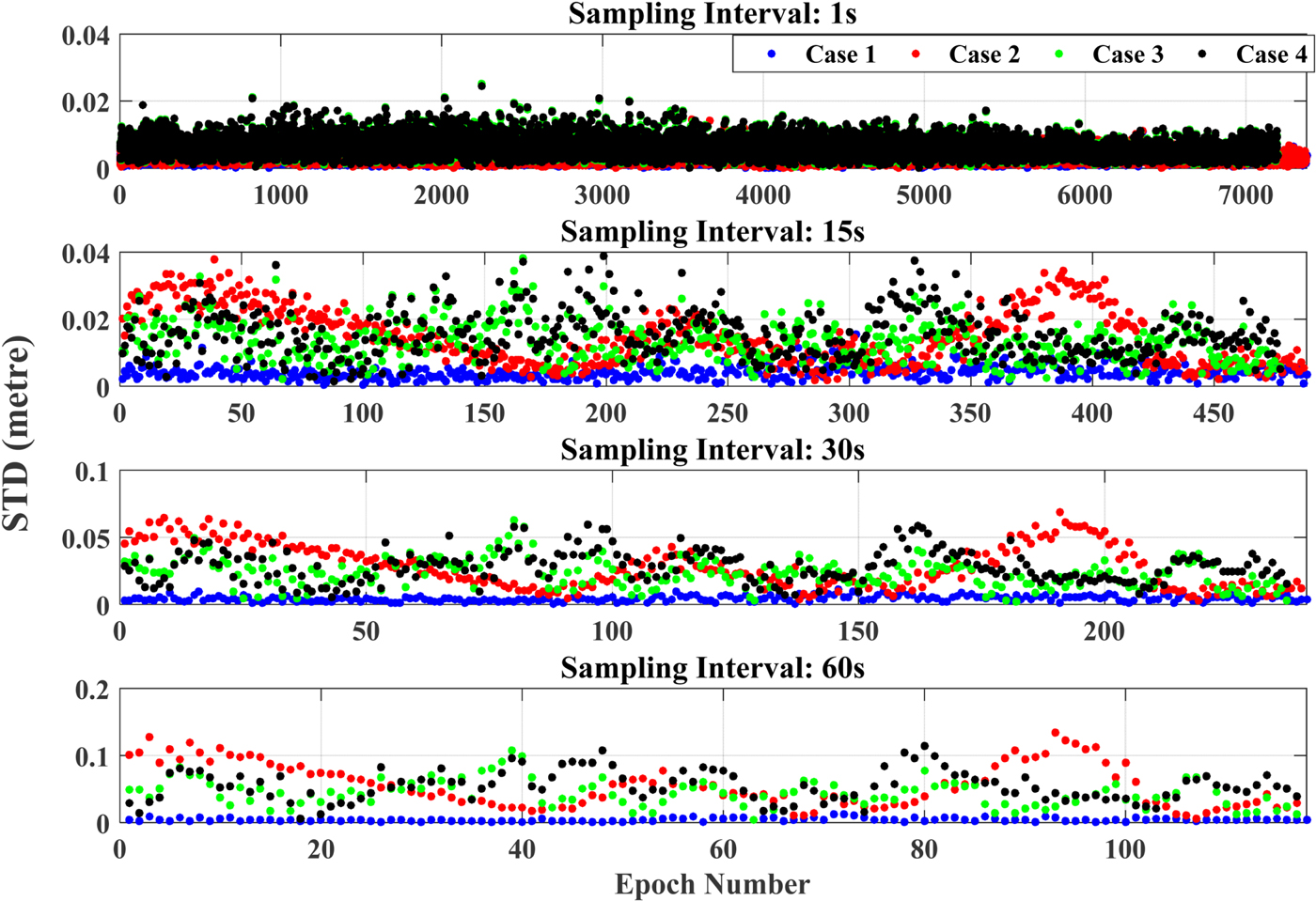
Figure 1. STD values of Case1 to Case 4 with different sampling intervals (no cycle slips).
 $$Max(\sigma_{P}) = Mean(\sigma_{P}) + 3 \times STD(\sigma_{P})$$
The statistical values of σP are included in Table 2. This also demonstrates that while the sampling interval is 1 s or 15 s, 0·05 can be a proper threshold for cycle slip detection in this paper. However, the influence of the linearization error ε and atmospheric error Δ A will increase with a larger sampling interval, which will lead to the failure of cycle slip detection. Therefore, the experiments with only 1 s and 15 s sampling intervals are considered in this paper for Cases 2, 3 and 4, otherwise the epochs with no cycle slip may be incorrectly classified as with cycle slips if the sampling intervals are 30 s or even longer. For Case 1, all the sampling intervals should be discussed since theoretically the linearization and atmospheric error has nearly no effect and the statistical information in Table 1 also verifies this. It is also interesting that with a 15 s sampling interval, the Max(σP) values of a Case 4 sampling interval are slightly larger than that of Case 3, but the Max(σP) value of Case 2 is significantly larger than that of Case 1. The major reason is the accuracy of the initial coordinates obtained by SPP has been improved by using the precise products of IGS which weaken the impact of linearization error.
Table 2. Statistical information of STD with no cycle slip (unit: metre).

3.2. Short baseline experiments
To assess the performance of this method, one-cycle slip and a half-cycle slip are added to the PRN24 and PRN9 satellites based on the principle above since these two satellites were observed in the whole observation session and experienced a large variation of elevation angles.
3.2.1. Case 1 experiment (high-accuracy initial coordinates)
Once the cycle slips are artificially added, the STD values significantly increase as shown in Figure 2. It is apparent that the cycle slips will be detected 100% successfully by using the threshold of 0·05 m. Figure 3 shows the detailed information of common-viewed satellites between two consecutive epochs, and it can be seen that the STD values have a strong positive correlation with the values of Position Dilution Of Precision (PDOP). The discontinuity of the STD values in Figure 2 is caused by the change of satellites.
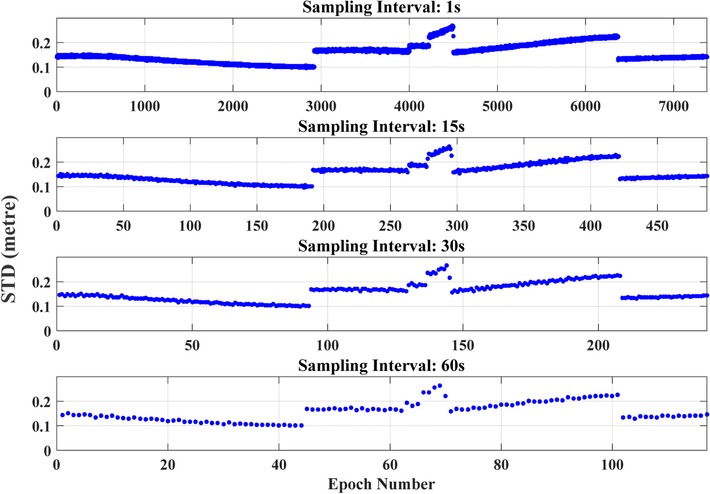
Figure 2. STD values with artificially added cycle slips.

Figure 3. Detail information of satellites in common-view.
As described by Equations (14) to (16), the repair work needs at least five satellites without cycle slips to calculate the unknown parameters ΔX k′. Then the float residual of each satellite in common-view will be obtained based on Equation (15). Figure 4 exhibits the float residuals of all the satellites.

Figure 4. Float residuals of the satellites (PRN24 and PRN9) with and without cycle slips. The red and green points represent the float residual of PRN24 (one-cycle slip) and PRN9 satellite (half-cycle slip), respectively. The blue points represent the float residuals of other satellites.
The cycle slip repair is done with the rule discussed at the end of Section 2, and the repair success rates of one-cycle and a half-cycle slips in terms of 1 s and 15 s sampling intervals of Case 1 are summarised and listed in Table 3 with Cases 2, 3 and 4. When the sampling intervals are 30 s and 60 s, the repair success rates of one-cycle slip/half-cycle slip can reach 100% (239/239)/100% (224/224) and 100% (116/116)/100% (109/109), respectively. All these results show the performance of this new method while the effect of linearization error ε and atmospheric errors Δ A can be neglected.
Table 3. Cycle slip repair success rate of one-cycle slip and a half-cycle slip of Case 1 to Case 4.

3.2.2. Case 2 experiment (low-accuracy initial coordinates)
For Case 2, the linearization error should be taken into consideration. Firstly, the PRN24 satellite is employed to estimate the magnitude of ε, which is shown in Figure 5.

Figure 5. Magnitude of ε of PRN24 satellite.
It is quite clear that the magnitude of ε has a linear relationship with the sampling intervals. When the sampling interval is 1 s, the magnitude of ε is at the level of the measurement noise. However, the value of ε will reach 0·2 cycles with a 30 s sampling interval, and it will be large enough to prevent successful cycle slip detection or even repair. Thus, only 1 s and 15 s sampling intervals will be discussed in this section, which have also been demonstrated in Section 3.1.
As shown in Figure 6, while the sampling interval was 1 s or 15 s, even a half-cycle slip can be detected with the threshold 0·05 m. The process of cycle slip repair is the same as the procedure introduced in Section 3.2.1. The detailed distribution of the float residuals of all the satellites is displayed in Figure 7.
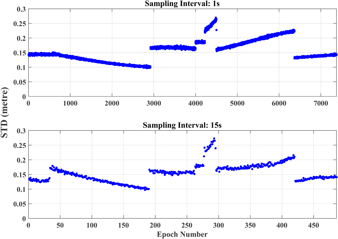
Figure 6. STD values with artificially added cycle slips.

Figure 7. Float residuals of all the satellites in common-view. The red and green points represent the float residual of PRN24 (one-cycle-slip) and PRN9 satellite (half-cycle slip), respectively. The blue points represent the float residuals of other satellites.
According to the repair success rate in Table 3, it is quite obvious that the 15 s would be the maximum value of the sampling interval for the one-cycle slip repair with a 99·2% success rate because of the influence of the linearisation error ε. Meanwhile, the success rate of half-cycle slip repair is just 63·6% with a 15 s sampling interval. Therefore, it is better to detect and mark the half-cycle slips rather than repair them since it would appear to be impossible to judge whether they are half-cycle slips.
3.3. Long baseline experiments (Case 3 and Case 4)
In this section, the performance of this new method is investigated for long baseline applications. Since it is difficult to 100% confirm whether this data is clean without cycle slips, one-cycle slip and a half-cycle slip are added artificially into the raw observations of PRN26 and PRN10 satellites since these two satellites are visible over the whole observation session. The experiments will focus on the changes of STD values caused by the artificially added cycle slips, and according to the discussion in Section 3.1, only 1 s and 15 s sampling intervals will be discussed. Following the experimental procedure of Section 3.2, the STD values with cycle slips of both Case 3 and Case 4 are calculated and displayed in Figure 8.
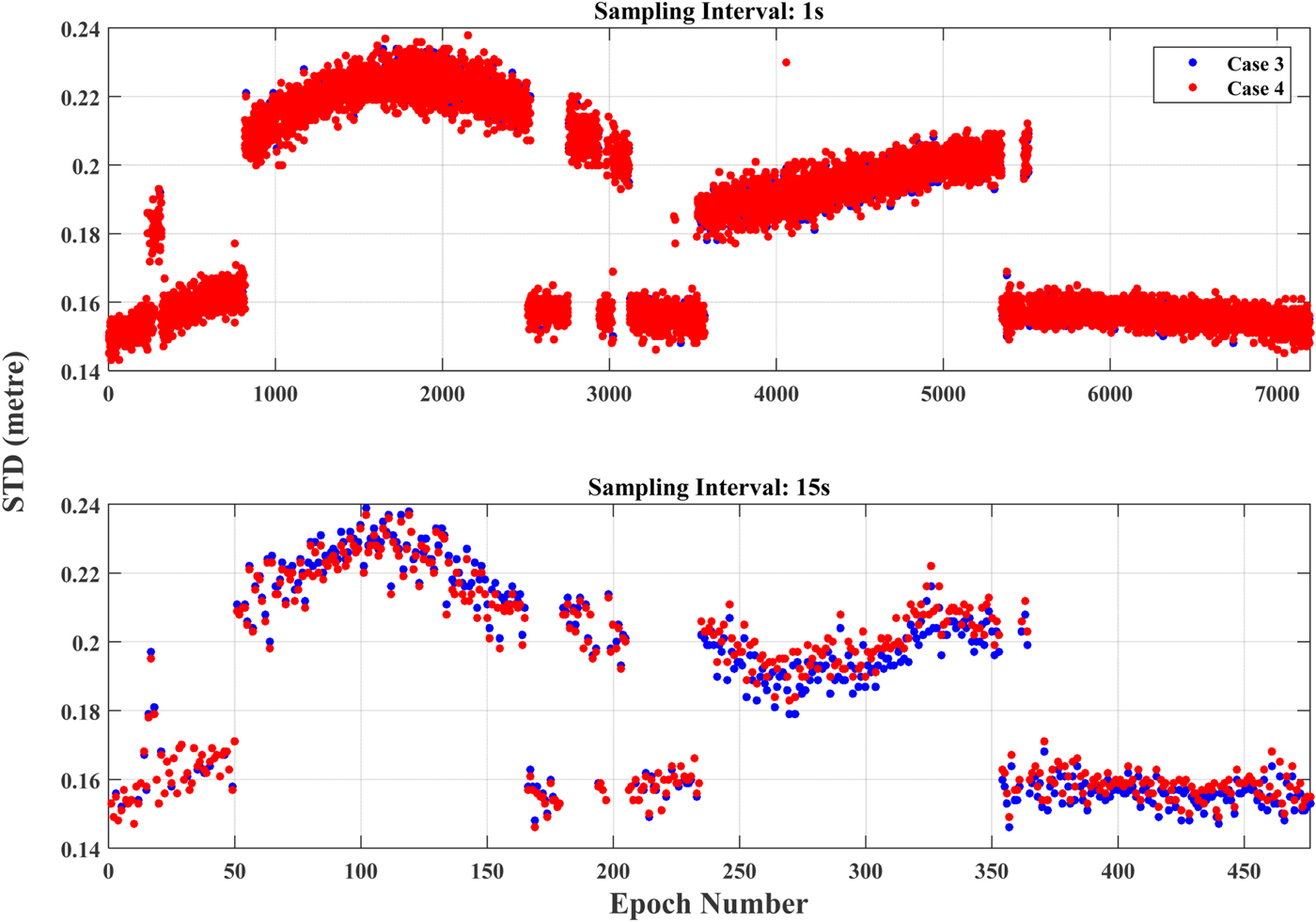
Figure 8. STD values with artificially added cycle slips of Case 3 (blue points) and Case 4 (red points).
It can be seen that all the cycle slips can be successfully detected with the threshold 0·05 m. The STD values of Case 4 are just slightly larger than those of Case 3, which demonstrates that the atmospheric errors, especially the ionospheric error, play a major role in the performance of this method since the use of precise orbit and clock products from the IGS has remarkably improved the accuracy of the initial coordinates obtained by SPP.
The procedure of the cycle slip repair is the same as with the experiments above. Figure 9 exhibits the float residuals of all the satellites of Case 3 and Case 4. As shown in Table 3, even the linearization error impact of Case 3 and Case 4 is diminished by using IGS precise products; the success rates of Case 3 and Case 4 are lower than those of Case 1 and Case 2, respectively. The possible reason is that the multipath error, the difference residuals of atmospheric and orbit errors, the shortening of the observation session and bad satellite-receiver geometry lead to this method having a worse repair performance. In addition, the repair success rate of a half-cycle slip was slightly influenced by the linearization error ε when the sampling interval was 15 s. Therefore, only the one-cycle slip can be repaired in practical applications with a 15 s sampling interval.

Figure 9. Float residuals of all the satellites of Case 3 and Case 4. The red, green and blue points represent the float residual of PRN26, PRN10 and all the other satellites of Case 3, respectively. The grey points represent the float residuals of all the satellites of Case 4.
3.4. Kinematic experiment (Case 5)
The Case 2 and Case 4 experiments 4 can be regarded as simulated kinematic experiments by using static data since the initial coordinates are obtained with SPP epoch-by-epoch. However, the observation environment of static data is always better compared with real kinematic data. In this section, a real kinematic data set collected in a complete aerial triangulation operation is used for the analysis of the performance of this method. The data was collected from 02:13:39 to 08:23:09 on 4 October 2013 in Shijiazhuang of Hebei province of China by Wuhan University with the use of Hi-target GNSS receivers. The sampling rate is 1Hz and the flight track is displayed in Figure 10. The longest baseline can reach about 265 km while the shortest baseline is about 2·5 km. Thus, this kinematic data covers all the scenario of short (0–20 km), mid-length (20–50 km) and long baselines (>50 km).

Figure 10. Flight track.
After removing the epochs for the initialization of the processing software, there are 22,147 epochs of observation for cycle slip detection and repair. It should be noted that no cycle slip was artificially added into the raw data in this experiment. The performance of the method is demonstrated by the detection and repair for the cycle slip inside the raw data.
Firstly, the Type 1 STD values mentioned in Section 2 are calculated and displayed in Figure 11 with the baseline length and the number of satellites in common-view.

Figure 11. STD values with baseline lengths and the number of satellites in common-view.
It is quite obvious that the fluctuation of the STD value has a strong relationship with the number of satellites. However, it is hard to see the correlation between STD and baseline length, and this conclusion coincides with the discussion in Sections 3.1 to 3.3 that the effect of linearization error and atmospheric error can be neglected while using high-frequency data such as 1 Hz. Indeed, some cycle slips exist in the raw data since the STD values of 36 epochs are larger than the threshold 0·05 m. Thus, all the epochs with STD values larger than 0·05 m were picked up to do the cycle slip repair work. The Type 1 and Type 2 STD values of these 36 epochs are calculated and displayed in Figure 12, and the float residuals of all the satellites are displayed in Figure 13.

Figure 12. Type 1 (red points) and Type 2 (blue points) STD values of the 36 epochs.

Figure 13. Float residuals of all the satellites of the 36 epochs with cycle slips. The red points represent the possible half-cycle slips and the blue points represent the normal float residuals.
In Figure 12, the STD values are significantly decreased after the cycle slips are removed. The red points in Figure 13 can be numerically regarded as a half-cycle slip, but it is difficult to repair them based on the discussion above. In addition, it is also difficult to say all the cycle slips have been detected and repaired since the STD values have a strong correlation with the satellite geometry, and in some cases, the epoch with just one half-cycle slip cannot be detected by using the threshold 0·05 m, and this needs further research.
4. CONCLUSION
In this paper, we proposed a new method of cycle slip detection and repair based on the total differential of ambiguity and least squares adjustment for single-frequency data processing. Different thresholds are used for STD, and detection and repair of integer and half-cycle slips.
To validate this method, experiments with static data of short and long baselines were firstly carried out. It was found that for short baselines with high accuracy initial coordinates, the success rate of cycle slip detection and repair can reach 100%, while if low accuracy initial coordinates were used, 15 s was the maximum sampling interval for this method to repair half-cycle slips. For long baseline experiments, IGS final orbits and clocks were used to improve the accuracy of initial coordinates, which can mitigate the negative impact of initial coordinates. However, due to the non-negligible atmospheric effects, the sampling interval should be less than 15 s for correctly detecting and repairing half-cycle slips. At the same time, the detection and repair of one-cycle slip can still reach a 100% success rate.
A set of real kinematic data with no artificially added cycle slips was used to demonstrate the performance of this method for kinematic applications. This kinematic data covers all the scenarios of short (0–20 km), mid-length (20–50 km) and long baselines (>50 km). The results indicate that half-cycle slips exist in the real data and can be detected. However, it is difficult to detect all the cases of half-cycle slips by using the empirical threshold of 0·05 m and it also appears to be impossible to repair the half-cycle slips with a threshold of 0·05 cycles.
This method performs quite well in both cycle slip detection and repair with single frequency data, especially in the cases of frequent occurrences of cycle slips. However, it should be mentioned that the computational process of this method is relatively complex since the least square estimation is adopted to identify the satellites with no cycle slips and then detect and repair the cycle slip. If multiple cycle slips occur, this method becomes more time-consuming, which will affect the performance of this method for real-time applications, especially high kinematic real-time applications.
ACKNOWLEDGEMENTS
This work was supported by the National Natural Science Foundation of China (Grant No. 41525014, 41374033 and 41210006) and the Program for Changjiang Scholars of the Ministry of Education of China. The University of Nottingham and the China Scholarship Council are both thanked for their sponsorships awarded to the first author for him to study in the UK for one year. Dr Xiaolin Meng at the University of Nottingham, as the first author's PhD supervisor abroad, has made a lot of constructive suggestions about how to improve the quality of this manuscript. Miss Roxanne Parnham at the University of Nottingham helped with proofreading this paper.


