


I. INTRODUCTION
We have previously proposed a whole-pattern deconvolution method for laboratory powder X-ray diffraction data (Ida and Toraya, Reference Ida and Toraya2002). It may appear to be equivalent to a curve-fitting method with a peak profile model synthesized by multiple convolutions with instrumental functions, often referred as “fundamental-parameters approach” (FPA) (Cheary and Coelho, Reference Cheary and Coelho1992).
In theoretical and practical points of view, there are both favorable and unfavorable features in the deconvolution method. Since all the deconvolution treatment can be completed by application of the fast Fourier transform (FFT) algorithm, the computation time needed for deconvolution–convolution treatment is quite short. There is practically no restriction about the complexity about the spectroscopic profile model for the source X-ray to be assumed, as demonstrated in another article (Ida et al., Reference Ida2018). Deconvolution method can remove the deformation of peak profile caused by instrumental aberrations, and it will be helpful to find possible intrinsic asymmetry of diffraction peak profile, which may be caused by inhomogeneous strain, stacking fault, chemical inhomogeneity, etc. without any structure model or identification of phases.
The effects of spectroscopic profile and instrumental aberrations on the observed diffraction profile are not exactly expressed by the convolution with instrumental functions on the scale of diffraction angle 2θ, while the effect of the spectroscopic profile of source X-ray is exactly expressed by convolution on the scale of ln sinθ, for example. Application of appropriate scale transform can easily be implemented in the whole-pattern deconvolution–convolution method, while it is quite difficult to treat the 2θ-dependence of the instrumental function properly in the FPA method. The FPA method usually applies the instrumental function determined at the peak position to whole the diffraction peak profile, even if the tails of lower- and higher-angle sides of the peak should be affected by different instrumental functions when the observed peak is broad.
On the other hand, there is theoretical difficulty about the estimation of error propagation in the whole-pattern deconvolution–convolution method. Even if the statistical errors in the observed diffraction intensity data can be assumed to be statistically independent, the deconvolved–convolved data will lose the independence.
There was another problem in the method described in our previous report (Ida and Toraya, Reference Ida and Toraya2002), where the effects of axial-divergence aberration were modeled by the convolution of two component functions defined on the transformed scale of abscissa,  $\chi ^{\prime}_ - = - \ln \cos \theta $ and
  $\chi ^{\prime}_ + = \ln \sin \theta $ for the diffraction angle 2θ.
The model could simulate primary dependence of the axial-divergence aberration upon the diffraction angle, where the broadenings of the lower- and higher-angle components are proportional to  $\cot \theta $ and tanθ, respectively. However, detailed cumulant analysis on the theoretical formula of axial-divergence aberration function suggests that there is a small discrepancy between the precise formula for the axial-divergence aberration and the convolution model applied in the previous whole-pattern deconvolution treatment. In this study, the mathematical formula for the convolution model for axial-divergence aberration has been modified to meet the requirements that the lower-order cumulants of the approximate formula should have the same values as the precise formula.
II. THEORETICAL
A. Characteristics of the axial-divergence aberration function
The axial-divergence aberration function ω A(Δ2θ) for a powder diffractometer with Bragg–Brentano geometry is well approximated by the following integral formula (Ida, Reference Ida1998):
 $$\eqalign{\omega _{\rm A} \left( {\Delta 2\theta} \right) = &\displaystyle{1 \over {{\rm \Psi} ^2}} \int \limits_{ - {\rm \Psi}} ^{\rm \Psi} \int \limits_{ - {\rm \Psi}} ^{\rm \Psi} \left( {1 - \displaystyle{{\left \vert \alpha \right \vert} \over {\rm \Psi}}} \right)\left( {1 - \displaystyle{{\left \vert \beta \right \vert} \over {\rm \Psi}}} \right) \cr &\times {\rm \delta} \left( {\Delta 2\theta + \displaystyle{{\left( {\alpha - \beta} \right)^2} \over {4\tan \theta}} - \displaystyle{{\left( {\alpha + \beta} \right)^2 \tan \theta} \over 4}} \right){\rm d}\alpha {\rm d}\beta, \;} $$
where Ψ is the axial-divergence angle defined by the ratio of the interval to the length of the Soller slits, 2θ is the diffraction angle, and δ(x) is the Dirac delta function. The characteristics of the axial-divergence aberration function ω A(Δ2θ) can be derived without solving Eq. (1) (see Appendix A).
The average position 2θ A of the function ω A(2θ) is given by
 $$2\theta _{\rm A} \equiv \int \limits_{ - \infty} ^\infty x\omega _{\rm A} \left( x \right){\rm d}x = \displaystyle{{{\rm \Psi} ^2} \over {12}}\left( {\tan \theta - \cot \theta} \right),\; $$
and the variance  $\left( {{\rm \Delta} 2\theta} \right)^2 _{\rm A} $, which can be connected with the peak width, is given by
 $$\left( {{\rm \Delta} 2\theta} \right)^2 _{\rm A} = \displaystyle{{17{\rm \Psi} ^4} \over {1440}}\left( {\tan ^2 \theta + \displaystyle{6 \over {17}} + \cot ^2 \theta} \right).\; $$
 The third-order central moment  $\left( {{\rm \Delta} 2\theta} \right)^3 _{\rm A} $, which can be connected with the asymmetry in peak shape, is given by
 $$\left( {{\rm \Delta} 2\theta} \right)^3 _{\rm A} = \displaystyle{{169{\rm \Psi} ^6} \over {60480}}\left( {\tan ^3 \theta + \displaystyle{{81\tan \theta} \over {169}}} \right.\; \left. { - \displaystyle{{81\cot \theta} \over {169}} - \cot ^3 \theta} \right),\; $$
The average, variance, and third-order central moment are identical to the first, second, and third-order cumulants of the function ω A(Δ2θ), respectively. Note that the formula previously proposed (Ida and Toraya, Reference Ida and Toraya2002) could only model the third-order central moment proportional to  $\left( {\tan ^3 \theta - \cot ^3 \theta} \right)$.
Since the cumulant of the convolution is generally equal to the sum of cumulants of component functions, it should not be very difficult to construct an approximate convolution formula that can reproduce exact values of both the first and third-order cumulants of the function ω A(2θ).
It is assumed that there is no need to change the effects of the even-order cumulants of the instrumental function on the deconvolution–convolution treatment.
B. Scale transform of convolution model for axial-divergence aberration
We have noticed that slight modification of the formula for the scale transform allows us to achieve coincidence of both the first and third-order cumulants of the axial-divergence aberration function with the convolution of two asymmetric functions defined on two different scales of abscissa.
The formulas of two abscissa scales, χ + and χ −, which should be used on the deconvolution–convolution treatment instead of the diffraction angle 2θ, are given by the following equation:
 $$\chi _ \pm = \pm \displaystyle{{\ln \left[ {1 + \beta \mp \left( {1 - \beta} \right)\cos 2\theta} \right]} \over {1 - \beta}} \;, $$
where β is a constant given by
 $$\beta = \displaystyle{{71 - 14\sqrt {22}} \over {27}} = 0.197562.$$
The derivation of the above formulas and the constant value of β in Eq. (6) is described in Appendix B.
C. Model component functions
A model for the component functions examined in this study is an extension of that used in our previous study (Ida and Toraya, Reference Ida and Toraya2002), modified to reproduce the shift (first-order cumulant) and asymmetric shape (third-order cumulant) of the axial-divergence aberration function. The formula for the component functions w ±(χ ±) defined on the scales of χ ± is given by
 $$w_ \pm \left( {\chi _ \pm} \right) = w\left( { \pm \chi _ \pm} \right),$$
 $$w\left( \chi \right) = \left\{ {\matrix{ {\displaystyle{1 \over {{\rm \Gamma} \left( \alpha \right)\gamma}} \left( {\displaystyle{{\chi - \delta} \over \gamma}} \right)^{\alpha - 1} \exp \left( { - \displaystyle{{\chi - \delta} \over \gamma}} \right)} & {\left[ {\delta \lt \chi} \right]} \cr 0 & {\left[ {\chi \le \delta} \right],} \cr}} \right.$$
where δ and γ are given by
 $$\delta = \displaystyle{{{\rm \Psi} ^2} \over {12\left( {1 - \beta} \right)}} - \alpha \gamma, \; $$
 $$\gamma = \left[ {\displaystyle{{169} \over {120960\alpha \left( {1 - \beta ^3} \right)}}} \right]^{1/3} {\rm \Psi} ^2 {\rm \;}. $$
The function Γ(α) in Eq. (8) is the gamma function defined by
 $${\rm \Gamma} \left( \alpha \right) \equiv \int \limits_0^\infty t^{\alpha - 1} {\rm e}^{ - t} {\rm d}t . $$
The details about the derivation of the above formulas are described in Appendix C.
The analytical formula of the Fourier transform of the function w(χ) is given by
 $$W\left( \xi \right) \equiv \int \limits_{ - \infty} ^\infty w\left( \chi \right){\rm e}^{2{\rm \pi i}\xi \chi} {\rm d}\chi = \displaystyle{{{\rm e}^{2{\rm \pi i}\xi \delta}} \over {\left( {1 - 2{\rm \pi i}\xi \gamma} \right)^\alpha}} {\rm \;}. $$
The first- and third-order cumulants of the convolution of the component functions on 2θ-scale are then both coincided with those of the axial-divergence aberration function described in Section II.A. The second-order cumulant of the convolution model given by
 $$\left( {{\rm \Delta} 2\theta} \right)^2 = \alpha \gamma ^2 \left( {1 + \beta ^2} \right)\left( {\tan ^2 \theta + \displaystyle{{54} \over {71}} + \cot ^2 \theta} \right){\rm \;} $$
is different from that given in Eq. (3), but the difference does not matter in the treatment applied in the method proposed in this paper, as will be shown in Section II.D.
D. Deconvolution–convolution treatment of axial-divergence aberration
Deconvolution–convolution treatment of axial-divergence aberration is divided into two steps, treatments on two abscissa scales, χ + and χ −, given in Eq. (5).
When the observed powder diffraction intensity data are given as a set of diffraction angles and intensities (2θ, I), the abscissa and ordinate values are changed to (χ ±, η ±), where the transformation of the intensity values are given by
 $$\eta _ + = IC\left( {2\theta} \right)\left( {\tan \theta + \beta {\rm cot}\; \theta} \right) , $$
 $$\eta _ - = IC\left( {2\theta} \right)\left( {\cot \theta + \beta {\rm tan}\; \theta} \right). $$
The function C(2θ) in Eqs. (14) and (15) is the geometric correction factor given by
 $$C\left( {2\theta} \right) = \displaystyle{{2\sin \theta \sin 2\theta} \over {1 + \cos ^2 2\theta}} $$
for a Bragg–Brentano powder diffractometer without a diffractive optical element.
The deconvolution–convolution process about intensities,  $\left( {\eta _ \pm } \right)_j \to \left( {\eta ^{\prime}_ \pm } \right)_j $, applied here is expressed by
 $$\left( {\eta ^{\prime}_ \pm} \right)_j = \displaystyle{1 \over n}\mathop \sum \limits_{k = - n/2}^{n/2} \displaystyle{{\left \vert {W_ \pm \left( {\xi _k} \right)} \right \vert} \over {W_ \pm \left( {\xi _k} \right)}}I_k \exp \left( { - \displaystyle{{2{\rm \pi i}kj} \over n}} \right)\;, $$
 $$\xi _k = \displaystyle{k \over {n\Delta \chi _ \pm}} \;, $$
 $$I_k = \mathop \sum \limits_{\,j = 0}^{n - 1} \left( {\eta _ \pm} \right)_j \exp \left( {\displaystyle{{2\pi ikj} \over n}} \right)\;, $$
where Δχ ± is the sampling interval on the χ ± scale. Multiplication by |W ±(ξ k)| on division by W ±(ξ k) in Eq. (17) confirms that the effects of even-order cumulants of the instrumental function are unchanged by the treatment (see Appendix D), even if the used model function does not precisely reproduce the even-order cumulants of the instrumental function. This treatment is equivalent to the convolution of a symmetrized instrumental function on deconvolution with an asymmetric instrumental function.
We have already suggested that this treatment can effectively smoothen the deconvolved intensity profile (Ida and Hibino, Reference Ida and Hibino2006), but it is rather essential to the current method, because the second-order cumulants of the convolution of the model functions are clearly different from that of the exact instrumental function, as shown in Eqs. (3) and (13). Note that the line-broadening effect of the axial divergence aberration still remains in the deconvolved–convolved data, and the effect should be modeled by the formula given in Eq. (3), if necessary.
E. Error propagation in deconvolution–convolution process
Even if the statistical errors in the observed intensity data can be assumed to be mutually independent, the errors in the deconvolved data will lose the independence on the deconvolution process. In other words, the error (covariance) matrix of the deconvolved data should have non-zero off-diagonal elements. In our previous report (Ida and Toraya, Reference Ida and Toraya2002), we have suggested two types of simplification to evaluate the errors in deconvolved data: (i) neglect of the off-diagonals elements of the covariance matrix and (ii) neglect of the off-diagonal elements of the weight matrix, which is identical to the inverse matrix of the covariance matrix.
The analytical results based on the former simplification assuming counting statistical errors have shown an overestimation of errors in low-intensity reflections, and those based on the latter simplification have shown an underestimation of errors in high-intensity reflections (Ida and Toraya, Reference Ida and Toraya2002). As it is currently well known that powder diffraction data are also affected by other types of statistical errors (Ida et al., Reference Ida, Goto and Hibino2009), we can apply the latter simplification as the more appropriate treatment of the errors in the deconvolved data almost in no doubt.
The statistical variance in the deconvolved data are then evaluated as the reciprocal of the correlation of the reciprocal of the source variance with the squared instrumental function (Ida and Toraya, Reference Ida and Toraya2002). The treatment may appear to refuse zero-count data, but a Bayesian interpretation (see Appendix E) or use of calculated intensity instead of the observed count (Antoniadis et al., Reference Antoniadis, Berruyer and Filhol1990) will solve the problem.
III. ANALYSIS OF EXPERIMENTAL DATA
A. Experimental
Powder diffraction data of standard LaB6 powder (NIST SRM660a) were collected with a powder diffraction measurement system (PANalytical, X'Pert PRO MTD) of θ–θ-type goniometer equipped with a micoro-focus Cu-target sealed tube with the effective focal width of W S = 0.04 mm operated at 45 kV and 40 mA, and a one-dimensional Si strip detector (PANalytical X'Celerator) at the distance of R = 240 mm from the rotation axis of the goniometer. The interval of the detector strips was W D = 0.075 mm. The 2Θ-margins of the X-ray source Δ2ΘS and the detector Δ2ΘD are estimated at
 $$\Delta 2{\rm \Theta} _{\rm S} = \displaystyle{{180^\circ} \over \pi} \displaystyle{{0.04} \over {240}} = 0.0095^\circ, $$
 $$\Delta 2{\rm \Theta} _{\rm D} = \displaystyle{{180^\circ} \over \pi} \displaystyle{{0.075} \over {240}} = 0.0179^\circ, $$
and the standard statistical error in the diffraction angle, Δ2θ, is then estimated at
 $$\Delta 2\theta = \sqrt {\displaystyle{{\left( {\Delta 2{\rm \Theta} _{\rm S}} \right)^2 \;+\; \left( {\Delta 2{\rm \Theta} _{\rm D}} \right)^2} \over {12}}} = 0.0059^\circ, $$
on the assumption of uniform probability distribution about the detection of X-ray photons.
Fixed-angle divergence slit of 0.5° and a couple of Soller slits with the open angle of 0.04 rad were used. Ni foil of 0.02 mm in thickness was used as a Kβ filter. The one-dimensional powder diffraction intensity data were created by an automatic measurement/data-processing program (PANalytical, Data Collector) from the integration of five iterations of continuous scans for the diffraction angles ranging from 10° to 145° with the nominal step interval of 0.0167° and nominal measurement time of 10.16 s step−1. Further details about the experimental conditions are described elsewhere (Ida et al., submitted).
B. Optimization of the component functions
The optimum values of the shape parameter α in the model component functions were searched by fitting the Pearson VII peak profile function with the linear background to the deconvolved intensities around observed LaB6 100-reflection. The Pearson VII function with the integral breadth of B is given by
 $$f_{{\rm P}7} \left( {k;B,\mu} \right) = \displaystyle{1 \over B}\left\{ {1 + \pi \left[ {\displaystyle{{{\rm \Gamma} \left( {\mu - 1/2} \right)k} \over {{\rm \Gamma} \left( \mu \right)B}}} \right]^2} \right\}^{ - \mu} \;, $$
where μ is a shape parameter. The Pearson VII function becomes identical to the Gaussian function for the limit μ → ∞, modified Lorentizan, intermediate Lorentzian, and Lorentzian for μ = 2, 1.5, and 1, respectively, and the profile will become “super-Lorentzian” for 0.5 < μ < 1 (Ida, Reference Ida2008). The values of χ 2 of the fitting, defined by
 $$\chi ^2 = \mathop \sum \limits_{\,j = 0}^{n - 1} \displaystyle{1 \over {\sigma _j^2}} \left[ {y_j - f\left( {x_j} \right)} \right]^2 \;, $$
have been evaluated for α = 0.02, 0.04, …, 0.98, where {y j} is the deconvolved data, f(x j) is the value of the Pearson VII function, and {σ j} is the estimated error in the deconvolved data, initially assumed to be the propagation of the counting statistical error and the 2θ-error propagation to intensity in the source data (Ida, Reference Ida2016). The reason why the 2θ-error propagation is taken into account in the current analysis is explained in Appendix F.
The effects of the spectroscopic intensity distribution of the source X-ray have been removed by the deconvolution–convolution method described in another article (Ida et al., Reference Ida, Ono, Hattan, Yoshida, Takatsu and Nomura2018). The asymmetric deformation and peak-shift caused by the flat-specimen and sample-transparency aberrations have also been removed by the method previously proposed (Ida and Toraya, Reference Ida and Toraya2002).
Figure 1 shows the dependence of minimum χ 2 on the variation of α, where the axial-divergence angle is assumed to be Ψ = 2.29° (0.04 rad). The value of χ 2 has a minimum about 141 at α = 0.80. The number of analyzed data points was N = 63 for the 100-reflection, and the number of adjusted parameters were P = 6. The larger value of χ 2 than (N–P) may be caused by the difference of the intrinsic peak profile from Pearson VII function or underestimation of statistical errors.

Figure 1. (Colour online) The values of χ2 evaluated for Pearson VII fitting to the deconvolved 100-peak profile on variation of the parameter α.
The results of Pearson VII curve fitting to the deconvolved–convolved LaB6 100-peak profile are shown in Figure 2(c) and (d). The shape parameter of the Pearson VII function is optimized to be μ = 1.00(14), which indicates that the profile of the deconvolved–convolved data are close to the Lorentizan profile.

Figure 2. (Colour online) (a) Observed LaB6 100-reflection data and an FPA fitting curve calculated by a combination of pseudo-Voigt functions (Thompson et al., Reference Thompson, Cox and Hastings1987) with a fixed Lorentzian components (Deutsch et al., Reference Deutsch, Förster, Hölzer, Hartwig, Hämäläinen, Kao, Huotari and Diamant2004), and multiply convolved with the instrumental aberration functions (Ida and Kimura, Reference Ida and Kimura1999a; Reference Ida and Kimurab), (b) estimated errors and fitting residuals in (a), (c) deconvolved–convolved data and the optimized symmetric Pearson VII function, and (d) estimated errors and fitting residuals in (c). Vertical arrows in (a) and (c) indicate the peak locations estimated by the FPA analysis and deconvolution–convolution treatment.
The residuals of the Pearson VII fitting for the deconvolved–convolved 100-reflection shows six-node profile (six crossing points to the zero line) as can be seen in Figure 2(d), which confirms that the intensity, peak location, width, asymmetry, and sharpness of the peak profile are reproduced by the optimized Pearson VII function. Since the apparently larger deviation from the assumed error is almost systematic, it does not mean the underestimation of errors, but rather indicates the mismatch of the Pearson VII fitting. If the systematic part of the deviation can be removed, the residuals (statistical errors) might be close to or even smaller than the assumed errors. It is concluded that there is no evidence that indicates overestimation or underestimation of errors, even though the error estimation applied here might be quite different from a traditional way.
It is also likely that the deviation is partly affected by the particle statistics (Ida and Izumi, Reference Ida and Izumi2011, Reference Ida and Izumi2013). The estimation of unknown errors should be based on a maximum-likelihood approach, but we here apply a simplified method just to avoid possible underestimation of errors in optimized profile parameters. The method is based on least-squares minimization to the squared residuals  $\left\{ {r_j^2} \right\}$ by the sum of statistical variance assuming the following formula:
 $$r_j^2 \approx \sigma _j^2 + f\left( {y_{{\rm obs}}} \right)_j^2 \;, $$
where f is an adjustable parameter, σ j is the initially estimated error, and (y obs)j is the observed intensity. The second term on the right-hand side of Eq. (25) can approximately be corresponded to the effects of particle statistics. The error values adjusted by Eq. (25) are also shown in Figure 2(d). The results of the final Pearson VII fitting shown in Figures 2(c) and 2(d) are based on the errors adjusted by the above method, but no significant difference from the results based on the initially assumed errors has been detected. The assumed errors might be overestimated, but the effect of particle statistics should be less significant on the scan with one-dimensional detector, because the integration of the intensities from the different detector strips should enhance the probability that a randomly oriented crystallite satisfies the diffraction condition, and increase the number of diffracting crystallites that contributes to the observed diffraction intensities.
C. Comparison with convolved (FPA) profile fitting to observed data
The observed diffraction data are analyzed by individual profile fitting with an FPA model, which is a diffraction peak profile model synthesized by combination of the pseudo-Voigt function (Thompson et al., Reference Thompson, Cox and Hastings1987), CuKα emission profile (Deutsch et al., Reference Deutsch, Förster, Hölzer, Hartwig, Hämäläinen, Kao, Huotari and Diamant2004), and approximate instrumental aberration functions (Ida and Kimura, Reference Ida and Kimura1999a; Reference Ida and Kimurab). All instrumental parameters including 11 independent parameters to determine four Lorentzian components of the normalized CuKα emission profile, axial divergence angle Ψ, equatorial divergence angle Φ, penetration depth μ −1, and goniometer radius R were treated as fixed constants. The formula used for the fitting is given by the following equations:
 $$f\left( {2\theta} \right) = b_0 + b_1 \left( {2\theta - 2\theta _1} \right) + If_{{\rm S*A*F*T}} \left( {2\theta - 2\theta _1} \right)\;, $$
 $$f_{{\rm S*A*F*T}} \left( {\Delta 2\theta} \right) = f_{\rm S} \left( {\Delta 2\theta} \right)*\omega _{\rm A} \left( {\Delta 2\theta} \right)*\omega _{\rm F} \left( {\Delta 2\theta} \right)*\omega _{\rm T} \left( {\Delta 2\theta} \right)\;, $$
 $$f_{\rm S} \left( {\Delta 2\theta} \right) = f_{{\rm TCH}} \left( {\Delta 2\theta ;\; W_{\rm G}, W_{\rm L}} \right)*f_\alpha \left( {\Delta 2\theta} \right)\;, $$
where b 0 and b 1 are background parameters, 2θ 1 is the nominal Kα 1 peak position, I is the integrated intensity, and the function f S*A*F*T(2θ) is the multiple convolution of the function f S(Δ2θ) with the approximate instrumental aberration functions for axial-divergence ω A(Δ2θ) (Ida, Reference Ida1998), flat-specimen ω F(Δ2θ) (Ida and Kimura, Reference Ida and Kimura1999a), and sample transparency ω T(Δ2θ) (Ida and Kimura, Reference Ida and Kimura1999b). The function f S(Δ2θ) is the convolution of the pseudo-Voight function f TCH(Δ2θ; W G, W L) determined by the full-width at half-maximum (FWHM) of the Gaussian and Lorentzian components, W G and W L (Thompson et al., Reference Thompson, Cox and Hastings1987), with the CuKα emission profile f α(Δ2θ) (Deutsch et al., Reference Deutsch, Förster, Hölzer, Hartwig, Hämäläinen, Kao, Huotari and Diamant2004). Two background parameters, intensity, peak position, and Gaussian and Lorentzian width, {b 0, b 1, I, 2θ 1, W G, W L}, are treated as adjustable parameters.
The results of the FPA fitting to LaB6 100-reflection are shown in Figures 2(a) and 2(b). The amount of errors estimated for the observed data and the errors caused by counting statistics are also shown in Figure 2(b). Most part of the errors estimated for the 100-peak is assigned to the propagation of 2θ-errors, and the results of fitting suggest overestimation of errors. It is not surprising, because the sensitivity of the strip detector should not be uniform, and the effective width of a strip detector is likely to be more restricted than the interval of the strips.
The optimized values of Kα 1-peak location, marked by vertical arrows in Figures 2(a) and 2(c), are 2θ 100 = 21.3672(11)° and 21.36561(12)° for the observed and deconvolved–convolved data, respectively. There is slight discrepancy between the above values of 2θ 100 beyond the estimated errors, but the apparent peak profile of the source data and the estimated peak positions in Figures 2(a) and 2(c) support that the deconvolution–convolution treatment automatically corrects the apparent peak shift caused by instrumental aberrations, similarly to the FPA-fitting method.
The optimized value of the FWHM of the Gaussian component of the FPA fit to the 100-reflection, W G = 0.003(12)°, may appear to be consistent with that the deconvolved–convolved 100-reflection data also show Lorentzian-like profile with the optimized Pearson VII shape parameter of μ = 1.000(14), but the relation is not straightforward, because the deconvolved–convolved data are not intrinsic diffraction peak profile, but the convolution with the symmetrized instrumental functions.
Figures 2(b) and 2(d) show a remarkable reduction of the estimated statistical errors through the deconvolution–convolution process. A tendency to underestimation of errors may be introduced by the neglect of the off-diagonal elements of the weight matrix on the deconvolution–convolution process, but the difference plot shown in Figure 2(d) still supports that the calculated errors are not heavily underestimated.
Figures 3 and 4 show the analytical results for 321 and 510-reflections. The FPA fitting for 510-refection shows significant deviation from the observed data, but it should not be caused by possible faults of the assumed spectroscopic or instrumental parameters because the deconvolved–convolved data based on the same parameters do not show such significant deviation. The discrepancy in the results of FPA analysis is likely to be caused by the insufficient implementation of the model applied here.
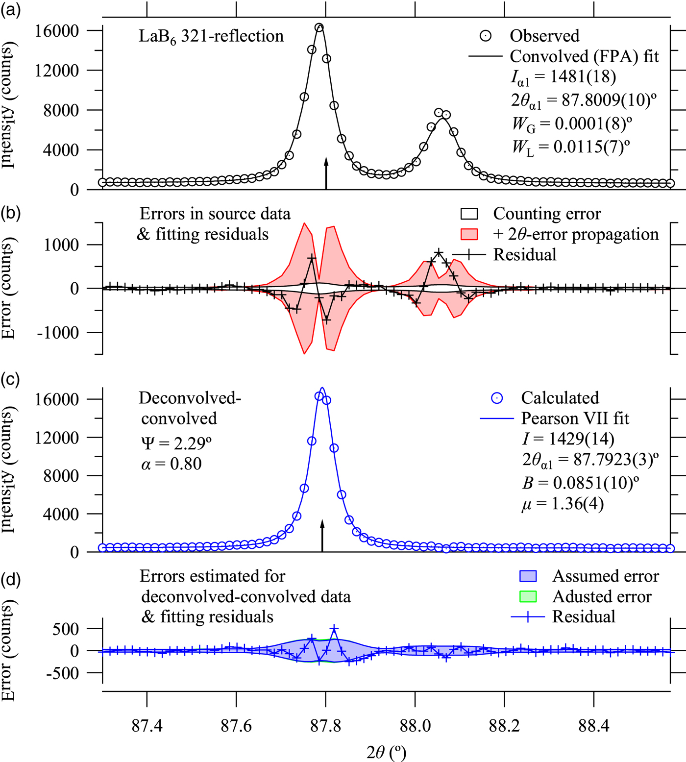
Figure 3. (Colour online) Observed data, fitting results to the observed data, deconvolved–convolved data, and fitting results to the deconvolved–convolved data about LaB6 321-reflection. See the caption of Figure 2 for the definitions.
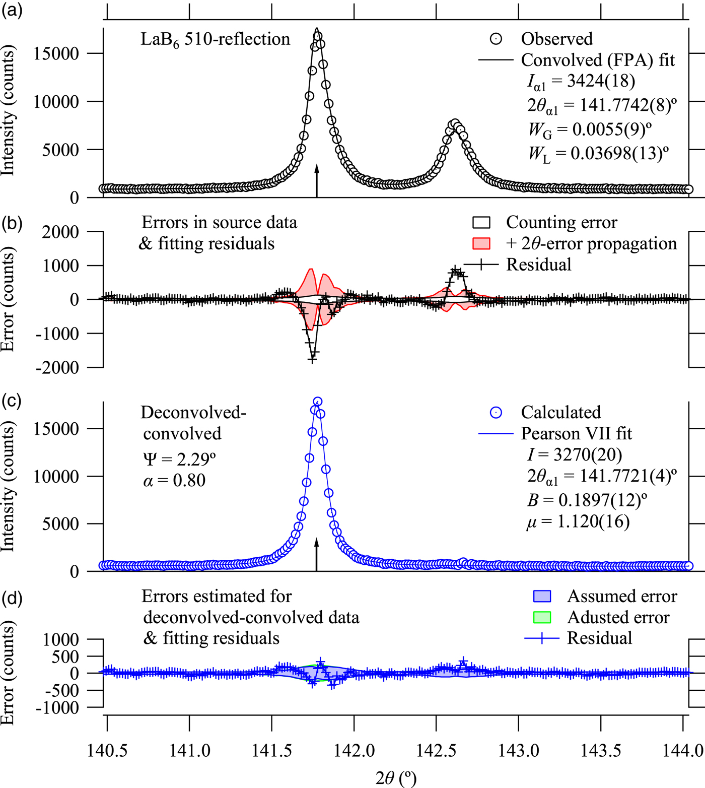
Figure 4. (Colour online) Observed data, fitting results to the observed data, deconvolved–convolved data, and fitting results to the deconvolved–convolved data about LaB6 510-reflection. See the caption of Figure 2 for the definitions.
D. Peak positions
The effects of automatic peak-shift correction expected to be achieved by both the FPA and deconvolution–convolution methods have been examined by evaluating the nominal lattice parameter a hkl calculated from each peak position 2θ hkl, by the following equation:
 $$a_{hkl} = \displaystyle{{\lambda _{\alpha 1} \sqrt {h^2 + k^2 + l^2}} \over {2\sin \theta _{hkl}}}, $$
where λ α1 = 1.5405929 Å is the assumed CuKα 1 peak wavelength. The values of a hkl calculated for 23 peak locations are plotted in Figure 5.

Figure 5. (Colour online) (a) Nominal lattice constants calculated from the 2θ peak positions evaluated by FPA analysis, and fitting curves calculated by a naive model, and (b) estimated errors and fitting residuals in (a), (c) Nominal lattice constants from deconvolution–convoution treatments, fitting curves calculated by naive and modified models, and (d) estimated errors and residuals of the modified fitting model.
Firstly, a naive model for the peak shift (McCusker et al., Reference McCusker, Von Dreele, Cox, Loër and Scardi1999) was applied, the formula of which to simulate the calculated lattice constant a hkl is given by
 $$a_{hkl} = \displaystyle{{a_{{\rm true}} \sin \theta ^{\prime}_{hkl}} \over {\sin \theta _{hkl}}}, $$
 $$2\theta ^{\prime}_{hkl} = 2\theta _{hkl} - {\rm \Delta} 2{\rm \Theta} _0 + \displaystyle{{2{\rm \Delta S}\cos \theta _{hkl}} \over R},$$
where a true is the true lattice constant of LaB6, Δ2Θ0 the constant error about the diffraction angle (zero offset), ΔS the displacement of the sample face from the rotation axis of the goniometer, and R is the goniometer radius. The errors in the calculated lattice constants, Δa hkl, were estimated by the difference of the values calculated for 2θ hkl and 2θ hkl + Δ2θ hkl, where Δ2θ hkl is the error in 2θ hkl evaluated by the profile fitting as the propagation of the assumed errors in the intensity data.
The results for the values estimated by the FPA analysis are well reproduced by the naive model, and systematic deviation is not clear, as shown in Figures 5(a) and 5(b). It should be noted that no significant trend to suggest overestimation of errors in the estimated peak positions has been detected in Figure 5(b).
In contrast, the values estimated by the Pearson VII fitting to the deconvolved–convolved data are clearly deviated from the optimized naive model, as can be seen in Figure 5(c).
It is suggested that additional peak shift has artificially been introduced on the deconvolution–convolution treatment applying the approximate formula for the axial-divergence aberration. The naive model given by Eq. (31) is then replaced by a modified formula given by
 $$2\theta ^{\prime}_{hkl} = 2\theta _{hkl} - {\rm \Delta} 2{\rm \Theta} _0 + \displaystyle{{2{\rm \Delta S}\cos \theta _{hkl}} \over R}$$
 $$\quad\quad\quad - {\rm \Delta} 2{\rm \Theta} _1 \left( {\tan \theta _{hkl} - \cot \theta _{hkl}} \right),$$
where Δ2Θ1 is an additional adjustable parameter.
The modified model given by Eq. (32) certainly improves the fitting to the dependence of a hkl on 2θ, as can be seen in Figure 5(c), and the additional parameter Δ2Θ1 has been optimized to be 0.00122(5)°. No systematic behavior of the residuals of the modified fitting is detected in the difference plot in Figure 5(d), and the values of residuals appear to be consistent with the estimated statistical errors.
Since the addition of the term in Eq. (32) is just a slight modification of the shift parameter used in the deconvolution–convolution calculation about the axial-divergence aberration, δ in Eq. (8), the adjustment of the shift can be easily implemented. The deconvolution–convolution treatment is then retried, just after replacing the shift parameter δ defined in Eq. (9) by δ′, given by
 $$\delta ^{\prime} = \delta - \displaystyle{{{\rm \Delta} 2{\rm \Theta} _1} \over {1 - \beta}} \;. $$
The nominal lattice constants calculated from the data treated by the deconvolution–convolution method incorporating the shift adjustment are shown in Figure 6. The apparent dependence on the diffraction angle is now reproduced by the naive model given by Eq. (31), as expected. The value of zero-offset error Δ2Θ0 estimated at 0.0006(4)°, and the sample displacement error ΔS estimated at −0.0017(8) mm are both acceptable values. The value of lattice constant a true is estimated at 4.156911(5) Å, while the certified value of NIST SRM660a is 4.156916(10) Å at 22.5 °C. The true lattice constant a true should be corresponded to the extrapolated value of a hkl to the limit of 2θ hkl → 180° in the naive model for the peak shift, as can be seen in Figures 5 and 6, and it is generally difficult to certify the validity of extrapolation. Precise temperature control and repeated experiments with refilled powder sample should be required for more detailed discussions of accuracy or precision about the estimation of lattice constants. However, the results of FPA analysis shown in Figure 5(a) suggest that insufficient implementation of the FPA model might cause systematic deviation of the estimated peak positions and hence the systematic error on the evaluation of the lattice dimensions.

Figure 6. (Colour online) (a) Nominal lattice constants calculated after the shift adjustment on deconvolution–convolution process and fitting curve based on a naive model, and (b) estimated errors and fitting residuals.
E. Peak shape
The optimized values of peak shape parameter μ of the Pearson VII peak profile function defined by Eq. (23) are plotted in Figure 7. The dependence of the shape parameter μ on 2θ shows maximum (minimum sharpness) at about 2θ ≈ 70°, and the sharpness of the peak shape increases on both sides of lower and higher diffraction angles. It should naturally be caused by increasing contribution of the effects of sharp axial-divergence aberration function for 2θ → 0° and 2θ → 180°. Furthermore, the dependence also suggests that μ approaches 1/2 at both the limits 2θ → 0° and 2θ → 180°, where both the Pearson VII function and the axial-divergence aberration function would become singular. The asymmetry of the dependence on 2θ is also reasonable because the contribution of the spectral width of the source X-ray, modeled by a Lorentzian function similarly increases on the higher-angle side and the relative contribution of the axial-divergence function should be reduced as compared with that on the lower-angle side.

Figure 7. (Colour online) Pearson VII shape parameter μ optimized by individual profile fitting to the deconvolved–convolved data (circles), and a cubic fitting curve (broken line).
The dependence of μ on 2θ is then modeled by a cubic curve given by
 $$\mu = \displaystyle{1 \over 2} + \left( {2\theta - 2\theta _0} \right)\left( {2\theta _1 - 2\theta} \right)\left( {\mu _0 + \mu _1 2\theta} \right),$$
for the fixed values (2θ 0, 2θ 1) = (0°, 180°). The adjustable parameters (μ 0, μ 1) are optimized at [1.64(2) × 10−4, 5.2(2) × 10−7 (°)−1].
F. Integral breadth
The optimized values of the integral breadth B of the Pearson VII peak profile function defined by Eq. (23) are plotted in Figure 8. As the deconvolved–convolved peak profile is close to the Lorentzian profile, the integral breadth is modeled by
 $$B = B_0 \tan \theta + B_1 + B_2 \cot \theta , $$
where B 0, B 1, and B 2 are adjustable parameters. The optimized values are B 0 = 0.0543(5)°, B 1 = 0.02331(7)°, and B 2 = 0.011113(2)°.

Figure 8. (Colour online) Integral breadth B optimized by individual profile fitting to the deconvolved–convolved data and a fitting curve.
Since the CuKα 1 FWHM is assumed to be 2.29 eV against the peak position 8047.83 eV (Ida et al., Reference Ida, Ono, Hattan, Yoshida, Takatsu and Nomura2018), the contribution of the spectral width to the coefficient B 0 is estimated at 0.051° as the integral breadth. As the interval of the Si detector strips and the effective width of the line-focus X-ray source are nominally 0.075 and 0.04 mm, the angular resolution for the goniometer radius of 240 mm is estimated at 0.0059° as the standard deviation, which can be related to the value estimated for the constant term B 1 in Eq. (35). The coefficients of tanθ and  $\cot \theta $-terms of the broadening caused by axial-divergence aberration for Ψ = 2.29° should be corresponded to
  $\sqrt {17/1440} {\rm \Psi} ^2 = 0.010^ \circ $ as the standard deviation, and the constant term in the axial-divergence aberration should be
  ${\rm \Psi} ^2 /\sqrt {240} = 0.006^ \circ $ as the standard deviation, as given in Eq. (3). The broadening caused by flat-specimen aberration should also be proportional to
  $\cot \theta $, but the effect is considered to be negligible in this case, because the coefficient is corresponded to
  ${\rm \Phi} ^2 /\sqrt {45} = 0.0007^ \circ $ as the standard deviation for the equatorial open angle of Φ = 0.5°.
G. Whole-pattern fitting
A whole-pattern fitting method known as the Pawley method (Pawley Reference Pawley1981) has been applied to the overall deconvolved–convolved data. Ninth-order polynomial of 2θ has been used for background intensity and the symmetric Pearson VII function is used as the peak profile function, the intensities of which are calculated in the range of ten times of integral breadth around the peak position. The overall intensities are modeled by the following equation:
 $$y_j = \mathop \sum \limits_{n = 0}^9 b_n \left( {2\theta _j} \right)^n + \mathop \sum \limits_{\,p = 0}^{22} I_p f_{{\rm P}7} \left( {2\theta _j - 2\theta _p ;B\left( {2\theta _p} \right),\mu \left( {2\theta _p} \right)} \right)\; \;, $$
where the background parameters {b n}, peak intensities {I p}, lattice constant, zero-offset, and sample displacement, {a true, Δ2Θ0, ΔS} to determine the peak positions 2θ p, and the width parameters {B 0, B 1, B 2} defined in Eq. (35), and shape parameters {μ 0, μ 1} in Eq. (34) are treated as adjustable parameters. The least-squares fitting assuming the propagation of the counting errors and 2θ-error propagation have been applied.
The values of optimized parameters are listed in Tables I and II. Figure 9 shows the result of whole pattern fitting. The R values are estimated at R p = 4.43% and R wp = 5.32%, and the goodness-of-fit parameter at S = 1.34.

Figure 9. (Colour online) Results of whole pattern fitting to the deconvolved–convolved data.
Table I. Integrated intensities of CuKα 1 components evaluated by individual FPA profile fitting to source data (IPF-FPA/S), Pearson VII fitting to deconvolved–convolved data (IPF-P7/DC), and whole-pattern fitting to deconvolved–convolved data (WPF-P7/DC).

Table II. Lattice constant, peak shift, and profile parameters evaluated by individual FPA fitting to source data (IPF-FPA/S), individual Pearson VII fitting to deconvolved–convolved data (IPF-P7/DC), and whole-pattern fitting to deconvolved–convolved data (WPF-P7/DC).

IV. CONCLUSION
An improved formula to simulate the effects of axial-divergence aberration in Bragg–Brentano geometry has been developed. Deformation of observed powder diffraction peak profile caused by axial-divergence aberration can effectively be removed by a deconvolution–convolution method based on the mathematical model. The powder diffraction peak profile of LaB6 treated by the method has well been reproduced by a symmetric Pearson VII function. The peak positions of the deconvolved–convolved data can be simulated by a naive model about the possible zero-offset error and the displacement of the sample face. The overall peak profile in the deconvolved–convolved data have been modeled by three parameters to determine the integral breadth (width) and two parameters to determine the shape (sharpness), and the optimized values of the width-parameters are reasonably corresponded to the instrumental constants.
Appendix A Calculation of cumulants of axial-divergence aberration function
The nth-order cumulant κ n of a function w(x) is generally defined by the following equation:
 $$\kappa _n = \mathop {\lim} \limits_{\theta \to 0} \left[ {\displaystyle{{\partial ^n} \over {\partial \theta ^n}} \ln \int \limits_{ - \infty} ^\infty {\rm e}^{\theta x} w\left( x \right){\rm d}x} \right]\;.$$
When w(x) is a normalized function, the first-order cumulant:
 $$\kappa _1 = \int \limits_{ - \infty} ^\infty xw\left( x \right){\rm d}x$$
is identical to the average x, the second-order cumulant:
 $$\kappa _2 = \langle x^2 \rangle- \langle x\rangle^2 \;$$
is identical to the variance 〈(x − 〈x〉)2〉, and the third-order cumulant:
 $$\kappa _3 =\langle x^3 \rangle - 3\langle x^2\rangle \langle x \rangle + 2\langle x \rangle^3 \;$$
is identical to the third-order central moment 〈(x − 〈x〉)3〉. Higher-order cumulants are also expressed by the combination of the average of nth power of x, 〈x n〉.
When the instrumental function is expressed by the following formula:
 $$w\left( x \right) = \int \limits_{\alpha _{{\rm min}}} ^{\alpha _{{\rm max}}} {\rm \delta} \left( {x - g\left( \alpha \right)} \right)f\left( \alpha \right){\rm d}\alpha \;,$$
the average of nth power of x is calculated by
 $$\langle x^n \rangle= \int \limits_{ - \infty} ^\infty x^n w\left( x \right){\rm d}x = \int \limits_{\alpha _{{\rm min}}} ^{\alpha _{{\rm max}}} \left[ {g\left( \alpha \right)} \right]^n f\left( \alpha \right){\rm d}\alpha \;.$$
Appendix B Derivation of scale transforms for axial-divergence aberration function
The basic idea of constructing the scale-transform formulas for a convolution model is not far from the one previously proposed (Ida and Toraya, Reference Ida and Toraya2002), where the scale transforms of  $\chi ^{\prime}_ + = \ln \sin \theta $ for the upper component and
  $\chi ^{\prime}_ - = - \ln \cos \theta $ for the lower component were applied. Since
  $\Delta 2\theta /\Delta \chi ^{\prime}_ + \propto \tan \theta $ and
  $\Delta 2\theta /\Delta \chi ^{\prime}_ - \propto {\rm cot}\theta $, the first and third-order cumulants of the convolution
  $w\left( {\chi ^{\prime}_ + } \right)*w\left( { - \chi ^{\prime}_ - } \right)$ should be proportional to
  $\left( {\tan \theta - \cot \theta} \right)$ and
  $\left( {\tan ^3 \theta - \cot ^3 \theta} \right)$, respectively.
The formula in Eq. (5) is derived as a solution of the following relations:
 $$\displaystyle{{\Delta 2\theta} \over {\Delta \chi _ +}} \propto \tan \theta + \beta {\rm cot}\; \theta,$$
 $$\displaystyle{{\Delta 2\theta} \over {\Delta \chi _ -}} \propto \cot \theta + \beta {\rm tan}\; \theta.$$
 Then the dependence of the third-order cumulant of the convolution model [w(χ + )*w( − χ − )] on the diffraction angle 2θ should be given by  $\left( {\tan \theta + \beta {\rm cot}\; \theta} \right)^3 - \left( {\cot \theta + \beta {\rm tan}\; \theta} \right)^3 $. The dependence on 2θ becomes proportional to the third-order cumulant of the axial-divergence aberration function given in Eq. (4), when the following equation is satisfied:
 $$\displaystyle{{3\beta} \over {1 + \beta + \beta ^2}} = \displaystyle{{81} \over {169}}\;.$$
The value of β given in Eq. (6) is the solution of Eq. (B3). Even if the numerical value of the coefficient β estimated at 0.197562 is not large, it is expected that addition of this term improves the approximation than the previous formula (Ida and Toraya, Reference Ida and Toraya2002), as is supported by the coincidence of the third-order cumulant with the precise formula. The coincidence of the first-order cumulant (average) can be achieved by the constant shift of the component function, described in Appendix C.
Appendix C Adjustment of the formula of component functions
It is assumed that the component functions of a convolution model are given by
 $$w_ \pm \left( {\chi _ \pm} \right) = \displaystyle{1 \over \gamma} g\left( {\displaystyle{{ \pm \chi _ \pm - \delta} \over \gamma}} \right)\;,$$
where g(x) is a normalized function. When the first, second and third-order cumulants of the function g(x) is given by 〈x〉, 〈(Δx)2〉 and 〈(Δx)3〉, respectively, the cumulants of the function w ±(χ ±) are given by
 $$\langle\chi _ \pm\rangle = \pm \gamma \left( {\langle x \rangle + \delta} \right),$$
 $$\langle\left( {{\rm \Delta} \chi _ \pm} \right)^2\rangle = \gamma ^2 \langle\left( {{\rm \Delta} x} \right)^2 \rangle{\rm \;},$$
 $$\langle\left( {{\rm \Delta} \chi _ \pm} \right)^3\rangle = \pm \gamma ^3 \langle\left( {{\rm \Delta} x} \right)^3\rangle {\rm \;},$$
and the cumulants of the convolution of the component functions on the 2θ–scale should be given by
 $$\langle2\theta\rangle = \gamma \left( {\langle x \rangle + \delta} \right)\left( {1 - \beta} \right)\left( {\tan \theta - \cot \theta} \right),$$
 $$\eqalign{\langle\left( {{\rm \Delta} 2\theta} \right)^2 \rangle &= \gamma ^2 \langle\left( {{\rm \Delta} x} \right)^2\rangle \left( {1 + \beta ^2} \right) \cr &\quad \times \left( {\tan ^2 \theta + \displaystyle{{4\beta} \over {1 + \beta ^2}} + \cot ^2 \theta} \right){\rm \;}},$$
 $$\eqalign{\langle\left( {{\rm \Delta} 2\theta} \right)^3 \rangle &= \gamma ^3 \langle\left( {{\rm \Delta} x} \right)^3 \rangle\left( {1 - \beta ^3} \right) \cr &\quad \times \left( {\tan ^3 \theta + \displaystyle{{3\beta \tan \theta} \over {1 + \beta + \beta ^2}}} \right.{\rm \;} \left. { - \displaystyle{{3\beta \cot \theta} \over {1 + \beta + \beta ^2}} - \cot ^3 \theta} \right).}$$
The parameter γ is adjusted by the relation in Eq. (C7) for the given values of  $\langle\left( {{\rm \Delta} 2\theta} \right)^3 _{\rm A} \rangle$, 〈(Δx)3〉 and β, and the parameter δ is then adjusted by the relation in Eq. (C5) for the given values of 2θ A, x, β, and γ.
The first and third-order cumulants of the model function w(χ) applied here are given by 〈χ〉 = αγ + δ and 〈(Δχ)3〉 = 2αγ 3, and the value of γ given in Eq. (21) is the solution of the equation:
 $$\displaystyle{{169{\rm \Psi} ^6} \over {60480}} = 2\alpha \gamma ^3 \left( {1 - \beta ^3} \right){\rm \;},$$
and the value of δ in Eq. (20) has been determined by the equation:
 $$\displaystyle{{{\rm \Psi} ^2} \over {12}} = {\rm \;} \left( {\alpha \gamma + \delta} \right)\left( {1 - \beta} \right),{\rm \;}$$
Appendix D Invariance of even-order cumulants on the deconvolution–convolution process
Absolute values of cumulants of functions f(x) and f(−x) are equal, and the signal is unchanged for even-order and inverted for odd-order cumulants. The autocorrelation of the function f(x), we here express by |f|2(x), is identical to the convolution of f(x) and f(−x). Since cumulants are additive on convolution, even-order cumulants of |f|2(x) become double of those of the function f(x), and odd number cumulants of |f|2(x) are zero. When we define a function |f|(x) by
 $$\left \vert f \right \vert \left( x \right) \equiv \int \limits_{ - \infty} ^\infty \left \vert {F\left( k \right)} \right \vert {\rm \; e}^{ - 2{\rm \pi i}kx} {\rm d}k,{\rm \;}$$
 $$F\left( k \right) \equiv \int \limits_{ - \infty} ^\infty f\left( x \right)\; e^{2{\rm \pi i}kx} {\rm d}x,\;$$
it is clear that the convolution of |f|(x) with itself is identical to the autocorrelation |f|2(x). Then even-order cumulants of |f|(x) are equal to those of f(x), and odd-order cumulants of |f|(x) are zero. We can confirm that the deconvolution with f(x) and convolution with |f|(x) only changes the odd-order cumulants, but keeps even-order cumulants, including integrated intensity (zeroth-order cumulant), variance (second-order cumulant), kurtosis (excess or sharpness; fourth-order cumulant) unchanged.
Appendix E Bayesian interpretation of zero-count data
When we assume uniform prior probability distribution for the intensity y,
 $$P\left( y \right) = \left\{ {\matrix{ {1/\varepsilon} & {\left[ {0 \lt y \lt \varepsilon} \right]} \cr 0 & {\left[ {{\rm elsewhere}} \right]} \cr}} \right.{\rm \;}, {\rm \;}$$
for an arbitrary large value of ε, and the likelihood function P(n|y) of Poisson distribution for the observed count n,
 $$P\left( {n \vert y} \right) = \displaystyle{{y^n {\rm e}^{ - y}} \over {n!}}{\rm \;}, {\rm \;}$$
the probability for n counts P(n) is given by
 $$P\left( n \right) = \int \limits_{ - \infty} ^\infty P\left( {n \vert y} \right)P\left( y \right){\rm d}y{\rm \;} $$
 $$= \displaystyle{1 \over \varepsilon} \mathop {\lim} \limits_{\varepsilon \to \infty} \int \limits_0^\varepsilon \displaystyle{{y^n {\rm e}^{ - y}} \over {n!}}{\rm d}y = \displaystyle{1 \over \varepsilon} \;.$$
Bayesian inference derives the posterior probability distribution from the observed count n given by
 $$P\left( {y \vert n} \right) = \displaystyle{{P\left( {n \vert y} \right)P\left( y \right)} \over {P\left( n \right)}} = \displaystyle{{y^n {\rm e}^{ - y}} \over {n!}}\;. {\rm \;}$$
The posterior probability for zero count is given by P(y|0) = e−y, and the expected values of average and variance are then both unity.
Appendix F Propagation of error in 2θ
It seems that most of the analyses about powder X-ray diffraction data are based on the assumption that the observed diffraction intensity I can be connected with a certain value of the theoretical diffraction angle 2θ. However, the size of the detector element is finite, no matter which type of a detector, a zero-dimensional, one-dimensional, or two-dimensional detector is used.
Figure 10 illustrates why it is considered to be necessary to take into account the errors in the goniometer angle 2Θ or the diffraction angle 2θ, the latter of which may be provided from a data acquisition system to users, to achieve statistical analysis of the observed diffraction intensity data.
If the center of a detector element of Δ2θ in width is located at the position of 2θ, it will detect the X-ray photons diffracted at the angles ranging from 2θ − Δ2θ/2 to 2θ + Δ2θ/2. It is expected that the detected intensities range from I − ΔI/2 to I + ΔI/2.

Figure 10. (Colour online) Schematic illustration to show the reason why the propagation of the error in the diffraction angle 2θ should be taken into account in the statistical analysis of the powder X-ray diffraction intensities.


