


1. Introduction
Coupling between electric fields  $\tilde {\boldsymbol {E}}$ and hydrodynamics – electrohydrodynamics (EHD) – has interested scientists since Gilbert reported that static electricity generated from rubbed amber could ‘attract’ water (Gilbert Reference Gilbert1958). The birth of the modern science of EHD, however, can be traced to three papers: Rayleigh's discovery (Rayleigh Reference Rayleigh1882; Tsamopoulos, Akylas & Brown Reference Tsamopoulos, Akylas and Brown1985) that highly charged drops can become unstable, Taylor's analysis (Taylor Reference Taylor1964) of equilibria and stability of conducting drops subjected to
  $\tilde {\boldsymbol {E}}$ that showed that strong fields can deform drops into prolate shapes with conical tips along
  $\tilde {\boldsymbol {E}}$ (Miksis Reference Miksis1981; Basaran & Scriven Reference Basaran and Scriven1990), and Taylor's discovery (Taylor Reference Taylor1966) that imperfectly conducting or leaky dielectric (LD) (Melcher & Taylor Reference Melcher and Taylor1969) drops can be deformed parallel (prolate) or perpendicular (oblate) to
  $\tilde {\boldsymbol {E}}$. These papers and experiments (Zeleny Reference Zeleny1917) on jet emission or EHD tipstreaming (Collins et al. Reference Collins, Jones, Harris and Basaran2008, Reference Collins, Sambath, Harris and Basaran2013; Oddershede & Nagel Reference Oddershede and Nagel2000; Burton & Taborek Reference Burton and Taborek2011) from the conical ends of pendant drops – electrospraying (Barrero & Loscertales Reference Barrero and Loscertales2007; Fernández de La Mora Reference Fernández de La Mora2007; Ganán-Calvo et al. Reference Ganán-Calvo, López-Herrera, Herrada, Ramos and Montanero2018) – laid the foundation for widely used applications. Examples – all involving highly conducting drops surrounded by a gas and prolate deformations – include electrospray ionization mass spectrometry, electrospinning, and printing of cells (Fenn et al. Reference Fenn, Mann, Meng, Wong and Whitehouse1989; Feng Reference Feng2002; Jayasinghe, Qureshi & Eagles Reference Jayasinghe, Qureshi and Eagles2006; Reneker & Yarin Reference Reneker and Yarin2008).
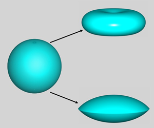
Cases where both phases are viscous fluids (Marín et al. Reference Marín, Loscertales, Marquez and Barrero2007; Vlahovska Reference Vlahovska2019) and drops exhibit both prolate and oblate deformations have been receiving increasing attention (Feng & Scott Reference Feng and Scott1996; Lac & Homsy Reference Lac and Homsy2007; Yariv & Rhodes Reference Yariv and Rhodes2013; Das & Saintillan Reference Das and Saintillan2017a,Reference Das and Saintillanb) due to their wide-ranging importance (Harris, Sisson & Basaran Reference Harris, Sisson and Basaran1992; Zhang, Basaran & Wham Reference Zhang, Basaran and Wham1995; Baygents, Rivette & Stone Reference Baygents, Rivette and Stone1998; Eow et al. Reference Eow, Ghadiri, Sharif and Williams2001; Marín et al. Reference Marín, Loscertales, Marquez and Barrero2007; Bird et al. Reference Bird, Ristenpart, Belmonte and Stone2009; Ristenpart et al. Reference Ristenpart, Bird, Belmonte, Dollar and Stone2009). Recent experiments (Brosseau & Vlahovska Reference Brosseau and Vlahovska2017) have uncovered a previously unknown type of EHD equatorial streaming instability. Here, a poorly conducting drop is dispersed in a more conducting exterior liquid (figure 1a). A weak  $\tilde {\boldsymbol {E}}$ drives the drop to adopt an oblate shape, in accord with theory (Taylor Reference Taylor1966; Melcher & Taylor Reference Melcher and Taylor1969). As shown in Brosseau & Vlahovska (Reference Brosseau and Vlahovska2017) and Vlahovska (Reference Vlahovska2019), such drops become unstable as
  $|\tilde {\boldsymbol {E}}|$ increases. Although it is known that the nature of the instabilities that arise with oblate drops depends on the ratio of fluid viscosities, the physical mechanisms for their onset have heretofore remained elusive and are uncovered from theory in this paper. We demonstrate that if the drop is more viscous, electric shear stress plays a dominant role and a strong
  $\tilde {\boldsymbol {E}}$ creates a dimple at each pole of the oblate drop that resembles a discocyte or biconcave disk (figure 1b). These dimples grow and the drop eventually ruptures to form a torus. This mode of breakup is called dimpling. If the exterior phase is more viscous, we show that a strong
  $\tilde {\boldsymbol {E}}$ drives the oblate drop into a biconvex lens (figure 1c) because equatorial normal stresses – electric, hydrodynamic and capillary – become unbounded as
  $|\tilde {\boldsymbol {E}}|$ increases. Interestingly, Torza, Cox & Mason (Reference Torza, Cox and Mason1971) have briefly mentioned in a couple of sentences the occurrence of lenses in their experiments, albeit without further discussion. In the recent experiments, rings of fluid are then emitted from the lens-shaped drop's equator which subsequently break into droplets (Brosseau & Vlahovska Reference Brosseau and Vlahovska2017; Vlahovska Reference Vlahovska2019). This mode of breakup is called equatorial streaming.

Figure 1.  $(a)$ A spherical drop subjected to an electric field. At large field strengths, the ratio of outer to inner fluid viscosity (
 $\mu _2/\mu _1$) determines the drop's fate:
  $(b)$ discocyte and
  $(c)$ lens. Here and in all of the figures that can be found in the remainder of this paper, all drop shapes that are shown are those that have been obtained from simulations.
We examine the physics for the onset of these two instabilities and their dependence on viscosity ratio by determining steady-state solutions of the governing equations by simulation. We adopt this approach as it is currently unclear whether dimpling and equatorial streaming instabilities arise due to the loss of stability of a steady-state solution at a turning (limit) point or a bifurcation point (Iooss & Joseph Reference Iooss and Joseph2012) with respect to applied field strength. We demonstrate that both instabilities arise at turning points when the applied field strength reaches a critical value. First, we take advantage of experimental results (Brosseau & Vlahovska Reference Brosseau and Vlahovska2017) to judiciously probe portions of the relevant parameter space that have been overlooked in previous computational studies (Feng & Scott Reference Feng and Scott1996; Feng Reference Feng1999; Lac & Homsy Reference Lac and Homsy2007). Second, contrary to some recent studies, we do not approximate solutions using expansions based on spheroidal harmonics (Bentenitis & Krause Reference Bentenitis and Krause2005; Zabarankin Reference Zabarankin2013). Lens-shaped drops have not been reported in these previous studies relying on the use of expansions based on spheroidal harmonics. Moreover, to date, when the exterior fluid is more viscous, only stable steady-states have been computed numerically (Zabarankin Reference Zabarankin2013; Lanauze, Walker & Khair Reference Lanauze, Walker and Khair2015). Hence, for the first time, we resolve theoretically the onset of the instability that arises when the exterior fluid is more viscous, in agreement with the equatorial streaming instability experimentally observed in Brosseau & Vlahovska (Reference Brosseau and Vlahovska2017).
The article is organized as follows. Section 2 describes the mathematical formulation of the problem. A brief summary of the numerical method used in the simulations is then provided in § 3. As it is imperative to impress upon the reader an intuitive understanding of drop deformation caused by an applied electric field, a quick overview is presented in § 4 on the physics of electric-field-induced deformation in drops of LD fluids as opposed to drops of perfectly conducting or perfectly insulating fluids. Simulation results are then presented and discussed in § 5. The paper concludes in § 6 with concluding remarks and a summary of possible directions for further study.
2. Problem statement
The system (figure 1) consists of two neutrally buoyant phases ( $i=1,2$;
  $i=1$, drop;
  $i=2$, exterior), each of which is an incompressible, Newtonian, LD (Melcher & Taylor Reference Melcher and Taylor1969; Saville Reference Saville1997) fluid of constant physical properties (viscosity
  $\mu _i$, permittivity
  $\epsilon _i$ and conductivity
  $\sigma _i$) undergoing Stokes flow. In the absence of electric field,
  ${\tilde {\boldsymbol {E}}}_i = \boldsymbol {0}$, the drop is a sphere of radius
  $R$. It bears no net charge. The interface separating the two fluids has constant surface tension
  $\gamma$ as well as diffusivity for charge
  $\mathcal {D}_s$. We use a cylindrical coordinate system
  $(\tilde {r}, \theta , \tilde {z})$ based at the centre of the sphere and where these variables stand for the radial, angular and axial coordinates. The drop is subjected to an electric field
  $\boldsymbol {\tilde {E}_0} = \tilde {E}_0\boldsymbol {e}_z$ of uniform strength
  $\tilde {E}_0$ far from the drop (
 $\boldsymbol {e}_z$: unit vector in
  $\tilde {z}$ direction). The problem is non-dimensionalized using as characteristic scales
  $R$ for length,
  $t_c \equiv \mu _1 R/\gamma$ for time (
 $t_c$: visco-capillary time),
  $\gamma /R$ for hydrodynamic stress,
  $\tilde {E}_0$ for electric field,
  $\epsilon _2 {\tilde {E}}_0$ for surface charge density and
  $\epsilon _2 \tilde {E}_0^2$ for electric stress. Aside from the three dimensionless parameter ratios
  $\chi \equiv \sigma _1/\sigma _2$,
  $\kappa \equiv \epsilon _1/\epsilon _2$ and
  $\lambda \equiv \mu _2/\mu _1$, three other dimensionless groups arise: (i) electric Bond number
  $N_E \equiv \epsilon _2\tilde {E}^2_0 R / 2 \gamma$ (the ratio of electric to surface tension force), (ii) dimensionless charge relaxation time in either phase,
  $\alpha _i\equiv (\epsilon _i/\sigma _i)/t_c$ (
 $i=1$ or
  $2$,
$2$,  $\alpha _2/\alpha _1 = \chi /\kappa$), and (iii) Péclet number
  $Pe\equiv (R^2/\mathcal {D}_s)/t_c = \gamma R/\mu _1 \mathcal {D}_s$ (the ratio of the time scale for charge diffusion on the surface
  $R^2/\mathcal {D}_s$ and the visco-capillary time
  $t_c$). In what follows, variables without tildes are the dimensionless counterparts of those with tildes.
The steady-state deformation of the drop and the flow field and electric potential  $\varPhi _i$ (where
  $\boldsymbol {E}_i = -\boldsymbol {\nabla }\varPhi _i$) inside (
 $\varOmega _1$) and outside (
 $\varOmega _2$) the drop are governed by the axisymmetric continuity, Stokes and Laplace equations:
 \begin{equation} \boldsymbol{\nabla} \boldsymbol{\cdot} \boldsymbol{v}_i = 0, \quad \boldsymbol{\nabla} \boldsymbol{\cdot} \boldsymbol{\mathsf{T}}^H_i=\boldsymbol{0}, \quad \nabla^2 \varPhi_i = 0 \quad \text{in}\ \varOmega_ i, \end{equation}
where  $\boldsymbol {v}_i$ is the velocity,
  $\boldsymbol{\mathsf{T}}^H_i \equiv -p_i\boldsymbol{\mathsf{I}} + (\mu _i/\mu _1)[(\boldsymbol {\nabla }\boldsymbol {v})_i + (\boldsymbol {\nabla }\boldsymbol {v})^T_i]$ the hydrodynamic stress, and
  $p_i$ the pressure.
Along the drop surface  $S_f$, the flow and electric field in each phase are coupled through the traction condition
 \begin{equation} \boldsymbol{n} \boldsymbol{\cdot} [\boldsymbol{\mathsf{T}}^H_i + 2N_E\boldsymbol{\mathsf{T}}^E_i]^2_1 =2\mathcal{H}\boldsymbol{n}, \end{equation}
where  $\boldsymbol{\mathsf{T}}^E_i \equiv ({\epsilon _i}/{\epsilon _2})(\boldsymbol {E}_i\boldsymbol {E}_i - E^2_i\boldsymbol{\mathsf{I}}/2)$ is the electric (Maxwell) stress tensor (Melcher & Taylor Reference Melcher and Taylor1969),
  $\boldsymbol {n}$ the outward-pointing unit normal and
  $2\mathcal {H}$ twice the mean curvature. The notation
  $[x]^2_1$ denotes the jump in
  $x$ in going from phase 1 to phase 2. Along
  $S_f$, the kinematic boundary condition
  $\boldsymbol {n} \boldsymbol {\cdot } \boldsymbol {v}_1 = \boldsymbol {n} \boldsymbol {\cdot } \boldsymbol {v}_2 = 0$ (Kistler & Scriven Reference Kistler, Scriven, Pearson and Richardson1983; Christodoulou & Scriven Reference Christodoulou and Scriven1992; Deen Reference Deen1998) and no slip
  $\boldsymbol {t} \boldsymbol {\cdot } [\boldsymbol {v}_i]^2_1=0$, where
  $\boldsymbol {t}$ denotes the unit tangent to
  $S_f$ in the cross-sectional plane, are imposed. Additionally along
  $S_f$, the tangential component of the electric field is continuous,
  $\boldsymbol {t} \boldsymbol {\cdot } [\boldsymbol {E}_i]^2_1=0$, but the normal component of the electric displacement suffers a discontinuity given by the surface charge density,
  $q \equiv \boldsymbol {n} \boldsymbol {\cdot } [(\epsilon _i/\epsilon _2)\boldsymbol {E}_i]^2_1$. In the LD model (Melcher & Taylor Reference Melcher and Taylor1969), bulk density of charge is zero but surface charge density on
  $S_f$ is governed by a transport equation which, under steady-state conditions, is given by
 \begin{equation} \boldsymbol{\nabla}_s \boldsymbol{\cdot} (q\boldsymbol{v}) - Pe^{-1} \nabla^2_s q = \frac {1}{\alpha_2} \left(\frac {\sigma_1}{\sigma_2} \boldsymbol{n} \boldsymbol{\cdot}\boldsymbol{E}_1 - \boldsymbol{n} \boldsymbol{\cdot} \boldsymbol{E}_2\right) \end{equation}
on  $S_f$. Here,
  $\boldsymbol {v}$ is the velocity and
  $\boldsymbol {E}_1$ and
  $\boldsymbol {E}_2$ are electric fields at
  $S_f$, and
  $\boldsymbol {\nabla }_s$ is the surface gradient. In this equation, the terms on the left side represent surface charge transport by convection and diffusion, and the source-like terms on the right represent charge transport from each phase to
  $S_f$ by Ohmic conduction. In the limit where charge transport by diffusion and charge transport by convection are negligible (Taylor Reference Taylor1966; Melcher & Taylor Reference Melcher and Taylor1969), this equation reduces to the continuity of the normal component of the electric current,
  $\boldsymbol {n} \boldsymbol {\cdot } [(\sigma _i/\sigma _2)\boldsymbol {E}_i]^2_1=0$.
3. Simulations and numerical method
The governing equations are solved by numerical simulation using a finite-element-based algorithm over one quadrant of the  $rz$-plane (
 $r$,
$r$,  $z\geq 0$) subject to symmetry conditions along
  $r=0$ (axis of symmetry) and
  $z=0$ (plane of symmetry). Far from the drop's centre-of-mass, the electric potential is set to asymptotically approach that of a uniform field and the flow field is taken to be stress-free. Similar versions of the algorithm employed here have been used for solving equilibrium (Basaran & Scriven Reference Basaran and Scriven1990; Sambath & Basaran Reference Sambath and Basaran2014), steady-state (Basaran & Scriven Reference Basaran and Scriven1988) and transient (Collins et al. Reference Collins, Sambath, Harris and Basaran2013) problems in EHD. The algorithm relies on elliptic mesh generation (Christodoulou & Scriven Reference Christodoulou and Scriven1992) and continuation with adaptive parameterization (Abbott Reference Abbott1978) to determine steady-state solution families (Feng & Basaran Reference Feng and Basaran1994), and automatically detects points where changes of stability occur (Brown & Scriven Reference Brown and Scriven1980; Ungar & Brown Reference Ungar and Brown1982; Yamaguchi, Chang & Brown Reference Yamaguchi, Chang and Brown1984). In all simulations,
  $Pe=10^3$ (Collins et al. Reference Collins, Jones, Harris and Basaran2008, Reference Collins, Sambath, Harris and Basaran2013). We note that all simulation results presented in the paper are insensitive to changes in
  $Pe$ provided that
  $Pe\gg 1$, as shown in the appendix.
4. Physics of drop deformation
Interfacial flows and drop deformations observed in LD fluids are made possible by the electric shear stress at  $S_f$,
  $[{\mathsf{T}}^E_{nt}]^2_1 \equiv \boldsymbol {n} \boldsymbol {\cdot } [\boldsymbol{\mathsf{T}}^E_i]^2_1 \boldsymbol {\cdot } \boldsymbol {t} = qE_t$ where
  $E_t \equiv \boldsymbol {t} \boldsymbol {\cdot } \boldsymbol {E}_i$. Following Taylor (Reference Taylor1966), we focus first on the situation in the absence of charge convection and diffusion. The electric normal stress at
  $S_f$ can then be expressed as
  $[{\mathsf{T}}^E_{nn}]^2_1 \equiv \boldsymbol {n} \boldsymbol {\cdot } [\boldsymbol{\mathsf{T}}^E_i]^2_1 \boldsymbol {\cdot } \boldsymbol {n} = [E_{1,n}^2 (\chi ^2 - \kappa ) + E_t^2 (\kappa -1)]/2$ where
  $E_{1,n} \equiv \boldsymbol {n} \boldsymbol {\cdot } \boldsymbol {E}_1$, and the charge density is given by
  $q=E_{1,n} (\chi - \kappa )$. When the drop has a smaller permittivity and is of relatively even lesser conductivity than the surrounding fluid,
  $\chi /\kappa = ({\epsilon _2}/{\sigma _2})({\sigma _1}/{\epsilon _1})<1$ and
  $\kappa = {\epsilon _1}/{\epsilon _2}<1$, electric normal stress
  $[{\mathsf{T}}^E_{nn}]^2_1$ is compressive, i.e. acts inward, but is not necessarily uniform, on
  $S_f$. Moreover, both
  $q$ and
  $[{\mathsf{T}}^E_{nt}]^2_1$ are negative (positive) on the top (bottom) half of the drop, and the flow along
  $S_f$ is therefore from the drop's poles to its equator.
We now illustrate that electric normal stress alone is insufficient to determine the drop's fate when the applied field is sufficiently weak so that a spherical drop suffers negligible deformation. If the drop were spherical, the field inside it would be uniform,  $\boldsymbol {E}_1={3\boldsymbol {e}_z}/({\chi +2})$. The electric normal stress at the poles is then given by
  $E_1^2(\chi ^2-\kappa )/2$, and that at the equator is
  $E_1^2(\kappa -1)/2$. When
  $\chi \to 0$, in this spherical state, it follows that the difference between the electric normal stress at the pole and at the equator,
  ${\rm \Delta} ^P_E([{\mathsf{T}}^E_{nn}]^2_1)$, is given by
  $E_1^2(-2\kappa + 1)/2$. Thus, if
  $\kappa = {\epsilon _1}/{\epsilon _2}>{1}/{2}$, then electric normal stress at the pole is more compressive than that at the equator
  $({\rm \Delta} ^P_E([{\mathsf{T}}^E_{nn}]^2_1)<0)$, and the converse is true for
  $\kappa < {1}/{2}$. If electric normal stress is more (less) compressive at the pole than at the equator, the drop is more likely to adopt an oblate (prolate) shape at finite field strengths. However, non-uniformity in electric normal stress is just one way of driving deformation in LD drops, whereas it is the sole way of doing so when the drop is either a perfect conductor or perfect insulator and the exterior a perfect insulator (Taylor Reference Taylor1964). A more exact analysis (Melcher & Taylor Reference Melcher and Taylor1969) including electric shear stress shows that when
  $\chi \to 0$ and
  $\lambda \to \infty$, transition between prolate and oblate deformations occurs at
  $\kappa = {5}/{16} = 0.3125$. Thus, as was first shown by Taylor (Reference Taylor1966) and Smith & Melcher (Reference Smith and Melcher1967), considering electric normal stress alone is in general insufficient, because it overlooks the role played by electric tangential and hydrodynamic normal stresses that may arise on account of flows induced by
  $[{\mathsf{T}}^E_{nt}]^2_1$.
To illustrate the crucial importance of electric shear stress, we examine next by simulations situations in which  ${\epsilon _1}/{\epsilon _2}={1}/{2}$ when
  $\chi \ll 1$ (as in the experiments of Brosseau & Vlahovska (Reference Brosseau and Vlahovska2017)). In this situation, electric normal stress is not only equal at the poles and the equator but is in fact uniform everywhere on the surface of a spherical drop. Since a uniform stress causes no deformation, the resulting drop deformation at low field strengths is driven by the action of electric shear stress. As the role of viscosity ratio in the dimpling and equatorial streaming instabilities has heretofore been incompletely understood, it is reasonable to anticipate that the goal of elucidating the mechanisms for the onset of these instabilities would be best accomplished by considering two limits in which the drop is either much more or much less viscous than the exterior fluid, viz.
  ${\mu _2}/{\mu _1}\ll 1$ or
  ${\mu _2}/{\mu _1}\gg 1$. In both limits, the direction of flow on
  $S_f$ does not change, as it is induced purely by electric shear stress, which depends solely on electrical properties.
5. Results and discussion
5.1. Limit of  $\mu _2/\mu _{1} \ll 1$

When  $\mu _2/\mu _1 \rightarrow 0$, the exterior fluid behaves as if it were a passive gas that simply exerts a constant pressure on the drop, and the physics can be appreciated by focusing on the flow in
  $\varOmega _1$. Here, electric tangential stress at
  $S_f$ drives fluid from the pole(s),
  $(r,z) = (0, \pm z|_{pole})$, to the equator,
  $(r,z)=(r|_{eq},0)$. Because of mass conservation, the pressure at the equator then has to rise compared to that at the pole(s) for the fluid to return to the pole(s). Thus, a recirculating eddy arises as shown in figure 2(a), and the resulting flow resembles those in the lid-driven cavity and Taylor pump (Melcher & Taylor Reference Melcher and Taylor1969; Basaran & Scriven Reference Basaran and Scriven1988). Because the pressure rises at the equator and falls at the poles, the curvature increases at the equator and decreases at the poles: the drop bulges out at the equator and flattens at the poles.

Figure 2. Steady-state streamlines  $(a)$ inside and
  $(b)$ outside, and pressure distributions inside/outside a drop in the limit of vanishingly small applied electric field strength for two systems in which the drop is much less conducting and has a lower permittivity than the exterior. Here and in the next two figures,
  $({\epsilon _2}/{\sigma _2})({\sigma _1}/{\epsilon _1})=0.02$,
  ${\epsilon _1}/{\epsilon _2}={1}/{2}$ and
  $\alpha _2=2 \times 10^{-4}$ (therefore,
  $\alpha _1=10^{-2}$). Panels (a) and (b) correspond, respectively, to the limits in which exterior viscosity and interior viscosity tend to zero. In both (a) and (b), warmer (cooler) or red (blue) colour implies higher (lower) pressure.
To better quantify drop deformation, figure 3(a) shows in a bifurcation diagram the variation of the steady-state deformation of the drop  $D\equiv (z|_{pole}-r|_{eq})/(z|_{pole}+r|_{eq})$ with electric Bond number
  $N_E$ for a system in which the drop is less conducting and has a lower permittivity but is much more viscous than the outer fluid. Figure 3(b) shows the variation with
  $D$ of the difference between the value at the pole and that at the equator of all three normal stresses. In order to better discern the role of electric normal stress
  $[{\mathsf{T}}^E_{nn}]^2_1$, two sets of solutions are shown in that figure: one set where electric normal stress in (2.2) is operative and another where this term has been turned off, i.e.
  $[{\mathsf{T}}^E_{nn}]^2_1=0$ (Collins et al. Reference Collins, Jones, Harris and Basaran2008; Kamat et al. Reference Kamat, Wagoner, Thete and Basaran2018). When electric normal stress is turned off, it can no longer induce and hence contribute to the deformation of the drop. By comparing solutions obtained when electric normal stress is acting and when it is absent, its role in determining the fate of the drop can be made plain.

Figure 3. Bifurcation diagram, stresses and drop shapes for steady-state solutions when the drop is much less conducting and has a lower permittivity but is much more viscous than the outer fluid ( ${\mu _2}/{\mu _1}= 0.02$). Variation of
  $(a)$ deformation
  $D$ with electric Bond number
  $N_E$ for shape families of dimpled shapes and
  $(b)$ difference between the value at the pole and the equator of all three normal stresses (hydrodynamic (red), electric (green), and capillary (blue)) with
  $D$. Solutions depicted in (a) and (b) here and in the next figure have been obtained from simulations in which electric normal stress
  $[{\mathsf{T}}_{nn}^E]_1^2$ is on (solid curves) and in its absence (dash-dotted curves). In panel
  $(a)$ here and in the next figure, circles indicate locations of turning points and shape insets show drop profiles when
  $[{\mathsf{T}}_{nn}^E]_1^2 = 0$ or
  $\ne 0$ at points marked by a square symbol.
  $(c)$ Sequence of drop shapes obtained from simulations along the shape family for which electric normal stress is turned off,
  $[{\mathsf{T}}_{nn}^E]_1^2=0$, and
  $(d)$ that for which this stress is operative,
  $[{\mathsf{T}}_{nn}^E]_1^2\neq 0$. In
  $(c)$, the values of
  $(N_E,D)$ for which these shapes are shown are
  $(0,0)$,
  $(0.583,-0.162)$,
  $(0.799,-0.431)$ and
  $(0.714,-0.626)$. In
  $(d)$, the values of
  $(N_E,D)$ for which these shapes are shown are
  $(0,0)$,
  $(0.581,-0.160)$,
  $(0.685,-0.429)$ and
  $(0.595,-0.625)$.
As can be seen in figure 3(b), electric tangential stress (as described earlier) causes hydrodynamic normal stress to rise at the equator and fall at the poles ( ${\rm \Delta} ^P_E([{\mathsf{T}}^H_{nn}]^2_1) < 0$). For small deformations (
 $|D|<0.2$), simulations with electric normal stress turned on show that there is virtually no electric normal stress difference between the pole and the equator. Hence, capillary normal stress (capillary pressure) must balance hydrodynamic normal stress (
 ${\rm \Delta} ^P_E(2\mathcal {H}) < 0$). As field strength or
  $N_E$ increases, electric shear stress and hence the concomitant flow strengthen, driving the hydrodynamic and capillary normal stresses to further rise at the equator and fall at the poles, and thereby to cause drop deformation to grow. This trend persists until the drop becomes flattened at the poles and the curvature there equals zero. Any further increase in electric shear stress and disparity in hydrodynamic normal stress between the equator and the pole(s) then causes the curvature at the pole(s) to change sign and hence causes a dimple(s) to form. Hence, we say that steady-state solutions that lie along either solution branch – with normal stress on and with it turned off – in the bifurcation diagram of figure 3(a) are members of the shape family (families) of dimpled shapes (discocytes). Figure 3(a) shows that as
  $N_E$ increases from zero, a turning point arises when
  $(N_E,D)=(N_E^*,D^*)$ along the solution families. It is shown in standard books on bifurcation theory (Glendinning Reference Glendinning1994; Seydel Reference Seydel2009; Iooss & Joseph Reference Iooss and Joseph2012) that starting with a solution that is known to be stable, solutions are linearly stable as a control parameter is varied until a turning point is reached. Here, the known stable solution corresponds to a spherical drop (
 $D=0$) in the absence of electric field or when the electrical Bond number
  $N_E$ – the control parameter – equals
  $0$. Therefore, as
  $N_E$ is increased, the solutions along a solution family or solution branch are stable until a turning point
  $(N_E^*,D^*)$ is reached. Whereas solutions for values of
  $0 < N_E^*$,
  $0 \le |D| < |D^*|$ are stable, those beyond the turning point(s) are unstable (Brown & Scriven Reference Brown and Scriven1980; Ungar & Brown Reference Ungar and Brown1982; Yamaguchi et al. Reference Yamaguchi, Chang and Brown1984; Feng & Basaran Reference Feng and Basaran1994; Glendinning Reference Glendinning1994; Seydel Reference Seydel2009; Iooss & Joseph Reference Iooss and Joseph2012). Comparison of the shape insets in figure 3(a) reveals that dimpling and instability occur even in the absence of electric normal stress and that electric normal stress acts to accentuate the dimple(s). Figure 3(a) further shows that the solution family with
  $[T_{nn}^E]_1^2$ turned on exhibits a second turning point as
  $|D|$ increases, a point that is returned to below. Sequences of drop shapes of increasing deformation along both shape families are shown in figures 3(c) and 3(d).
5.2. Limit of $\mu _2/\mu _{1} \gg 1$

When  $\mu _2/\mu _1 \rightarrow \infty$, the drop behaves like a void in which pressure is constant. In
  $\varOmega _2$, electric tangential stress on
  $S_f$ drives flow from the pole(s) to the equator just outside the drop. Thus, a pressure gradient arises along the symmetry axis where fluid far from the drop flows toward it such that pressure is low and normal viscous stress is compressive at the drop's pole(s),
  $(r,z)=(0,\pm z|_{pole})$, and a pressure gradient also arises at the plane of symmetry where fluid is driven from the equatorial mid-plane toward infinity such that pressure is high and normal viscous stress is extensional at the drop's equator,
  $(r,z)=(r|_{eq},0)$ (figure 2b). Unlike the dimpling case, here the pressure difference between the pole and equator causes a prolate drop deformation while the (larger) viscous normal stress difference drives an oblate deformation.
Figure 4(a) shows  $D$ as a function of
  $N_E$ for a system in which the drop is less conducting and has a lower permittivity but is also much less viscous than the outer fluid. Figure 4(b) shows the difference between the value at the pole and that at the equator of all three normal stresses as a function of
  $D$. Once again, solutions depicted in figure 4 have been obtained both with electric normal stress on and with it turned off. In the absence of electric normal stress,
  $[{\mathsf{T}}_{nn}^E]_1^2 = 0$, drop deformation is driven by hydrodynamic normal stress and balanced by capillary stress (figure 4b dash-dotted curves). In this case, the shape family reaches a turning point when
  $N_E \approx 1$: drops before the turning point are stable whereas those after it are unstable. However, the steady-state shapes (figure 4c) do not resemble the characteristic lens-like shapes that lead to equatorial streaming. This shape family is referred to as the family of spheroids. By contrast and as shown in figure 4(a), when
  $[{\mathsf{T}}_{nn}^E]_1^2 \ne 0$, electric normal stress acts to arrest the increase of
  $D$ with
  $N_E$. This is made plain by figure 4(b) which reveals that electric normal stress at the equator is more compressive than its counterpart(s) at the pole(s), thereby decreasing the extent of deformation. While deformation on the drop-scale (measured by
  $D$) is arrested, interface deformation at the local scale at the equator (measured by interface curvature or
  $|2\mathcal {H}|$) is enhanced. At the equator, under the action of ever increasing (normal) electric force, the three stresses comprising compressive electric normal stress, extensional hydrodynamic normal stress and capillary stress due to equatorial curvature not only compete but appear to grow without bound, giving rise to the solution family of lens-like shapes – the lens family – whose highly deformed members (figure 4d) are precursors to equatorial streaming. Thus, for the first time, we theoretically observe the onset of this instability (inset, figure 4a) in agreement with experimental results (Brosseau & Vlahovska Reference Brosseau and Vlahovska2017).

Figure 4. Same as figure 3 but where the drop is much less viscous than the outer fluid ( ${\mu _2}/{\mu _1}= 50$). Variation of
  $(a)$
$(a)$ $D$ with
  $N_E$ for shape families of spheroids (
 $[{\mathsf{T}}_{nn}^E]_1^2 = 0$) and lenses (
 $[{\mathsf{T}}_{nn}^E]_1^2 \ne 0$) and
  $(b)$ difference between the value at the pole and the equator of all three normal stresses (hydrodynamic (red), electric (green), and capillary (blue)) with
  $D$. The upper right inset in
  $(a)$ is a blow-up of the main figure where the turning point is located when
  $[{\mathsf{T}}_{nn}^E]_1^2 \ne 0$, i.e. the lens family. In the inset, values of
  $N_E$ are shown along the horizontal axis as in the main figure, but the vertical axis has been shifted so that the values shown correspond to
  $D + 0.444815$ for clarity.
  $(c)$ Sequence of drop shapes obtained from simulations along the family of spheroids (for which electric normal stress is turned off,
  $[{\mathsf{T}}_{nn}^E]_1^2=0$) and
  $(d)$ that for the lens family (for which this stress is operative,
  $[{\mathsf{T}}_{nn}^E]_1^2\neq 0$). In
  $(c)$, the values of
  $(N_E,D)$ for which these shapes are shown are
  $(0,0)$,
  $(0.731,-0.148)$,
  $(1.122,-0.374)$ and
  $(0.797,-0.608)$. In
  $(d)$, the values of
  $(N_E,D)$ for which these shapes are shown are
  $(0,0)$,
  $(0.774,-0.155)$,
  $(1.442,-0.382)$ and
  $(2.930,-0.445)$.
6. Conclusions
When the exterior fluid's conductivity is much larger than the drop's, members of shape families of drops become increasingly deformed as electric field strength or electric Bond number  $N_E$ rises and lose stability at turning points. Highly deformed members of these families are discocytes when the drop is much more viscous than its exterior,
  $\mu _2/\mu _1 \ll 1$, and lenses when
  $\mu _2/\mu _1 \gg 1$, in accord with experiments (Brosseau & Vlahovska Reference Brosseau and Vlahovska2017; Vlahovska Reference Vlahovska2019). Through careful scrutiny of the stresses acting to deform a drop, it has been conclusively shown that the instability that arises in the former case is caused by a drastically different mechanism than the latter one. It has been shown that dimpling occurs purely as a result of electric tangential stress: dimple-shaped drops arise and become unstable at a turning point in
  $N_E$ with and without electric normal stress. However, lens-shaped drops arise as a result of electric normal stress and do not occur in its absence. Theoretical analysis of the rim of the lens, similar to those in studies of the conic cusp singularity in EHD tipstreaming from the Taylor cones at the tips of prolate drops (Zubarev Reference Zubarev2001; Collins et al. Reference Collins, Jones, Harris and Basaran2008), is so far lacking, but is underway.
While the geometry of the lens and that of the Taylor cone is similar, the analogy between these two phenomena ends there. A Taylor cone (Taylor Reference Taylor1964) exists under electrohydrostatic conditions, i.e. in the absence of flow, in which electric and capillary normal stresses balance. Unlike Taylor cones, lenses form only in the presence of flow. Consequently, viscous, electric and capillary normal stresses are in balance in the case of lenses. Another crucial difference between the two cases is that in Taylor cones, electric and capillary normal stresses act in opposite directions at the apex of the cone, whereas in lenses they act in the same direction, i.e. they are compressional or act inward, at the equator.
It was heretofore unknown whether equatorial streaming could be predicted using the LD equations. It has been demonstrated here that these equations do give rise to unstable solutions. Once destabilized, lens-shaped drops emit equatorial sheets, as has been shown in a preliminary computational study in which the unstable steady-state shapes beyond the turning point along the lens family are used as initial conditions in transient simulations (Wagoner et al. Reference Wagoner, Anthony, Vlahovska, Harris and Basaran2019). Developing a thorough understanding of the transient dynamics that occurs when drops become unstable and succumb to dimpling ( $\mu _2/\mu _1 \ll 1$) or equatorial streaming (
 $\mu _2/\mu _1 \gg 1$) is of great theoretical importance and is underway. It is noteworthy that interface shapes in the vicinity of the axis of symmetry, i.e. near
  $r=0$, both above and below the plane of symmetry, appear conical for drops that are members of the family of dimpled shapes (discocytes). When these conical interfaces approach each other after the onset of the dimpling instability, the dynamics that ensues should follow that reported in Bird et al. (Reference Bird, Ristenpart, Belmonte and Stone2009). Thus, whether the cone angle is larger or smaller than the critical cone angle reported in Bird et al. (Reference Bird, Ristenpart, Belmonte and Stone2009) would determine whether the outcome is dimple merger or recoil. Investigating which of the two outcomes arises once a dimple-shaped drop has destabilized is left as an open problem for future computational studies on the transient dynamics of unstable discocytes.
According to the results presented in § 5.1, two turning points arise along the family of discocytes (figure 3). Thus, while there is a loss of stability at the first turning point, the family regains its stability at the second turning point (Glendinning Reference Glendinning1994; Seydel Reference Seydel2009). Hence, the family of discocytes exhibits hysteresis in the parameter space of drop deformation  $D$ versus electric Bond number
  $N_E$. Yet another worthy goal of future studies should be whether such hysteretic response, which has been widely encountered in past studies of equilibria and dynamics of drops subjected to electric and/or magnetic fields (Basaran & Wohlhuter Reference Basaran and Wohlhuter1992; DePaoli et al. Reference DePaoli, Feng, Basaran and Scott1995), can be observed in laboratory experiments.
Acknowledgements
The authors thank the Purdue Process Safety and Assurance Center (P2SAC) for financial support.
Declaration of interests
The authors report no conflict of interest.
Appendix. Effect of Péclet number $Pe$

In the main part of the paper, a value of  $Pe=10^3$ has been used to obtain all simulation results. In this appendix, we examine the effect of
  $Pe$ on the discocyte and lens families.
The value of the Péclet number of  $10^3$ used in this paper is based on the experiments of Brosseau & Vlahovska (Reference Brosseau and Vlahovska2017) and on certain reasonable assumptions that we had to make to arrive at a ballpark value of this dimensionless group. In the experiments of Brosseau & Vlahovska (Reference Brosseau and Vlahovska2017), the drop fluid was silicone oil and the exterior fluid was castor oil. The value of the surface or interfacial tension was
  $\gamma = 0.0045\ \textrm {N} \ \textrm {m}^{-1}$ for all drop–exterior fluid combinations, and the typical radius of the undeformed drop was
  $R = 0.001\ \textrm{m}$. Using
  $\mu _1 = 0.0138\ \textrm{Pa} \ \textrm{s}$ (a typical value of the drop viscosity in the experiments) and the definition of
  $Pe$, it follows that
  $\mathcal {D}_s = 3.26 \times 10^{-4}\ Pe^{-1}\ \textrm {m}^{2} \ \textrm {s}^{-1}$. While it is hard to measure surface charge diffusion coefficients
  $\mathcal {D}_s$, and Brosseau & Vlahovska (Reference Brosseau and Vlahovska2017) (and others) do not report values of
  $\mathcal {D}_s$, based on reported values of other surface diffusion coefficients (e.g. for surfactant transport) we expect
  $\mathcal {D}_s$ to be of the order of
  $10^{-6}$ to
  $10^{-8}\ \textrm {m}^{2} \ \textrm {s}^{-1}$. We therefore made the reasonable choice to use the intermediate value of
  $Pe = 10^3$ in the main part of the paper. However, since the surface diffusivity and hence the Péclet number can vary by a factor of about one hundred, we examine below the effect of varying
  $Pe$ by several orders of magnitude.
Figure 5 shows the variation of the steady-state deformation  $D$ as a function of the electric Bond number
  $N_E$ for three Péclet numbers (
 $Pe = 10^2$,
  $10^3$ and
  $10^4$) when the drop is
  $(a)$ much more viscous (
 $\lambda =0.02$) and
  $(b)$ much less viscous (
 $\lambda =50$) than the exterior fluid. In both panels (a) and (b), the drop is less conducting and has a lower permittivity than the surrounding fluid. As discussed in the article, when the drop is more viscous than the exterior fluid, tangential electric stress and the flows induced by this stress deform the drop into a dimpled or discocyte-like shape (figure 5a). When the drop is less viscous than the exterior fluid, however, equatorial normal stresses grow rapidly with deformation and give rise to a lens-like shape (figure 5b). Figure 5 makes plain that the existence of both shape families – discocytes and lenses – and the occurrence of turning points along each shape family where stable solutions lose stability as
  $N_E$ and/or
  $D$ increase(s) are independent of
  $Pe$.
$Pe$.

Figure 5. Bifurcation diagram of steady-state solutions showing the variation of drop deformation  $D$ with electric Bond number
  $N_E$ when the drop is much less conducting and has a lower permittivity than the surrounding fluid, with
  $({\epsilon _2}/{\sigma _2})({\sigma _1}/{\epsilon _1})=0.02,{\epsilon _1}/{\epsilon _2}={1}/{2}$ and
  $\alpha _2=2 \times 10^{-3}$ (therefore,
  $\alpha _1=10^{-1}$).
  $(a)$ Drop is much more viscous than the outer fluid (
 $\lambda =0.02$): family of dimpled shapes (discocytes).
  $(b)$ Drop is much less viscous than the outer fluid (
 $\lambda =50$): lens family. In both (a) and (b), simulation results are shown for
  $Pe = 10^2$ (red curve),
  $Pe = 10^3$ (green curve) and
  $Pe = 10^4$ (blue curve). In both (a) and (b), circles denote the locations of the turning points. The shape insets show the drop profile at the point marked by a square symbol in
  $(a)$ and at the turning points in
  $(b)$. Solution curves or shape families and drop shapes obtained at different
  $Pe$ mostly overlap and hence appear as single curves in the figure.
For the family of dimpled shapes (figure 5a), varying  $Pe$ insignificantly affects the solution family, the values of the critical Bond number
  $N_E^*$ and critical deformation
  $D^*$ at the turning point(s), and the drop shape even at the largest value of the steady-state drop deformation
  $D$ shown in the figure. Indeed, the solution families and the drop shapes shown as insets in figure 5(a) lie on top of each other and are virtually indistinguishable.
For the lens family (figure 5b), varying  $Pe$ insignificantly affects the solution families over most of the parameter space. The value of the critical electric Bond number for instability,
  $N_E^*$, increases slightly with
  $Pe$. However, the value of the critical deformation
  $D^*$ is virtually unchanged, and drop shapes at the turning points obtained for different values of
  $Pe$ overlap so that they are virtually indistinguishable (see inset to figure 5b). The variation of
  $N_E^*$ with
  $Pe$ is currently under further investigation, as it may have promising applications. Specifically, comparison of the critical electric Bond number obtained from simulations and experiments can provide a new method for determining the surface diffusivity of charge (
 $\mathcal {D}_S$), which, like other surface properties, is often challenging to measure.
In summary, the two distinct instabilities that arise when the drop is much more viscous than the surroundings – dimpling – and the drop is much less viscous than the surroundings – lens formation – are unaffected when Péclet number is varied. The mechanisms of drop deformation and instability also remain the same as  $Pe$ is varied. In particular, when lenses form, the rim of the lens is corner-like with a semi-angle of approximately
  ${\rm \pi} /4$ regardless of the value of
  $Pe$. Reassuringly, a similar corner-like geometry and angle are observed at the incipience of instability in the experiments of Brosseau & Vlahovska (Reference Brosseau and Vlahovska2017).


