


1 Introduction
The physics of the rheology of suspensions begins with the seminal work by Einstein (Einstein Reference Einstein1905; Mewis & Wagner Reference Mewis and Wagner2012). He has shown that the effective shear viscosity
 $\unicode[STIX]{x1D702}_{s}(\unicode[STIX]{x1D711})$
defined by the ratio of the shear stress
$\unicode[STIX]{x1D702}_{s}(\unicode[STIX]{x1D711})$
defined by the ratio of the shear stress
 $\unicode[STIX]{x1D70E}_{xy}(\unicode[STIX]{x1D711})$
to the shear rate
$\unicode[STIX]{x1D70E}_{xy}(\unicode[STIX]{x1D711})$
to the shear rate
 $\dot{\unicode[STIX]{x1D6FE}}$
as
$\dot{\unicode[STIX]{x1D6FE}}$
as
 $\unicode[STIX]{x1D702}_{s}(\unicode[STIX]{x1D711})=\unicode[STIX]{x1D70E}_{xy}(\unicode[STIX]{x1D711})/\dot{\unicode[STIX]{x1D6FE}}$
is enhanced as
$\unicode[STIX]{x1D702}_{s}(\unicode[STIX]{x1D711})=\unicode[STIX]{x1D70E}_{xy}(\unicode[STIX]{x1D711})/\dot{\unicode[STIX]{x1D6FE}}$
is enhanced as
 $\unicode[STIX]{x1D702}_{s}(\unicode[STIX]{x1D711})/\unicode[STIX]{x1D702}_{0}=1+5\unicode[STIX]{x1D711}/2+O(\unicode[STIX]{x1D711}^{2})$
in dilute suspensions, where
$\unicode[STIX]{x1D702}_{s}(\unicode[STIX]{x1D711})/\unicode[STIX]{x1D702}_{0}=1+5\unicode[STIX]{x1D711}/2+O(\unicode[STIX]{x1D711}^{2})$
in dilute suspensions, where
 $\unicode[STIX]{x1D711}$
is the volume fraction of the suspended particles and
$\unicode[STIX]{x1D711}$
is the volume fraction of the suspended particles and
 $\unicode[STIX]{x1D702}_{0}$
is the viscosity of the solvent. On the other hand, it has been empirically shown that
$\unicode[STIX]{x1D702}_{0}$
is the viscosity of the solvent. On the other hand, it has been empirically shown that
 $\unicode[STIX]{x1D702}_{s}(\unicode[STIX]{x1D711})$
behaves as
$\unicode[STIX]{x1D702}_{s}(\unicode[STIX]{x1D711})$
behaves as
 $\unicode[STIX]{x1D702}_{s}(\unicode[STIX]{x1D711})/\unicode[STIX]{x1D702}_{0}\sim (\unicode[STIX]{x1D711}_{m}-\unicode[STIX]{x1D711})^{-2}$
near a critical volume fraction
$\unicode[STIX]{x1D702}_{s}(\unicode[STIX]{x1D711})/\unicode[STIX]{x1D702}_{0}\sim (\unicode[STIX]{x1D711}_{m}-\unicode[STIX]{x1D711})^{-2}$
near a critical volume fraction
 $\unicode[STIX]{x1D711}_{m}$
in dense suspensions (Chong, Christiansen & Baer Reference Chong, Christiansen and Baer1971; Krieger Reference Krieger1972; Quemada Reference Quemada1977; Zarraga, Hill & Leighton Reference Zarraga, Hill and Leighton2000).
$\unicode[STIX]{x1D711}_{m}$
in dense suspensions (Chong, Christiansen & Baer Reference Chong, Christiansen and Baer1971; Krieger Reference Krieger1972; Quemada Reference Quemada1977; Zarraga, Hill & Leighton Reference Zarraga, Hill and Leighton2000).
Recently, the divergence of the shear stress
 $\unicode[STIX]{x1D70E}_{xy}$
has been well studied in the context of the jamming transition, which is an athermal phase transition of dense disordered materials such as suspensions (Pusey Reference Pusey, Hansen, Levesque and Zinn-Justin1991), emulsions, foams (Durian & Weitz Reference Durian, Weitz and Kroschwitz1994) and granular materials (O’Hern et al.
Reference O’Hern, Langer, Liu and Nagel2002, Reference O’Hern, Silbert, Liu and Nagel2003; Coulais, Seguin & Dauchot Reference Coulais, Seguin and Dauchot2014; Otsuki & Hayakawa Reference Otsuki and Hayakawa2014). It is well established that the shear viscosity of non-Brownian suspensions which are insensitive to thermal fluctuations near the jamming point behaves as
$\unicode[STIX]{x1D70E}_{xy}$
has been well studied in the context of the jamming transition, which is an athermal phase transition of dense disordered materials such as suspensions (Pusey Reference Pusey, Hansen, Levesque and Zinn-Justin1991), emulsions, foams (Durian & Weitz Reference Durian, Weitz and Kroschwitz1994) and granular materials (O’Hern et al.
Reference O’Hern, Langer, Liu and Nagel2002, Reference O’Hern, Silbert, Liu and Nagel2003; Coulais, Seguin & Dauchot Reference Coulais, Seguin and Dauchot2014; Otsuki & Hayakawa Reference Otsuki and Hayakawa2014). It is well established that the shear viscosity of non-Brownian suspensions which are insensitive to thermal fluctuations near the jamming point behaves as
 $\unicode[STIX]{x1D702}_{s}(\unicode[STIX]{x1D711})/\unicode[STIX]{x1D702}_{0}\sim (\unicode[STIX]{x1D711}_{J}-\unicode[STIX]{x1D711})^{-\unicode[STIX]{x1D706}}$
with
$\unicode[STIX]{x1D702}_{s}(\unicode[STIX]{x1D711})/\unicode[STIX]{x1D702}_{0}\sim (\unicode[STIX]{x1D711}_{J}-\unicode[STIX]{x1D711})^{-\unicode[STIX]{x1D706}}$
with
 $\unicode[STIX]{x1D706}\approx 2$
and
$\unicode[STIX]{x1D706}\approx 2$
and
 $\unicode[STIX]{x1D711}_{J}$
the jamming volume fraction (Bonnoit et al.
Reference Bonnoit, Darnige, Lindner and Clementand2010; Boyer, Guazzelli & Pouliquen Reference Boyer, Guazzelli and Pouliquen2011), although numerical simulations for soft spheres exhibit
$\unicode[STIX]{x1D711}_{J}$
the jamming volume fraction (Bonnoit et al.
Reference Bonnoit, Darnige, Lindner and Clementand2010; Boyer, Guazzelli & Pouliquen Reference Boyer, Guazzelli and Pouliquen2011), although numerical simulations for soft spheres exhibit
 $\unicode[STIX]{x1D706}\approx 2.2$
(Andreotti, Barrat & Heussinger Reference Andreotti, Barrat and Heussinger2012) or
$\unicode[STIX]{x1D706}\approx 2.2$
(Andreotti, Barrat & Heussinger Reference Andreotti, Barrat and Heussinger2012) or
 $\unicode[STIX]{x1D706}\approx 1.67-2.55$
(Kawasaki et al.
Reference Kawasaki, Coslovich, Ikeda and Berthier2015), and a theoretical approach by DeGiuli et al. asserts
$\unicode[STIX]{x1D706}\approx 1.67-2.55$
(Kawasaki et al.
Reference Kawasaki, Coslovich, Ikeda and Berthier2015), and a theoretical approach by DeGiuli et al. asserts
 $\unicode[STIX]{x1D706}\approx 2.83$
(DeGiuli et al.
Reference DeGiuli, Düring, Lerner and Wyart2015).
$\unicode[STIX]{x1D706}\approx 2.83$
(DeGiuli et al.
Reference DeGiuli, Düring, Lerner and Wyart2015).
On the other hand, the pressure of suspensions,
 $P$
, has been less investigated. Experimentally, it has been shown that the pressure viscosity defined by
$P$
, has been less investigated. Experimentally, it has been shown that the pressure viscosity defined by
 $\unicode[STIX]{x1D702}_{n}(\unicode[STIX]{x1D711})=P(\unicode[STIX]{x1D711})/\dot{\unicode[STIX]{x1D6FE}}$
exhibits
$\unicode[STIX]{x1D702}_{n}(\unicode[STIX]{x1D711})=P(\unicode[STIX]{x1D711})/\dot{\unicode[STIX]{x1D6FE}}$
exhibits
 $\unicode[STIX]{x1D702}_{n}(\unicode[STIX]{x1D711})/\unicode[STIX]{x1D702}_{0}\sim (\unicode[STIX]{x1D711}_{J}-\unicode[STIX]{x1D711})^{-2}$
(Deboeuf et al.
Reference Deboeuf, Gauthier, Martin, Yurkovetsky and Morris2009; Boyer et al.
Reference Boyer, Guazzelli and Pouliquen2011; Cwalina & Wagner Reference Cwalina and Wagner2014; Dagois-Bohy et al.
Reference Dagois-Bohy, Hormozi, Guazzelli and Pouliquen2015). This is non-trivial, since it differs from the pressure at equilibrium given by
$\unicode[STIX]{x1D702}_{n}(\unicode[STIX]{x1D711})/\unicode[STIX]{x1D702}_{0}\sim (\unicode[STIX]{x1D711}_{J}-\unicode[STIX]{x1D711})^{-2}$
(Deboeuf et al.
Reference Deboeuf, Gauthier, Martin, Yurkovetsky and Morris2009; Boyer et al.
Reference Boyer, Guazzelli and Pouliquen2011; Cwalina & Wagner Reference Cwalina and Wagner2014; Dagois-Bohy et al.
Reference Dagois-Bohy, Hormozi, Guazzelli and Pouliquen2015). This is non-trivial, since it differs from the pressure at equilibrium given by
 $P^{(eq)}(\unicode[STIX]{x1D711})=nT[1+4\unicode[STIX]{x1D711}g_{0}(\unicode[STIX]{x1D711})]$
, where
$P^{(eq)}(\unicode[STIX]{x1D711})=nT[1+4\unicode[STIX]{x1D711}g_{0}(\unicode[STIX]{x1D711})]$
, where
 $n=6\unicode[STIX]{x1D711}/(\unicode[STIX]{x03C0}d^{3})$
is the average number density,
$n=6\unicode[STIX]{x1D711}/(\unicode[STIX]{x03C0}d^{3})$
is the average number density,
 $d$
is the diameter of the particle,
$d$
is the diameter of the particle,
 $T$
is the temperature and
$T$
is the temperature and
 $g_{0}(\unicode[STIX]{x1D711})$
is the radial distribution function at contact (Hansen & McDonald Reference Hansen and McDonald2006). Together with the relation
$g_{0}(\unicode[STIX]{x1D711})$
is the radial distribution function at contact (Hansen & McDonald Reference Hansen and McDonald2006). Together with the relation
 $g_{0}(\unicode[STIX]{x1D711})\sim (\unicode[STIX]{x1D711}_{J}-\unicode[STIX]{x1D711})^{-1}$
(Donev, Torquato & Stillinger Reference Donev, Torquato and Stillinger2005), this leads to
$g_{0}(\unicode[STIX]{x1D711})\sim (\unicode[STIX]{x1D711}_{J}-\unicode[STIX]{x1D711})^{-1}$
(Donev, Torquato & Stillinger Reference Donev, Torquato and Stillinger2005), this leads to
 $P^{(eq)}(\unicode[STIX]{x1D711})\sim nT(\unicode[STIX]{x1D711}_{J}-\unicode[STIX]{x1D711})^{-1}$
, which is inconsistent with the experimental observations for non-Brownian suspensions. To be consistent with the experimental expression
$P^{(eq)}(\unicode[STIX]{x1D711})\sim nT(\unicode[STIX]{x1D711}_{J}-\unicode[STIX]{x1D711})^{-1}$
, which is inconsistent with the experimental observations for non-Brownian suspensions. To be consistent with the experimental expression
 $P(\unicode[STIX]{x1D711})\sim \unicode[STIX]{x1D702}_{0}\dot{\unicode[STIX]{x1D6FE}}(\unicode[STIX]{x1D711}_{J}-\unicode[STIX]{x1D711})^{-2}$
, we need to explain two non-trivial relations, i.e.
$P(\unicode[STIX]{x1D711})\sim \unicode[STIX]{x1D702}_{0}\dot{\unicode[STIX]{x1D6FE}}(\unicode[STIX]{x1D711}_{J}-\unicode[STIX]{x1D711})^{-2}$
, we need to explain two non-trivial relations, i.e.
 $P\propto \dot{\unicode[STIX]{x1D6FE}}\unicode[STIX]{x1D702}_{0}$
and
$P\propto \dot{\unicode[STIX]{x1D6FE}}\unicode[STIX]{x1D702}_{0}$
and
 $P\propto (\unicode[STIX]{x1D711}_{J}-\unicode[STIX]{x1D711})^{-2}$
. The former one,
$P\propto (\unicode[STIX]{x1D711}_{J}-\unicode[STIX]{x1D711})^{-2}$
. The former one,
 $P\propto \dot{\unicode[STIX]{x1D6FE}}\unicode[STIX]{x1D702}_{0}$
, has been argued by phenomenological considerations (Jenkins & McTigue Reference Jenkins, McTigue, Joseph and Schaeffer1990; Nott & Brady Reference Nott and Brady1994) or by microstructural and structure-property analyses (Brady & Morris Reference Brady and Morris1997). The latter one,
$P\propto \dot{\unicode[STIX]{x1D6FE}}\unicode[STIX]{x1D702}_{0}$
, has been argued by phenomenological considerations (Jenkins & McTigue Reference Jenkins, McTigue, Joseph and Schaeffer1990; Nott & Brady Reference Nott and Brady1994) or by microstructural and structure-property analyses (Brady & Morris Reference Brady and Morris1997). The latter one,
 $P\propto (\unicode[STIX]{x1D711}_{J}-\unicode[STIX]{x1D711})^{-2}$
, is more non-trivial. Several phenomenological models are proposed to explain this property (Zarraga et al.
Reference Zarraga, Hill and Leighton2000; Mills & Snabre Reference Mills and Snabre2009), but practically it is merely given as an empirical law without a theoretical basis (Morris & Boulay Reference Morris and Boulay1999).
$P\propto (\unicode[STIX]{x1D711}_{J}-\unicode[STIX]{x1D711})^{-2}$
, is more non-trivial. Several phenomenological models are proposed to explain this property (Zarraga et al.
Reference Zarraga, Hill and Leighton2000; Mills & Snabre Reference Mills and Snabre2009), but practically it is merely given as an empirical law without a theoretical basis (Morris & Boulay Reference Morris and Boulay1999).
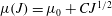
Another rheological property of our interest is the stress ratio,
 $\unicode[STIX]{x1D707}=\unicode[STIX]{x1D70E}_{xy}/P$
. It is known that
$\unicode[STIX]{x1D707}=\unicode[STIX]{x1D70E}_{xy}/P$
. It is known that
 $\unicode[STIX]{x1D707}$
converges to a constant in approaching the jamming point, while it varies on departure from the point, by experiments and simulations (GDR Midi 2004; Boyer et al.
Reference Boyer, Guazzelli and Pouliquen2011; Kuwano & Hatano Reference Kuwano and Hatano2011; Irani, Chaudhuri & Heussinger Reference Irani, Chaudhuri and Heussinger2014; Dagois-Bohy et al.
Reference Dagois-Bohy, Hormozi, Guazzelli and Pouliquen2015; Kawasaki et al.
Reference Kawasaki, Coslovich, Ikeda and Berthier2015). In fact, a constitutive equation for
$\unicode[STIX]{x1D707}$
converges to a constant in approaching the jamming point, while it varies on departure from the point, by experiments and simulations (GDR Midi 2004; Boyer et al.
Reference Boyer, Guazzelli and Pouliquen2011; Kuwano & Hatano Reference Kuwano and Hatano2011; Irani, Chaudhuri & Heussinger Reference Irani, Chaudhuri and Heussinger2014; Dagois-Bohy et al.
Reference Dagois-Bohy, Hormozi, Guazzelli and Pouliquen2015; Kawasaki et al.
Reference Kawasaki, Coslovich, Ikeda and Berthier2015). In fact, a constitutive equation for
 $\unicode[STIX]{x1D707}(J)=\unicode[STIX]{x1D70E}_{xy}/P$
together with
$\unicode[STIX]{x1D707}(J)=\unicode[STIX]{x1D70E}_{xy}/P$
together with
 $\unicode[STIX]{x1D711}=\unicode[STIX]{x1D711}(J)$
, where
$\unicode[STIX]{x1D711}=\unicode[STIX]{x1D711}(J)$
, where
 $J=\dot{\unicode[STIX]{x1D6FE}}\unicode[STIX]{x1D702}_{0}/P$
is the viscous number, is proposed and confirmed by experiments conducted with a pressure-imposed cell (
$J=\dot{\unicode[STIX]{x1D6FE}}\unicode[STIX]{x1D702}_{0}/P$
is the viscous number, is proposed and confirmed by experiments conducted with a pressure-imposed cell (
 $\unicode[STIX]{x1D707}$
–
$\unicode[STIX]{x1D707}$
–
 $J$
rheology) (Boyer et al.
Reference Boyer, Guazzelli and Pouliquen2011; Dagois-Bohy et al.
Reference Dagois-Bohy, Hormozi, Guazzelli and Pouliquen2015). The reported result exhibits
$J$
rheology) (Boyer et al.
Reference Boyer, Guazzelli and Pouliquen2011; Dagois-Bohy et al.
Reference Dagois-Bohy, Hormozi, Guazzelli and Pouliquen2015). The reported result exhibits
 $\unicode[STIX]{x1D707}(J)=\unicode[STIX]{x1D707}_{0}+CJ^{1/2}$
, where
$\unicode[STIX]{x1D707}(J)=\unicode[STIX]{x1D707}_{0}+CJ^{1/2}$
, where
 $C$
is a constant and
$C$
is a constant and
 $\unicode[STIX]{x1D707}_{0}$
is its value in the jamming limit,
$\unicode[STIX]{x1D707}_{0}$
is its value in the jamming limit,
 $J\rightarrow 0$
. However, there exists no theory to explain this law so far.
$J\rightarrow 0$
. However, there exists no theory to explain this law so far.
Derivation of the rheological properties of suspensions from a microscopic theory is difficult even for the shear viscosity. It has been shown by Brady and his coworkers that the effective self-diffusion constant satisfies
 $D(\unicode[STIX]{x1D711})\propto D_{0}(\unicode[STIX]{x1D711}_{m}-\unicode[STIX]{x1D711})$
, where
$D(\unicode[STIX]{x1D711})\propto D_{0}(\unicode[STIX]{x1D711}_{m}-\unicode[STIX]{x1D711})$
, where
 $D_{0}=T_{s}/(3\unicode[STIX]{x03C0}\,\text{d}\unicode[STIX]{x1D702}_{0})$
with
$D_{0}=T_{s}/(3\unicode[STIX]{x03C0}\,\text{d}\unicode[STIX]{x1D702}_{0})$
with
 $T_{s}$
the solvent temperature, which is crucial to obtain
$T_{s}$
the solvent temperature, which is crucial to obtain
 $\unicode[STIX]{x1D702}_{s}(\unicode[STIX]{x1D711})/\unicode[STIX]{x1D702}_{0}\sim (\unicode[STIX]{x1D711}_{m}-\unicode[STIX]{x1D711})^{-2}$
for Brownian suspensions (Brady Reference Brady1993; Brady & Morris Reference Brady and Morris1997; Foss & Brady Reference Foss and Brady2000). However, this theory is not applicable to non-Brownian suspensions, because
$\unicode[STIX]{x1D702}_{s}(\unicode[STIX]{x1D711})/\unicode[STIX]{x1D702}_{0}\sim (\unicode[STIX]{x1D711}_{m}-\unicode[STIX]{x1D711})^{-2}$
for Brownian suspensions (Brady Reference Brady1993; Brady & Morris Reference Brady and Morris1997; Foss & Brady Reference Foss and Brady2000). However, this theory is not applicable to non-Brownian suspensions, because
 $D(\unicode[STIX]{x1D711})$
is an increasing function of
$D(\unicode[STIX]{x1D711})$
is an increasing function of
 $\unicode[STIX]{x1D711}$
in non-Brownian suspensions (Leighton & Acrivos Reference Leighton and Acrivos1987a
,Reference Leighton and Acrivos
b
; Breedveld et al.
Reference Breedveld, van den Ende, Tripathi and Acrivos1998, Reference Breedveld, van den Ende, Bosscher, Jongschaap and Mellema2002; Heussinger, Berthier & Barrat Reference Heussinger, Berthier and Barrat2010; Olsson Reference Olsson2010). Hence, an alternative framework is necessary for dense non-Brownian suspensions. In this paper, we attempt to derive the divergent behaviour of the shear and pressure viscosities,
$\unicode[STIX]{x1D711}$
in non-Brownian suspensions (Leighton & Acrivos Reference Leighton and Acrivos1987a
,Reference Leighton and Acrivos
b
; Breedveld et al.
Reference Breedveld, van den Ende, Tripathi and Acrivos1998, Reference Breedveld, van den Ende, Bosscher, Jongschaap and Mellema2002; Heussinger, Berthier & Barrat Reference Heussinger, Berthier and Barrat2010; Olsson Reference Olsson2010). Hence, an alternative framework is necessary for dense non-Brownian suspensions. In this paper, we attempt to derive the divergent behaviour of the shear and pressure viscosities,
 $\unicode[STIX]{x1D702}_{s}/\unicode[STIX]{x1D702}_{0}\sim \unicode[STIX]{x1D702}_{n}/\unicode[STIX]{x1D702}_{0}\sim (\unicode[STIX]{x1D711}_{J}-\unicode[STIX]{x1D711})^{-2}$
, and the
$\unicode[STIX]{x1D702}_{s}/\unicode[STIX]{x1D702}_{0}\sim \unicode[STIX]{x1D702}_{n}/\unicode[STIX]{x1D702}_{0}\sim (\unicode[STIX]{x1D711}_{J}-\unicode[STIX]{x1D711})^{-2}$
, and the
 $\unicode[STIX]{x1D707}$
–
$\unicode[STIX]{x1D707}$
–
 $J$
rheology,
$J$
rheology,
 $\unicode[STIX]{x1D707}(J)=\unicode[STIX]{x1D707}_{0}+CJ^{1/2}$
, by means of a microscopic theory for an idealistic model of non-Brownian suspensions.
$\unicode[STIX]{x1D707}(J)=\unicode[STIX]{x1D707}_{0}+CJ^{1/2}$
, by means of a microscopic theory for an idealistic model of non-Brownian suspensions.
2 Basic equations and exact equations for the stress
2.1 Microscopic basic equations
We consider an assembly of
 $N$
frictionless monodisperse spherical particles of diameter
$N$
frictionless monodisperse spherical particles of diameter
 $d$
contained in a box of volume
$d$
contained in a box of volume
 $V$
and immersed in a liquid of viscosity
$V$
and immersed in a liquid of viscosity
 $\unicode[STIX]{x1D702}_{0}$
. A simple steady shear with shear rate
$\unicode[STIX]{x1D702}_{0}$
. A simple steady shear with shear rate
 $\dot{\unicode[STIX]{x1D6FE}}$
is applied to the system. The coordinate is chosen such that the flow is in the
$\dot{\unicode[STIX]{x1D6FE}}$
is applied to the system. The coordinate is chosen such that the flow is in the
 $x$
-direction and the velocity gradient is in the
$x$
-direction and the velocity gradient is in the
 $y$
-direction. We consider the overdamped equation of motion
$y$
-direction. We consider the overdamped equation of motion
 $$\begin{eqnarray}\displaystyle \mathop{\sum }_{j=1}^{N}\unicode[STIX]{x1D701}_{ij}^{(N)}(\dot{\boldsymbol{r}}_{j}-\dot{\unicode[STIX]{x1D6FE}}y_{j}\boldsymbol{e}_{x})=\boldsymbol{F}_{i}^{(p)}\quad (i=1,\ldots ,N), & & \displaystyle\end{eqnarray}$$
where
 $\boldsymbol{r}_{i}$
and
$\boldsymbol{r}_{i}$
and
 $\dot{\boldsymbol{r}}_{i}$
are the position and velocity of particle
$\dot{\boldsymbol{r}}_{i}$
are the position and velocity of particle
 $i$
, respectively,
$i$
, respectively,
 $\boldsymbol{e}_{x}$
is the unit vector in the
$\boldsymbol{e}_{x}$
is the unit vector in the
 $x$
-direction,
$x$
-direction,
 $\boldsymbol{F}_{i}^{(p)}$
is the interparticle force exerted on particle
$\boldsymbol{F}_{i}^{(p)}$
is the interparticle force exerted on particle
 $i$
from other particles and
$i$
from other particles and
 $\{\unicode[STIX]{x1D701}_{ij}^{(N)}\}\text{}_{i,j=1}^{N}$
is the resistance matrix of the suspension, which depends on the configuration of the particles,
$\{\unicode[STIX]{x1D701}_{ij}^{(N)}\}\text{}_{i,j=1}^{N}$
is the resistance matrix of the suspension, which depends on the configuration of the particles,
 $\{\boldsymbol{r}_{i}\}\text{}_{i=1}^{N}$
. Note that
$\{\boldsymbol{r}_{i}\}\text{}_{i=1}^{N}$
. Note that
 $\{\unicode[STIX]{x1D701}_{ij}^{(N)}\}\text{}_{i,j=1}^{N}$
is a
$\{\unicode[STIX]{x1D701}_{ij}^{(N)}\}\text{}_{i,j=1}^{N}$
is a
 $3N\times 3N$
matrix, where each component
$3N\times 3N$
matrix, where each component
 $\unicode[STIX]{x1D701}_{ij}^{(N)}$
is a
$\unicode[STIX]{x1D701}_{ij}^{(N)}$
is a
 $3\times 3$
matrix. In particle suspensions, the inertia of the particles is absorbed by the background fluid and hence insignificant. Thus we neglect it in (2.1). We also neglect the rotation of the particles and the thermal fluctuating force exerted on the particles from the solvent in (2.1).
$3\times 3$
matrix. In particle suspensions, the inertia of the particles is absorbed by the background fluid and hence insignificant. Thus we neglect it in (2.1). We also neglect the rotation of the particles and the thermal fluctuating force exerted on the particles from the solvent in (2.1).
The time evolution of an arbitrary observable
 $A(\unicode[STIX]{x1D71E})$
is determined by the Liouville equation
$A(\unicode[STIX]{x1D71E})$
is determined by the Liouville equation
 $$\begin{eqnarray}\displaystyle {\dot{A}}(\unicode[STIX]{x1D71E}(t))=\dot{\unicode[STIX]{x1D71E}}\boldsymbol{\cdot }\frac{\unicode[STIX]{x2202}}{\unicode[STIX]{x2202}\unicode[STIX]{x1D71E}}A(\unicode[STIX]{x1D71E}(t)):=\text{i}{\mathcal{L}}A(\unicode[STIX]{x1D71E}(t)), & & \displaystyle\end{eqnarray}$$
where
 $\text{i}{\mathcal{L}}$
is the Liouvillian. In simple shear flows,
$\text{i}{\mathcal{L}}$
is the Liouvillian. In simple shear flows,
 $\unicode[STIX]{x1D71E}$
is given by
$\unicode[STIX]{x1D71E}$
is given by
 $\unicode[STIX]{x1D71E}=\{\boldsymbol{r}_{i},\boldsymbol{v}_{i}\}\text{}_{i=1}^{N}$
, where
$\unicode[STIX]{x1D71E}=\{\boldsymbol{r}_{i},\boldsymbol{v}_{i}\}\text{}_{i=1}^{N}$
, where
 $$\begin{eqnarray}\displaystyle \boldsymbol{v}_{i}:=\dot{\boldsymbol{r}}_{i}-\dot{\unicode[STIX]{x1D6FE}}y_{i}\boldsymbol{e}_{x}=\mathop{\sum }_{j=1}^{N}\unicode[STIX]{x1D701}_{ij}^{(N)-1}\boldsymbol{F}_{j}^{(p)} & & \displaystyle\end{eqnarray}$$
is the peculiar velocity, which is the velocity in the sheared frame. For (2.1),
 $\text{i}{\mathcal{L}}$
is given by
$\text{i}{\mathcal{L}}$
is given by
 $$\begin{eqnarray}\displaystyle \text{i}{\mathcal{L}}:=\mathop{\sum }_{i=1}^{N}\left(\boldsymbol{v}_{i}\boldsymbol{\cdot }\frac{\unicode[STIX]{x2202}}{\unicode[STIX]{x2202}\boldsymbol{r}_{i}}+\dot{\boldsymbol{v}}_{i}\boldsymbol{\cdot }\frac{\unicode[STIX]{x2202}}{\unicode[STIX]{x2202}\boldsymbol{v}_{i}}\right)=\mathop{\sum }_{i=1}^{N}\left(\mathop{\sum }_{j=1}^{N}\unicode[STIX]{x1D701}_{ij}^{(N)-1}\boldsymbol{F}_{j}^{(p)}\boldsymbol{\cdot }\frac{\unicode[STIX]{x2202}}{\unicode[STIX]{x2202}\boldsymbol{r}_{i}}+\dot{\boldsymbol{v}}_{i}\boldsymbol{\cdot }\frac{\unicode[STIX]{x2202}}{\unicode[STIX]{x2202}\boldsymbol{v}_{i}}\right), & & \displaystyle\end{eqnarray}$$
where
 $\dot{\boldsymbol{v}}_{i}$
is evaluated as
$\dot{\boldsymbol{v}}_{i}$
is evaluated as
 $$\begin{eqnarray}\displaystyle \dot{\boldsymbol{v}}_{i}=\ddot{\boldsymbol{r}}_{i}-\dot{\unicode[STIX]{x1D6FE}}{\dot{y}}_{i}\boldsymbol{e}_{x}=\ddot{\boldsymbol{r}}_{i}-\dot{\unicode[STIX]{x1D6FE}}\mathop{\sum }_{j=1}^{N}\unicode[STIX]{x1D701}_{ij}^{(N)-1}F_{j,y}^{(p)}\boldsymbol{e}_{x}. & & \displaystyle\end{eqnarray}$$
Note that (2.3) is utilized in the second equality of (2.5). In the formulation of overdamped Liouville equation, we neglect
 $\ddot{\boldsymbol{r}}_{i}$
in (2.5), because
$\ddot{\boldsymbol{r}}_{i}$
in (2.5), because
 $\boldsymbol{v}_{i}$
rather than
$\boldsymbol{v}_{i}$
rather than
 $\ddot{\boldsymbol{r}}_{i}$
resides in the equation of motion, equation (2.3). This leads us to the expression
$\ddot{\boldsymbol{r}}_{i}$
resides in the equation of motion, equation (2.3). This leads us to the expression
 $$\begin{eqnarray}\displaystyle \text{i}{\mathcal{L}}=\mathop{\sum }_{i=1}^{N}\left(\mathop{\sum }_{j=1}^{N}\unicode[STIX]{x1D701}_{ij}^{(N)-1}\boldsymbol{F}_{j}^{(p)}\boldsymbol{\cdot }\frac{\unicode[STIX]{x2202}}{\unicode[STIX]{x2202}\boldsymbol{r}_{i}}-\dot{\unicode[STIX]{x1D6FE}}F_{i,y}^{(p)}\frac{\unicode[STIX]{x2202}}{\unicode[STIX]{x2202}F_{i,x}^{(p)}}\right). & & \displaystyle\end{eqnarray}$$
Note, however, that neglecting
 $\ddot{\boldsymbol{r}}_{i}$
in (2.5) does not mean the absence of
$\ddot{\boldsymbol{r}}_{i}$
in (2.5) does not mean the absence of
 $\dot{\boldsymbol{v}}_{i}$
as can be seen in (2.5). In fact, because of the existence of
$\dot{\boldsymbol{v}}_{i}$
as can be seen in (2.5). In fact, because of the existence of
 $\boldsymbol{v}_{i}$
, trajectories of the particles can be curved.
$\boldsymbol{v}_{i}$
, trajectories of the particles can be curved.
The Liouville equation of the microscopic stress tensor
 $\tilde{\unicode[STIX]{x1D70E}}_{\unicode[STIX]{x1D6FC}\unicode[STIX]{x1D6FD}}(\unicode[STIX]{x1D71E})$
(
$\tilde{\unicode[STIX]{x1D70E}}_{\unicode[STIX]{x1D6FC}\unicode[STIX]{x1D6FD}}(\unicode[STIX]{x1D71E})$
(
 $\unicode[STIX]{x1D6FC},\unicode[STIX]{x1D6FD}=x,y,z$
) reads
$\unicode[STIX]{x1D6FC},\unicode[STIX]{x1D6FD}=x,y,z$
) reads
 $$\begin{eqnarray}\displaystyle \frac{\text{d}}{\text{d}t}\tilde{\unicode[STIX]{x1D70E}}_{\unicode[STIX]{x1D6FC}\unicode[STIX]{x1D6FD}}(\unicode[STIX]{x1D71E})=\mathop{\sum }_{i=1}^{N}\left(\mathop{\sum }_{j=1}^{N}\unicode[STIX]{x1D701}_{ij}^{(N)-1}\boldsymbol{F}_{j}^{(p)}\boldsymbol{\cdot }\frac{\unicode[STIX]{x2202}\tilde{\unicode[STIX]{x1D70E}}_{\unicode[STIX]{x1D6FC}\unicode[STIX]{x1D6FD}}(\unicode[STIX]{x1D71E})}{\unicode[STIX]{x2202}\boldsymbol{r}_{i}}-\dot{\unicode[STIX]{x1D6FE}}F_{i,y}^{(p)}\frac{\unicode[STIX]{x2202}\tilde{\unicode[STIX]{x1D70E}}_{\unicode[STIX]{x1D6FC}\unicode[STIX]{x1D6FD}}(\unicode[STIX]{x1D71E})}{\unicode[STIX]{x2202}F_{i,x}^{(p)}}\right), & & \displaystyle\end{eqnarray}$$
where
 $\tilde{\unicode[STIX]{x1D70E}}_{\unicode[STIX]{x1D6FC}\unicode[STIX]{x1D6FD}}(\unicode[STIX]{x1D71E})$
is given by
$\tilde{\unicode[STIX]{x1D70E}}_{\unicode[STIX]{x1D6FC}\unicode[STIX]{x1D6FD}}(\unicode[STIX]{x1D71E})$
is given by
 $$\begin{eqnarray}\displaystyle \tilde{\unicode[STIX]{x1D70E}}_{\unicode[STIX]{x1D6FC}\unicode[STIX]{x1D6FD}}(\unicode[STIX]{x1D71E}):=-\frac{1}{2V}\mathop{\sum }_{i=1}^{N}(r_{i,\unicode[STIX]{x1D6FD}}F_{i,\unicode[STIX]{x1D6FC}}^{(p)}+r_{i,\unicode[STIX]{x1D6FC}}F_{i,\unicode[STIX]{x1D6FD}}^{(p)}). & & \displaystyle\end{eqnarray}$$
In simple shear flows, the only non-zero components of
 $\tilde{\unicode[STIX]{x1D70E}}_{\unicode[STIX]{x1D6FC}\unicode[STIX]{x1D6FD}}(\unicode[STIX]{x1D71E})$
are
$\tilde{\unicode[STIX]{x1D70E}}_{\unicode[STIX]{x1D6FC}\unicode[STIX]{x1D6FD}}(\unicode[STIX]{x1D71E})$
are
 $\tilde{\unicode[STIX]{x1D70E}}_{xy}(\unicode[STIX]{x1D71E})$
and the diagonal ones, from which the microscopic pressure is given by
$\tilde{\unicode[STIX]{x1D70E}}_{xy}(\unicode[STIX]{x1D71E})$
and the diagonal ones, from which the microscopic pressure is given by
 $\tilde{P}(\unicode[STIX]{x1D71E})=-(\tilde{\unicode[STIX]{x1D70E}}_{xx}(\unicode[STIX]{x1D71E})+\tilde{\unicode[STIX]{x1D70E}}_{yy}(\unicode[STIX]{x1D71E})+\tilde{\unicode[STIX]{x1D70E}}_{zz}(\unicode[STIX]{x1D71E}))/3$
. Note that we mainly consider the Cauchy stress, which contributes to the divergence at
$\tilde{P}(\unicode[STIX]{x1D71E})=-(\tilde{\unicode[STIX]{x1D70E}}_{xx}(\unicode[STIX]{x1D71E})+\tilde{\unicode[STIX]{x1D70E}}_{yy}(\unicode[STIX]{x1D71E})+\tilde{\unicode[STIX]{x1D70E}}_{zz}(\unicode[STIX]{x1D71E}))/3$
. Note that we mainly consider the Cauchy stress, which contributes to the divergence at
 $\unicode[STIX]{x1D711}\approx \unicode[STIX]{x1D711}_{J}$
, but it is possible to define the kinetic stress by the peculiar velocity.
$\unicode[STIX]{x1D711}\approx \unicode[STIX]{x1D711}_{J}$
, but it is possible to define the kinetic stress by the peculiar velocity.
2.2 Exact equations for the stress
Macroscopic equation of continuity of the stress tensor is obtained by multiplying (2.7) by the non-equilibrium distribution function
 $f(\unicode[STIX]{x1D71E},t)$
and integrating over
$f(\unicode[STIX]{x1D71E},t)$
and integrating over
 $\unicode[STIX]{x1D71E}$
,
$\unicode[STIX]{x1D71E}$
,
 $$\begin{eqnarray}\displaystyle & & \displaystyle \frac{\text{d}}{\text{d}t}\unicode[STIX]{x1D70E}_{\unicode[STIX]{x1D6FC}\unicode[STIX]{x1D6FD}}+\frac{1}{2}\dot{\unicode[STIX]{x1D6FE}}(\unicode[STIX]{x1D6FF}_{\unicode[STIX]{x1D6FC}x}\unicode[STIX]{x1D70E}_{y\unicode[STIX]{x1D6FD}}+\unicode[STIX]{x1D6FF}_{\unicode[STIX]{x1D6FD}x}\unicode[STIX]{x1D70E}_{y\unicode[STIX]{x1D6FC}})=-\frac{1}{2V}\mathop{\sum }_{i}\left\langle \mathop{\sum }_{j}\unicode[STIX]{x1D701}_{ij}^{(N)-1}F_{j,\unicode[STIX]{x1D6FD}}^{(p)}F_{i,\unicode[STIX]{x1D6FC}}^{(p)}\right\rangle +(\unicode[STIX]{x1D6FC}\leftrightarrow \unicode[STIX]{x1D6FD})\nonumber\\ \displaystyle & & \displaystyle \quad -\,\frac{1}{2V}\sum _{i,j}\left\langle \mathop{\sum }_{k}\unicode[STIX]{x1D701}_{ik}^{(N)-1}F_{k,\unicode[STIX]{x1D706}}^{(p)}r_{j,\unicode[STIX]{x1D6FD}}\frac{\unicode[STIX]{x2202}F_{j,\unicode[STIX]{x1D6FC}}^{(p)}}{\unicode[STIX]{x2202}r_{i,\unicode[STIX]{x1D706}}}\right\rangle +(\unicode[STIX]{x1D6FC}\leftrightarrow \unicode[STIX]{x1D6FD}),\end{eqnarray}$$
where
 $$\begin{eqnarray}\displaystyle \langle \cdots \rangle :=\int \text{d}\unicode[STIX]{x1D71E}f(\unicode[STIX]{x1D71E},t)\cdots & & \displaystyle\end{eqnarray}$$
is the macroscopic average,
 $\sum _{i,j}^{\prime }$
denotes the summation over
$\sum _{i,j}^{\prime }$
denotes the summation over
 $i$
and
$i$
and
 $j$
with
$j$
with
 $i\neq j$
and the macroscopic stress tensor denotes
$i\neq j$
and the macroscopic stress tensor denotes
 $$\begin{eqnarray}\displaystyle \unicode[STIX]{x1D70E}_{\unicode[STIX]{x1D6FC}\unicode[STIX]{x1D6FD}}:=\int \text{d}\unicode[STIX]{x1D71E}f(\unicode[STIX]{x1D71E},t)\tilde{\unicode[STIX]{x1D70E}}_{\unicode[STIX]{x1D6FC}\unicode[STIX]{x1D6FD}}(\unicode[STIX]{x1D71E}). & & \displaystyle\end{eqnarray}$$
It might be noteworthy that the equation of continuity of the stress tensor, equation (2.9), is consistent with that for the Enskog theory of moderately dense inertial suspensions (Hayakawa, Takada & Garzó Reference Hayakawa, Takada and Garzó2017). In fact, the two terms on the right-hand side of (2.9), which are proportional to
 $\unicode[STIX]{x1D701}_{ij}^{(N)-1}$
and originate from particle contacts, correspond to the collision integral terms in the Enskog theory.
$\unicode[STIX]{x1D701}_{ij}^{(N)-1}$
and originate from particle contacts, correspond to the collision integral terms in the Enskog theory.
3 Approximate expression of the interparticle force for dense frictionless hard spheres
To proceed, let us derive the specific form of the interparticle force
 $\boldsymbol{F}_{i}^{(p)}(\{\boldsymbol{r}_{j}\}\text{}_{j=1}^{N})$
for dense frictionless hard spheres. For dense spheres where all of them are at or close to contact, we can expect that the far-field part of
$\boldsymbol{F}_{i}^{(p)}(\{\boldsymbol{r}_{j}\}\text{}_{j=1}^{N})$
for dense frictionless hard spheres. For dense spheres where all of them are at or close to contact, we can expect that the far-field part of
 $\overleftrightarrow{\unicode[STIX]{x1D701}^{(N)}}(\{\boldsymbol{r}_{i}\}\text{}_{i=1}^{N})$
does not contribute and only the lubrication part, which is well approximated by the sum of the two-body terms
$\overleftrightarrow{\unicode[STIX]{x1D701}^{(N)}}(\{\boldsymbol{r}_{i}\}\text{}_{i=1}^{N})$
does not contribute and only the lubrication part, which is well approximated by the sum of the two-body terms
 $\overleftrightarrow{\unicode[STIX]{x1D701}_{lub}^{(2)}}(\boldsymbol{r}_{ij})$
, is significant (Kim & Karrila Reference Kim and Karrila2005; Seto et al.
Reference Seto, Mari, Morris and Denn2013; Mari et al.
Reference Mari, Seto, Morris and Denn2014). Thus, we approximate the resistance matrix
$\overleftrightarrow{\unicode[STIX]{x1D701}_{lub}^{(2)}}(\boldsymbol{r}_{ij})$
, is significant (Kim & Karrila Reference Kim and Karrila2005; Seto et al.
Reference Seto, Mari, Morris and Denn2013; Mari et al.
Reference Mari, Seto, Morris and Denn2014). Thus, we approximate the resistance matrix
 $\overleftrightarrow{\unicode[STIX]{x1D701}^{(N)}}$
as
$\overleftrightarrow{\unicode[STIX]{x1D701}^{(N)}}$
as
 $$\begin{eqnarray}\displaystyle \overleftrightarrow{\unicode[STIX]{x1D701}^{(N)}}(\{\boldsymbol{r}_{i}\}\text{}_{i=1}^{N})\approx \unicode[STIX]{x1D701}_{0}\unicode[STIX]{x1D644}+\overleftrightarrow{\unicode[STIX]{x1D701}_{lub}^{(2)}}(\boldsymbol{r}_{ij}), & & \displaystyle\end{eqnarray}$$
where the first term on the right-hand side with
 $\unicode[STIX]{x1D701}_{0}:=3\unicode[STIX]{x03C0}\unicode[STIX]{x1D702}_{0}d$
and
$\unicode[STIX]{x1D701}_{0}:=3\unicode[STIX]{x03C0}\unicode[STIX]{x1D702}_{0}d$
and
 $\unicode[STIX]{x1D644}$
the unit matrix is the Stokesean one-body drag force. This leads to the approximate equation of motion
$\unicode[STIX]{x1D644}$
the unit matrix is the Stokesean one-body drag force. This leads to the approximate equation of motion
 $$\begin{eqnarray}\displaystyle \unicode[STIX]{x1D701}_{0}(\dot{\boldsymbol{r}}_{i}-\dot{\unicode[STIX]{x1D6FE}}y_{i}\boldsymbol{e}_{x})+\mathop{\sum }_{j\neq i}\unicode[STIX]{x1D701}_{lub,ij}^{(2)}(\dot{\boldsymbol{r}}_{j}-\dot{\unicode[STIX]{x1D6FE}}y_{j}\boldsymbol{e}_{x})\approx \boldsymbol{F}_{i}^{(p)}. & & \displaystyle\end{eqnarray}$$
Then, accordingly, the interparticle force should be well approximated by a sum of two-body forces,
 $$\begin{eqnarray}\displaystyle \boldsymbol{F}_{i}^{(p)}\approx \mathop{\sum }_{j\neq i}\boldsymbol{F}_{ij}^{(p)}, & & \displaystyle\end{eqnarray}$$
where
 $\boldsymbol{F}_{ij}^{(p)}$
is the two-body force exerted on particle
$\boldsymbol{F}_{ij}^{(p)}$
is the two-body force exerted on particle
 $i$
from
$i$
from
 $j$
. The dynamics of the interacting two spheres is schematically described in figure 2. When the approaching two spheres come into contact (a), they slide in the tangential direction until they are aligned in the velocity-gradient direction (b), and then depart (c). In general, there are not only two but multiple of particles in contact, but every pair slides mutually in the tangential direction until their departure, so it is reasonable to consider the dynamics as a superposition of the two-body counterpart. Indeed, the simulation in terms of Stokesean dynamics is performed in terms of the superposition of the two-body interactions (Seto et al.
Reference Seto, Mari, Morris and Denn2013; Mari et al.
Reference Mari, Seto, Morris and Denn2014). Hence, it is sufficient to consider the two-body dynamics to determine
$j$
. The dynamics of the interacting two spheres is schematically described in figure 2. When the approaching two spheres come into contact (a), they slide in the tangential direction until they are aligned in the velocity-gradient direction (b), and then depart (c). In general, there are not only two but multiple of particles in contact, but every pair slides mutually in the tangential direction until their departure, so it is reasonable to consider the dynamics as a superposition of the two-body counterpart. Indeed, the simulation in terms of Stokesean dynamics is performed in terms of the superposition of the two-body interactions (Seto et al.
Reference Seto, Mari, Morris and Denn2013; Mari et al.
Reference Mari, Seto, Morris and Denn2014). Hence, it is sufficient to consider the two-body dynamics to determine
 $\boldsymbol{F}_{ij}^{(p)}$
.
$\boldsymbol{F}_{ij}^{(p)}$
.
Let us consider two spheres
 $i$
and
$i$
and
 $j$
in contact. The equation of motion of the two spheres is given by
$j$
in contact. The equation of motion of the two spheres is given by
 $$\begin{eqnarray}\displaystyle \unicode[STIX]{x1D701}_{0}\left[\begin{array}{@{}c@{}}\dot{\boldsymbol{r}}_{i}-\dot{\unicode[STIX]{x1D6FE}}y_{i}\boldsymbol{e}_{x}\\ \dot{\boldsymbol{r}}_{j}-\dot{\unicode[STIX]{x1D6FE}}y_{j}\boldsymbol{e}_{x}\end{array}\right]+\overleftrightarrow{\unicode[STIX]{x1D701}_{lub}^{(2)}}(\boldsymbol{r}_{ij})\left[\begin{array}{@{}c@{}}\dot{\boldsymbol{r}}_{i}-\dot{\unicode[STIX]{x1D6FE}}y_{i}\boldsymbol{e}_{x}\\ \dot{\boldsymbol{r}}_{j}-\dot{\unicode[STIX]{x1D6FE}}y_{j}\boldsymbol{e}_{x}\end{array}\right]=\left[\begin{array}{@{}c@{}}\boldsymbol{F}_{ij}^{(p)}\\ -\boldsymbol{F}_{ij}^{(p)}\end{array}\right], & & \displaystyle\end{eqnarray}$$
where we have utilized
 $\boldsymbol{F}_{ji}^{(p)}=-\boldsymbol{F}_{ij}^{(p)}$
. The matrix
$\boldsymbol{F}_{ji}^{(p)}=-\boldsymbol{F}_{ij}^{(p)}$
. The matrix
 $\overleftrightarrow{\unicode[STIX]{x1D701}_{lub}^{(2)}}$
is explicitly given by (Jeffrey & Onishi Reference Jeffrey and Onishi1984)
$\overleftrightarrow{\unicode[STIX]{x1D701}_{lub}^{(2)}}$
is explicitly given by (Jeffrey & Onishi Reference Jeffrey and Onishi1984)
 $$\begin{eqnarray}\displaystyle & \displaystyle \overleftrightarrow{\unicode[STIX]{x1D701}_{lub}^{(2)}}(\boldsymbol{r}_{ij})=\unicode[STIX]{x1D701}_{0}\left[\begin{array}{@{}cc@{}}\unicode[STIX]{x1D6F1}(\boldsymbol{r}_{ij}) & -\unicode[STIX]{x1D6F1}(\boldsymbol{r}_{ij})\\ -\unicode[STIX]{x1D6F1}(\boldsymbol{r}_{ij}) & \unicode[STIX]{x1D6F1}(\boldsymbol{r}_{ij})\end{array}\right], & \displaystyle\end{eqnarray}$$
 $$\begin{eqnarray}\displaystyle & \displaystyle \unicode[STIX]{x1D6F1}(\boldsymbol{r}_{ij}):=\frac{1}{8}\frac{1}{\unicode[STIX]{x1D6FF}r_{ij}+\unicode[STIX]{x1D716}}P_{ij}+\frac{1}{12}\ln \frac{1}{\unicode[STIX]{x1D6FF}r_{ij}+\unicode[STIX]{x1D716}}P_{ij}^{\prime }, & \displaystyle\end{eqnarray}$$
where
 $\unicode[STIX]{x1D701}_{0}:=3\unicode[STIX]{x03C0}\unicode[STIX]{x1D702}_{0}d$
,
$\unicode[STIX]{x1D701}_{0}:=3\unicode[STIX]{x03C0}\unicode[STIX]{x1D702}_{0}d$
,
 $\unicode[STIX]{x1D6FF}r_{ij}:=r_{ij}-d$
and
$\unicode[STIX]{x1D6FF}r_{ij}:=r_{ij}-d$
and
 $P_{ij}:=\hat{\boldsymbol{r}}_{ij}\hat{\boldsymbol{r}}_{ij}$
,
$P_{ij}:=\hat{\boldsymbol{r}}_{ij}\hat{\boldsymbol{r}}_{ij}$
,
 $P_{ij}^{\prime }:=\unicode[STIX]{x1D644}-\hat{\boldsymbol{r}}_{ij}\hat{\boldsymbol{r}}_{ij}$
are projection operators. At contact, i.e.
$P_{ij}^{\prime }:=\unicode[STIX]{x1D644}-\hat{\boldsymbol{r}}_{ij}\hat{\boldsymbol{r}}_{ij}$
are projection operators. At contact, i.e.
 $\unicode[STIX]{x1D6FF}r_{ij}=0$
,
$\unicode[STIX]{x1D6FF}r_{ij}=0$
,
 $\overleftrightarrow{\unicode[STIX]{x1D701}_{lub}^{(2)}}$
exhibits singularities of the form
$\overleftrightarrow{\unicode[STIX]{x1D701}_{lub}^{(2)}}$
exhibits singularities of the form
 $\unicode[STIX]{x1D716}^{-1}$
and
$\unicode[STIX]{x1D716}^{-1}$
and
 $\ln \unicode[STIX]{x1D716}^{-1}$
, where
$\ln \unicode[STIX]{x1D716}^{-1}$
, where
 $\unicode[STIX]{x1D716}$
is a cut off which is physically interpreted as e.g. surface roughness. In this work we keep
$\unicode[STIX]{x1D716}$
is a cut off which is physically interpreted as e.g. surface roughness. In this work we keep
 $\unicode[STIX]{x1D716}$
finite and do not consider these singularities. Then, equation (3.4) is given by
$\unicode[STIX]{x1D716}$
finite and do not consider these singularities. Then, equation (3.4) is given by
 $$\begin{eqnarray}\displaystyle & & \displaystyle \unicode[STIX]{x1D701}_{0}\left[\begin{array}{@{}c@{}}\displaystyle (\dot{\boldsymbol{r}}_{i}-\dot{\unicode[STIX]{x1D6FE}}y_{i}\boldsymbol{e}_{x})+\frac{1}{8\unicode[STIX]{x1D716}}P_{ij}\boldsymbol{\cdot }(\dot{\boldsymbol{r}}_{ij}-\dot{\unicode[STIX]{x1D6FE}}y_{ij}\boldsymbol{e}_{x})+\frac{1}{12}\ln \unicode[STIX]{x1D716}^{-1}P_{ij}^{\prime }\boldsymbol{\cdot }(\dot{\boldsymbol{r}}_{ij}-\dot{\unicode[STIX]{x1D6FE}}y_{ij}\boldsymbol{e}_{x})\\ \displaystyle (\dot{\boldsymbol{r}}_{j}-\dot{\unicode[STIX]{x1D6FE}}y_{j}\boldsymbol{e}_{x})-\frac{1}{8\unicode[STIX]{x1D716}}P_{ij}\boldsymbol{\cdot }(\dot{\boldsymbol{r}}_{ij}-\dot{\unicode[STIX]{x1D6FE}}y_{ij}\boldsymbol{e}_{x})-\frac{1}{12}\ln \unicode[STIX]{x1D716}^{-1}P_{ij}^{\prime }\boldsymbol{\cdot }(\dot{\boldsymbol{r}}_{ij}-\dot{\unicode[STIX]{x1D6FE}}y_{ij}\boldsymbol{e}_{x})\end{array}\right]\nonumber\\ \displaystyle & & \displaystyle \quad =\left[\begin{array}{@{}c@{}}\boldsymbol{F}_{ij}^{(p)}\\ -\boldsymbol{F}_{ij}^{(p)}\end{array}\right].\end{eqnarray}$$
By subtracting the two equations, equation (3.7) reduces to
 $$\begin{eqnarray}\displaystyle \boldsymbol{F}_{ij}^{(p)}=\unicode[STIX]{x1D701}_{0}\left[\frac{1}{2}(\dot{\boldsymbol{r}}_{ij}-\dot{\unicode[STIX]{x1D6FE}}y_{ij}\boldsymbol{e}_{x})+\frac{1}{8\unicode[STIX]{x1D716}}P_{ij}\boldsymbol{\cdot }(\dot{\boldsymbol{r}}_{ij}-\dot{\unicode[STIX]{x1D6FE}}y_{ij}\boldsymbol{e}_{x})+\frac{1}{12}\ln \unicode[STIX]{x1D716}^{-1}P_{ij}^{\prime }\boldsymbol{\cdot }(\dot{\boldsymbol{r}}_{ij}-\dot{\unicode[STIX]{x1D6FE}}y_{ij}\boldsymbol{e}_{x})\right], & & \displaystyle\end{eqnarray}$$
where the right-hand side consists of the Stokesean drag force (first term), the normal lubrication force (second term) and the tangential lubrication force (third term). These three terms are of the order of 1,
 $\unicode[STIX]{x1D716}^{-1}$
and
$\unicode[STIX]{x1D716}^{-1}$
and
 $\ln \unicode[STIX]{x1D716}^{-1}$
, respectively. The second term is dominant for
$\ln \unicode[STIX]{x1D716}^{-1}$
, respectively. The second term is dominant for
 $\unicode[STIX]{x1D716}\ll 1$
, so (3.8) is reduced to
$\unicode[STIX]{x1D716}\ll 1$
, so (3.8) is reduced to
 $$\begin{eqnarray}\displaystyle \boldsymbol{F}_{ij}^{(p)}\approx \frac{\unicode[STIX]{x1D701}_{0}}{8\unicode[STIX]{x1D716}}P_{ij}\boldsymbol{\cdot }(\dot{\boldsymbol{r}}_{ij}-\dot{\unicode[STIX]{x1D6FE}}y_{ij}\boldsymbol{e}_{x})=\frac{\unicode[STIX]{x1D701}_{0}}{8\unicode[STIX]{x1D716}}(\hat{\boldsymbol{r}}_{ij}\boldsymbol{\cdot }\dot{\boldsymbol{r}}_{ij}-\dot{\unicode[STIX]{x1D6FE}}r_{ij}{\hat{y}}_{ij}\hat{x}_{ij})\hat{\boldsymbol{r}}_{ij}. & & \displaystyle\end{eqnarray}$$
For hard spheres, the relative velocity of
 $i$
and
$i$
and
 $j$
is in the direction perpendicular to
$j$
is in the direction perpendicular to
 $\hat{\boldsymbol{r}}_{ij}$
in order not to overlap, i.e.
$\hat{\boldsymbol{r}}_{ij}$
in order not to overlap, i.e.
 $\hat{\boldsymbol{r}}_{ij}\boldsymbol{\cdot }\dot{\boldsymbol{r}}_{ij}=0$
or
$\hat{\boldsymbol{r}}_{ij}\boldsymbol{\cdot }\dot{\boldsymbol{r}}_{ij}=0$
or
 $P_{ij}\boldsymbol{\cdot }\dot{\boldsymbol{r}}_{ij}=0$
(cf. figure 2
a). Then we obtain
$P_{ij}\boldsymbol{\cdot }\dot{\boldsymbol{r}}_{ij}=0$
(cf. figure 2
a). Then we obtain
 $$\begin{eqnarray}\displaystyle \boldsymbol{F}_{ij}^{(p)}=-{\textstyle \frac{1}{2}}\unicode[STIX]{x1D701}_{e}\dot{\unicode[STIX]{x1D6FE}}r_{ij}\hat{x}_{ij}{\hat{y}}_{ij}\hat{\boldsymbol{r}}_{ij}, & & \displaystyle\end{eqnarray}$$
where we have defined
 $$\begin{eqnarray}\displaystyle \unicode[STIX]{x1D701}_{e}:=\frac{\unicode[STIX]{x1D701}_{0}}{4\unicode[STIX]{x1D716}}=\frac{3\unicode[STIX]{x03C0}\unicode[STIX]{x1D702}_{0}d}{4\unicode[STIX]{x1D716}}. & & \displaystyle\end{eqnarray}$$
Note that (3.10) is valid only at contact, i.e.
 $r_{ij}=d$
, and
$r_{ij}=d$
, and
 $\boldsymbol{F}_{ij}^{(p)}=0$
for
$\boldsymbol{F}_{ij}^{(p)}=0$
for
 $r_{ij}>d$
for hard spheres. That is,
$r_{ij}>d$
for hard spheres. That is,
 $\boldsymbol{F}_{ij}^{(p)}\propto \unicode[STIX]{x1D6FF}(r_{ij}-d)$
. Thus we modify (3.10) by replacing
$\boldsymbol{F}_{ij}^{(p)}\propto \unicode[STIX]{x1D6FF}(r_{ij}-d)$
. Thus we modify (3.10) by replacing
 $r_{ij}$
with
$r_{ij}$
with
 $d^{2}\unicode[STIX]{x1D6FF}(r_{ij}-d)$
,
$d^{2}\unicode[STIX]{x1D6FF}(r_{ij}-d)$
,
 $$\begin{eqnarray}\displaystyle \boldsymbol{F}_{ij}^{(p)}=-{\textstyle \frac{1}{2}}\unicode[STIX]{x1D701}_{e}\dot{\unicode[STIX]{x1D6FE}}d^{2}\unicode[STIX]{x1D6FF}(r_{ij}-d)\hat{x}_{ij}{\hat{y}}_{ij}\hat{\boldsymbol{r}}_{ij}. & & \displaystyle\end{eqnarray}$$
Note that
 $\boldsymbol{F}_{ij}^{(p)}\propto \unicode[STIX]{x1D6FF}(r_{ij}-d)$
results in an important feature that the spatial correlations are expressed solely by (Donev et al.
Reference Donev, Torquato and Stillinger2005)
$\boldsymbol{F}_{ij}^{(p)}\propto \unicode[STIX]{x1D6FF}(r_{ij}-d)$
results in an important feature that the spatial correlations are expressed solely by (Donev et al.
Reference Donev, Torquato and Stillinger2005)
 $$\begin{eqnarray}\displaystyle g_{0}(\unicode[STIX]{x1D711})\sim (\unicode[STIX]{x1D711}_{J}-\unicode[STIX]{x1D711})^{-1}, & & \displaystyle\end{eqnarray}$$
where there is no dependence on its spatial derivative,
 $g^{\prime }(r)$
, because our dynamics inhibits the overlap of the contacting particles.
$g^{\prime }(r)$
, because our dynamics inhibits the overlap of the contacting particles.
Furthermore, in order for
 $\boldsymbol{F}_{ij}^{(p)}$
to be a repulsive force,
$\boldsymbol{F}_{ij}^{(p)}$
to be a repulsive force,
 $\hat{x}_{ij}{\hat{y}}_{ij}<0$
is necessary. Hence, we introduce a projection operator
$\hat{x}_{ij}{\hat{y}}_{ij}<0$
is necessary. Hence, we introduce a projection operator
 $$\begin{eqnarray}\displaystyle {\mathcal{P}}(\hat{x},{\hat{y}}):=-\hat{x}{\hat{y}}\unicode[STIX]{x1D6E9}(-\hat{x}{\hat{y}})>0 & & \displaystyle\end{eqnarray}$$
to assure this property,
 $$\begin{eqnarray}\displaystyle \boldsymbol{F}_{ij}^{(p)}={\textstyle \frac{1}{2}}\unicode[STIX]{x1D701}_{e}\dot{\unicode[STIX]{x1D6FE}}d^{2}\unicode[STIX]{x1D6FF}(r_{ij}-d){\mathcal{P}}(\hat{x}_{ij},{\hat{y}}_{ij})\hat{\boldsymbol{r}}_{ij}. & & \displaystyle\end{eqnarray}$$
Here,
 $\unicode[STIX]{x1D6E9}(x)$
is Heaviside’s step function, i.e.
$\unicode[STIX]{x1D6E9}(x)$
is Heaviside’s step function, i.e.
 $\unicode[STIX]{x1D6E9}(x)=1$
for
$\unicode[STIX]{x1D6E9}(x)=1$
for
 $x>0$
and
$x>0$
and
 $\unicode[STIX]{x1D6E9}(x)=0$
otherwise. The projection operator in (3.15) implies that
$\unicode[STIX]{x1D6E9}(x)=0$
otherwise. The projection operator in (3.15) implies that
 $\boldsymbol{F}_{ij}^{(p)}$
is non-zero only when the separation vector of the contacting two spheres
$\boldsymbol{F}_{ij}^{(p)}$
is non-zero only when the separation vector of the contacting two spheres
 $\boldsymbol{r}_{ij}:=\boldsymbol{r}_{i}-\boldsymbol{r}_{j}$
is in the compression quadrant (cf. figure 1). This results from the approximation where we have neglected the first and third terms in the right-hand side of (3.8). In fact, these two terms are in general non-zero, irrespective of the direction of
$\boldsymbol{r}_{ij}:=\boldsymbol{r}_{i}-\boldsymbol{r}_{j}$
is in the compression quadrant (cf. figure 1). This results from the approximation where we have neglected the first and third terms in the right-hand side of (3.8). In fact, these two terms are in general non-zero, irrespective of the direction of
 $\boldsymbol{r}_{ij}$
. Hence, although the direction of
$\boldsymbol{r}_{ij}$
. Hence, although the direction of
 $\boldsymbol{r}_{ij}$
can be in any direction in dense suspensions, the dominant contribution of the interparticle force comes from configurations where
$\boldsymbol{r}_{ij}$
can be in any direction in dense suspensions, the dominant contribution of the interparticle force comes from configurations where
 $\boldsymbol{r}_{ij}$
is in the compression quadrant. To summarize, the equation of motion for dense hard-sphere suspensions is reduced to
$\boldsymbol{r}_{ij}$
is in the compression quadrant. To summarize, the equation of motion for dense hard-sphere suspensions is reduced to
 $$\begin{eqnarray}\displaystyle \unicode[STIX]{x1D701}_{0}(\dot{\boldsymbol{r}}_{i}-\dot{\unicode[STIX]{x1D6FE}}y_{i}\boldsymbol{e}_{x})+\mathop{\sum }_{j\neq i}\unicode[STIX]{x1D701}_{lub,ij}^{(2)}(\dot{\boldsymbol{r}}_{j}-\dot{\unicode[STIX]{x1D6FE}}y_{j}\boldsymbol{e}_{x})=\mathop{\sum }_{j\neq i}\boldsymbol{F}_{ij}^{(p)}, & & \displaystyle\end{eqnarray}$$
where the two-body interparticle force
 $\boldsymbol{F}_{ij}^{(p)}$
is given by (3.15), and the summation is over the contacting particles. Note that (3.16) is exact, under the assumption that the interparticle force is expressed as a superposition of two-body forces, equation (3.3), and hydrodynamic forces other than the lubrication force are neglected, equation (3.1).
$\boldsymbol{F}_{ij}^{(p)}$
is given by (3.15), and the summation is over the contacting particles. Note that (3.16) is exact, under the assumption that the interparticle force is expressed as a superposition of two-body forces, equation (3.3), and hydrodynamic forces other than the lubrication force are neglected, equation (3.1).

Figure 1. Dominant relative position of spheres in contact. The arrows perpendicular to
 $\hat{\boldsymbol{r}}$
show the direction of the velocity of the spheres.
$\hat{\boldsymbol{r}}$
show the direction of the velocity of the spheres.

Figure 2. Dynamics of two spheres in contact: (a) instant of contact, (b) relative motion; two spheres in contact move relatively in the tangential direction until their departure, which occurs when they are aligned in the
 $y$
-direction, (c) after departure.
$y$
-direction, (c) after departure.
In (2.9), not only the interparticle force
 $\boldsymbol{F}_{i}^{(p)}$
but also the inverse of the resistance matrix
$\boldsymbol{F}_{i}^{(p)}$
but also the inverse of the resistance matrix
 $\unicode[STIX]{x1D701}_{ij}^{(N)-1}$
should be evaluated. We assume that
$\unicode[STIX]{x1D701}_{ij}^{(N)-1}$
should be evaluated. We assume that
 $\unicode[STIX]{x1D701}_{ij}^{(N)-1}$
can be approximated by the sum of the two-body mobility matrix
$\unicode[STIX]{x1D701}_{ij}^{(N)-1}$
can be approximated by the sum of the two-body mobility matrix
 $\overleftrightarrow{{\mathcal{M}}^{(2)}}$
as
$\overleftrightarrow{{\mathcal{M}}^{(2)}}$
as
 $$\begin{eqnarray}\displaystyle \boldsymbol{v}_{i}=\dot{\boldsymbol{r}}_{i}-\dot{\unicode[STIX]{x1D6FE}}y_{i}\boldsymbol{e}_{x}=\mathop{\sum }_{j=1}^{N}\unicode[STIX]{x1D701}_{ij}^{(N)-1}\boldsymbol{F}_{j}^{(p)}\approx \mathop{\sum }_{j=1}^{N}{\mathcal{M}}_{ij}^{(2)}\boldsymbol{F}_{j}^{(p)} & & \displaystyle\end{eqnarray}$$
for dense suspensions. Let us consider the two-body dynamics to evaluate the right-hand side of (3.17),
 $$\begin{eqnarray}\displaystyle \left[\begin{array}{@{}c@{}}\boldsymbol{v}_{i}\\ \boldsymbol{v}_{j}\end{array}\right]=\overleftrightarrow{{\mathcal{M}}^{(2)}}(\boldsymbol{r}_{ij})\left[\begin{array}{@{}c@{}}\boldsymbol{F}_{i}^{(p)}\\ \boldsymbol{F}_{j}^{(p)}\end{array}\right]=\overleftrightarrow{{\mathcal{M}}^{(2)}}(\boldsymbol{r}_{ij})\left[\begin{array}{@{}c@{}}\boldsymbol{F}_{ij}^{(p)}\\ -\boldsymbol{F}_{ij}^{(p)}\end{array}\right], & & \displaystyle\end{eqnarray}$$
where
 $\overleftrightarrow{{\mathcal{M}}}^{(2)}$
is explicitly given by (Rotne & Prager Reference Rotne and Prager1969)
$\overleftrightarrow{{\mathcal{M}}}^{(2)}$
is explicitly given by (Rotne & Prager Reference Rotne and Prager1969)
 $$\begin{eqnarray}\displaystyle & \displaystyle \overleftrightarrow{{\mathcal{M}}^{(2)}}(\boldsymbol{r}_{ij})=\frac{1}{3\unicode[STIX]{x03C0}\unicode[STIX]{x1D702}_{0}d}\left[\begin{array}{@{}cc@{}}\unicode[STIX]{x1D644} & \unicode[STIX]{x1D6EF}(\boldsymbol{r}_{ij})\\ \unicode[STIX]{x1D6EF}(\boldsymbol{r}_{ij}) & \unicode[STIX]{x1D644}\end{array}\right], & \displaystyle\end{eqnarray}$$
 $$\begin{eqnarray}\displaystyle & \displaystyle \unicode[STIX]{x1D6EF}(\boldsymbol{r}_{ij}):=\left[\frac{3}{4}\frac{\text{d}}{r_{ij}}-\left(\frac{\text{d}}{2r_{ij}}\right)^{3}\right]P_{ij}+\left[\frac{3}{8}\frac{\text{d}}{r_{ij}}+\frac{1}{2}\left(\frac{\text{d}}{2r_{ij}}\right)^{3}\right]P_{ij}^{\prime }. & \displaystyle\end{eqnarray}$$
Here,
 $P_{ij}:=\hat{\boldsymbol{r}}_{ij}\hat{\boldsymbol{r}}_{ij}$
and
$P_{ij}:=\hat{\boldsymbol{r}}_{ij}\hat{\boldsymbol{r}}_{ij}$
and
 $P_{ij}^{\prime }:=\unicode[STIX]{x1D644}-\hat{\boldsymbol{r}}_{ij}\hat{\boldsymbol{r}}_{ij}$
are projection operators, as defined before. At contact, equation (3.18) is explicitly written by
$P_{ij}^{\prime }:=\unicode[STIX]{x1D644}-\hat{\boldsymbol{r}}_{ij}\hat{\boldsymbol{r}}_{ij}$
are projection operators, as defined before. At contact, equation (3.18) is explicitly written by
 $$\begin{eqnarray}\displaystyle \left[\begin{array}{@{}c@{}}\boldsymbol{v}_{i}\\ \boldsymbol{v}_{j}\end{array}\right]=\frac{1}{3\unicode[STIX]{x03C0}\unicode[STIX]{x1D702}_{0}d}\left[\begin{array}{@{}c@{}}\displaystyle \boldsymbol{F}_{ij}^{(p)}-\left[\frac{3}{4}\frac{\text{d}}{r_{ij}}-\left(\frac{\text{d}}{2r_{ij}}\right)^{3}\right]\boldsymbol{F}_{ij}^{(p)}\\ \displaystyle -\boldsymbol{F}_{ij}^{(p)}+\left[\frac{3}{4}\frac{\text{d}}{r_{ij}}-\left(\frac{\text{d}}{2r_{ij}}\right)^{3}\right]\boldsymbol{F}_{ij}^{(p)}\end{array}\right]\approx \frac{1}{8\unicode[STIX]{x03C0}\unicode[STIX]{x1D702}_{0}d}\left[\begin{array}{@{}c@{}}\boldsymbol{F}_{ij}^{(p)}\\ -\boldsymbol{F}_{ij}^{(p)}\end{array}\right], & & \displaystyle\end{eqnarray}$$
where we have utilized the projection properties,
 $P_{ij}\boldsymbol{\cdot }\boldsymbol{F}_{ij}^{(p)}=\boldsymbol{F}_{ij}^{(p)}$
and
$P_{ij}\boldsymbol{\cdot }\boldsymbol{F}_{ij}^{(p)}=\boldsymbol{F}_{ij}^{(p)}$
and
 $P_{ij}^{\prime }\boldsymbol{\cdot }\boldsymbol{F}_{ij}^{(p)}=0$
which follow from
$P_{ij}^{\prime }\boldsymbol{\cdot }\boldsymbol{F}_{ij}^{(p)}=0$
which follow from
 $\boldsymbol{F}_{ij}^{(p)}\propto \hat{\boldsymbol{r}}_{ij}$
, and
$\boldsymbol{F}_{ij}^{(p)}\propto \hat{\boldsymbol{r}}_{ij}$
, and
 $r_{ij}\approx d$
. Hence, equation (3.17) is evaluated as
$r_{ij}\approx d$
. Hence, equation (3.17) is evaluated as
 $$\begin{eqnarray}\displaystyle \boldsymbol{v}_{i}=\mathop{\sum }_{j=1}^{N}\unicode[STIX]{x1D701}_{ij}^{(N)-1}\boldsymbol{F}_{j}^{(p)}\approx \frac{1}{8\unicode[STIX]{x03C0}\unicode[STIX]{x1D702}_{0}d}\mathop{\sum }_{j\neq i}\boldsymbol{F}_{ij}^{(p)}, & & \displaystyle\end{eqnarray}$$
where the summation is over the contacting particles.
4 Approximate formulas for the viscosities and
 $\unicode[STIX]{x1D707}$
–
$J$
rheology
$\unicode[STIX]{x1D707}$
–
$J$
rheology


In § 3, we have derived approximate expressions for the interparticle force and the inverse of the resistance matrix, which appear in the right-hand side of the exact equation of the stress tensor, equation (2.9). Using these expressions, i.e. (3.15) and (3.22), an approximate equation for the stress tensor can be derived. The first term on the right-hand side of (2.9) is evaluated as
 $$\begin{eqnarray}\displaystyle \mathop{\sum }_{i=1}^{N}\left\langle \mathop{\sum }_{j}\unicode[STIX]{x1D701}_{ij}^{(N)-1}F_{j,\unicode[STIX]{x1D6FD}}^{(p)}F_{i,\unicode[STIX]{x1D6FC}}^{(p)}\right\rangle & {\approx} & \displaystyle \frac{1}{8\unicode[STIX]{x03C0}\unicode[STIX]{x1D702}_{0}d}\mathop{\sum }_{i=1}^{N}\left\langle \mathop{\sum }_{j\neq i}F_{ij,\unicode[STIX]{x1D6FD}}^{(p)}\mathop{\sum }_{k\neq i}F_{ik,\unicode[STIX]{x1D6FC}}^{(p)}\right\rangle \nonumber\\ \displaystyle & = & \displaystyle \frac{1}{4}\frac{\unicode[STIX]{x1D701}_{e}^{2}}{8\unicode[STIX]{x03C0}\unicode[STIX]{x1D702}_{0}d}\dot{\unicode[STIX]{x1D6FE}}^{2}d^{4}\mathop{\sum }_{i=1}^{N}\left\langle \mathop{\sum }_{j\neq i}\mathop{\sum }_{k\neq i}\unicode[STIX]{x1D6E5}_{ij}^{xy}\hat{r}_{ij,\unicode[STIX]{x1D6FD}}\unicode[STIX]{x1D6E5}_{ik}^{xy}\hat{r}_{ik,\unicode[STIX]{x1D6FC}}\right\rangle \nonumber\\ \displaystyle & = & \displaystyle \frac{1}{4}\unicode[STIX]{x1D701}\dot{\unicode[STIX]{x1D6FE}}^{2}d^{4}\mathop{\sum }_{i=1}^{N}\left\langle \mathop{\sum }_{j\neq i}\mathop{\sum }_{k\neq i}\unicode[STIX]{x1D6E5}_{ij}^{xy}\hat{r}_{ij,\unicode[STIX]{x1D6FD}}\unicode[STIX]{x1D6E5}_{ik}^{xy}\hat{r}_{ik,\unicode[STIX]{x1D6FC}}\right\rangle ,\end{eqnarray}$$
where we have introduced
 $$\begin{eqnarray}\displaystyle \unicode[STIX]{x1D6E5}_{ij}^{\unicode[STIX]{x1D6FC}\unicode[STIX]{x1D6FD}}:=-\unicode[STIX]{x1D6FF}(r_{ij}-d)\hat{r}_{ij,\unicode[STIX]{x1D6FC}}\hat{r}_{ij,\unicode[STIX]{x1D6FD}}\unicode[STIX]{x1D6E9}(-\hat{x}_{ij}{\hat{y}}_{ij}) & & \displaystyle\end{eqnarray}$$
and
 $$\begin{eqnarray}\displaystyle \unicode[STIX]{x1D701}:=\frac{\unicode[STIX]{x1D701}_{e}^{2}}{8\unicode[STIX]{x03C0}\unicode[STIX]{x1D702}_{0}d}=\frac{3}{32}\frac{\unicode[STIX]{x1D701}_{e}}{\unicode[STIX]{x1D716}}=\frac{3}{128}\frac{\unicode[STIX]{x1D701}_{0}}{\unicode[STIX]{x1D716}^{2}} & & \displaystyle\end{eqnarray}$$
for abbreviation. For the second term on the right-hand side of (2.9) which includes a derivative of the interparticle force, special attention should be paid. Here, we only show the results (see appendix A for the detailed derivation):
 $$\begin{eqnarray}\displaystyle \sum _{i,j}\left\langle \mathop{\sum }_{k}\unicode[STIX]{x1D701}_{ik}^{(N)-1}F_{k,\unicode[STIX]{x1D706}}^{(p)}r_{j,\unicode[STIX]{x1D6FD}}\frac{\unicode[STIX]{x2202}F_{j,\unicode[STIX]{x1D6FC}}^{(p)}}{\unicode[STIX]{x2202}r_{i,\unicode[STIX]{x1D706}}}\right\rangle & {\approx} & \displaystyle \frac{1}{4}\unicode[STIX]{x1D701}\dot{\unicode[STIX]{x1D6FE}}^{2}d^{4}\mathop{\sum }_{i=1}^{N}\left\langle \mathop{\sum }_{j\neq i}\mathop{\sum }_{k\neq i}\unicode[STIX]{x1D6E5}_{ij}^{xy}\hat{r}_{ij,\unicode[STIX]{x1D6FC}}\unicode[STIX]{x1D6E5}_{ik}^{xy}\hat{r}_{ik,\unicode[STIX]{x1D6FD}}\right.\nonumber\\ \displaystyle & & \displaystyle +\left.\unicode[STIX]{x1D6E5}_{ik}^{xy}\unicode[STIX]{x1D6E5}_{ij}^{\unicode[STIX]{x1D6FC}\unicode[STIX]{x1D6FD}}(\hat{x}_{ik}{\hat{y}}_{ij}+{\hat{y}}_{ik}\hat{x}_{ij})\right\rangle .\end{eqnarray}$$
From (2.9), (4.1) and (4.4), we obtain an approximate equation for the stress evolution:
 $$\begin{eqnarray}\displaystyle & & \displaystyle \frac{\text{d}}{\text{d}t}\unicode[STIX]{x1D70E}_{\unicode[STIX]{x1D6FC}\unicode[STIX]{x1D6FD}}+\frac{1}{2}\dot{\unicode[STIX]{x1D6FE}}(\unicode[STIX]{x1D6FF}_{\unicode[STIX]{x1D6FC}x}\unicode[STIX]{x1D70E}_{y\unicode[STIX]{x1D6FD}}+\unicode[STIX]{x1D6FF}_{\unicode[STIX]{x1D6FD}x}\unicode[STIX]{x1D70E}_{y\unicode[STIX]{x1D6FC}})\approx -\unicode[STIX]{x1D701}\dot{\unicode[STIX]{x1D6FE}}^{2}\frac{d^{4}}{4V}\mathop{\sum }_{i=1}^{N}\mathop{\sum }_{j\neq i}\mathop{\sum }_{k\neq i}\langle \unicode[STIX]{x1D6E5}_{ij}^{xy}\unicode[STIX]{x1D6E5}_{ik}^{xy}\hat{r}_{ij,\unicode[STIX]{x1D6FC}}\hat{r}_{ik,\unicode[STIX]{x1D6FD}}\rangle +(\unicode[STIX]{x1D6FC}\leftrightarrow \unicode[STIX]{x1D6FD})\nonumber\\ \displaystyle & & \displaystyle \quad -\,\unicode[STIX]{x1D701}\dot{\unicode[STIX]{x1D6FE}}^{2}\frac{d^{4}}{4V}\mathop{\sum }_{i=1}^{N}\mathop{\sum }_{j\neq i}\mathop{\sum }_{k\neq i}\langle \unicode[STIX]{x1D6E5}_{ij}^{xy}\unicode[STIX]{x1D6E5}_{ik}^{\unicode[STIX]{x1D6FC}\unicode[STIX]{x1D6FD}}(\hat{x}_{ij}{\hat{y}}_{ik}+{\hat{y}}_{ij}\hat{x}_{ik})\rangle .\end{eqnarray}$$
4.1 Grad’s 13-moment-like expansion
To obtain the stress tensor from (4.5), it is still necessary to have the distribution function
 $f(\unicode[STIX]{x1D71E},t)$
at hand to evaluate the statistical averages on the right-hand side. However, the exact expression of
$f(\unicode[STIX]{x1D71E},t)$
at hand to evaluate the statistical averages on the right-hand side. However, the exact expression of
 $f(\unicode[STIX]{x1D71E},t)$
for many-body problems is unknown and thus we should resort to approximations. Here we adopt Grad’s 13-moment-like expansion for
$f(\unicode[STIX]{x1D71E},t)$
for many-body problems is unknown and thus we should resort to approximations. Here we adopt Grad’s 13-moment-like expansion for
 $f(\unicode[STIX]{x1D71E},t)$
. This method is well established to approximate the distribution function in the kinetic theory of dilute or moderately dense gases (Grad Reference Grad1949; Herdegen & Hess Reference Herdegen and Hess1982; Jenkins & Richman Reference Jenkins and Richman1985b
,Reference Jenkins and Richman
a
; Tsao & Koch Reference Tsao and Koch1995; Sangani et al.
Reference Sangani, Mo, Tsao and Koch1996; Garzó Reference Garzó2002; Santos, Garzó & Dufty Reference Santos, Garzó and Dufty2004; Kremer Reference Kremer2010; Garzó Reference Garzó2013; Chamorro, Reyes & Garzó Reference Chamorro, Reyes and Garzó2015; Hayakawa & Takada Reference Hayakawa and Takada2016, Reference Hayakawa and Takada2017; Hayakawa et al.
Reference Hayakawa, Takada and Garzó2017). It is an expansion in terms of the heat and stress currents in addition to the five conserved currents for the collisional invariants. For simple shear without spatial inhomogeneity, the current for the heat and the conserved quantities are negligible, and hence the velocity distribution function is dominated by the stress current,
$f(\unicode[STIX]{x1D71E},t)$
. This method is well established to approximate the distribution function in the kinetic theory of dilute or moderately dense gases (Grad Reference Grad1949; Herdegen & Hess Reference Herdegen and Hess1982; Jenkins & Richman Reference Jenkins and Richman1985b
,Reference Jenkins and Richman
a
; Tsao & Koch Reference Tsao and Koch1995; Sangani et al.
Reference Sangani, Mo, Tsao and Koch1996; Garzó Reference Garzó2002; Santos, Garzó & Dufty Reference Santos, Garzó and Dufty2004; Kremer Reference Kremer2010; Garzó Reference Garzó2013; Chamorro, Reyes & Garzó Reference Chamorro, Reyes and Garzó2015; Hayakawa & Takada Reference Hayakawa and Takada2016, Reference Hayakawa and Takada2017; Hayakawa et al.
Reference Hayakawa, Takada and Garzó2017). It is an expansion in terms of the heat and stress currents in addition to the five conserved currents for the collisional invariants. For simple shear without spatial inhomogeneity, the current for the heat and the conserved quantities are negligible, and hence the velocity distribution function is dominated by the stress current,
 $$\begin{eqnarray}\displaystyle f(\boldsymbol{v})\approx f_{eq}(\boldsymbol{v})\left[1+\frac{V}{2T_{K}}\unicode[STIX]{x1D6F1}_{\unicode[STIX]{x1D6FC}\unicode[STIX]{x1D6FD}}^{(K)}\tilde{\unicode[STIX]{x1D70E}}_{\unicode[STIX]{x1D6FC}\unicode[STIX]{x1D6FD}}^{(K)}(\boldsymbol{v})\right], & & \displaystyle\end{eqnarray}$$
where summation over repeated indices
 $\unicode[STIX]{x1D6FC},\unicode[STIX]{x1D6FD}$
is taken, e.g.
$\unicode[STIX]{x1D6FC},\unicode[STIX]{x1D6FD}$
is taken, e.g.
 $\unicode[STIX]{x1D70E}_{\unicode[STIX]{x1D6FC}\unicode[STIX]{x1D6FC}}:=\text{tr}(\unicode[STIX]{x1D70E}_{\unicode[STIX]{x1D6FC}\unicode[STIX]{x1D6FD}})=\unicode[STIX]{x1D70E}_{xx}+\unicode[STIX]{x1D70E}_{yy}+\unicode[STIX]{x1D70E}_{zz}$
. Here,
$\unicode[STIX]{x1D70E}_{\unicode[STIX]{x1D6FC}\unicode[STIX]{x1D6FC}}:=\text{tr}(\unicode[STIX]{x1D70E}_{\unicode[STIX]{x1D6FC}\unicode[STIX]{x1D6FD}})=\unicode[STIX]{x1D70E}_{xx}+\unicode[STIX]{x1D70E}_{yy}+\unicode[STIX]{x1D70E}_{zz}$
. Here,
 $\tilde{\unicode[STIX]{x1D70E}}_{\unicode[STIX]{x1D6FC}\unicode[STIX]{x1D6FD}}^{(K)}(\boldsymbol{v}):=-mv_{\unicode[STIX]{x1D6FC}}v_{\unicode[STIX]{x1D6FD}}/V$
is the microscopic kinetic stress, where
$\tilde{\unicode[STIX]{x1D70E}}_{\unicode[STIX]{x1D6FC}\unicode[STIX]{x1D6FD}}^{(K)}(\boldsymbol{v}):=-mv_{\unicode[STIX]{x1D6FC}}v_{\unicode[STIX]{x1D6FD}}/V$
is the microscopic kinetic stress, where
 $m$
and
$m$
and
 $\boldsymbol{v}$
are the mass and velocity of the particle,
$\boldsymbol{v}$
are the mass and velocity of the particle,
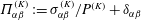 $\unicode[STIX]{x1D6F1}_{\unicode[STIX]{x1D6FC}\unicode[STIX]{x1D6FD}}^{(K)}:=\unicode[STIX]{x1D70E}_{\unicode[STIX]{x1D6FC}\unicode[STIX]{x1D6FD}}^{(K)}/P^{(K)}+\unicode[STIX]{x1D6FF}_{\unicode[STIX]{x1D6FC}\unicode[STIX]{x1D6FD}}$
is the normalized deviatoric stress, where
$\unicode[STIX]{x1D6F1}_{\unicode[STIX]{x1D6FC}\unicode[STIX]{x1D6FD}}^{(K)}:=\unicode[STIX]{x1D70E}_{\unicode[STIX]{x1D6FC}\unicode[STIX]{x1D6FD}}^{(K)}/P^{(K)}+\unicode[STIX]{x1D6FF}_{\unicode[STIX]{x1D6FC}\unicode[STIX]{x1D6FD}}$
is the normalized deviatoric stress, where
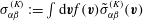 $\unicode[STIX]{x1D70E}_{\unicode[STIX]{x1D6FC}\unicode[STIX]{x1D6FD}}^{(K)}:=\int \text{d}\boldsymbol{v}f(\boldsymbol{v})\tilde{\unicode[STIX]{x1D70E}}_{\unicode[STIX]{x1D6FC}\unicode[STIX]{x1D6FD}}^{(K)}(\boldsymbol{v})$
and
$\unicode[STIX]{x1D70E}_{\unicode[STIX]{x1D6FC}\unicode[STIX]{x1D6FD}}^{(K)}:=\int \text{d}\boldsymbol{v}f(\boldsymbol{v})\tilde{\unicode[STIX]{x1D70E}}_{\unicode[STIX]{x1D6FC}\unicode[STIX]{x1D6FD}}^{(K)}(\boldsymbol{v})$
and
 $P^{(K)}:=-\unicode[STIX]{x1D70E}_{\unicode[STIX]{x1D6FC}\unicode[STIX]{x1D6FC}}^{(K)}/3$
are the macroscopic kinetic stress and the pressure,
$P^{(K)}:=-\unicode[STIX]{x1D70E}_{\unicode[STIX]{x1D6FC}\unicode[STIX]{x1D6FC}}^{(K)}/3$
are the macroscopic kinetic stress and the pressure,
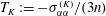 $T_{K}:=-\unicode[STIX]{x1D70E}_{\unicode[STIX]{x1D6FC}\unicode[STIX]{x1D6FC}}^{(K)}/(3n)$
is the kinetic temperature, where
$T_{K}:=-\unicode[STIX]{x1D70E}_{\unicode[STIX]{x1D6FC}\unicode[STIX]{x1D6FC}}^{(K)}/(3n)$
is the kinetic temperature, where
 $n$
is the average number density, and
$n$
is the average number density, and
 $f_{eq}(\boldsymbol{v})$
is the equilibrium distribution function. Note that the kinetic pressure satisfies the relation
$f_{eq}(\boldsymbol{v})$
is the equilibrium distribution function. Note that the kinetic pressure satisfies the relation
 $P^{(K)}=nT_{K}$
. This distribution function gives reasonably precise description of non-equilibrium gases, e.g. continuous as well as discontinuous shear thickening (Chamorro et al.
Reference Chamorro, Reyes and Garzó2015; Hayakawa & Takada Reference Hayakawa and Takada2016, Reference Hayakawa and Takada2017; Hayakawa et al.
Reference Hayakawa, Takada and Garzó2017). It is also notable that (4.6) satisfies the Green–Kubo formula within the Bhatnagar–Gross–Krook (BGK) approximation (Hayakawa & Takada Reference Hayakawa and Takada2016), while it further incorporates the normal stress differences, which is not the case for the Green–Kubo formula.
$P^{(K)}=nT_{K}$
. This distribution function gives reasonably precise description of non-equilibrium gases, e.g. continuous as well as discontinuous shear thickening (Chamorro et al.
Reference Chamorro, Reyes and Garzó2015; Hayakawa & Takada Reference Hayakawa and Takada2016, Reference Hayakawa and Takada2017; Hayakawa et al.
Reference Hayakawa, Takada and Garzó2017). It is also notable that (4.6) satisfies the Green–Kubo formula within the Bhatnagar–Gross–Krook (BGK) approximation (Hayakawa & Takada Reference Hayakawa and Takada2016), while it further incorporates the normal stress differences, which is not the case for the Green–Kubo formula.
The distribution function (4.6) cannot be directly applied to dense non-Brownian suspensions, where the Cauchy stress dominates the kinetic stress. A possible extension of this expansion for non-Brownian suspensions would be
 $$\begin{eqnarray}\displaystyle f(\unicode[STIX]{x1D71E},t)\approx f_{eq}(\unicode[STIX]{x1D71E}_{v})f_{eq}(\unicode[STIX]{x1D71E}_{r})\left[1+\frac{V}{2T}\unicode[STIX]{x1D6F1}_{\unicode[STIX]{x1D6FC}\unicode[STIX]{x1D6FD}}(t)\tilde{\unicode[STIX]{x1D70E}}_{\unicode[STIX]{x1D6FC}\unicode[STIX]{x1D6FD}}(\unicode[STIX]{x1D71E}_{r})\right], & & \displaystyle\end{eqnarray}$$
where
 $\unicode[STIX]{x1D71E}:=\{\unicode[STIX]{x1D71E}_{r},\unicode[STIX]{x1D71E}_{v}\}$
with
$\unicode[STIX]{x1D71E}:=\{\unicode[STIX]{x1D71E}_{r},\unicode[STIX]{x1D71E}_{v}\}$
with
 $\unicode[STIX]{x1D71E}_{r}:=\{\boldsymbol{r}_{i}\}\text{}_{i=1}^{N}$
and
$\unicode[STIX]{x1D71E}_{r}:=\{\boldsymbol{r}_{i}\}\text{}_{i=1}^{N}$
and
 $\unicode[STIX]{x1D71E}_{v}:=\{\boldsymbol{v}_{i}\}\text{}_{i=1}^{N}$
, and the kinetic stress is replaced by the Cauchy stress. Here,
$\unicode[STIX]{x1D71E}_{v}:=\{\boldsymbol{v}_{i}\}\text{}_{i=1}^{N}$
, and the kinetic stress is replaced by the Cauchy stress. Here,
 $$\begin{eqnarray}\displaystyle \unicode[STIX]{x1D6F1}_{\unicode[STIX]{x1D6FC}\unicode[STIX]{x1D6FD}}:=\frac{\unicode[STIX]{x1D70E}_{\unicode[STIX]{x1D6FC}\unicode[STIX]{x1D6FD}}}{P}+\unicode[STIX]{x1D6FF}_{\unicode[STIX]{x1D6FC}\unicode[STIX]{x1D6FD}} & & \displaystyle\end{eqnarray}$$
is the normalized deviatoric stress and the appropriate definition of the temperature
 $T$
for non-Brownian suspensions will be discussed in § 4.4. Here it is postulated that the distribution function is factorized into peculiar velocity-dependent and position-dependent parts, where the peculiar velocity-dependent part can be approximated by Gaussian,
$T$
for non-Brownian suspensions will be discussed in § 4.4. Here it is postulated that the distribution function is factorized into peculiar velocity-dependent and position-dependent parts, where the peculiar velocity-dependent part can be approximated by Gaussian,
 $f_{eq}(\unicode[STIX]{x1D71E}_{v})$
, and the position-dependent part is approximated by an expansion around equilibrium,
$f_{eq}(\unicode[STIX]{x1D71E}_{v})$
, and the position-dependent part is approximated by an expansion around equilibrium,
 $f_{eq}(\unicode[STIX]{x1D71E}_{r})$
, with the stress current. This expansion around equilibrium is non-trivial for non-Brownian suspensions, where the equilibrium state is absent. Nonetheless, we will show in § 6 that the velocity distribution is nearly Gaussian and thus the factorization of (4.7) seems to be valid, and the expansion of the position distribution with the stress current is applicable for the evaluation of the stress.
$f_{eq}(\unicode[STIX]{x1D71E}_{r})$
, with the stress current. This expansion around equilibrium is non-trivial for non-Brownian suspensions, where the equilibrium state is absent. Nonetheless, we will show in § 6 that the velocity distribution is nearly Gaussian and thus the factorization of (4.7) seems to be valid, and the expansion of the position distribution with the stress current is applicable for the evaluation of the stress.
From (4.7), the macroscopic average of an arbitrary observable
 $A(\unicode[STIX]{x1D71E}_{r})$
which depends on
$A(\unicode[STIX]{x1D71E}_{r})$
which depends on
 $\unicode[STIX]{x1D71E}_{r}$
is given by
$\unicode[STIX]{x1D71E}_{r}$
is given by
 $$\begin{eqnarray}\langle A(\unicode[STIX]{x1D71E}_{r}(t))\rangle \approx \langle A(\unicode[STIX]{x1D71E}_{r})\rangle _{eq}+\frac{V}{2T}\unicode[STIX]{x1D6F1}_{\unicode[STIX]{x1D6FC}\unicode[STIX]{x1D6FD}}(t)\langle A(\unicode[STIX]{x1D71E}_{r})\tilde{\unicode[STIX]{x1D70E}}_{\unicode[STIX]{x1D6FC}\unicode[STIX]{x1D6FD}}(\unicode[STIX]{x1D71E}_{r})\rangle _{eq},\end{eqnarray}$$
where the first term on the right-hand side is the canonical term with
 $$\begin{eqnarray}\displaystyle \langle \cdots \rangle _{eq}:=\int \text{d}\unicode[STIX]{x1D71E}_{r}f_{eq}(\unicode[STIX]{x1D71E}_{r})\cdots & & \displaystyle\end{eqnarray}$$
and the second term is its non-canonical correction. Note that (4.9) is formally equivalent to the multiple relaxation-time approximation of the Green–Kubo formula (Suzuki & Hayakawa Reference Suzuki and Hayakawa2015), where the dimensionless tensor
 $\unicode[STIX]{x1D6F1}_{\unicode[STIX]{x1D6FC}\unicode[STIX]{x1D6FD}}$
plays the role of the multiple relaxation times.
$\unicode[STIX]{x1D6F1}_{\unicode[STIX]{x1D6FC}\unicode[STIX]{x1D6FD}}$
plays the role of the multiple relaxation times.
4.2 Approximate expressions
Let us evaluate the two averages on the right-hand side of (4.5) via the approximate formula (4.9). Detailed evaluation of the averages is shown in § B.1. These two averages are written as sums of terms of the form
 $$\begin{eqnarray}\displaystyle \mathop{\sum }_{i=1}^{N}\mathop{\sum }_{j\neq i}\mathop{\sum }_{k\neq i}\langle X(\boldsymbol{r}_{ij})Y(\boldsymbol{r}_{ik})\rangle , & & \displaystyle\end{eqnarray}$$
where
 $X(\boldsymbol{r}_{ij})$
or
$X(\boldsymbol{r}_{ij})$
or
 $Y(\boldsymbol{r}_{ik})$
abbreviates term which depends on
$Y(\boldsymbol{r}_{ik})$
abbreviates term which depends on
 $\boldsymbol{r}_{ij}$
or
$\boldsymbol{r}_{ij}$
or
 $\boldsymbol{r}_{ik}$
, respectively. For instance, for the first term on the right-hand side (4.5),
$\boldsymbol{r}_{ik}$
, respectively. For instance, for the first term on the right-hand side (4.5),
 $X(\boldsymbol{r}_{ij})$
and
$X(\boldsymbol{r}_{ij})$
and
 $Y(\boldsymbol{r}_{ik})$
are given by
$Y(\boldsymbol{r}_{ik})$
are given by
 $X(\boldsymbol{r}_{ij})=\hat{r}_{ij,\unicode[STIX]{x1D6FC}}\unicode[STIX]{x1D6E5}_{ij}^{xy},Y(\boldsymbol{r}_{ik})=\hat{r}_{ik,\unicode[STIX]{x1D6FD}}\unicode[STIX]{x1D6E5}_{ik}^{xy}$
, or
$X(\boldsymbol{r}_{ij})=\hat{r}_{ij,\unicode[STIX]{x1D6FC}}\unicode[STIX]{x1D6E5}_{ij}^{xy},Y(\boldsymbol{r}_{ik})=\hat{r}_{ik,\unicode[STIX]{x1D6FD}}\unicode[STIX]{x1D6E5}_{ik}^{xy}$
, or
 $X(\boldsymbol{r}_{ij})=\hat{r}_{ij,\unicode[STIX]{x1D6FD}}\unicode[STIX]{x1D6E5}_{ij}^{xy},Y(\boldsymbol{r}_{ik})=\hat{r}_{ik,\unicode[STIX]{x1D6FC}}\unicode[STIX]{x1D6E5}_{ik}^{xy}$
. Terms of the form (4.11) are evaluated by (4.9) as
$X(\boldsymbol{r}_{ij})=\hat{r}_{ij,\unicode[STIX]{x1D6FD}}\unicode[STIX]{x1D6E5}_{ij}^{xy},Y(\boldsymbol{r}_{ik})=\hat{r}_{ik,\unicode[STIX]{x1D6FC}}\unicode[STIX]{x1D6E5}_{ik}^{xy}$
. Terms of the form (4.11) are evaluated by (4.9) as
 $$\begin{eqnarray}\displaystyle & & \displaystyle \mathop{\sum }_{i=1}^{N}\mathop{\sum }_{j\neq i}\mathop{\sum }_{k\neq i}\langle X(\boldsymbol{r}_{ij})Y(\boldsymbol{r}_{ik})\rangle \nonumber\\ \displaystyle & & \displaystyle \quad =\mathop{\sum }_{i=1}^{N}\mathop{\sum }_{j\neq i}\mathop{\sum }_{k\neq i}\left\{\langle X(\boldsymbol{r}_{ij})Y(\boldsymbol{r}_{ik})\rangle _{eq}+\frac{V}{2T}\unicode[STIX]{x1D6F1}_{\unicode[STIX]{x1D70C}\unicode[STIX]{x1D70E}}\langle X(\boldsymbol{r}_{ij})Y(\boldsymbol{r}_{ik})\tilde{\unicode[STIX]{x1D70E}}_{\unicode[STIX]{x1D70C}\unicode[STIX]{x1D70E}}\rangle _{eq}\right\}.\end{eqnarray}$$
Note that
 $\tilde{\unicode[STIX]{x1D70E}}_{\unicode[STIX]{x1D70C}\unicode[STIX]{x1D70E}}$
depends on the relative coordinate, e.g.
$\tilde{\unicode[STIX]{x1D70E}}_{\unicode[STIX]{x1D70C}\unicode[STIX]{x1D70E}}$
depends on the relative coordinate, e.g.
 $\boldsymbol{r}_{lm}$
, but either
$\boldsymbol{r}_{lm}$
, but either
 $l$
or
$l$
or
 $m$
must be identical to e.g.
$m$
must be identical to e.g.
 $i$
; otherwise the correlation decouples and vanishes. Hence, the non-equilibrium term is given by
$i$
; otherwise the correlation decouples and vanishes. Hence, the non-equilibrium term is given by
 $$\begin{eqnarray}\displaystyle \mathop{\sum }_{i=1}^{N}\mathop{\sum }_{j\neq i}\mathop{\sum }_{k\neq i}\mathop{\sum }_{l\neq i}\langle X(\boldsymbol{r}_{ij})Y(\boldsymbol{r}_{ik})\tilde{\unicode[STIX]{x1D70E}}_{\unicode[STIX]{x1D70C}\unicode[STIX]{x1D70E}}(\boldsymbol{r}_{il})\rangle _{eq}, & & \displaystyle\end{eqnarray}$$
which can be decomposed into four-, three- and two-body correlations as
 $$\begin{eqnarray}\displaystyle & & \displaystyle \mathop{\sum }_{i=1}^{N}\mathop{\sum }_{j\neq i}\mathop{\sum }_{k\neq i}\mathop{\sum }_{l\neq i}\langle X(\boldsymbol{r}_{ij})Y(\boldsymbol{r}_{ik})\tilde{\unicode[STIX]{x1D70E}}_{\unicode[STIX]{x1D70C}\unicode[STIX]{x1D70E}}(\boldsymbol{r}_{il})\rangle _{eq}=\sum _{i,j,k,l}\langle X(\boldsymbol{r}_{ij})Y(\boldsymbol{r}_{ik})\tilde{\unicode[STIX]{x1D70E}}_{\unicode[STIX]{x1D70C}\unicode[STIX]{x1D70E}}(\boldsymbol{r}_{il})\rangle _{eq}\nonumber\\ \displaystyle & & \displaystyle \quad +\,\sum _{i,j,k}\langle X(\boldsymbol{r}_{ij})Y(\boldsymbol{r}_{ik})\tilde{\unicode[STIX]{x1D70E}}_{\unicode[STIX]{x1D70C}\unicode[STIX]{x1D70E}}(\boldsymbol{r}_{ik})\rangle _{eq}+\sum _{i,j}\langle X(\boldsymbol{r}_{ij})Y(\boldsymbol{r}_{ij})\tilde{\unicode[STIX]{x1D70E}}_{\unicode[STIX]{x1D70C}\unicode[STIX]{x1D70E}}(\boldsymbol{r}_{ij})\rangle _{eq}.\end{eqnarray}$$
Here, the four-, three- and two-body terms are given by
 $$\begin{eqnarray}\displaystyle & \displaystyle \sum _{i,j,k,l}\langle X(\boldsymbol{r}_{ij})Y(\boldsymbol{r}_{ik})\tilde{\unicode[STIX]{x1D70E}}_{\unicode[STIX]{x1D70C}\unicode[STIX]{x1D70E}}(\boldsymbol{r}_{il})\rangle _{eq}=Nn^{3}\int \text{d}^{3}\boldsymbol{r}\int \text{d}^{3}\boldsymbol{r}^{\prime }\int \text{d}^{3}\boldsymbol{r}^{\prime \prime }g^{(4)}(\boldsymbol{r},\boldsymbol{r}^{\prime },\boldsymbol{r}^{\prime \prime })X(\boldsymbol{r})Y(\boldsymbol{r}^{\prime })\tilde{\unicode[STIX]{x1D70E}}_{\unicode[STIX]{x1D70C}\unicode[STIX]{x1D70E}}(\boldsymbol{r}^{\prime \prime }), & \displaystyle \nonumber\\ \displaystyle & & \displaystyle\end{eqnarray}$$
 $$\begin{eqnarray}\displaystyle & \displaystyle \sum _{i,j,k}\langle X(\boldsymbol{r}_{ij})Y(\boldsymbol{r}_{ik})\tilde{\unicode[STIX]{x1D70E}}_{\unicode[STIX]{x1D70C}\unicode[STIX]{x1D70E}}(\boldsymbol{r}_{ik})\rangle _{eq}=Nn^{3}\int \text{d}^{3}\boldsymbol{r}\int \text{d}^{3}\boldsymbol{r}^{\prime }g^{(3)}(\boldsymbol{r},\boldsymbol{r}^{\prime })X(\boldsymbol{r})Y(\boldsymbol{r}^{\prime })\tilde{\unicode[STIX]{x1D70E}}_{\unicode[STIX]{x1D70C}\unicode[STIX]{x1D70E}}(\boldsymbol{r}^{\prime }), & \displaystyle\end{eqnarray}$$
 $$\begin{eqnarray}\displaystyle & \displaystyle \sum _{i,j(i\neq j)}\langle X(\boldsymbol{r}_{ij})Y(\boldsymbol{r}_{ij})\tilde{\unicode[STIX]{x1D70E}}_{\unicode[STIX]{x1D70C}\unicode[STIX]{x1D70E}}(\boldsymbol{r}_{ij})\rangle _{eq}=Nn^{3}\int \text{d}^{3}\boldsymbol{r}g(r)X(\boldsymbol{r})Y(\boldsymbol{r})\tilde{\unicode[STIX]{x1D70E}}_{\unicode[STIX]{x1D70C}\unicode[STIX]{x1D70E}}(\boldsymbol{r}), & \displaystyle\end{eqnarray}$$
respectively, where
 $g^{(4)}(\boldsymbol{r},\boldsymbol{r}^{\prime },\boldsymbol{r}^{\prime \prime })$
and
$g^{(4)}(\boldsymbol{r},\boldsymbol{r}^{\prime },\boldsymbol{r}^{\prime \prime })$
and
 $g^{(3)}(\boldsymbol{r},\boldsymbol{r}^{\prime })$
are the quadruplet-correlation function (Hansen & McDonald Reference Hansen and McDonald2006)
$g^{(3)}(\boldsymbol{r},\boldsymbol{r}^{\prime })$
are the quadruplet-correlation function (Hansen & McDonald Reference Hansen and McDonald2006)
 $$\begin{eqnarray}g^{(4)}(\boldsymbol{r},\boldsymbol{r}^{\prime },\boldsymbol{r}^{\prime \prime }):=\frac{1}{Nn^{3}}\sum _{i,j,k,l}\langle \unicode[STIX]{x1D6FF}(\boldsymbol{r}-\boldsymbol{r}_{ij})\unicode[STIX]{x1D6FF}(\boldsymbol{r}^{\prime }-\boldsymbol{r}_{ik})\unicode[STIX]{x1D6FF}(\boldsymbol{r}^{\prime \prime }-\boldsymbol{r}_{il})\rangle _{eq}\end{eqnarray}$$
and the triplet-correlation function (Hansen & McDonald Reference Hansen and McDonald2006)
 $$\begin{eqnarray}g^{(3)}(\boldsymbol{r},\boldsymbol{r}^{\prime }):=\frac{1}{Nn^{2}}\sum _{i,j,k}\langle \unicode[STIX]{x1D6FF}(\boldsymbol{r}-\boldsymbol{r}_{ij})\unicode[STIX]{x1D6FF}(\boldsymbol{r}^{\prime }-\boldsymbol{r}_{ik})\rangle _{eq},\end{eqnarray}$$
and the summations
 $\sum _{i,j,k}^{\prime \prime }$
, and
$\sum _{i,j,k}^{\prime \prime }$
, and
 $\sum _{i,j,k,l}^{\prime \prime \prime }$
are performed over different particles. For instance,
$\sum _{i,j,k,l}^{\prime \prime \prime }$
are performed over different particles. For instance,
 $\sum _{i,j,k}^{\prime \prime }$
is performed for
$\sum _{i,j,k}^{\prime \prime }$
is performed for
 $i,j,k$
with
$i,j,k$
with
 $i\neq j$
,
$i\neq j$
,
 $j\neq k$
and
$j\neq k$
and
 $k\neq i$
. In the spatial integrations over
$k\neq i$
. In the spatial integrations over
 $g(r)$
,
$g(r)$
,
 $g^{(3)}(\boldsymbol{r},\boldsymbol{r}^{\prime })$
, or
$g^{(3)}(\boldsymbol{r},\boldsymbol{r}^{\prime })$
, or
 $g^{(4)}(\boldsymbol{r},\boldsymbol{r}^{\prime },\boldsymbol{r}^{\prime \prime })$
, it is crucial that these correlation functions are accompanied by the delta functions
$g^{(4)}(\boldsymbol{r},\boldsymbol{r}^{\prime },\boldsymbol{r}^{\prime \prime })$
, it is crucial that these correlation functions are accompanied by the delta functions
 $\unicode[STIX]{x1D6FF}(r-d)$
,
$\unicode[STIX]{x1D6FF}(r-d)$
,
 $\unicode[STIX]{x1D6FF}(r-d)\unicode[STIX]{x1D6FF}(r^{\prime }-d)$
, or
$\unicode[STIX]{x1D6FF}(r-d)\unicode[STIX]{x1D6FF}(r^{\prime }-d)$
, or
 $\unicode[STIX]{x1D6FF}(r-d)\unicode[STIX]{x1D6FF}(r^{\prime }-d)\unicode[STIX]{x1D6FF}(r^{\prime \prime }-d)$
, respectively. This feature can be explicitly traced back in (4.5), and is a consequence of the hard-core collision of the particles, equation (3.15). This implies that only the contact values of the correlation functions contribute. By virtue of this feature, we can conveniently approximate
$\unicode[STIX]{x1D6FF}(r-d)\unicode[STIX]{x1D6FF}(r^{\prime }-d)\unicode[STIX]{x1D6FF}(r^{\prime \prime }-d)$
, respectively. This feature can be explicitly traced back in (4.5), and is a consequence of the hard-core collision of the particles, equation (3.15). This implies that only the contact values of the correlation functions contribute. By virtue of this feature, we can conveniently approximate
 $g^{(3)}(\boldsymbol{r},\boldsymbol{r}^{\prime })$
and
$g^{(3)}(\boldsymbol{r},\boldsymbol{r}^{\prime })$
and
 $g^{(4)}(\boldsymbol{r},\boldsymbol{r}^{\prime },\boldsymbol{r}^{\prime \prime })$
.
$g^{(4)}(\boldsymbol{r},\boldsymbol{r}^{\prime },\boldsymbol{r}^{\prime \prime })$
.
Let us consider
 $g^{(3)}(\boldsymbol{r},\boldsymbol{r}^{\prime })$
for illustration. First of all, we adopt the factorization approximation (Kirkwood Reference Kirkwood1935),
$g^{(3)}(\boldsymbol{r},\boldsymbol{r}^{\prime })$
for illustration. First of all, we adopt the factorization approximation (Kirkwood Reference Kirkwood1935),
 $g^{(3)}(\boldsymbol{r},\boldsymbol{r}^{\prime })\approx g(r)g(r^{\prime })g(|\boldsymbol{r}-\boldsymbol{r}^{\prime }|)$
. Although this approximation is not accurate in general, it has been argued that it is valid at contacts, where
$g^{(3)}(\boldsymbol{r},\boldsymbol{r}^{\prime })\approx g(r)g(r^{\prime })g(|\boldsymbol{r}-\boldsymbol{r}^{\prime }|)$
. Although this approximation is not accurate in general, it has been argued that it is valid at contacts, where
 $r,r^{\prime },|\boldsymbol{r}-\boldsymbol{r}^{\prime }|\approx d$
(Alder Reference Alder1964; Grouba, Zorin & Sevastianov Reference Grouba, Zorin and Sevastianov2004). Furthermore, we have shown in Suzuki & Hayakawa (Reference Suzuki and Hayakawa2015) that only the radial contacts contribute to the divergence in the vicinity of the jamming point, i.e.
$r,r^{\prime },|\boldsymbol{r}-\boldsymbol{r}^{\prime }|\approx d$
(Alder Reference Alder1964; Grouba, Zorin & Sevastianov Reference Grouba, Zorin and Sevastianov2004). Furthermore, we have shown in Suzuki & Hayakawa (Reference Suzuki and Hayakawa2015) that only the radial contacts contribute to the divergence in the vicinity of the jamming point, i.e.
 $$\begin{eqnarray}\displaystyle g^{(3)}(\boldsymbol{r},\boldsymbol{r}^{\prime })\approx g(r)g(r^{\prime }) & & \displaystyle\end{eqnarray}$$
for
 $r,r^{\prime }\approx d$
. Similarly,
$r,r^{\prime }\approx d$
. Similarly,
 $g^{(4)}(\boldsymbol{r},\boldsymbol{r}^{\prime },\boldsymbol{r}^{\prime \prime })$
can be approximated as
$g^{(4)}(\boldsymbol{r},\boldsymbol{r}^{\prime },\boldsymbol{r}^{\prime \prime })$
can be approximated as
 $$\begin{eqnarray}\displaystyle g^{(4)}(\boldsymbol{r},\boldsymbol{r}^{\prime },\boldsymbol{r}^{\prime \prime })\approx g(r)g(r^{\prime })g(r^{\prime \prime })g(|\boldsymbol{r}-\boldsymbol{r}^{\prime }|)g(|\boldsymbol{r}^{\prime }-\boldsymbol{r}^{\prime \prime }|)g(|\boldsymbol{r}^{\prime \prime }-\boldsymbol{r}|)\approx g(r)g(r^{\prime })g(r^{\prime \prime })\qquad & & \displaystyle\end{eqnarray}$$
for
 $r,r^{\prime },r^{\prime \prime }\approx d$
, as far as divergence is concerned. We will examine the validity of the factorization approximation for the evaluation of the stress in § 6.
$r,r^{\prime },r^{\prime \prime }\approx d$
, as far as divergence is concerned. We will examine the validity of the factorization approximation for the evaluation of the stress in § 6.
These approximations, together with
 $g(r)\unicode[STIX]{x1D6FF}(r-d)=g_{0}(\unicode[STIX]{x1D711})\unicode[STIX]{x1D6FF}(r-d)$
, enable us to express the two averages on the right-hand side of (4.5) in terms of polynomials of the radial distribution function at contact,
$g(r)\unicode[STIX]{x1D6FF}(r-d)=g_{0}(\unicode[STIX]{x1D711})\unicode[STIX]{x1D6FF}(r-d)$
, enable us to express the two averages on the right-hand side of (4.5) in terms of polynomials of the radial distribution function at contact,
 $g_{0}(\unicode[STIX]{x1D711})$
. From tedious but straightforward calculation as shown in §§ B.1 and B.2, we reach the approximate equation of the stress
$g_{0}(\unicode[STIX]{x1D711})$
. From tedious but straightforward calculation as shown in §§ B.1 and B.2, we reach the approximate equation of the stress
 $$\begin{eqnarray}\displaystyle & & \displaystyle \frac{\text{d}}{\text{d}t}\unicode[STIX]{x1D70E}_{\unicode[STIX]{x1D6FC}\unicode[STIX]{x1D6FD}}+\frac{1}{2}\dot{\unicode[STIX]{x1D6FE}}(\unicode[STIX]{x1D6FF}_{\unicode[STIX]{x1D6FC}x}\unicode[STIX]{x1D70E}_{y\unicode[STIX]{x1D6FD}}+\unicode[STIX]{x1D6FF}_{\unicode[STIX]{x1D6FD}x}\unicode[STIX]{x1D70E}_{y\unicode[STIX]{x1D6FC}})\approx \frac{\unicode[STIX]{x1D701}\dot{\unicode[STIX]{x1D6FE}}^{2}}{4d}\mathop{\sum }_{\ell =1}^{2}\{\!-\unicode[STIX]{x1D711}^{\ast 3}g_{0}(\unicode[STIX]{x1D711})^{2}{\mathcal{S}}_{\unicode[STIX]{x1D6FC}\unicode[STIX]{x1D6FD}}^{(\ell :c2)}-\unicode[STIX]{x1D711}^{\ast 2}g_{0}(\unicode[STIX]{x1D711}){\mathcal{S}}_{\unicode[STIX]{x1D6FC}\unicode[STIX]{x1D6FD}}^{(\ell :c1)}\nonumber\\ \displaystyle & & \displaystyle \quad +\,\unicode[STIX]{x1D6EC}\unicode[STIX]{x1D6F1}_{\unicode[STIX]{x1D70C}\unicode[STIX]{x1D706}}[\unicode[STIX]{x1D711}^{\ast 4}g_{0}(\unicode[STIX]{x1D711})^{3}{\mathcal{S}}_{\unicode[STIX]{x1D6FC}\unicode[STIX]{x1D6FD}\unicode[STIX]{x1D70C}\unicode[STIX]{x1D706}}^{(\ell :nc3)}+\unicode[STIX]{x1D711}^{\ast 3}g_{0}(\unicode[STIX]{x1D711})^{2}{\mathcal{S}}_{\unicode[STIX]{x1D6FC}\unicode[STIX]{x1D6FD}\unicode[STIX]{x1D70C}\unicode[STIX]{x1D706}}^{(\ell :nc2)}+\unicode[STIX]{x1D711}^{\ast 2}g_{0}(\unicode[STIX]{x1D711}){\mathcal{S}}_{\unicode[STIX]{x1D6FC}\unicode[STIX]{x1D6FD}\unicode[STIX]{x1D70C}\unicode[STIX]{x1D706}}^{(\ell :nc1)}]\!\},\end{eqnarray}$$
where the two terms with coefficients
 ${\mathcal{S}}_{\unicode[STIX]{x1D6FC}\unicode[STIX]{x1D6FD}}^{(\ell :c2)}$
and
${\mathcal{S}}_{\unicode[STIX]{x1D6FC}\unicode[STIX]{x1D6FD}}^{(\ell :c2)}$
and
 ${\mathcal{S}}_{\unicode[STIX]{x1D6FC}\unicode[STIX]{x1D6FD}}^{(\ell :c1)}$
are the canonical contributions, and the three terms with coefficients
${\mathcal{S}}_{\unicode[STIX]{x1D6FC}\unicode[STIX]{x1D6FD}}^{(\ell :c1)}$
are the canonical contributions, and the three terms with coefficients
 ${\mathcal{S}}_{\unicode[STIX]{x1D6FC}\unicode[STIX]{x1D6FD}\unicode[STIX]{x1D70C}\unicode[STIX]{x1D706}}^{(\ell :nc3)}$
,
${\mathcal{S}}_{\unicode[STIX]{x1D6FC}\unicode[STIX]{x1D6FD}\unicode[STIX]{x1D70C}\unicode[STIX]{x1D706}}^{(\ell :nc3)}$
,
 ${\mathcal{S}}_{\unicode[STIX]{x1D6FC}\unicode[STIX]{x1D6FD}\unicode[STIX]{x1D70C}\unicode[STIX]{x1D706}}^{(\ell :nc2)}$
and
${\mathcal{S}}_{\unicode[STIX]{x1D6FC}\unicode[STIX]{x1D6FD}\unicode[STIX]{x1D70C}\unicode[STIX]{x1D706}}^{(\ell :nc2)}$
and
 ${\mathcal{S}}_{\unicode[STIX]{x1D6FC}\unicode[STIX]{x1D6FD}\unicode[STIX]{x1D70C}\unicode[STIX]{x1D706}}^{(\ell :nc1)}$
are the non-equilibrium corrections. The coefficients
${\mathcal{S}}_{\unicode[STIX]{x1D6FC}\unicode[STIX]{x1D6FD}\unicode[STIX]{x1D70C}\unicode[STIX]{x1D706}}^{(\ell :nc1)}$
are the non-equilibrium corrections. The coefficients
 ${\mathcal{S}}_{\unicode[STIX]{x1D6FC}\unicode[STIX]{x1D6FD}}^{(\ell :c1)}$
,
${\mathcal{S}}_{\unicode[STIX]{x1D6FC}\unicode[STIX]{x1D6FD}}^{(\ell :c1)}$
,
 ${\mathcal{S}}_{\unicode[STIX]{x1D6FC}\unicode[STIX]{x1D6FD}}^{(\ell :c2)}$
and
${\mathcal{S}}_{\unicode[STIX]{x1D6FC}\unicode[STIX]{x1D6FD}}^{(\ell :c2)}$
and
 ${\mathcal{S}}_{\unicode[STIX]{x1D6FC}\unicode[STIX]{x1D6FD}\unicode[STIX]{x1D70C}\unicode[STIX]{x1D706}}^{(\ell :nc3)}$
,
${\mathcal{S}}_{\unicode[STIX]{x1D6FC}\unicode[STIX]{x1D6FD}\unicode[STIX]{x1D70C}\unicode[STIX]{x1D706}}^{(\ell :nc3)}$
,
 ${\mathcal{S}}_{\unicode[STIX]{x1D6FC}\unicode[STIX]{x1D6FD}\unicode[STIX]{x1D70C}\unicode[STIX]{x1D706}}^{(\ell :nc2)}$
,
${\mathcal{S}}_{\unicode[STIX]{x1D6FC}\unicode[STIX]{x1D6FD}\unicode[STIX]{x1D70C}\unicode[STIX]{x1D706}}^{(\ell :nc2)}$
,
 ${\mathcal{S}}_{\unicode[STIX]{x1D6FC}\unicode[STIX]{x1D6FD}\unicode[STIX]{x1D70C}\unicode[STIX]{x1D706}}^{(\ell :nc1)}$
are numbers which arise from angular integrals. Here, we have introduced a dimensionless scalar
${\mathcal{S}}_{\unicode[STIX]{x1D6FC}\unicode[STIX]{x1D6FD}\unicode[STIX]{x1D70C}\unicode[STIX]{x1D706}}^{(\ell :nc1)}$
are numbers which arise from angular integrals. Here, we have introduced a dimensionless scalar
 $$\begin{eqnarray}\displaystyle \unicode[STIX]{x1D6EC}:=\frac{\unicode[STIX]{x1D701}\dot{\unicode[STIX]{x1D6FE}}d^{2}}{4T}, & & \displaystyle\end{eqnarray}$$
and
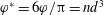 $\unicode[STIX]{x1D711}^{\ast }=6\unicode[STIX]{x1D711}/\unicode[STIX]{x03C0}=nd^{3}$
denotes the dimensionless number density.
$\unicode[STIX]{x1D711}^{\ast }=6\unicode[STIX]{x1D711}/\unicode[STIX]{x03C0}=nd^{3}$
denotes the dimensionless number density.
4.3 Implications of the symmetry
A specific feature of non-Brownian suspensions under simple shear is the symmetry under the parity ‘
 $\hat{x}\rightarrow -\hat{x}$
and
$\hat{x}\rightarrow -\hat{x}$
and
 ${\hat{y}}\rightarrow -{\hat{y}}$
’, which follows from
${\hat{y}}\rightarrow -{\hat{y}}$
’, which follows from
 ${\mathcal{P}}(\hat{x},{\hat{y}})$
introduced in (3.14). This implies that only the parity-even terms in (4.22) survive. Furthermore, even though parity even, terms odd with respect to
${\mathcal{P}}(\hat{x},{\hat{y}})$
introduced in (3.14). This implies that only the parity-even terms in (4.22) survive. Furthermore, even though parity even, terms odd with respect to
 $\hat{z}$
vanish. These features can be summarized as follows,
$\hat{z}$
vanish. These features can be summarized as follows,
 $$\begin{eqnarray}\displaystyle \int \text{d}{\mathcal{S}}\,\unicode[STIX]{x1D6E9}(-\hat{x}{\hat{y}})\hat{x}^{i}{\hat{y}}^{j}\hat{z}^{k}\neq 0\quad \text{if and only if }i+j=\text{even and }k=\text{even}, & & \displaystyle\end{eqnarray}$$
where
 $\int \text{d}{\mathcal{S}}\cdots \,$
expresses an angular integral with respect to
$\int \text{d}{\mathcal{S}}\cdots \,$
expresses an angular integral with respect to
 $\hat{\boldsymbol{r}}$
. As a consequence of this property we have
$\hat{\boldsymbol{r}}$
. As a consequence of this property we have
 $$\begin{eqnarray}\displaystyle \int \text{d}{\mathcal{S}}\unicode[STIX]{x1D6E9}(-\hat{x}{\hat{y}})\hat{x}^{i}{\hat{y}}^{j}\hat{z}^{k}=0\quad \text{if }i+j+k=\text{odd}. & & \displaystyle\end{eqnarray}$$
The terms proportional to
 $g_{0}(\unicode[STIX]{x1D711})^{3}$
in (4.22), which are cubic with respect to
$g_{0}(\unicode[STIX]{x1D711})^{3}$
in (4.22), which are cubic with respect to
 $\hat{\boldsymbol{r}}$
, vanish because of (4.25),
$\hat{\boldsymbol{r}}$
, vanish because of (4.25),
 $$\begin{eqnarray}\displaystyle {\mathcal{S}}_{\unicode[STIX]{x1D6FC}\unicode[STIX]{x1D6FD}\unicode[STIX]{x1D70C}\unicode[STIX]{x1D706}}^{(1:nc3)}={\mathcal{S}}_{\unicode[STIX]{x1D6FC}\unicode[STIX]{x1D6FD}\unicode[STIX]{x1D70C}\unicode[STIX]{x1D706}}^{(2:nc3)}=0. & & \displaystyle\end{eqnarray}$$
The same observation holds for the canonical terms proportional to
 $g_{0}(\unicode[STIX]{x1D711})^{2}$
, which are also cubic in
$g_{0}(\unicode[STIX]{x1D711})^{2}$
, which are also cubic in
 $\hat{\boldsymbol{r}}$
,
$\hat{\boldsymbol{r}}$
,
 $$\begin{eqnarray}\displaystyle {\mathcal{S}}_{\unicode[STIX]{x1D6FC}\unicode[STIX]{x1D6FD}}^{(1:c2)}={\mathcal{S}}_{\unicode[STIX]{x1D6FC}\unicode[STIX]{x1D6FD}}^{(2:c2)}=0. & & \displaystyle\end{eqnarray}$$
From (4.26) and (4.27), (4.22) reduces to
 $$\begin{eqnarray}\displaystyle & & \displaystyle \frac{\text{d}}{\text{d}t}\unicode[STIX]{x1D70E}_{\unicode[STIX]{x1D6FC}\unicode[STIX]{x1D6FD}}+\frac{1}{2}\dot{\unicode[STIX]{x1D6FE}}(\unicode[STIX]{x1D6FF}_{\unicode[STIX]{x1D6FC}x}\unicode[STIX]{x1D70E}_{y\unicode[STIX]{x1D6FD}}+\unicode[STIX]{x1D6FF}_{\unicode[STIX]{x1D6FD}x}\unicode[STIX]{x1D70E}_{y\unicode[STIX]{x1D6FC}})\approx \frac{\unicode[STIX]{x1D701}\dot{\unicode[STIX]{x1D6FE}}^{2}}{4d}\mathop{\sum }_{\ell =1}^{2}\{\!-\unicode[STIX]{x1D711}^{\ast 2}g_{0}(\unicode[STIX]{x1D711}){\mathcal{S}}_{\unicode[STIX]{x1D6FC}\unicode[STIX]{x1D6FD}}^{(\ell :c1)}\nonumber\\ \displaystyle & & \displaystyle \quad +\,\unicode[STIX]{x1D6EC}\unicode[STIX]{x1D6F1}_{\unicode[STIX]{x1D70C}\unicode[STIX]{x1D706}}[\unicode[STIX]{x1D711}^{\ast 3}g_{0}(\unicode[STIX]{x1D711})^{2}{\mathcal{S}}_{\unicode[STIX]{x1D6FC}\unicode[STIX]{x1D6FD}\unicode[STIX]{x1D70C}\unicode[STIX]{x1D706}}^{(\ell :nc2)}+\unicode[STIX]{x1D711}^{\ast 2}g_{0}(\unicode[STIX]{x1D711}){\mathcal{S}}_{\unicode[STIX]{x1D6FC}\unicode[STIX]{x1D6FD}\unicode[STIX]{x1D70C}\unicode[STIX]{x1D706}}^{(\ell :nc1)}]\!\},\end{eqnarray}$$
or, explicitly in components,
 $$\begin{eqnarray}\displaystyle \frac{\text{d}}{\text{d}t}\left(\begin{array}{@{}c@{}}\unicode[STIX]{x1D70E}_{xy}\\ -3P\\ \unicode[STIX]{x1D70E}_{xx}\\ \unicode[STIX]{x1D70E}_{yy}\end{array}\right)+\left(\begin{array}{@{}c@{}}\frac{1}{2}\unicode[STIX]{x1D70E}_{yy}\\ \unicode[STIX]{x1D70E}_{xy}\\ \unicode[STIX]{x1D70E}_{xy}\\ 0\end{array}\right)\approx \frac{\unicode[STIX]{x1D701}\dot{\unicode[STIX]{x1D6FE}}}{4d}\unicode[STIX]{x1D711}^{\ast 2}g_{0}(\unicode[STIX]{x1D711})\left\{-\boldsymbol{{\mathcal{B}}}+\unicode[STIX]{x1D6EC}(\unicode[STIX]{x1D711}^{\ast }g_{0}(\unicode[STIX]{x1D711})\boldsymbol{{\mathcal{A}}}^{(2)}+\boldsymbol{{\mathcal{A}}}^{(1)})\left(\begin{array}{@{}c@{}}\unicode[STIX]{x1D6F1}_{xy}\\ \unicode[STIX]{x1D6F1}_{xx}\\ \unicode[STIX]{x1D6F1}_{yy}\end{array}\right)\right\}, & & \displaystyle \nonumber\\ \displaystyle & & \displaystyle\end{eqnarray}$$
where the matrices
 $\boldsymbol{{\mathcal{A}}}^{(m)}$
(
$\boldsymbol{{\mathcal{A}}}^{(m)}$
(
 $m=1,2$
) and the vector
$m=1,2$
) and the vector
 $\boldsymbol{{\mathcal{B}}}$
are given by (C 64)–(C 66). Note that
$\boldsymbol{{\mathcal{B}}}$
are given by (C 64)–(C 66). Note that
 $\unicode[STIX]{x1D6F1}_{\unicode[STIX]{x1D6FC}\unicode[STIX]{x1D6FD}}$
is given by (4.8) and hence (4.29) is a closed set of equations for
$\unicode[STIX]{x1D6F1}_{\unicode[STIX]{x1D6FC}\unicode[STIX]{x1D6FD}}$
is given by (4.8) and hence (4.29) is a closed set of equations for
 $P$
,
$P$
,
 $\unicode[STIX]{x1D70E}_{xy}$
,
$\unicode[STIX]{x1D70E}_{xy}$
,
 $\unicode[STIX]{x1D70E}_{xx}$
and
$\unicode[STIX]{x1D70E}_{xx}$
and
 $\unicode[STIX]{x1D70E}_{yy}$
.
$\unicode[STIX]{x1D70E}_{yy}$
.
Note that (4.28) includes terms proportional to
 $g_{0}(\unicode[STIX]{x1D711})^{2}$
or
$g_{0}(\unicode[STIX]{x1D711})^{2}$
or
 $g_{0}(\unicode[STIX]{x1D711})$
. Hence, we decompose the stress tensor as
$g_{0}(\unicode[STIX]{x1D711})$
. Hence, we decompose the stress tensor as
 $\unicode[STIX]{x1D70E}_{\unicode[STIX]{x1D6FC}\unicode[STIX]{x1D6FD}}=\unicode[STIX]{x1D70E}_{\unicode[STIX]{x1D6FC}\unicode[STIX]{x1D6FD}}^{(2)}+\unicode[STIX]{x1D70E}_{\unicode[STIX]{x1D6FC}\unicode[STIX]{x1D6FD}}^{(1)}$
, where
$\unicode[STIX]{x1D70E}_{\unicode[STIX]{x1D6FC}\unicode[STIX]{x1D6FD}}=\unicode[STIX]{x1D70E}_{\unicode[STIX]{x1D6FC}\unicode[STIX]{x1D6FD}}^{(2)}+\unicode[STIX]{x1D70E}_{\unicode[STIX]{x1D6FC}\unicode[STIX]{x1D6FD}}^{(1)}$
, where
 $\unicode[STIX]{x1D70E}_{\unicode[STIX]{x1D6FC}\unicode[STIX]{x1D6FD}}^{(m)}$
is
$\unicode[STIX]{x1D70E}_{\unicode[STIX]{x1D6FC}\unicode[STIX]{x1D6FD}}^{(m)}$
is
 $O(g_{0}(\unicode[STIX]{x1D711})^{m})$
(
$O(g_{0}(\unicode[STIX]{x1D711})^{m})$
(
 $m=1,2$
), because (3.13) suggests that it is separable near the jamming point. Then, equation (4.28) is cast into two equations, each for
$m=1,2$
), because (3.13) suggests that it is separable near the jamming point. Then, equation (4.28) is cast into two equations, each for
 $\unicode[STIX]{x1D70E}_{\unicode[STIX]{x1D6FC}\unicode[STIX]{x1D6FD}}^{(2)}$
and
$\unicode[STIX]{x1D70E}_{\unicode[STIX]{x1D6FC}\unicode[STIX]{x1D6FD}}^{(2)}$
and
 $\unicode[STIX]{x1D70E}_{\unicode[STIX]{x1D6FC}\unicode[STIX]{x1D6FD}}^{(1)}$
, respectively,
$\unicode[STIX]{x1D70E}_{\unicode[STIX]{x1D6FC}\unicode[STIX]{x1D6FD}}^{(1)}$
, respectively,
 $$\begin{eqnarray}\displaystyle & \displaystyle \frac{\text{d}}{\text{d}t}\unicode[STIX]{x1D70E}_{\unicode[STIX]{x1D6FC}\unicode[STIX]{x1D6FD}}^{(2)}+\frac{1}{2}\dot{\unicode[STIX]{x1D6FE}}(\unicode[STIX]{x1D6FF}_{\unicode[STIX]{x1D6FC}x}\unicode[STIX]{x1D70E}_{\unicode[STIX]{x1D6FD}y}^{(2)}+\unicode[STIX]{x1D6FF}_{\unicode[STIX]{x1D6FD}x}\unicode[STIX]{x1D70E}_{\unicode[STIX]{x1D6FC}y}^{(2)})=\frac{\unicode[STIX]{x1D701}\dot{\unicode[STIX]{x1D6FE}}^{2}}{4d}\unicode[STIX]{x1D6EC}\unicode[STIX]{x1D711}^{\ast 3}g_{0}(\unicode[STIX]{x1D711})^{2}\unicode[STIX]{x1D6F1}_{\unicode[STIX]{x1D70C}\unicode[STIX]{x1D706}}^{(2)}\mathop{\sum }_{\ell =1}^{2}{\mathcal{S}}_{\unicode[STIX]{x1D6FC}\unicode[STIX]{x1D6FD}\unicode[STIX]{x1D70C}\unicode[STIX]{x1D706}}^{(\ell :nc2)}. & \displaystyle\end{eqnarray}$$
 $$\begin{eqnarray}\displaystyle & \displaystyle \frac{\text{d}}{\text{d}t}\unicode[STIX]{x1D70E}_{\unicode[STIX]{x1D6FC}\unicode[STIX]{x1D6FD}}^{(1)}+\frac{1}{2}\dot{\unicode[STIX]{x1D6FE}}(\unicode[STIX]{x1D6FF}_{\unicode[STIX]{x1D6FC}x}\unicode[STIX]{x1D70E}_{\unicode[STIX]{x1D6FD}y}^{(1)}+\unicode[STIX]{x1D6FF}_{\unicode[STIX]{x1D6FD}x}\unicode[STIX]{x1D70E}_{\unicode[STIX]{x1D6FC}y}^{(1)})=\frac{\unicode[STIX]{x1D701}\dot{\unicode[STIX]{x1D6FE}}^{2}}{4d}\unicode[STIX]{x1D711}^{\ast 2}g_{0}(\unicode[STIX]{x1D711})\mathop{\sum }_{\ell =1}^{2}\{-{\mathcal{S}}_{\unicode[STIX]{x1D6FC}\unicode[STIX]{x1D6FD}}^{(\ell :c1)}+\unicode[STIX]{x1D6EC}\unicode[STIX]{x1D6F1}_{\unicode[STIX]{x1D70C}\unicode[STIX]{x1D706}}^{(1)}{\mathcal{S}}_{\unicode[STIX]{x1D6FC}\unicode[STIX]{x1D6FD}\unicode[STIX]{x1D70C}\unicode[STIX]{x1D706}}^{(\ell :nc1)}\}.\qquad & \displaystyle\end{eqnarray}$$
Here, we have introduced
 $$\begin{eqnarray}\displaystyle \unicode[STIX]{x1D6F1}_{\unicode[STIX]{x1D6FC}\unicode[STIX]{x1D6FD}}^{(m)}:=\frac{\unicode[STIX]{x1D70E}_{\unicode[STIX]{x1D6FC}\unicode[STIX]{x1D6FD}}^{(m)}}{P^{(m)}}+\unicode[STIX]{x1D6FF}_{\unicode[STIX]{x1D6FC}\unicode[STIX]{x1D6FD}}\quad (m=1,2), & & \displaystyle\end{eqnarray}$$
where
 $P^{(m)}$
is the component of the pressure of
$P^{(m)}$
is the component of the pressure of
 $O(g_{0}(\unicode[STIX]{x1D711})^{m})$
(
$O(g_{0}(\unicode[STIX]{x1D711})^{m})$
(
 $m=1,2$
). The valid range of (4.30) and (4.31) from (4.28) is discussed in § D.2.
$m=1,2$
). The valid range of (4.30) and (4.31) from (4.28) is discussed in § D.2.
Another implication of the symmetry is that the uniform profile of the velocity distribution is maintained. This issue is discussed in appendix G.
4.4 Interpretation of the temperature
In contrast to the case of the kinetic theory of dilute and moderately dense gases, or even dense inertial suspensions near the jamming point, the determination method of the temperature
 $T$
is not clear for non-Brownian suspensions. As discussed in § 4.1, in the kinetic theory, the temperature is determined by the equation of state
$T$
is not clear for non-Brownian suspensions. As discussed in § 4.1, in the kinetic theory, the temperature is determined by the equation of state
 $P^{(K)}=nT_{K}$
, where
$P^{(K)}=nT_{K}$
, where
 $P^{(K)}$
and
$P^{(K)}$
and
 $T_{K}$
are the kinetic pressure and the kinetic temperature, respectively. We attempt to introduce the temperature by the Cauchy stress, which dominates the kinetic stress in dense non-Brownian suspensions. Because
$T_{K}$
are the kinetic pressure and the kinetic temperature, respectively. We attempt to introduce the temperature by the Cauchy stress, which dominates the kinetic stress in dense non-Brownian suspensions. Because
 $T$
appears in the position-dependent part in (4.7),
$T$
appears in the position-dependent part in (4.7),
 $T$
should be defined by the position-dependent Cauchy stress. Note that
$T$
should be defined by the position-dependent Cauchy stress. Note that
 $T$
determines the magnitude of the non-equilibrium correction of the distribution function, equation (4.7). Accordingly,
$T$
determines the magnitude of the non-equilibrium correction of the distribution function, equation (4.7). Accordingly,
 $\unicode[STIX]{x1D6EC}$
introduced in (4.23) determines the non-equilibrium correction of the stress, equations (4.28) or (4.29). In this paper, let us introduce
$\unicode[STIX]{x1D6EC}$
introduced in (4.23) determines the non-equilibrium correction of the stress, equations (4.28) or (4.29). In this paper, let us introduce
 $T$
by the equation of state
$T$
by the equation of state
 $$\begin{eqnarray}\displaystyle P^{(eq)}=nT[1+2\unicode[STIX]{x1D711}g_{0}(\unicode[STIX]{x1D711})], & & \displaystyle\end{eqnarray}$$
where
 $P^{(eq)}$
is the equilibrium part of the pressure determined from (4.28), (4.29) or (4.31) with
$P^{(eq)}$
is the equilibrium part of the pressure determined from (4.28), (4.29) or (4.31) with
 $\unicode[STIX]{x1D6EC}=0$
. In other words,
$\unicode[STIX]{x1D6EC}=0$
. In other words,
 $P^{(eq)}$
can be estimated only by
$P^{(eq)}$
can be estimated only by
 $f_{eq}(\unicode[STIX]{x1D71E}_{r})$
in (4.7). The solution of (4.31) is given in (D 2), (D 3) in § D.1, from which we obtain
$f_{eq}(\unicode[STIX]{x1D71E}_{r})$
in (4.7). The solution of (4.31) is given in (D 2), (D 3) in § D.1, from which we obtain
 $P^{(eq)}$
as (
$P^{(eq)}$
as (
 $P^{(1)}$
with
$P^{(1)}$
with
 $\unicode[STIX]{x1D6EC}=0$
)
$\unicode[STIX]{x1D6EC}=0$
)
 $$\begin{eqnarray}\displaystyle P^{(eq)}=0.0060\times \frac{\unicode[STIX]{x1D701}\dot{\unicode[STIX]{x1D6FE}}}{4d}\unicode[STIX]{x1D711}^{\ast 2}g_{0}(\unicode[STIX]{x1D711})=0.022\times \frac{\unicode[STIX]{x1D701}\dot{\unicode[STIX]{x1D6FE}}}{4d}\unicode[STIX]{x1D711}^{2}g_{0}(\unicode[STIX]{x1D711}), & & \displaystyle\end{eqnarray}$$
where
 $\unicode[STIX]{x1D711}^{\ast }=6\unicode[STIX]{x1D711}/\unicode[STIX]{x03C0}$
. Thus, from (4.33) and (4.34), we obtain
$\unicode[STIX]{x1D711}^{\ast }=6\unicode[STIX]{x1D711}/\unicode[STIX]{x03C0}$
. Thus, from (4.33) and (4.34), we obtain
 $$\begin{eqnarray}\displaystyle T=0.022\times \frac{\unicode[STIX]{x1D701}\dot{\unicode[STIX]{x1D6FE}}}{4nd}\frac{\unicode[STIX]{x1D711}^{2}g_{0}(\unicode[STIX]{x1D711})}{1+2\unicode[STIX]{x1D711}g_{0}(\unicode[STIX]{x1D711})}\approx 0.022\times \frac{\unicode[STIX]{x1D701}\dot{\unicode[STIX]{x1D6FE}}d^{2}}{8nd^{3}}\unicode[STIX]{x1D711}=0.0014\unicode[STIX]{x1D701}\dot{\unicode[STIX]{x1D6FE}}d^{2}, & & \displaystyle\end{eqnarray}$$
where we have approximated
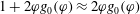 $1+2\unicode[STIX]{x1D711}g_{0}(\unicode[STIX]{x1D711})\approx 2\unicode[STIX]{x1D711}g_{0}(\unicode[STIX]{x1D711})$
in the second equality. This determines
$1+2\unicode[STIX]{x1D711}g_{0}(\unicode[STIX]{x1D711})\approx 2\unicode[STIX]{x1D711}g_{0}(\unicode[STIX]{x1D711})$
in the second equality. This determines
 $\unicode[STIX]{x1D6EC}$
as
$\unicode[STIX]{x1D6EC}$
as
 $$\begin{eqnarray}\displaystyle \unicode[STIX]{x1D6EC}=\frac{\unicode[STIX]{x1D701}\dot{\unicode[STIX]{x1D6FE}}d^{2}}{4T}\approx 174, & & \displaystyle\end{eqnarray}$$
which is independent of dimensional physical variables such as
 $\dot{\unicode[STIX]{x1D6FE}}$
,
$\dot{\unicode[STIX]{x1D6FE}}$
,
 $d$
or
$d$
or
 $\unicode[STIX]{x1D702}_{0}$
, and is merely a number. This value is larger than the value
$\unicode[STIX]{x1D702}_{0}$
, and is merely a number. This value is larger than the value
 $\unicode[STIX]{x1D6EC}=0.04$
determined by fitting the absolute values of the shear and pressure viscosities to the result of molecular dynamics (MD) simulation (cf. §§ 4.5 and 5). This might be due to the fact that
$\unicode[STIX]{x1D6EC}=0.04$
determined by fitting the absolute values of the shear and pressure viscosities to the result of molecular dynamics (MD) simulation (cf. §§ 4.5 and 5). This might be due to the fact that
 $\unicode[STIX]{x1D701}$
in (4.36) is not equivalent to
$\unicode[STIX]{x1D701}$
in (4.36) is not equivalent to
 $\unicode[STIX]{x1D701}_{0}$
which sets the magnitude of the viscosities in MD simulation. In fact,
$\unicode[STIX]{x1D701}_{0}$
which sets the magnitude of the viscosities in MD simulation. In fact,
 $\unicode[STIX]{x1D701}$
is given by (4.3) as
$\unicode[STIX]{x1D701}$
is given by (4.3) as
 $\unicode[STIX]{x1D701}=3\unicode[STIX]{x1D701}_{0}/(128\unicode[STIX]{x1D716}^{2})$
, where
$\unicode[STIX]{x1D701}=3\unicode[STIX]{x1D701}_{0}/(128\unicode[STIX]{x1D716}^{2})$
, where
 $\unicode[STIX]{x1D716}\ll 1$
is the magnitude of the separation of contacting particles. The ratio
$\unicode[STIX]{x1D716}\ll 1$
is the magnitude of the separation of contacting particles. The ratio
 $\unicode[STIX]{x1D701}/\unicode[STIX]{x1D701}_{0}=174/0.04$
corresponds to
$\unicode[STIX]{x1D701}/\unicode[STIX]{x1D701}_{0}=174/0.04$
corresponds to
 $\unicode[STIX]{x1D716}\approx 0.002$
, but since we cannot determine the magnitude of
$\unicode[STIX]{x1D716}\approx 0.002$
, but since we cannot determine the magnitude of
 $\unicode[STIX]{x1D716}$
in our framework, we will leave
$\unicode[STIX]{x1D716}$
in our framework, we will leave
 $\unicode[STIX]{x1D6EC}$
as a fitting parameter.
$\unicode[STIX]{x1D6EC}$
as a fitting parameter.
The important implication of (4.35) is
 $$\begin{eqnarray}\displaystyle T\propto \unicode[STIX]{x1D701}\dot{\unicode[STIX]{x1D6FE}}d^{2}\propto 3\unicode[STIX]{x03C0}d^{3}\unicode[STIX]{x1D702}_{0}\dot{\unicode[STIX]{x1D6FE}}, & & \displaystyle\end{eqnarray}$$
which is consistent with the ‘effective temperature’ of suspensions (Ono et al.
Reference Ono, O’Hern, Durian, Langer, Liu and Nagel2002; Eisenmann et al.
Reference Eisenmann, Kim, Mattsson and Weitz2010) defined via the Stokes–Einstein relation,
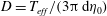 $D=T_{eff}/(3\unicode[STIX]{x03C0}\,\text{d}\unicode[STIX]{x1D702}_{0})$
, where
$D=T_{eff}/(3\unicode[STIX]{x03C0}\,\text{d}\unicode[STIX]{x1D702}_{0})$
, where
 $D$
is the diffusion coefficient. It has been shown by experiment (Leighton & Acrivos Reference Leighton and Acrivos1987a
,Reference Leighton and Acrivos
b
; Breedveld et al.
Reference Breedveld, van den Ende, Tripathi and Acrivos1998, Reference Breedveld, van den Ende, Bosscher, Jongschaap and Mellema2002; Eisenmann et al.
Reference Eisenmann, Kim, Mattsson and Weitz2010) and simulation (Foss & Brady Reference Foss and Brady1999; Heussinger et al.
Reference Heussinger, Berthier and Barrat2010; Olsson Reference Olsson2010) that
$D$
is the diffusion coefficient. It has been shown by experiment (Leighton & Acrivos Reference Leighton and Acrivos1987a
,Reference Leighton and Acrivos
b
; Breedveld et al.
Reference Breedveld, van den Ende, Tripathi and Acrivos1998, Reference Breedveld, van den Ende, Bosscher, Jongschaap and Mellema2002; Eisenmann et al.
Reference Eisenmann, Kim, Mattsson and Weitz2010) and simulation (Foss & Brady Reference Foss and Brady1999; Heussinger et al.
Reference Heussinger, Berthier and Barrat2010; Olsson Reference Olsson2010) that
 $D\sim \text{d}^{2}\dot{\unicode[STIX]{x1D6FE}}$
holds below the jamming point and
$D\sim \text{d}^{2}\dot{\unicode[STIX]{x1D6FE}}$
holds below the jamming point and
 $D$
exhibits only a weak dependence on the density, which suggests
$D$
exhibits only a weak dependence on the density, which suggests
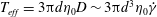 $T_{eff}=3\unicode[STIX]{x03C0}d\unicode[STIX]{x1D702}_{0}D\sim 3\unicode[STIX]{x03C0}d^{3}\unicode[STIX]{x1D702}_{0}\dot{\unicode[STIX]{x1D6FE}}$
.
$T_{eff}=3\unicode[STIX]{x03C0}d\unicode[STIX]{x1D702}_{0}D\sim 3\unicode[STIX]{x03C0}d^{3}\unicode[STIX]{x1D702}_{0}\dot{\unicode[STIX]{x1D6FE}}$
.
4.5 Viscosities and
$\unicode[STIX]{x1D707}$
–
$J$
rheology in the steady state


Let us analyse the rheology in the steady state, i.e. consider (4.28) with
 $\text{d}\unicode[STIX]{x1D70E}_{\unicode[STIX]{x1D6FC}\unicode[STIX]{x1D6FD}}/\text{d}t=0$
. Then, equations (4.30) and (4.31) can be solved analytically. The analytic solutions for
$\text{d}\unicode[STIX]{x1D70E}_{\unicode[STIX]{x1D6FC}\unicode[STIX]{x1D6FD}}/\text{d}t=0$
. Then, equations (4.30) and (4.31) can be solved analytically. The analytic solutions for
 $\unicode[STIX]{x1D70E}_{\unicode[STIX]{x1D6FC}\unicode[STIX]{x1D6FD}}^{(2)}$
and
$\unicode[STIX]{x1D70E}_{\unicode[STIX]{x1D6FC}\unicode[STIX]{x1D6FD}}^{(2)}$
and
 $\unicode[STIX]{x1D70E}_{\unicode[STIX]{x1D6FC}\unicode[STIX]{x1D6FD}}^{(1)}$
are given by (D 1)–(D 4) in § D.1, together with (3.13):
$\unicode[STIX]{x1D70E}_{\unicode[STIX]{x1D6FC}\unicode[STIX]{x1D6FD}}^{(1)}$
are given by (D 1)–(D 4) in § D.1, together with (3.13):
 $$\begin{eqnarray}\displaystyle & \displaystyle \unicode[STIX]{x1D70E}_{\unicode[STIX]{x1D6FC}\unicode[STIX]{x1D6FD}}^{(2)}\sim \frac{\unicode[STIX]{x1D701}\dot{\unicode[STIX]{x1D6FE}}}{d}g_{0}(\unicode[STIX]{x1D711})^{2}\sim \frac{\unicode[STIX]{x1D701}\dot{\unicode[STIX]{x1D6FE}}}{d}\unicode[STIX]{x1D6FF}\unicode[STIX]{x1D711}^{-2}, & \displaystyle\end{eqnarray}$$
 $$\begin{eqnarray}\displaystyle & \displaystyle \unicode[STIX]{x1D70E}_{\unicode[STIX]{x1D6FC}\unicode[STIX]{x1D6FD}}^{(1)}\sim \frac{\unicode[STIX]{x1D701}\dot{\unicode[STIX]{x1D6FE}}}{d}g_{0}(\unicode[STIX]{x1D711})\sim \frac{\unicode[STIX]{x1D701}\dot{\unicode[STIX]{x1D6FE}}}{d}\unicode[STIX]{x1D6FF}\unicode[STIX]{x1D711}^{-1}. & \displaystyle\end{eqnarray}$$
In particular, the normalized shear viscosity
 $\unicode[STIX]{x1D702}_{s}^{\ast }:=\unicode[STIX]{x1D702}_{s}/\unicode[STIX]{x1D702}_{0}$
and pressure viscosity
$\unicode[STIX]{x1D702}_{s}^{\ast }:=\unicode[STIX]{x1D702}_{s}/\unicode[STIX]{x1D702}_{0}$
and pressure viscosity
 $\unicode[STIX]{x1D702}_{n}^{\ast }:=\unicode[STIX]{x1D702}_{n}/\unicode[STIX]{x1D702}_{0}$
are given by
$\unicode[STIX]{x1D702}_{n}^{\ast }:=\unicode[STIX]{x1D702}_{n}/\unicode[STIX]{x1D702}_{0}$
are given by
 $$\begin{eqnarray}\displaystyle & \displaystyle \unicode[STIX]{x1D702}_{s}^{\ast }\approx 0.0073\unicode[STIX]{x1D711}^{\ast 3}\unicode[STIX]{x1D6FF}\unicode[STIX]{x1D711}^{-2}+0.080\unicode[STIX]{x1D711}^{\ast 2}\unicode[STIX]{x1D6FF}\unicode[STIX]{x1D711}^{-1}, & \displaystyle\end{eqnarray}$$
 $$\begin{eqnarray}\displaystyle & \displaystyle \unicode[STIX]{x1D702}_{n}^{\ast }\approx 0.045\unicode[STIX]{x1D711}^{\ast 3}\unicode[STIX]{x1D6FF}\unicode[STIX]{x1D711}^{-2}+0.0005\unicode[STIX]{x1D711}^{\ast 2}\unicode[STIX]{x1D6FF}\unicode[STIX]{x1D711}^{-1}\approx 0.045\unicode[STIX]{x1D711}^{\ast 3}\unicode[STIX]{x1D6FF}\unicode[STIX]{x1D711}^{-2}, & \displaystyle\end{eqnarray}$$
where
 $\unicode[STIX]{x1D6EC}=0.04$
is adopted, which is determined by fitting the absolute values of
$\unicode[STIX]{x1D6EC}=0.04$
is adopted, which is determined by fitting the absolute values of
 $\unicode[STIX]{x1D702}_{s}^{\ast }$
and
$\unicode[STIX]{x1D702}_{s}^{\ast }$
and
 $\unicode[STIX]{x1D702}_{n}^{\ast }$
to the results of the MD simulation shown in the next section. The empirical formula
$\unicode[STIX]{x1D702}_{n}^{\ast }$
to the results of the MD simulation shown in the next section. The empirical formula
 $g_{0}(\unicode[STIX]{x1D711})=g_{CS}(\unicode[STIX]{x1D711}_{f})(\unicode[STIX]{x1D711}_{J}-\unicode[STIX]{x1D711}_{f})/(\unicode[STIX]{x1D711}_{J}-\unicode[STIX]{x1D711})$
with
$g_{0}(\unicode[STIX]{x1D711})=g_{CS}(\unicode[STIX]{x1D711}_{f})(\unicode[STIX]{x1D711}_{J}-\unicode[STIX]{x1D711}_{f})/(\unicode[STIX]{x1D711}_{J}-\unicode[STIX]{x1D711})$
with
 $\unicode[STIX]{x1D711}_{f}=0.49$
and
$\unicode[STIX]{x1D711}_{f}=0.49$
and
 $g_{CS}(\unicode[STIX]{x1D711}):=(1-\unicode[STIX]{x1D711}/2)/(1-\unicode[STIX]{x1D711})^{3}$
valid for
$g_{CS}(\unicode[STIX]{x1D711}):=(1-\unicode[STIX]{x1D711}/2)/(1-\unicode[STIX]{x1D711})^{3}$
valid for
 $\unicode[STIX]{x1D711}_{f}<\unicode[STIX]{x1D711}<\unicode[STIX]{x1D711}_{J}$
(Torquato Reference Torquato1995) is adopted, from which we obtain
$\unicode[STIX]{x1D711}_{f}<\unicode[STIX]{x1D711}<\unicode[STIX]{x1D711}_{J}$
(Torquato Reference Torquato1995) is adopted, from which we obtain
 $g_{0}(\unicode[STIX]{x1D711})\approx 0.848\,\unicode[STIX]{x1D6FF}\unicode[STIX]{x1D711}^{-1}$
for
$g_{0}(\unicode[STIX]{x1D711})\approx 0.848\,\unicode[STIX]{x1D6FF}\unicode[STIX]{x1D711}^{-1}$
for
 $\unicode[STIX]{x1D711}_{J}=0.639$
. Although it is widely recognized that
$\unicode[STIX]{x1D711}_{J}=0.639$
. Although it is widely recognized that
 $\unicode[STIX]{x1D711}_{J}\approx 0.64$
for monodisperse frictionless hard spheres without any solvent, it has been reported that the value of
$\unicode[STIX]{x1D711}_{J}\approx 0.64$
for monodisperse frictionless hard spheres without any solvent, it has been reported that the value of
 $\unicode[STIX]{x1D711}_{J}$
is not uniquely identified and depends on the protocols used to generate the jammed configurations (Ciamarra, Coniglio & de Candia Reference Ciamarra, Coniglio and de Candia2010). In this work, we adopt
$\unicode[STIX]{x1D711}_{J}$
is not uniquely identified and depends on the protocols used to generate the jammed configurations (Ciamarra, Coniglio & de Candia Reference Ciamarra, Coniglio and de Candia2010). In this work, we adopt
 $\unicode[STIX]{x1D711}_{J}=0.639$
, which is obtained by the conjugate-gradient protocol (O’Hern et al.
Reference O’Hern, Silbert, Liu and Nagel2003). The numerical coefficients in (4.40) and (4.41) are determined analytically in rational forms, but we only show their approximate values in decimals for brevity.
$\unicode[STIX]{x1D711}_{J}=0.639$
, which is obtained by the conjugate-gradient protocol (O’Hern et al.
Reference O’Hern, Silbert, Liu and Nagel2003). The numerical coefficients in (4.40) and (4.41) are determined analytically in rational forms, but we only show their approximate values in decimals for brevity.
It is evident from (4.40) and (4.41) that
 $\unicode[STIX]{x1D702}_{s}^{\ast }$
and
$\unicode[STIX]{x1D702}_{s}^{\ast }$
and
 $\unicode[STIX]{x1D702}_{n}^{\ast }$
exhibit
$\unicode[STIX]{x1D702}_{n}^{\ast }$
exhibit
 $$\begin{eqnarray}\displaystyle \unicode[STIX]{x1D702}_{s}^{\ast }\sim \unicode[STIX]{x1D702}_{n}^{\ast }\sim \unicode[STIX]{x1D6FF}\unicode[STIX]{x1D711}^{-2} & & \displaystyle\end{eqnarray}$$
near the jamming point. On the other hand,
 $O(\unicode[STIX]{x1D6FF}\unicode[STIX]{x1D711}^{-1})$
term in
$O(\unicode[STIX]{x1D6FF}\unicode[STIX]{x1D711}^{-1})$
term in
 $\unicode[STIX]{x1D702}_{n}^{\ast }$
is small for finite
$\unicode[STIX]{x1D702}_{n}^{\ast }$
is small for finite
 $\unicode[STIX]{x1D6FF}\unicode[STIX]{x1D711}$
, while the corresponding term in
$\unicode[STIX]{x1D6FF}\unicode[STIX]{x1D711}$
, while the corresponding term in
 $\unicode[STIX]{x1D702}_{s}^{\ast }$
is significant. Noting
$\unicode[STIX]{x1D702}_{s}^{\ast }$
is significant. Noting
 $J=1/\unicode[STIX]{x1D702}_{n}^{\ast }$
,
$J=1/\unicode[STIX]{x1D702}_{n}^{\ast }$
,
 $J$
and
$J$
and
 $\unicode[STIX]{x1D6FF}\unicode[STIX]{x1D711}$
are uniquely invertible via (4.41) as
$\unicode[STIX]{x1D6FF}\unicode[STIX]{x1D711}$
are uniquely invertible via (4.41) as
 $$\begin{eqnarray}\displaystyle J^{1/2}\approx 4.74\unicode[STIX]{x1D711}^{\ast -3/2}\unicode[STIX]{x1D6FF}\unicode[STIX]{x1D711}, & & \displaystyle\end{eqnarray}$$
or, equivalently,
 $$\begin{eqnarray}\displaystyle \unicode[STIX]{x1D711}=\unicode[STIX]{x1D711}_{J}-0.211\unicode[STIX]{x1D711}^{\ast 3/2}J^{1/2}. & & \displaystyle\end{eqnarray}$$
From (4.40) and (4.41), we obtain the stress ratio
 $\unicode[STIX]{x1D707}$
as
$\unicode[STIX]{x1D707}$
as
 $$\begin{eqnarray}\displaystyle \unicode[STIX]{x1D707}\approx 0.163+1.78\unicode[STIX]{x1D711}^{\ast -1}\unicode[STIX]{x1D6FF}\unicode[STIX]{x1D711}=0.163+0.377\unicode[STIX]{x1D711}^{\ast 1/2}J^{1/2}. & & \displaystyle\end{eqnarray}$$
Note that
 $\unicode[STIX]{x1D707}$
in the jamming limit,
$\unicode[STIX]{x1D707}$
in the jamming limit,
 $\unicode[STIX]{x1D707}(J\rightarrow 0)=0.163$
, is independent of
$\unicode[STIX]{x1D707}(J\rightarrow 0)=0.163$
, is independent of
 $\unicode[STIX]{x1D6EC}$
.
$\unicode[STIX]{x1D6EC}$
.

Figure 3. Comparison of theory with MD simulation. (a) The normalized shear viscosity
 $\unicode[STIX]{x1D702}_{s}^{\ast }=\unicode[STIX]{x1D702}_{s}/\unicode[STIX]{x1D702}_{0}$
and the pressure viscosity
$\unicode[STIX]{x1D702}_{s}^{\ast }=\unicode[STIX]{x1D702}_{s}/\unicode[STIX]{x1D702}_{0}$
and the pressure viscosity
 $\unicode[STIX]{x1D702}_{n}^{\ast }=\unicode[STIX]{x1D702}_{n}/\unicode[STIX]{x1D702}_{0}$
, and (b) the stress ratio
$\unicode[STIX]{x1D702}_{n}^{\ast }=\unicode[STIX]{x1D702}_{n}/\unicode[STIX]{x1D702}_{0}$
, and (b) the stress ratio
 $\unicode[STIX]{x1D707}=\unicode[STIX]{x1D70E}_{xy}/P$
. The results of the theory and MD for the shear (pressure) viscosity are shown in dashed (solid) lines and open circles (squares) in (a), and those for the stress ratio are shown in solid line and open diamonds in (b), respectively. The theoretical result adopts the fitting parameter
$\unicode[STIX]{x1D707}=\unicode[STIX]{x1D70E}_{xy}/P$
. The results of the theory and MD for the shear (pressure) viscosity are shown in dashed (solid) lines and open circles (squares) in (a), and those for the stress ratio are shown in solid line and open diamonds in (b), respectively. The theoretical result adopts the fitting parameter
 $\unicode[STIX]{x1D6EC}=0.04$
. The result of MD is for
$\unicode[STIX]{x1D6EC}=0.04$
. The result of MD is for
 $\unicode[STIX]{x1D711}=$
0.632, 0.631, 0.63, 0.626, 0.62, 0.61, 0.6, 0.58, 0.54 and 0.5.
$\unicode[STIX]{x1D711}=$
0.632, 0.631, 0.63, 0.626, 0.62, 0.61, 0.6, 0.58, 0.54 and 0.5.
5 Comparison with simulation and previous results
We compare our theory with the MD simulation and previous results. We adopt the algorithm for Brownian hard spheres (Scala, Voigtmann & Michele Reference Scala, Voigtmann and Michele2007) applied at zero thermal fluctuations for the MD simulation. By this choice the only source of the velocity fluctuation is the interparticle contacts. The resistance matrix is simplified to
 $\overleftrightarrow{\unicode[STIX]{x1D701}^{(N)}}=\unicode[STIX]{x1D701}_{0}\unicode[STIX]{x1D644}$
, where
$\overleftrightarrow{\unicode[STIX]{x1D701}^{(N)}}=\unicode[STIX]{x1D701}_{0}\unicode[STIX]{x1D644}$
, where
 $\unicode[STIX]{x1D701}_{0}:=3\unicode[STIX]{x03C0}d\,\unicode[STIX]{x1D702}_{0}$
. The details of the simulation scheme is presented in appendix F.
$\unicode[STIX]{x1D701}_{0}:=3\unicode[STIX]{x03C0}d\,\unicode[STIX]{x1D702}_{0}$
. The details of the simulation scheme is presented in appendix F.
We show the results for the normalized shear viscosity
 $\unicode[STIX]{x1D702}_{s}^{\ast }$
, equation (4.40), pressure viscosity
$\unicode[STIX]{x1D702}_{s}^{\ast }$
, equation (4.40), pressure viscosity
 $\unicode[STIX]{x1D702}_{n}^{\ast }$
, equation (4.41) and the stress ratio
$\unicode[STIX]{x1D702}_{n}^{\ast }$
, equation (4.41) and the stress ratio
 $\unicode[STIX]{x1D707}$
, equation (4.45), in figure 3. As is already mentioned, we adopt
$\unicode[STIX]{x1D707}$
, equation (4.45), in figure 3. As is already mentioned, we adopt
 $\unicode[STIX]{x1D6EC}=0.04$
as a fitting parameter for
$\unicode[STIX]{x1D6EC}=0.04$
as a fitting parameter for
 $\unicode[STIX]{x1D702}_{s}^{\ast }$
and
$\unicode[STIX]{x1D702}_{s}^{\ast }$
and
 $\unicode[STIX]{x1D702}_{n}^{\ast }$
. In the dense region, the theory predicts
$\unicode[STIX]{x1D702}_{n}^{\ast }$
. In the dense region, the theory predicts
 $\unicode[STIX]{x1D702}_{s}^{\ast }\sim \unicode[STIX]{x1D702}_{n}^{\ast }\sim \unicode[STIX]{x1D6FF}\unicode[STIX]{x1D711}^{-2}$
in accordance with the MD result, and the stress ratio approaches
$\unicode[STIX]{x1D702}_{s}^{\ast }\sim \unicode[STIX]{x1D702}_{n}^{\ast }\sim \unicode[STIX]{x1D6FF}\unicode[STIX]{x1D711}^{-2}$
in accordance with the MD result, and the stress ratio approaches
 $\unicode[STIX]{x1D707}(J\rightarrow 0)=0.163$
, which is also in good agreement with MD. Because there exists slight difference between
$\unicode[STIX]{x1D707}(J\rightarrow 0)=0.163$
, which is also in good agreement with MD. Because there exists slight difference between
 $\unicode[STIX]{x1D702}_{s}^{\ast }$
and
$\unicode[STIX]{x1D702}_{s}^{\ast }$
and
 $\unicode[STIX]{x1D702}_{n}^{\ast }$
for finite
$\unicode[STIX]{x1D702}_{n}^{\ast }$
for finite
 $\unicode[STIX]{x1D6FF}\unicode[STIX]{x1D711}$
, we find that
$\unicode[STIX]{x1D6FF}\unicode[STIX]{x1D711}$
, we find that
 $\unicode[STIX]{x1D707}$
depends on
$\unicode[STIX]{x1D707}$
depends on
 $J$
or
$J$
or
 $\unicode[STIX]{x1D6FF}\unicode[STIX]{x1D711}$
(
$\unicode[STIX]{x1D6FF}\unicode[STIX]{x1D711}$
(
 $\unicode[STIX]{x1D707}$
–
$\unicode[STIX]{x1D707}$
–
 $J$
rheology). A reasonable agreement between our theory and MD is found, although the applicability for large
$J$
rheology). A reasonable agreement between our theory and MD is found, although the applicability for large
 $J$
in our theory is questionable (see § D.2).
$J$
in our theory is questionable (see § D.2).
We compare our theory with previous results. It is notable that (4.43) and (4.45) are consistent with the experimental results
 $\unicode[STIX]{x1D6FF}\unicode[STIX]{x1D711}\propto J^{1/2}$
and
$\unicode[STIX]{x1D6FF}\unicode[STIX]{x1D711}\propto J^{1/2}$
and
 $\unicode[STIX]{x1D707}(J\rightarrow 0)\approx 0.32$
(Boyer et al.
Reference Boyer, Guazzelli and Pouliquen2011). Discrepancy in the value of
$\unicode[STIX]{x1D707}(J\rightarrow 0)\approx 0.32$
(Boyer et al.
Reference Boyer, Guazzelli and Pouliquen2011). Discrepancy in the value of
 $\unicode[STIX]{x1D707}(J\rightarrow 0)$
might be caused by the friction or the hydrodynamic interaction between the particles. A comparison of the pressure viscosity with experimental results (Deboeuf et al.
Reference Deboeuf, Gauthier, Martin, Yurkovetsky and Morris2009; Dagois-Bohy et al.
Reference Dagois-Bohy, Hormozi, Guazzelli and Pouliquen2015) shows an agreement within a factor of 2 (see figure 4), and a comparison with empirical relations (Morris & Boulay Reference Morris and Boulay1999) also shows good agreement (see appendix E).
$\unicode[STIX]{x1D707}(J\rightarrow 0)$
might be caused by the friction or the hydrodynamic interaction between the particles. A comparison of the pressure viscosity with experimental results (Deboeuf et al.
Reference Deboeuf, Gauthier, Martin, Yurkovetsky and Morris2009; Dagois-Bohy et al.
Reference Dagois-Bohy, Hormozi, Guazzelli and Pouliquen2015) shows an agreement within a factor of 2 (see figure 4), and a comparison with empirical relations (Morris & Boulay Reference Morris and Boulay1999) also shows good agreement (see appendix E).

Figure 4. Comparison with experiments (Deboeuf et al.
Reference Deboeuf, Gauthier, Martin, Yurkovetsky and Morris2009; Dagois-Bohy et al.
Reference Dagois-Bohy, Hormozi, Guazzelli and Pouliquen2015). The results of the normalized pressure viscosity
 $\unicode[STIX]{x1D702}_{n}^{\ast }$
are shown for our theory (solid line) and the experiments in Deboeuf et al. (Reference Deboeuf, Gauthier, Martin, Yurkovetsky and Morris2009) (open triangles) and Dagois-Bohy et al. (Reference Dagois-Bohy, Hormozi, Guazzelli and Pouliquen2015) (open diamonds). The theoretical result is for
$\unicode[STIX]{x1D702}_{n}^{\ast }$
are shown for our theory (solid line) and the experiments in Deboeuf et al. (Reference Deboeuf, Gauthier, Martin, Yurkovetsky and Morris2009) (open triangles) and Dagois-Bohy et al. (Reference Dagois-Bohy, Hormozi, Guazzelli and Pouliquen2015) (open diamonds). The theoretical result is for
 $\unicode[STIX]{x1D6EC}=0.04$
.
$\unicode[STIX]{x1D6EC}=0.04$
.
Next we discuss the results for the normal stress differences. The two normal stress differences,
 $N_{1}=\unicode[STIX]{x1D70E}_{xx}-\unicode[STIX]{x1D70E}_{yy}$
and
$N_{1}=\unicode[STIX]{x1D70E}_{xx}-\unicode[STIX]{x1D70E}_{yy}$
and
 $N_{2}=\unicode[STIX]{x1D70E}_{yy}-\unicode[STIX]{x1D70E}_{zz}$
, are evaluated at
$N_{2}=\unicode[STIX]{x1D70E}_{yy}-\unicode[STIX]{x1D70E}_{zz}$
, are evaluated at
 $O(g_{0}(\unicode[STIX]{x1D711})^{2})$
as
$O(g_{0}(\unicode[STIX]{x1D711})^{2})$
as
 $$\begin{eqnarray}\displaystyle & \displaystyle N_{1}\approx -1.11\unicode[STIX]{x1D6EC}\unicode[STIX]{x1D6F4}^{(2)}, & \displaystyle\end{eqnarray}$$
 $$\begin{eqnarray}\displaystyle & \displaystyle N_{2}\approx 0.576\unicode[STIX]{x1D6EC}\unicode[STIX]{x1D6F4}^{(2)}, & \displaystyle\end{eqnarray}$$
where
 $\unicode[STIX]{x1D6F4}^{(2)}:=(\unicode[STIX]{x1D701}\dot{\unicode[STIX]{x1D6FE}}/4d)\unicode[STIX]{x1D711}^{\ast 3}g_{0}(\unicode[STIX]{x1D711})^{2}$
. From these we see that
$\unicode[STIX]{x1D6F4}^{(2)}:=(\unicode[STIX]{x1D701}\dot{\unicode[STIX]{x1D6FE}}/4d)\unicode[STIX]{x1D711}^{\ast 3}g_{0}(\unicode[STIX]{x1D711})^{2}$
. From these we see that
 $N_{1}<0$
,
$N_{1}<0$
,
 $N_{2}>0$
and
$N_{2}>0$
and
 $N_{1}/N_{2}\approx -1.9$
,
$N_{1}/N_{2}\approx -1.9$
,
 $N_{2}/P\approx 0.9$
, which are independent of
$N_{2}/P\approx 0.9$
, which are independent of
 $\unicode[STIX]{x1D6EC}$
. This is consistent with the experimental observation that
$\unicode[STIX]{x1D6EC}$
. This is consistent with the experimental observation that
 $N_{1}<0$
,
$N_{1}<0$
,
 $N_{2}>0$
and
$N_{2}>0$
and
 $N_{1}/N_{2}=-2$
(Laun Reference Laun1994). It should be noted, however, that the magnitudes and even the signs of the normal stress differences are controversial. For instance, Lootens et al. (Reference Lootens, van Damme, Hemar and Hebraud2005) report that the sign of
$N_{1}/N_{2}=-2$
(Laun Reference Laun1994). It should be noted, however, that the magnitudes and even the signs of the normal stress differences are controversial. For instance, Lootens et al. (Reference Lootens, van Damme, Hemar and Hebraud2005) report that the sign of
 $N_{1}$
depends on the volume fraction, and Mari et al. (Reference Mari, Seto, Morris and Denn2014) exhibit
$N_{1}$
depends on the volume fraction, and Mari et al. (Reference Mari, Seto, Morris and Denn2014) exhibit
 $N_{2}<0$
and
$N_{2}<0$
and
 $|N_{2}|\gg |N_{1}|$
, while Cwalina & Wagner (Reference Cwalina and Wagner2014) assert
$|N_{2}|\gg |N_{1}|$
, while Cwalina & Wagner (Reference Cwalina and Wagner2014) assert
 $N_{1},N_{2}<0$
and
$N_{1},N_{2}<0$
and
 $|N_{1}|\approx |N_{2}|$
. The pressure and the normal stress differences can be expressed in the form
$|N_{1}|\approx |N_{2}|$
. The pressure and the normal stress differences can be expressed in the form
 $P=\dot{\unicode[STIX]{x1D6FE}}\unicode[STIX]{x1D702}_{0}\unicode[STIX]{x1D702}_{n}(1+\unicode[STIX]{x1D706}_{2}+\unicode[STIX]{x1D706}_{3})/3$
,
$P=\dot{\unicode[STIX]{x1D6FE}}\unicode[STIX]{x1D702}_{0}\unicode[STIX]{x1D702}_{n}(1+\unicode[STIX]{x1D706}_{2}+\unicode[STIX]{x1D706}_{3})/3$
,
 $N_{1}=-\dot{\unicode[STIX]{x1D6FE}}\unicode[STIX]{x1D702}_{0}\unicode[STIX]{x1D702}_{n}(1-\unicode[STIX]{x1D706}_{2})$
, and
$N_{1}=-\dot{\unicode[STIX]{x1D6FE}}\unicode[STIX]{x1D702}_{0}\unicode[STIX]{x1D702}_{n}(1-\unicode[STIX]{x1D706}_{2})$
, and
 $N_{2}=-\dot{\unicode[STIX]{x1D6FE}}\unicode[STIX]{x1D702}_{0}\unicode[STIX]{x1D702}_{n}(\unicode[STIX]{x1D706}_{2}-\unicode[STIX]{x1D706}_{3})$
, where
$N_{2}=-\dot{\unicode[STIX]{x1D6FE}}\unicode[STIX]{x1D702}_{0}\unicode[STIX]{x1D702}_{n}(\unicode[STIX]{x1D706}_{2}-\unicode[STIX]{x1D706}_{3})$
, where
 $\unicode[STIX]{x1D706}_{2}:=\unicode[STIX]{x1D70E}_{yy}/\unicode[STIX]{x1D70E}_{xx}$
and
$\unicode[STIX]{x1D706}_{2}:=\unicode[STIX]{x1D70E}_{yy}/\unicode[STIX]{x1D70E}_{xx}$
and
 $\unicode[STIX]{x1D706}_{3}:=\unicode[STIX]{x1D70E}_{zz}/\unicode[STIX]{x1D70E}_{xx}$
(Morris & Boulay Reference Morris and Boulay1999). From (D 1), we obtain
$\unicode[STIX]{x1D706}_{3}:=\unicode[STIX]{x1D70E}_{zz}/\unicode[STIX]{x1D70E}_{xx}$
(Morris & Boulay Reference Morris and Boulay1999). From (D 1), we obtain
 $\unicode[STIX]{x1D706}_{2}\approx 0.08$
,
$\unicode[STIX]{x1D706}_{2}\approx 0.08$
,
 $\unicode[STIX]{x1D706}_{3}\approx 0.56$
, which are also independent of
$\unicode[STIX]{x1D706}_{3}\approx 0.56$
, which are also independent of
 $\unicode[STIX]{x1D6EC}$
. The value of
$\unicode[STIX]{x1D6EC}$
. The value of
 $\unicode[STIX]{x1D706}_{3}$
is close to the value
$\unicode[STIX]{x1D706}_{3}$
is close to the value
 $1/2$
determined in Morris & Boulay (Reference Morris and Boulay1999). The value of
$1/2$
determined in Morris & Boulay (Reference Morris and Boulay1999). The value of
 $\unicode[STIX]{x1D706}_{2}$
is left controversial as in Morris & Boulay (Reference Morris and Boulay1999), but the assumed values such as 0.6, 0.8, or 1.0 are significantly larger than 0.08 in Morris & Boulay (Reference Morris and Boulay1999).
$\unicode[STIX]{x1D706}_{2}$
is left controversial as in Morris & Boulay (Reference Morris and Boulay1999), but the assumed values such as 0.6, 0.8, or 1.0 are significantly larger than 0.08 in Morris & Boulay (Reference Morris and Boulay1999).
Finally we clarify the difference between Brownian and non-Brownian suspensions. It is crucial in Brownian suspensions that the effective (long-time) self-diffusion constant
 $D_{\infty }(\unicode[STIX]{x1D711})$
vanishes at the jamming point,
$D_{\infty }(\unicode[STIX]{x1D711})$
vanishes at the jamming point,
 $D_{\infty }(\unicode[STIX]{x1D711})\sim \unicode[STIX]{x1D6FF}\unicode[STIX]{x1D711}=\unicode[STIX]{x1D711}_{J}-\unicode[STIX]{x1D711}$
, since the shear stress scales as
$D_{\infty }(\unicode[STIX]{x1D711})\sim \unicode[STIX]{x1D6FF}\unicode[STIX]{x1D711}=\unicode[STIX]{x1D711}_{J}-\unicode[STIX]{x1D711}$
, since the shear stress scales as
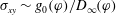 $\unicode[STIX]{x1D70E}_{xy}\sim g_{0}(\unicode[STIX]{x1D711})/D_{\infty }(\unicode[STIX]{x1D711})$
(Brady Reference Brady1993). In contrast, the above argument is not valid for non-Brownian suspensions. In fact, it is reported that
$\unicode[STIX]{x1D70E}_{xy}\sim g_{0}(\unicode[STIX]{x1D711})/D_{\infty }(\unicode[STIX]{x1D711})$
(Brady Reference Brady1993). In contrast, the above argument is not valid for non-Brownian suspensions. In fact, it is reported that
 $D_{\infty }(\unicode[STIX]{x1D711})$
increases as the density is increased and saturates at the jamming point (Leighton & Acrivos Reference Leighton and Acrivos1987a
,Reference Leighton and Acrivos
b
; Breedveld et al.
Reference Breedveld, van den Ende, Tripathi and Acrivos1998, Reference Breedveld, van den Ende, Bosscher, Jongschaap and Mellema2002; Heussinger et al.
Reference Heussinger, Berthier and Barrat2010; Olsson Reference Olsson2010). This feature can be understood from the fact that, in non-Brownian suspensions, the source of the non-affine displacement is the contact interaction between the particles, rather than the fluctuating force from the solvent. It is obvious that the contact interaction is more significant in dense suspensions, which results in larger
$D_{\infty }(\unicode[STIX]{x1D711})$
increases as the density is increased and saturates at the jamming point (Leighton & Acrivos Reference Leighton and Acrivos1987a
,Reference Leighton and Acrivos
b
; Breedveld et al.
Reference Breedveld, van den Ende, Tripathi and Acrivos1998, Reference Breedveld, van den Ende, Bosscher, Jongschaap and Mellema2002; Heussinger et al.
Reference Heussinger, Berthier and Barrat2010; Olsson Reference Olsson2010). This feature can be understood from the fact that, in non-Brownian suspensions, the source of the non-affine displacement is the contact interaction between the particles, rather than the fluctuating force from the solvent. It is obvious that the contact interaction is more significant in dense suspensions, which results in larger
 $D_{\infty }(\unicode[STIX]{x1D711})$
. This feature can be seen in the trajectory of randomly sampled particles shown in figure 5. This clearly suggests that
$D_{\infty }(\unicode[STIX]{x1D711})$
. This feature can be seen in the trajectory of randomly sampled particles shown in figure 5. This clearly suggests that
 $\unicode[STIX]{x1D70E}_{xy}\sim \unicode[STIX]{x1D6FF}\unicode[STIX]{x1D711}^{-2}$
is not the consequence of the diffusion constant in non-Brownian suspensions. Although the density dependence is similar, the underlying physics of the rheology is distinct for Brownian and non-Brownian suspensions.
$\unicode[STIX]{x1D70E}_{xy}\sim \unicode[STIX]{x1D6FF}\unicode[STIX]{x1D711}^{-2}$
is not the consequence of the diffusion constant in non-Brownian suspensions. Although the density dependence is similar, the underlying physics of the rheology is distinct for Brownian and non-Brownian suspensions.

Figure 5. Trajectory of randomly sampled particles for
 $\unicode[STIX]{x1D711}=0.30,0.60,0.635$
, from (a) to (d). The trajectory is ballistic for
$\unicode[STIX]{x1D711}=0.30,0.60,0.635$
, from (a) to (d). The trajectory is ballistic for
 $\unicode[STIX]{x1D711}=0.30$
, while it is diffusive for
$\unicode[STIX]{x1D711}=0.30$
, while it is diffusive for
 $\unicode[STIX]{x1D711}=0.635$
.
$\unicode[STIX]{x1D711}=0.635$
.
6 Validation of the postulates
In this section we articulate the crucial postulates of our theory and report the results of the simulations performed for their verification. The postulates are
(i) the factorization of the distribution function into the peculiar velocity-dependent and position-dependent parts;
(ii) Grad’s 13-moment-like expansion of the position-dependent distribution function, equation (4.7), which is an expansion around thermal equilibrium;
(iii) the factorization approximation of the multi-body correlations used in (4.20) and (4.21).
6.1 Peculiar velocity distribution function
The distribution of the peculiar velocity
 $\boldsymbol{v}_{i}=\dot{\boldsymbol{r}}_{i}-\dot{\unicode[STIX]{x1D6FE}}y_{i}\boldsymbol{e}_{x}$
is measured by MD simulation. As shown in figure 6, the peculiar velocity distribution function is nearly Gaussian in spite of the absence of any inertial effect in the dynamics. This result implies that the factorization of the distribution function assumed in (4.7) is valid. The result of our simulation supports another theoretical assumption that the base state is nearly equilibrium.
$\boldsymbol{v}_{i}=\dot{\boldsymbol{r}}_{i}-\dot{\unicode[STIX]{x1D6FE}}y_{i}\boldsymbol{e}_{x}$
is measured by MD simulation. As shown in figure 6, the peculiar velocity distribution function is nearly Gaussian in spite of the absence of any inertial effect in the dynamics. This result implies that the factorization of the distribution function assumed in (4.7) is valid. The result of our simulation supports another theoretical assumption that the base state is nearly equilibrium.

Figure 6. Distribution of the peculiar velocity measured by MD simulation (circles). The conditions are
 $\unicode[STIX]{x1D711}=0.63$
,
$\unicode[STIX]{x1D711}=0.63$
,
 $N=1000$
,
$N=1000$
,
 $\dot{\unicode[STIX]{x1D6FE}}^{\ast }=1\times 10^{-5}$
. The number of data averaged for each point is
$\dot{\unicode[STIX]{x1D6FE}}^{\ast }=1\times 10^{-5}$
. The number of data averaged for each point is
 $10^{5}$
. The figure shows the
$10^{5}$
. The figure shows the
 $x$
- and
$x$
- and
 $y$
-components. Also shown is the Gaussian distribution fitted to the measured data (solid line).
$y$
-components. Also shown is the Gaussian distribution fitted to the measured data (solid line).
6.2 Grad’s 13-moment-like expansion and factorization of multi-body correlations
We validate the expansion of the distribution of the position with the stress current, equation (4.7). For this purpose, we consider the radial distribution function at the steady state,
 $g_{\dot{\unicode[STIX]{x1D6FE}}}(\boldsymbol{r})$
, which is anisotropic under shear. It is given by
$g_{\dot{\unicode[STIX]{x1D6FE}}}(\boldsymbol{r})$
, which is anisotropic under shear. It is given by
 $$\begin{eqnarray}\displaystyle g_{\dot{\unicode[STIX]{x1D6FE}}}(\boldsymbol{r}):=\frac{1}{Nn}\left\langle \mathop{\sum }_{i}\mathop{\sum }_{j\neq i}\unicode[STIX]{x1D6FF}(\boldsymbol{r}-\boldsymbol{r}_{ij})\right\rangle =\frac{1}{Nn}\int \text{d}\unicode[STIX]{x1D71E}f(\unicode[STIX]{x1D71E})\mathop{\sum }_{i}\mathop{\sum }_{j\neq i}\unicode[STIX]{x1D6FF}(\boldsymbol{r}-\boldsymbol{r}_{ij}). & & \displaystyle\end{eqnarray}$$
From (4.7), after trivially integrating out
 $f_{eq}(\unicode[STIX]{x1D71E}_{v})$
, we obtain
$f_{eq}(\unicode[STIX]{x1D71E}_{v})$
, we obtain
 $$\begin{eqnarray}\displaystyle g_{\dot{\unicode[STIX]{x1D6FE}}}(\boldsymbol{r})=g(r)+\frac{1}{Nn}\frac{V}{2T}\unicode[STIX]{x1D6F1}_{\unicode[STIX]{x1D6FC}\unicode[STIX]{x1D6FD}}\left\langle \mathop{\sum }_{i}\mathop{\sum }_{j\neq i}\unicode[STIX]{x1D6FF}(\boldsymbol{r}-\boldsymbol{r}_{ij})\tilde{\unicode[STIX]{x1D70E}}_{\unicode[STIX]{x1D6FC}\unicode[STIX]{x1D6FD}}\right\rangle _{\!\!eq}, & & \displaystyle\end{eqnarray}$$
where
 $g(r)$
is the radial distribution function at equilibrium. By substituting the expression for the stress
$g(r)$
is the radial distribution function at equilibrium. By substituting the expression for the stress
 $\tilde{\unicode[STIX]{x1D70E}}_{\unicode[STIX]{x1D6FC}\unicode[STIX]{x1D6FD}}$
, equation (2.8) and that for the interparticle force
$\tilde{\unicode[STIX]{x1D70E}}_{\unicode[STIX]{x1D6FC}\unicode[STIX]{x1D6FD}}$
, equation (2.8) and that for the interparticle force
 $\boldsymbol{F}_{ij}^{(p)}$
therein, equation (3.8), we obtain
$\boldsymbol{F}_{ij}^{(p)}$
therein, equation (3.8), we obtain
 $$\begin{eqnarray}\displaystyle & & \displaystyle g_{\dot{\unicode[STIX]{x1D6FE}}}(\boldsymbol{r})=g(r)-\frac{1}{Nn}\frac{\unicode[STIX]{x1D701}_{e}\dot{\unicode[STIX]{x1D6FE}}d^{2}}{8T}\unicode[STIX]{x1D6F1}_{\unicode[STIX]{x1D6FC}\unicode[STIX]{x1D6FD}}\left\langle \mathop{\sum }_{i}\mathop{\sum }_{j\neq i}\mathop{\sum }_{k\neq i}\unicode[STIX]{x1D6FF}(\boldsymbol{r}-\boldsymbol{r}_{ij})r_{ik,\unicode[STIX]{x1D6FD}}\unicode[STIX]{x1D6FF}(r_{ik}-d){\mathcal{P}}(\hat{x}_{ik},{\hat{y}}_{ik})\hat{r}_{ik,\unicode[STIX]{x1D6FC}}\right\rangle _{\!\!eq}\nonumber\\ \displaystyle & & \displaystyle \quad =g(r)-\frac{1}{Nn}\frac{\unicode[STIX]{x1D701}_{e}\dot{\unicode[STIX]{x1D6FE}}d^{3}}{8T}\unicode[STIX]{x1D6F1}_{\unicode[STIX]{x1D6FC}\unicode[STIX]{x1D6FD}}\left\langle \mathop{\sum }_{i}\mathop{\sum }_{j\neq i}\mathop{\sum }_{k\neq i}\unicode[STIX]{x1D6FF}(\boldsymbol{r}-\boldsymbol{r}_{ij})\unicode[STIX]{x1D6FF}(r_{ik}-d){\mathcal{P}}(\hat{x}_{ik},{\hat{y}}_{ik})\hat{r}_{ik,\unicode[STIX]{x1D6FC}}\hat{r}_{ik,\unicode[STIX]{x1D6FD}}\right\rangle _{\!\!eq}.\nonumber\\ \displaystyle & & \displaystyle\end{eqnarray}$$
In the second equality, we have utilized
 $r_{ik,\unicode[STIX]{x1D6FD}}\unicode[STIX]{x1D6FF}(r_{ik}-d)=d\hat{r}_{ik,\unicode[STIX]{x1D6FD}}\unicode[STIX]{x1D6FF}(r_{ik}-d)$
. Equation (6.3) is expressed in terms of the triplet-correlation function
$r_{ik,\unicode[STIX]{x1D6FD}}\unicode[STIX]{x1D6FF}(r_{ik}-d)=d\hat{r}_{ik,\unicode[STIX]{x1D6FD}}\unicode[STIX]{x1D6FF}(r_{ik}-d)$
. Equation (6.3) is expressed in terms of the triplet-correlation function
 $g^{(3)}(\boldsymbol{r},\boldsymbol{r}^{\prime })$
, equation (4.19), as
$g^{(3)}(\boldsymbol{r},\boldsymbol{r}^{\prime })$
, equation (4.19), as
 $$\begin{eqnarray}\displaystyle g_{\dot{\unicode[STIX]{x1D6FE}}}(\boldsymbol{r})=g(r)-n\frac{\unicode[STIX]{x1D701}_{e}\dot{\unicode[STIX]{x1D6FE}}d^{3}}{8T}\unicode[STIX]{x1D6F1}_{\unicode[STIX]{x1D6FC}\unicode[STIX]{x1D6FD}}\int \text{d}^{3}\boldsymbol{r}^{\prime }g^{(3)}(\boldsymbol{r},\boldsymbol{r}^{\prime })\unicode[STIX]{x1D6FF}(r^{\prime }-d){\mathcal{P}}(\hat{x}^{\prime },{\hat{y}}^{\prime })\hat{r}_{\unicode[STIX]{x1D6FC}}^{\prime }\hat{r}_{\unicode[STIX]{x1D6FD}}^{\prime }. & & \displaystyle\end{eqnarray}$$
We apply the factorization approximation to
 $g^{(3)}(\boldsymbol{r},\boldsymbol{r}^{\prime })$
,
$g^{(3)}(\boldsymbol{r},\boldsymbol{r}^{\prime })$
,
 $$\begin{eqnarray}\displaystyle g^{(3)}(\boldsymbol{r},\boldsymbol{r}^{\prime })\approx g(r)g(r^{\prime })[1+h(|\boldsymbol{r}-\boldsymbol{r}^{\prime }|)], & & \displaystyle\end{eqnarray}$$
which leads to
 $$\begin{eqnarray}\displaystyle g_{\dot{\unicode[STIX]{x1D6FE}}}(\boldsymbol{r}) & {\approx} & \displaystyle g(r)\left\{1-n\frac{\unicode[STIX]{x1D701}_{e}\dot{\unicode[STIX]{x1D6FE}}d^{3}}{8T}\unicode[STIX]{x1D6F1}_{\unicode[STIX]{x1D6FC}\unicode[STIX]{x1D6FD}}\int \text{d}^{3}\boldsymbol{r}^{\prime }g(r^{\prime })[1+h(|\boldsymbol{r}-\boldsymbol{r}^{\prime }|)]\unicode[STIX]{x1D6FF}(r^{\prime }-d){\mathcal{P}}(\hat{x}^{\prime },{\hat{y}}^{\prime })\hat{r}_{\unicode[STIX]{x1D6FC}}^{\prime }\hat{r}_{\unicode[STIX]{x1D6FD}}^{\prime }\right\}\nonumber\\ \displaystyle & = & \displaystyle g(r)\left\{1-n\frac{\unicode[STIX]{x1D701}_{e}\dot{\unicode[STIX]{x1D6FE}}d^{5}}{8T}g(d)\,\unicode[STIX]{x1D6F1}_{\unicode[STIX]{x1D6FC}\unicode[STIX]{x1D6FD}}\int \text{d}{\mathcal{S}}^{\prime }[1+h(|\boldsymbol{r}-\boldsymbol{r}^{\prime }|)]{\mathcal{P}}(\hat{x}^{\prime },{\hat{y}}^{\prime })\hat{r}_{\unicode[STIX]{x1D6FC}}^{\prime }\hat{r}_{\unicode[STIX]{x1D6FD}}^{\prime }\right\}.\end{eqnarray}$$
Here,
 $h(r)=g(r)-1$
is the pair-correlation function, and
$h(r)=g(r)-1$
is the pair-correlation function, and
 $\int \text{d}{\mathcal{S}}^{\prime }\cdots \,$
denotes angular integral with respect to
$\int \text{d}{\mathcal{S}}^{\prime }\cdots \,$
denotes angular integral with respect to
 $\hat{\boldsymbol{r}}^{\prime }$
.
$\hat{\boldsymbol{r}}^{\prime }$
.

Figure 7. Definition of the angle of the separation vector.
 $\unicode[STIX]{x1D703}=135^{\circ }$
and
$\unicode[STIX]{x1D703}=135^{\circ }$
and
 $45^{\circ }$
are the compressional and extensional directions of the shear, respectively:
$45^{\circ }$
are the compressional and extensional directions of the shear, respectively:
 $\unicode[STIX]{x1D703}=0^{\circ }$
is the ‘flow direction’, which is the direction of the flow of the solvent.
$\unicode[STIX]{x1D703}=0^{\circ }$
is the ‘flow direction’, which is the direction of the flow of the solvent.
Let us consider the angular dependence of the contact value of the radial distribution function in the
 $(x,y)$
-plane. From (6.6), this is given by
$(x,y)$
-plane. From (6.6), this is given by
 $$\begin{eqnarray}\displaystyle g_{\dot{\unicode[STIX]{x1D6FE}}}(d,\unicode[STIX]{x1D703})\approx g(d)\left\{1-n\frac{\unicode[STIX]{x1D701}_{e}\dot{\unicode[STIX]{x1D6FE}}d^{5}}{8T}g(d)\,\unicode[STIX]{x1D6F1}_{\unicode[STIX]{x1D6FC}\unicode[STIX]{x1D6FD}}\int \text{d}{\mathcal{S}}^{\prime }[1+h(|\boldsymbol{r}-\boldsymbol{r}^{\prime }|)]{\mathcal{P}}(\hat{x}^{\prime },{\hat{y}}^{\prime })\hat{r}_{\unicode[STIX]{x1D6FC}}^{\prime }\hat{r}_{\unicode[STIX]{x1D6FD}}^{\prime }\right\},\qquad & & \displaystyle\end{eqnarray}$$
where
 $\unicode[STIX]{x1D703}$
is the angle of
$\unicode[STIX]{x1D703}$
is the angle of
 $\hat{\boldsymbol{r}}$
with respect to the
$\hat{\boldsymbol{r}}$
with respect to the
 $x$
-axis, and
$x$
-axis, and
 $\unicode[STIX]{x1D703}=135^{\circ }$
and
$\unicode[STIX]{x1D703}=135^{\circ }$
and
 $45^{\circ }$
are the directions of compression and extension, respectively (cf. figure 7). We adopt the approximate formula for the delta-function contribution of
$45^{\circ }$
are the directions of compression and extension, respectively (cf. figure 7). We adopt the approximate formula for the delta-function contribution of
 $h(r)$
(Donev et al.
Reference Donev, Torquato and Stillinger2005),
$h(r)$
(Donev et al.
Reference Donev, Torquato and Stillinger2005),
 $$\begin{eqnarray}\displaystyle h(r)\approx \frac{1}{4\unicode[STIX]{x1D711}\unicode[STIX]{x1D6FF}}\left[\frac{6A}{\displaystyle \left(\frac{r/d-1}{\unicode[STIX]{x1D6FF}}+C\right)^{4}}+\frac{B}{\displaystyle \left(\frac{r/d-1}{\unicode[STIX]{x1D6FF}}+C\right)^{2}}\right], & & \displaystyle\end{eqnarray}$$
where
 $\unicode[STIX]{x1D6FF}\approx (\unicode[STIX]{x1D711}_{J}-\unicode[STIX]{x1D711})/(3\unicode[STIX]{x1D711}_{J})$
and
$\unicode[STIX]{x1D6FF}\approx (\unicode[STIX]{x1D711}_{J}-\unicode[STIX]{x1D711})/(3\unicode[STIX]{x1D711}_{J})$
and
 $A=3.43,B=1.45,C=2.25$
. For the evaluation of the right-hand side of (6.7), we perform numerical integration.
$A=3.43,B=1.45,C=2.25$
. For the evaluation of the right-hand side of (6.7), we perform numerical integration.
The comparison of the both sides of (6.7) is shown in figure 8. The left-hand side is the radial distribution function at the steady state and measured by MD simulation (circles). The conditions for the simulation are described in the caption. The angular integration on the right-hand side has been evaluated as a double integral with respect to the two angles
 $(\unicode[STIX]{x1D719}_{1},\unicode[STIX]{x1D719}_{2})$
, where
$(\unicode[STIX]{x1D719}_{1},\unicode[STIX]{x1D719}_{2})$
, where
 $\cos \unicode[STIX]{x1D719}_{1}=\hat{\boldsymbol{r}}\boldsymbol{\cdot }\hat{\boldsymbol{r}}^{\prime }$
and
$\cos \unicode[STIX]{x1D719}_{1}=\hat{\boldsymbol{r}}\boldsymbol{\cdot }\hat{\boldsymbol{r}}^{\prime }$
and
 $\unicode[STIX]{x1D719}_{2}$
is the azimuthal angle of
$\unicode[STIX]{x1D719}_{2}$
is the azimuthal angle of
 $\hat{\boldsymbol{r}}^{\prime }$
around
$\hat{\boldsymbol{r}}^{\prime }$
around
 $\hat{\boldsymbol{r}}$
. These angles are bounded in the range
$\hat{\boldsymbol{r}}$
. These angles are bounded in the range
 $\unicode[STIX]{x03C0}/3<\unicode[STIX]{x1D719}_{1}<\unicode[STIX]{x03C0}$
and
$\unicode[STIX]{x03C0}/3<\unicode[STIX]{x1D719}_{1}<\unicode[STIX]{x03C0}$
and
 $0<\unicode[STIX]{x1D719}_{2}<2\unicode[STIX]{x03C0}$
, respectively. The region
$0<\unicode[STIX]{x1D719}_{2}<2\unicode[STIX]{x03C0}$
, respectively. The region
 $0<\unicode[STIX]{x1D719}_{1}<\unicode[STIX]{x03C0}/3$
is excluded to avoid overlap. The contact value of the equilibrium radial distribution function,
$0<\unicode[STIX]{x1D719}_{1}<\unicode[STIX]{x03C0}/3$
is excluded to avoid overlap. The contact value of the equilibrium radial distribution function,
 $g(d)$
, is given by
$g(d)$
, is given by
 $g_{0}(\unicode[STIX]{x1D711})\approx 0.848/(\unicode[STIX]{x1D711}_{J}-\unicode[STIX]{x1D711})$
for
$g_{0}(\unicode[STIX]{x1D711})\approx 0.848/(\unicode[STIX]{x1D711}_{J}-\unicode[STIX]{x1D711})$
for
 $\unicode[STIX]{x1D711}_{J}=0.639$
, which is approximately 100 for
$\unicode[STIX]{x1D711}_{J}=0.639$
, which is approximately 100 for
 $\unicode[STIX]{x1D711}=0.63$
. The result for the right-hand side shown in solid line in figure 8 is reduced to
$\unicode[STIX]{x1D711}=0.63$
. The result for the right-hand side shown in solid line in figure 8 is reduced to
 $1/3$
to fit the amplitude. We see that the peak in the compression direction (
$1/3$
to fit the amplitude. We see that the peak in the compression direction (
 $\unicode[STIX]{x1D703}=135^{\circ }$
) is captured by the theory, although the peak in the direction
$\unicode[STIX]{x1D703}=135^{\circ }$
) is captured by the theory, although the peak in the direction
 $\unicode[STIX]{x1D703}=0^{\circ }$
is not. The reason why the theory still reasonably predicts the stress is that the particles in contact with
$\unicode[STIX]{x1D703}=0^{\circ }$
is not. The reason why the theory still reasonably predicts the stress is that the particles in contact with
 $\unicode[STIX]{x1D703}=0^{\circ }$
does not contribute to the stress, because they are driven with the same velocity by the uniform shear.
$\unicode[STIX]{x1D703}=0^{\circ }$
does not contribute to the stress, because they are driven with the same velocity by the uniform shear.

Figure 8. Angular distribution of the contact value of the radial distribution function at the steady state measured by MD simulation (circle). The conditions are
 $\unicode[STIX]{x1D711}=0.63$
,
$\unicode[STIX]{x1D711}=0.63$
,
 $N=1000$
,
$N=1000$
,
 $\dot{\unicode[STIX]{x1D6FE}}^{\ast }=1\times 10^{-5}$
. The number of data averaged for each point is
$\dot{\unicode[STIX]{x1D6FE}}^{\ast }=1\times 10^{-5}$
. The number of data averaged for each point is
 $10^{4}$
. Also shown are the theoretical result of Grad’s expansion (solid line) and the direct measurement of Grad’s expansion (squares).
$10^{4}$
. Also shown are the theoretical result of Grad’s expansion (solid line) and the direct measurement of Grad’s expansion (squares).
For further validation, we have measured the right-hand side of (4.7) directly by MD simulation. We measure the distribution of the microscopic stress
 $\tilde{\unicode[STIX]{x1D70E}}_{\unicode[STIX]{x1D6FC}\unicode[STIX]{x1D6FD}}$
with respect to the angle of the separation vector
$\tilde{\unicode[STIX]{x1D70E}}_{\unicode[STIX]{x1D6FC}\unicode[STIX]{x1D6FD}}$
with respect to the angle of the separation vector
 $\boldsymbol{r}_{ij}$
, which resides in the
$\boldsymbol{r}_{ij}$
, which resides in the
 $(x,y)$
-plane. To extract the contribution from the contacting pairs, we have assigned 1 to
$(x,y)$
-plane. To extract the contribution from the contacting pairs, we have assigned 1 to
 $f_{eq}(\boldsymbol{r}_{ij})$
when the two particles are in contact, and 0 otherwise. The factor of
$f_{eq}(\boldsymbol{r}_{ij})$
when the two particles are in contact, and 0 otherwise. The factor of
 $(\unicode[STIX]{x03C0}/180)^{2}/Nn\times \unicode[STIX]{x0394}r\unicode[STIX]{x0394}\unicode[STIX]{x1D703}\unicode[STIX]{x0394}\unicode[STIX]{x1D719}$
is multiplied to obtain values which correspond to the radial distribution function. Here
$(\unicode[STIX]{x03C0}/180)^{2}/Nn\times \unicode[STIX]{x0394}r\unicode[STIX]{x0394}\unicode[STIX]{x1D703}\unicode[STIX]{x0394}\unicode[STIX]{x1D719}$
is multiplied to obtain values which correspond to the radial distribution function. Here
 $\unicode[STIX]{x1D719}$
is the angle of
$\unicode[STIX]{x1D719}$
is the angle of
 $\boldsymbol{r}_{ij}$
around the
$\boldsymbol{r}_{ij}$
around the
 $x$
-axis and
$x$
-axis and
 $\unicode[STIX]{x0394}r$
,
$\unicode[STIX]{x0394}r$
,
 $\unicode[STIX]{x0394}\unicode[STIX]{x1D703}$
,
$\unicode[STIX]{x0394}\unicode[STIX]{x1D703}$
,
 $\unicode[STIX]{x0394}\unicode[STIX]{x1D719}$
are the size of the bins in each direction. The result is shown in squares in figure 8. We see that the directly measured distribution has the same tendency with the theoretically evaluated distribution, i.e. both exhibit a peak in the compression direction,
$\unicode[STIX]{x0394}\unicode[STIX]{x1D719}$
are the size of the bins in each direction. The result is shown in squares in figure 8. We see that the directly measured distribution has the same tendency with the theoretically evaluated distribution, i.e. both exhibit a peak in the compression direction,
 $\unicode[STIX]{x1D703}=135^{\circ }$
, but the peak in
$\unicode[STIX]{x1D703}=135^{\circ }$
, but the peak in
 $\unicode[STIX]{x1D703}=0^{\circ }$
is not visible.
$\unicode[STIX]{x1D703}=0^{\circ }$
is not visible.
It should be noticed that the directly measured distribution does not reflect the factorization approximation, equation (6.5). Hence, this result implies the validity of (6.5). As a check for the four-body correlation, we have measured the four-point susceptibility,
 $\unicode[STIX]{x1D712}_{4}$
, by MD simulation (cf. appendix I). The result is shown in figure 9. We see that no divergence is found in
$\unicode[STIX]{x1D712}_{4}$
, by MD simulation (cf. appendix I). The result is shown in figure 9. We see that no divergence is found in
 $\unicode[STIX]{x1D712}_{4}$
near the jamming point. This implies that the divergence of the stress is determined by the divergence of the radial distribution function at contact,
$\unicode[STIX]{x1D712}_{4}$
near the jamming point. This implies that the divergence of the stress is determined by the divergence of the radial distribution function at contact,
 $g_{0}$
. Thus, our theoretical treatment based on the factorization approximation is sufficient to discuss the singularities of the stress at the jamming point.
$g_{0}$
. Thus, our theoretical treatment based on the factorization approximation is sufficient to discuss the singularities of the stress at the jamming point.

Figure 9. Four-point susceptibility measured by MD simulation. The conditions are
 $\unicode[STIX]{x1D711}=0.60-0.635$
,
$\unicode[STIX]{x1D711}=0.60-0.635$
,
 $N=1000$
,
$N=1000$
,
 $\dot{\unicode[STIX]{x1D6FE}}^{\ast }=1\times 10^{-5}$
. The number of data averaged for each point is 1000. The results are for
$\dot{\unicode[STIX]{x1D6FE}}^{\ast }=1\times 10^{-5}$
. The number of data averaged for each point is 1000. The results are for
 $\unicode[STIX]{x1D711}=0.60$
(thin solid line), 0.62 (dashed line), 0.63 (thick solid line) and 0.635 (dot-dashed line).
$\unicode[STIX]{x1D711}=0.60$
(thin solid line), 0.62 (dashed line), 0.63 (thick solid line) and 0.635 (dot-dashed line).
7 Discussion
First we discuss the hydrodynamic effects. We have formulated the theory by the resistance matrix
 $\overleftrightarrow{\unicode[STIX]{x1D701}^{(N)}}$
to include the hydrodynamic effects. In our formulation, which focuses on the proximity effects of the particles, the far-field part of
$\overleftrightarrow{\unicode[STIX]{x1D701}^{(N)}}$
to include the hydrodynamic effects. In our formulation, which focuses on the proximity effects of the particles, the far-field part of
 $\overleftrightarrow{\unicode[STIX]{x1D701}^{(N)}}$
drops out, and the lubrication part
$\overleftrightarrow{\unicode[STIX]{x1D701}^{(N)}}$
drops out, and the lubrication part
 $\overleftrightarrow{\unicode[STIX]{x1D701}_{lub}^{(2)}}$
is taken into account. Although we have compared the theory and the MD simulation for the simplified case where
$\overleftrightarrow{\unicode[STIX]{x1D701}_{lub}^{(2)}}$
is taken into account. Although we have compared the theory and the MD simulation for the simplified case where
 $\overleftrightarrow{\unicode[STIX]{x1D701}_{lub}^{(2)}}$
is proportional to the unit tensor, it is possible to do so for a more generic case. This is left for future work.
$\overleftrightarrow{\unicode[STIX]{x1D701}_{lub}^{(2)}}$
is proportional to the unit tensor, it is possible to do so for a more generic case. This is left for future work.
Next we discuss the effect of the contact force of the particles. In this work we have considered frictionless spheres, but it is reported that the exponent of the divergence
 $\unicode[STIX]{x1D706}$
depends on the friction between the particles;
$\unicode[STIX]{x1D706}$
depends on the friction between the particles;
 $\unicode[STIX]{x1D706}=1.6$
for frictionless spheres, while
$\unicode[STIX]{x1D706}=1.6$
for frictionless spheres, while
 $\unicode[STIX]{x1D706}=2.4$
in the strong friction limit (Mari et al.
Reference Mari, Seto, Morris and Denn2014). Note that the jamming density
$\unicode[STIX]{x1D706}=2.4$
in the strong friction limit (Mari et al.
Reference Mari, Seto, Morris and Denn2014). Note that the jamming density
 $\unicode[STIX]{x1D711}_{J}$
used in Mari et al. (Reference Mari, Seto, Morris and Denn2014) is 0.66, which reduces the exponent. Extension of this work to frictional particles is necessary to address this issue (Saitoh & Hayakawa Reference Saitoh and Hayakawa2019).
$\unicode[STIX]{x1D711}_{J}$
used in Mari et al. (Reference Mari, Seto, Morris and Denn2014) is 0.66, which reduces the exponent. Extension of this work to frictional particles is necessary to address this issue (Saitoh & Hayakawa Reference Saitoh and Hayakawa2019).
In the course of the derivation, we have assumed a separation between
 $O(g_{0}(\unicode[STIX]{x1D711}))^{2}$
and
$O(g_{0}(\unicode[STIX]{x1D711}))^{2}$
and
 $O(g_{0}(\unicode[STIX]{x1D711}))$
terms as in (4.30) and (4.31). This assumption is valid when the magnitudes of
$O(g_{0}(\unicode[STIX]{x1D711}))$
terms as in (4.30) and (4.31). This assumption is valid when the magnitudes of
 $O(g_{0}(\unicode[STIX]{x1D711}))^{2}$
and
$O(g_{0}(\unicode[STIX]{x1D711}))^{2}$
and
 $O(g_{0}(\unicode[STIX]{x1D711}))$
terms are well separated, which holds for larger
$O(g_{0}(\unicode[STIX]{x1D711}))$
terms are well separated, which holds for larger
 $\unicode[STIX]{x1D6EC}$
or
$\unicode[STIX]{x1D6EC}$
or
 $\unicode[STIX]{x1D711}$
closer to
$\unicode[STIX]{x1D711}$
closer to
 $\unicode[STIX]{x1D711}_{J}$
(
$\unicode[STIX]{x1D711}_{J}$
(
 $\unicode[STIX]{x1D6FF}\unicode[STIX]{x1D711}$
closer to zero). For the case
$\unicode[STIX]{x1D6FF}\unicode[STIX]{x1D711}$
closer to zero). For the case
 $\unicode[STIX]{x1D6EC}=0.04$
, this separation is reasonable only for
$\unicode[STIX]{x1D6EC}=0.04$
, this separation is reasonable only for
 $\unicode[STIX]{x1D6FF}\unicode[STIX]{x1D711}<0.001$
, so the applicability below the jamming point must be perceived restricted than presented, as shown in § D.2.
$\unicode[STIX]{x1D6FF}\unicode[STIX]{x1D711}<0.001$
, so the applicability below the jamming point must be perceived restricted than presented, as shown in § D.2.
Finally, we compare our theory with DeGiuli et al. (Reference DeGiuli, Düring, Lerner and Wyart2015), which derives constitutive laws
 $\unicode[STIX]{x1D6FF}\unicode[STIX]{x1D711}(J)\sim J^{b_{\unicode[STIX]{x1D711}}}$
i.e.
$\unicode[STIX]{x1D6FF}\unicode[STIX]{x1D711}(J)\sim J^{b_{\unicode[STIX]{x1D711}}}$
i.e.
 $\unicode[STIX]{x1D702}_{n}\sim \unicode[STIX]{x1D6FF}\unicode[STIX]{x1D711}^{-1/b_{\unicode[STIX]{x1D711}}}$
and
$\unicode[STIX]{x1D702}_{n}\sim \unicode[STIX]{x1D6FF}\unicode[STIX]{x1D711}^{-1/b_{\unicode[STIX]{x1D711}}}$
and
 $\unicode[STIX]{x1D707}(J)-\unicode[STIX]{x1D707}_{0}\sim J^{b_{\unicode[STIX]{x1D707}}}$
with
$\unicode[STIX]{x1D707}(J)-\unicode[STIX]{x1D707}_{0}\sim J^{b_{\unicode[STIX]{x1D707}}}$
with
 $b_{\unicode[STIX]{x1D711}}=b_{\unicode[STIX]{x1D707}}\approx 0.35$
, under the assumption that
$b_{\unicode[STIX]{x1D711}}=b_{\unicode[STIX]{x1D707}}\approx 0.35$
, under the assumption that
 $\unicode[STIX]{x1D702}_{s}$
and
$\unicode[STIX]{x1D702}_{s}$
and
 $\unicode[STIX]{x1D702}_{n}$
diverges identically. The equality
$\unicode[STIX]{x1D702}_{n}$
diverges identically. The equality
 $b_{\unicode[STIX]{x1D711}}=b_{\unicode[STIX]{x1D707}}$
suggests
$b_{\unicode[STIX]{x1D711}}=b_{\unicode[STIX]{x1D707}}$
suggests
 $\unicode[STIX]{x1D6FF}\unicode[STIX]{x1D711}\sim \unicode[STIX]{x1D6FF}\unicode[STIX]{x1D707}$
, which is consistent with our theory, equation (4.45), but the exponent of the divergence
$\unicode[STIX]{x1D6FF}\unicode[STIX]{x1D711}\sim \unicode[STIX]{x1D6FF}\unicode[STIX]{x1D707}$
, which is consistent with our theory, equation (4.45), but the exponent of the divergence
 $1/b_{\unicode[STIX]{x1D711}}\approx 2.83$
differs from our prediction of 2. Their exponent relies on
$1/b_{\unicode[STIX]{x1D711}}\approx 2.83$
differs from our prediction of 2. Their exponent relies on
 $g^{\prime }(r)$
for
$g^{\prime }(r)$
for
 $r>d$
, so it might be applicable to soft-core systems (Kawasaki et al.
Reference Kawasaki, Coslovich, Ikeda and Berthier2015). However, this is incompatible with hard spheres, because of (3.15). Note that their model does not consider the hydrodynamic interactions.
$r>d$
, so it might be applicable to soft-core systems (Kawasaki et al.
Reference Kawasaki, Coslovich, Ikeda and Berthier2015). However, this is incompatible with hard spheres, because of (3.15). Note that their model does not consider the hydrodynamic interactions.
8 Concluding remarks
In this paper, we have derived approximate analytic formulas for the shear viscosity
 $\unicode[STIX]{x1D702}_{s}$
, pressure viscosity
$\unicode[STIX]{x1D702}_{s}$
, pressure viscosity
 $\unicode[STIX]{x1D702}_{n}$
and the stress ratio
$\unicode[STIX]{x1D702}_{n}$
and the stress ratio
 $\unicode[STIX]{x1D707}$
for dense non-Brownian suspensions, valid at
$\unicode[STIX]{x1D707}$
for dense non-Brownian suspensions, valid at
 $\unicode[STIX]{x1D711}\lesssim \unicode[STIX]{x1D711}_{J}$
. These formulas are derived from the microscopic overdamped equation of motion for suspended frictionless hard spheres, taking into account the proximity lubrication effect of the hydrodynamic interactions, and the approximate distribution function which is an extension of Grad’s 13-moment-like expansion. We have performed MD simulations and confirmed that our theory successfully derives the relations
$\unicode[STIX]{x1D711}\lesssim \unicode[STIX]{x1D711}_{J}$
. These formulas are derived from the microscopic overdamped equation of motion for suspended frictionless hard spheres, taking into account the proximity lubrication effect of the hydrodynamic interactions, and the approximate distribution function which is an extension of Grad’s 13-moment-like expansion. We have performed MD simulations and confirmed that our theory successfully derives the relations
 $\unicode[STIX]{x1D702}_{s}/\unicode[STIX]{x1D702}_{0}\sim \unicode[STIX]{x1D702}_{n}/\unicode[STIX]{x1D702}_{0}\sim \unicode[STIX]{x1D6FF}\unicode[STIX]{x1D711}^{-2}$
and
$\unicode[STIX]{x1D702}_{s}/\unicode[STIX]{x1D702}_{0}\sim \unicode[STIX]{x1D702}_{n}/\unicode[STIX]{x1D702}_{0}\sim \unicode[STIX]{x1D6FF}\unicode[STIX]{x1D711}^{-2}$
and
 $\unicode[STIX]{x1D707}-\unicode[STIX]{x1D707}_{0}\sim \unicode[STIX]{x1D6FF}\unicode[STIX]{x1D711}$
, where
$\unicode[STIX]{x1D707}-\unicode[STIX]{x1D707}_{0}\sim \unicode[STIX]{x1D6FF}\unicode[STIX]{x1D711}$
, where
 $\unicode[STIX]{x1D6FF}\unicode[STIX]{x1D711}=\unicode[STIX]{x1D711}_{J}-\unicode[STIX]{x1D711}$
and
$\unicode[STIX]{x1D6FF}\unicode[STIX]{x1D711}=\unicode[STIX]{x1D711}_{J}-\unicode[STIX]{x1D711}$
and
 $\unicode[STIX]{x1D707}_{0}\approx 0.16$
.
$\unicode[STIX]{x1D707}_{0}\approx 0.16$
.
Acknowledgements
The authors are grateful to S. Takada for providing the prototype of the program for the event-driven MD simulation. They are also grateful to K. Saitoh, A. Ikeda, T. Kawasaki, Y. Oono, R. Mari and R. Seto for fruitful discussions on the subject. One of the authors (H.H.) appreciates useful comments by P. R. Nott and C. O’Hern. This work is partially supported by the Grant-in-Aid of MEXT for Scientific Research (grants no. 16H04025). The MD simulations for this work have been carried out at the computer facilities at the Yukawa Institute of Theoretical Physics, Kyoto University.
Appendix A. Force correlations
We derive explicit expressions for the second term on the right-hand side of (2.9), which includes a derivative of the interparticle forces. Note that collisions take place only when the interparticle distance is equal to the diameter in assemblies of hard spheres. Hence, the derivative acts only on the angular coordinates, e.g.
 $$\begin{eqnarray}\displaystyle \frac{\unicode[STIX]{x2202}F_{j,\unicode[STIX]{x1D6FC}}^{(p)}}{\unicode[STIX]{x2202}r_{i,\unicode[STIX]{x1D706}}} & = & \displaystyle \frac{1}{2}\unicode[STIX]{x1D701}\dot{\unicode[STIX]{x1D6FE}}d^{2}\mathop{\sum }_{k\neq j}\unicode[STIX]{x1D6FF}(r_{jk}-d)\frac{\unicode[STIX]{x2202}}{\unicode[STIX]{x2202}r_{i,\unicode[STIX]{x1D706}}}[{\mathcal{P}}(\hat{x}_{jk},{\hat{y}}_{jk})\hat{r}_{jk,\unicode[STIX]{x1D6FC}}]\nonumber\\ \displaystyle & = & \displaystyle \frac{1}{2}\unicode[STIX]{x1D701}\dot{\unicode[STIX]{x1D6FE}}d^{2}\mathop{\sum }_{k\neq j}\unicode[STIX]{x1D6FF}(r_{jk}-d)\unicode[STIX]{x1D6E9}(-\hat{x}_{jk}{\hat{y}}_{jk})\frac{\unicode[STIX]{x2202}}{\unicode[STIX]{x2202}r_{i,\unicode[STIX]{x1D706}}}[-\hat{x}_{jk}{\hat{y}}_{jk}\hat{r}_{jk,\unicode[STIX]{x1D6FC}}].\end{eqnarray}$$
Here, the derivative of
 $\unicode[STIX]{x1D6E9}(-\hat{x}{\hat{y}})=\unicode[STIX]{x1D6E9}(\hat{x})\unicode[STIX]{x1D6E9}(-{\hat{y}})+\unicode[STIX]{x1D6E9}(-\hat{x})\unicode[STIX]{x1D6E9}({\hat{y}})$
vanishes since it yields
$\unicode[STIX]{x1D6E9}(-\hat{x}{\hat{y}})=\unicode[STIX]{x1D6E9}(\hat{x})\unicode[STIX]{x1D6E9}(-{\hat{y}})+\unicode[STIX]{x1D6E9}(-\hat{x})\unicode[STIX]{x1D6E9}({\hat{y}})$
vanishes since it yields
 $\hat{x}\unicode[STIX]{x1D6FF}(\hat{x})$
or
$\hat{x}\unicode[STIX]{x1D6FF}(\hat{x})$
or
 ${\hat{y}}\unicode[STIX]{x1D6FF}({\hat{y}})$
. This is explicitly confirmed by
${\hat{y}}\unicode[STIX]{x1D6FF}({\hat{y}})$
. This is explicitly confirmed by
 $$\begin{eqnarray}\displaystyle \hat{x}{\hat{y}}\hat{r}_{\unicode[STIX]{x1D6FC}}\frac{\unicode[STIX]{x2202}}{\unicode[STIX]{x2202}\hat{r}_{\unicode[STIX]{x1D706}}}\unicode[STIX]{x1D6E9}(-\hat{x}{\hat{y}})=\hat{x}{\hat{y}}\hat{r}_{\unicode[STIX]{x1D6FC}}[\unicode[STIX]{x1D6FF}_{\unicode[STIX]{x1D706}x}\unicode[STIX]{x1D6FF}(\hat{x})\unicode[STIX]{x1D6E9}(-{\hat{y}})-\unicode[STIX]{x1D6FF}_{\unicode[STIX]{x1D706}y}\unicode[STIX]{x1D6E9}(\hat{x})\unicode[STIX]{x1D6FF}({\hat{y}})-\unicode[STIX]{x1D6FF}_{\unicode[STIX]{x1D706}x}\unicode[STIX]{x1D6FF}(\hat{x})\unicode[STIX]{x1D6E9}({\hat{y}})+\unicode[STIX]{x1D6FF}_{\unicode[STIX]{x1D706}y}\unicode[STIX]{x1D6E9}(\hat{x})\unicode[STIX]{x1D6FF}({\hat{y}})], & & \displaystyle \nonumber\\ \displaystyle & & \displaystyle\end{eqnarray}$$
where each term includes
 $\hat{x}\unicode[STIX]{x1D6FF}(\hat{x})$
or
$\hat{x}\unicode[STIX]{x1D6FF}(\hat{x})$
or
 ${\hat{y}}\unicode[STIX]{x1D6FF}({\hat{y}})$
. From (A 1), the third term on the right-hand side of (2.9) is evaluated as
${\hat{y}}\unicode[STIX]{x1D6FF}({\hat{y}})$
. From (A 1), the third term on the right-hand side of (2.9) is evaluated as
 $$\begin{eqnarray}\displaystyle & & \displaystyle \mathop{\sum }_{i,j}\left\langle F_{i,\unicode[STIX]{x1D706}}^{(p)}r_{j,\unicode[STIX]{x1D6FD}}\frac{\unicode[STIX]{x2202}F_{j,\unicode[STIX]{x1D6FC}}^{(p)}}{\unicode[STIX]{x2202}r_{i,\unicode[STIX]{x1D706}}}\right\rangle \nonumber\\ \displaystyle & & \displaystyle \quad =\frac{1}{2}\unicode[STIX]{x1D701}\mathop{\sum }_{i,j}\left\langle F_{i,\unicode[STIX]{x1D706}}^{(p)}r_{j,\unicode[STIX]{x1D6FD}}\dot{\unicode[STIX]{x1D6FE}}d^{2}\mathop{\sum }_{k\neq j}\unicode[STIX]{x1D6FF}(r_{jk}-d)\unicode[STIX]{x1D6E9}(-\hat{x}_{jk}{\hat{y}}_{jk})\frac{\unicode[STIX]{x2202}}{\unicode[STIX]{x2202}r_{i,\unicode[STIX]{x1D706}}}[-\hat{x}_{jk}{\hat{y}}_{jk}\hat{r}_{jk,\unicode[STIX]{x1D6FC}}]\right\rangle \nonumber\\ \displaystyle & & \displaystyle \quad =-\frac{1}{2}\unicode[STIX]{x1D701}\mathop{\sum }_{i,j}\left\langle F_{i,\unicode[STIX]{x1D706}}^{(p)}r_{j,\unicode[STIX]{x1D6FD}}\dot{\unicode[STIX]{x1D6FE}}d\mathop{\sum }_{k\neq j}\tilde{\unicode[STIX]{x1D6E5}}_{jk}\unicode[STIX]{x1D6E9}_{jk}(\unicode[STIX]{x1D6FF}_{ij}-\unicode[STIX]{x1D6FF}_{ik})(\unicode[STIX]{x1D6FF}_{\unicode[STIX]{x1D706}x}{\hat{y}}_{jk}\hat{r}_{jk,\unicode[STIX]{x1D6FC}}+\unicode[STIX]{x1D6FF}_{\unicode[STIX]{x1D706}y}\hat{x}_{jk}\hat{r}_{jk,\unicode[STIX]{x1D6FC}}+\unicode[STIX]{x1D6FF}_{\unicode[STIX]{x1D706}\unicode[STIX]{x1D6FC}}\hat{x}_{jk}{\hat{y}}_{jk})\right\rangle \nonumber\\ \displaystyle & & \displaystyle \quad =-\frac{1}{2}\unicode[STIX]{x1D701}\dot{\unicode[STIX]{x1D6FE}}d^{2}\mathop{\sum }_{i}\mathop{\sum }_{j\neq i}\langle F_{i,\unicode[STIX]{x1D706}}^{(p)}\hat{r}_{ij,\unicode[STIX]{x1D6FD}}\tilde{\unicode[STIX]{x1D6E5}}_{ij}\unicode[STIX]{x1D6E9}_{ij}(\unicode[STIX]{x1D6FF}_{\unicode[STIX]{x1D706}x}{\hat{y}}_{ij}\hat{r}_{ij,\unicode[STIX]{x1D6FC}}+\unicode[STIX]{x1D6FF}_{\unicode[STIX]{x1D706}y}\hat{x}_{ij}\hat{r}_{ij,\unicode[STIX]{x1D6FC}}+\unicode[STIX]{x1D6FF}_{\unicode[STIX]{x1D706}\unicode[STIX]{x1D6FC}}\hat{x}_{ij}{\hat{y}}_{ij})\rangle \nonumber\\ \displaystyle & & \displaystyle \quad =-\frac{1}{2}\unicode[STIX]{x1D701}\dot{\unicode[STIX]{x1D6FE}}d^{2}\mathop{\sum }_{i}\mathop{\sum }_{j\neq i}\langle F_{i,\unicode[STIX]{x1D706}}^{(p)}\hat{r}_{ij,\unicode[STIX]{x1D6FD}}(\unicode[STIX]{x1D6FF}_{\unicode[STIX]{x1D706}x}\unicode[STIX]{x1D6E5}_{ij}^{\unicode[STIX]{x1D6FC}y}+\unicode[STIX]{x1D6FF}_{\unicode[STIX]{x1D706}y}\unicode[STIX]{x1D6E5}_{ij}^{\unicode[STIX]{x1D6FC}x}+\unicode[STIX]{x1D6FF}_{\unicode[STIX]{x1D706}\unicode[STIX]{x1D6FC}}\unicode[STIX]{x1D6E5}_{ij}^{xy})\rangle ,\end{eqnarray}$$
where
 $r_{j,\unicode[STIX]{x1D6FD}}$
is cast into a relative coordinate
$r_{j,\unicode[STIX]{x1D6FD}}$
is cast into a relative coordinate
 $r_{ij,\unicode[STIX]{x1D6FD}}$
in the third equality, and
$r_{ij,\unicode[STIX]{x1D6FD}}$
in the third equality, and
 $\tilde{\unicode[STIX]{x1D6E5}}_{ij}:=\unicode[STIX]{x1D6FF}(r_{ij}-d)$
,
$\tilde{\unicode[STIX]{x1D6E5}}_{ij}:=\unicode[STIX]{x1D6FF}(r_{ij}-d)$
,
 $\unicode[STIX]{x1D6E9}_{ij}:=\unicode[STIX]{x1D6E9}(-\hat{x}_{ij}{\hat{y}}_{ij})$
,
$\unicode[STIX]{x1D6E9}_{ij}:=\unicode[STIX]{x1D6E9}(-\hat{x}_{ij}{\hat{y}}_{ij})$
,
 $\unicode[STIX]{x1D6E5}_{ij}^{\unicode[STIX]{x1D6FC}\unicode[STIX]{x1D6FD}}:=\tilde{\unicode[STIX]{x1D6E5}}_{ij}\hat{r}_{ij,\unicode[STIX]{x1D6FC}}\hat{r}_{ij,\unicode[STIX]{x1D6FD}}\unicode[STIX]{x1D6E9}_{ij}$
(cf. (4.2)). Note that relative coordinates, e.g.
$\unicode[STIX]{x1D6E5}_{ij}^{\unicode[STIX]{x1D6FC}\unicode[STIX]{x1D6FD}}:=\tilde{\unicode[STIX]{x1D6E5}}_{ij}\hat{r}_{ij,\unicode[STIX]{x1D6FC}}\hat{r}_{ij,\unicode[STIX]{x1D6FD}}\unicode[STIX]{x1D6E9}_{ij}$
(cf. (4.2)). Note that relative coordinates, e.g.
 $r_{ij,\unicode[STIX]{x1D6FD}}$
, are expressed in terms of normalized relative coordinates
$r_{ij,\unicode[STIX]{x1D6FD}}$
, are expressed in terms of normalized relative coordinates
 $\hat{r}_{ij,\unicode[STIX]{x1D6FD}}$
as
$\hat{r}_{ij,\unicode[STIX]{x1D6FD}}$
as
 $r_{ij}=d\hat{r}_{ij,\unicode[STIX]{x1D6FD}}$
, due to the delta function
$r_{ij}=d\hat{r}_{ij,\unicode[STIX]{x1D6FD}}$
, due to the delta function
 $\unicode[STIX]{x1D6FF}(r_{ij}-d)$
. If we further substitute
$\unicode[STIX]{x1D6FF}(r_{ij}-d)$
. If we further substitute
 $F_{i,\unicode[STIX]{x1D706}}^{(p)}=\sum _{j\neq i}F_{ij,\unicode[STIX]{x1D706}}^{(p)}$
, where
$F_{i,\unicode[STIX]{x1D706}}^{(p)}=\sum _{j\neq i}F_{ij,\unicode[STIX]{x1D706}}^{(p)}$
, where
 $F_{ij,\unicode[STIX]{x1D706}}^{(p)}$
is given by (3.15), we obtain
$F_{ij,\unicode[STIX]{x1D706}}^{(p)}$
is given by (3.15), we obtain
 $$\begin{eqnarray}\displaystyle & & \displaystyle \mathop{\sum }_{i,j}\left\langle F_{i,\unicode[STIX]{x1D706}}^{(p)}r_{j,\unicode[STIX]{x1D6FD}}\frac{\unicode[STIX]{x2202}F_{j,\unicode[STIX]{x1D6FC}}^{(p)}}{\unicode[STIX]{x2202}r_{i,\unicode[STIX]{x1D706}}}\right\rangle \nonumber\\ \displaystyle & & \displaystyle \quad =\frac{1}{4}\unicode[STIX]{x1D701}^{2}\dot{\unicode[STIX]{x1D6FE}}^{2}d^{4}\mathop{\sum }_{i}\mathop{\sum }_{j\neq i}\mathop{\sum }_{k\neq i}\langle \tilde{\unicode[STIX]{x1D6E5}}_{ik}\hat{r}_{ik,\unicode[STIX]{x1D706}}\hat{x}_{ik}{\hat{y}}_{ik}\unicode[STIX]{x1D6E9}_{ik}\hat{r}_{ij,\unicode[STIX]{x1D6FD}}(\unicode[STIX]{x1D6FF}_{\unicode[STIX]{x1D706}x}\unicode[STIX]{x1D6E5}_{ij}^{\unicode[STIX]{x1D6FC}y}+\unicode[STIX]{x1D6FF}_{\unicode[STIX]{x1D706}y}\unicode[STIX]{x1D6E5}_{ij}^{\unicode[STIX]{x1D6FC}x}+\unicode[STIX]{x1D6FF}_{\unicode[STIX]{x1D706}\unicode[STIX]{x1D6FC}}\unicode[STIX]{x1D6E5}_{ij}^{xy})\rangle \nonumber\\ \displaystyle & & \displaystyle \quad =\frac{1}{4}\unicode[STIX]{x1D701}^{2}\dot{\unicode[STIX]{x1D6FE}}^{2}d^{4}\mathop{\sum }_{i}\mathop{\sum }_{j\neq i}\mathop{\sum }_{k\neq i}\langle \unicode[STIX]{x1D6E5}_{ik}^{xy}\hat{r}_{ik,\unicode[STIX]{x1D706}}\hat{r}_{ij,\unicode[STIX]{x1D6FD}}(\unicode[STIX]{x1D6FF}_{\unicode[STIX]{x1D706}x}\unicode[STIX]{x1D6E5}_{ij}^{\unicode[STIX]{x1D6FC}y}+\unicode[STIX]{x1D6FF}_{\unicode[STIX]{x1D706}y}\unicode[STIX]{x1D6E5}_{ij}^{\unicode[STIX]{x1D6FC}x}+\unicode[STIX]{x1D6FF}_{\unicode[STIX]{x1D706}\unicode[STIX]{x1D6FC}}\unicode[STIX]{x1D6E5}_{ij}^{xy})\rangle \nonumber\\ \displaystyle & & \displaystyle \quad =\frac{1}{4}\unicode[STIX]{x1D701}^{2}\dot{\unicode[STIX]{x1D6FE}}^{2}d^{4}\mathop{\sum }_{i}\mathop{\sum }_{j\neq i}\mathop{\sum }_{k\neq i}\langle \unicode[STIX]{x1D6E5}_{ik}^{xy}\hat{r}_{ij,\unicode[STIX]{x1D6FD}}(\hat{x}_{ik}\unicode[STIX]{x1D6E5}_{ij}^{\unicode[STIX]{x1D6FC}y}+{\hat{y}}_{ik}\unicode[STIX]{x1D6E5}_{ij}^{\unicode[STIX]{x1D6FC}x}+\hat{r}_{ik,\unicode[STIX]{x1D6FC}}\unicode[STIX]{x1D6E5}_{ij}^{xy})\rangle .\end{eqnarray}$$
This can further be cast in the form
 $$\begin{eqnarray}\displaystyle & & \displaystyle \mathop{\sum }_{i,j}\left\langle F_{i,\unicode[STIX]{x1D706}}^{(p)}r_{j,\unicode[STIX]{x1D6FD}}\frac{\unicode[STIX]{x2202}F_{j,\unicode[STIX]{x1D6FC}}^{(p)}}{\unicode[STIX]{x2202}r_{i,\unicode[STIX]{x1D706}}}\right\rangle \nonumber\\ \displaystyle & & \displaystyle \quad =\frac{1}{4}\unicode[STIX]{x1D701}^{2}\dot{\unicode[STIX]{x1D6FE}}^{2}d^{4}\mathop{\sum }_{i}\mathop{\sum }_{j\neq i}\mathop{\sum }_{k\neq i}\langle \unicode[STIX]{x1D6E5}_{ij}^{xy}\unicode[STIX]{x1D6E5}_{ik}^{xy}\hat{r}_{ij,\unicode[STIX]{x1D6FD}}\hat{r}_{ik,\unicode[STIX]{x1D6FC}}+\unicode[STIX]{x1D6E5}_{ij}^{\unicode[STIX]{x1D6FC}\unicode[STIX]{x1D6FD}}\unicode[STIX]{x1D6E5}_{ik}^{xy}(\hat{x}_{ij}{\hat{y}}_{ik}+{\hat{y}}_{ij}\hat{x}_{ik})\rangle\end{eqnarray}$$
by the identities
 $\hat{r}_{ij,\unicode[STIX]{x1D6FD}}\unicode[STIX]{x1D6E5}_{ij}^{\unicode[STIX]{x1D6FC}y}={\hat{y}}_{ij}\unicode[STIX]{x1D6E5}_{ij}^{\unicode[STIX]{x1D6FC}\unicode[STIX]{x1D6FD}}$
and
$\hat{r}_{ij,\unicode[STIX]{x1D6FD}}\unicode[STIX]{x1D6E5}_{ij}^{\unicode[STIX]{x1D6FC}y}={\hat{y}}_{ij}\unicode[STIX]{x1D6E5}_{ij}^{\unicode[STIX]{x1D6FC}\unicode[STIX]{x1D6FD}}$
and
 $\hat{r}_{ij,\unicode[STIX]{x1D6FD}}\unicode[STIX]{x1D6E5}_{ij}^{\unicode[STIX]{x1D6FC}x}=\hat{x}_{ij}\unicode[STIX]{x1D6E5}_{ij}^{\unicode[STIX]{x1D6FC}\unicode[STIX]{x1D6FD}}$
.
$\hat{r}_{ij,\unicode[STIX]{x1D6FD}}\unicode[STIX]{x1D6E5}_{ij}^{\unicode[STIX]{x1D6FC}x}=\hat{x}_{ij}\unicode[STIX]{x1D6E5}_{ij}^{\unicode[STIX]{x1D6FC}\unicode[STIX]{x1D6FD}}$
.
Appendix B. Approximation of the force correlations
First we derive approximate expressions for the force correlations which appear on the right-hand side of (4.5), by means of the approximate formula (4.9). Then we apply the factorization approximation to the multi-body correlations to obtain the final approximate expressions.
B.1 Application of Grad’s 13-moment-like expansion
B.1.1 Canonical terms
Let us consider the first term on the right-hand side of (4.5) for illustration. The second term can be evaluated in parallel. The corresponding canonical term, i.e. the first term on the right-hand side of (4.9), includes three indices
 $i,j,k$
for the particles. This can be decomposed into three- and two-body correlations as follows,
$i,j,k$
for the particles. This can be decomposed into three- and two-body correlations as follows,
 $$\begin{eqnarray}\displaystyle & & \displaystyle \mathop{\sum }_{i=1}^{N}\mathop{\sum }_{j\neq i}\mathop{\sum }_{k\neq i}\langle \unicode[STIX]{x1D6E5}_{ij}^{xy}\unicode[STIX]{x1D6E5}_{ik}^{xy}(\hat{r}_{ij,\unicode[STIX]{x1D6FC}}\hat{r}_{ik,\unicode[STIX]{x1D6FD}}+\hat{r}_{ij,\unicode[STIX]{x1D6FD}}\hat{r}_{ik,\unicode[STIX]{x1D6FC}})\rangle _{eq}\nonumber\\ \displaystyle & & \displaystyle \quad =\sum _{i,j,k}\langle \unicode[STIX]{x1D6E5}_{ij}^{xy}\unicode[STIX]{x1D6E5}_{ik}^{xy}(\hat{r}_{ij,\unicode[STIX]{x1D6FC}}\hat{r}_{ik,\unicode[STIX]{x1D6FD}}+\hat{r}_{ij,\unicode[STIX]{x1D6FD}}\hat{r}_{ik,\unicode[STIX]{x1D6FC}})\rangle _{eq}+\frac{2}{d}\sum _{i,j}\langle \tilde{\unicode[STIX]{x1D6E5}}_{ij}\hat{r}_{ij,\unicode[STIX]{x1D6FC}}\hat{r}_{ij,\unicode[STIX]{x1D6FD}}\hat{x}_{ij}^{2}{\hat{y}}_{ij}^{2}\unicode[STIX]{x1D6E9}_{ij}\rangle _{eq},\end{eqnarray}$$
where
 $\tilde{\unicode[STIX]{x1D6E5}}_{ij}:=\unicode[STIX]{x1D6FF}(r_{ij}-d)$
,
$\tilde{\unicode[STIX]{x1D6E5}}_{ij}:=\unicode[STIX]{x1D6FF}(r_{ij}-d)$
,
 $\unicode[STIX]{x1D6E9}_{ij}:=\unicode[STIX]{x1D6E9}(-\hat{x}_{ij}{\hat{y}}_{ij})$
and
$\unicode[STIX]{x1D6E9}_{ij}:=\unicode[STIX]{x1D6E9}(-\hat{x}_{ij}{\hat{y}}_{ij})$
and
 $\unicode[STIX]{x1D6E5}_{ij}^{\unicode[STIX]{x1D6FC}\unicode[STIX]{x1D6FD}}$
is given by (4.2). Here, the summation
$\unicode[STIX]{x1D6E5}_{ij}^{\unicode[STIX]{x1D6FC}\unicode[STIX]{x1D6FD}}$
is given by (4.2). Here, the summation
 $\sum _{i,j,k}^{\prime \prime }$
is performed over (
$\sum _{i,j,k}^{\prime \prime }$
is performed over (
 $i,j,k$
) where all the indices are different, i.e.
$i,j,k$
) where all the indices are different, i.e.
 $i\neq j$
,
$i\neq j$
,
 $j\neq k$
and
$j\neq k$
and
 $k\neq i$
, and the summation
$k\neq i$
, and the summation
 $\sum _{i,j}^{\prime }$
is done for
$\sum _{i,j}^{\prime }$
is done for
 $i\neq j$
. The two-body correlation term (second term) is obtained by setting
$i\neq j$
. The two-body correlation term (second term) is obtained by setting
 $j=k$
in the three-body correlation term (first term). Equation (B 1) can be further expressed as
$j=k$
in the three-body correlation term (first term). Equation (B 1) can be further expressed as
 $$\begin{eqnarray}\displaystyle & & \displaystyle \mathop{\sum }_{i=1}^{N}\mathop{\sum }_{j\neq i}\mathop{\sum }_{k\neq i}\langle \unicode[STIX]{x1D6E5}_{ij}^{xy}\unicode[STIX]{x1D6E5}_{ik}^{xy}(\hat{r}_{ij,\unicode[STIX]{x1D6FC}}\hat{r}_{ik,\unicode[STIX]{x1D6FD}}+\hat{r}_{ij,\unicode[STIX]{x1D6FD}}\hat{r}_{ik,\unicode[STIX]{x1D6FC}})\rangle _{eq}\nonumber\\ \displaystyle & & \displaystyle \quad =Nn(\unicode[STIX]{x1D711})^{2}\int \text{d}^{3}\boldsymbol{r}\int \text{d}^{3}\boldsymbol{r}^{\prime }g^{(3)}(\boldsymbol{r},\boldsymbol{r}^{\prime })\unicode[STIX]{x1D6FF}(r-d)\unicode[STIX]{x1D6FF}(r^{\prime }-d)(\hat{r}_{\unicode[STIX]{x1D6FC}}\hat{r}_{\unicode[STIX]{x1D6FD}}^{\prime }+\hat{r}_{\unicode[STIX]{x1D6FD}}\hat{r}_{\unicode[STIX]{x1D6FC}}^{\prime })\hat{x}{\hat{y}}\unicode[STIX]{x1D6E9}_{\hat{r}}\hat{x}^{\prime }{\hat{y}}^{\prime }\unicode[STIX]{x1D6E9}_{\hat{r}^{\prime }}\nonumber\\ \displaystyle & & \displaystyle \qquad +\,2N\frac{n(\unicode[STIX]{x1D711})}{d}\int \text{d}^{3}\boldsymbol{r}\,g(r)\unicode[STIX]{x1D6FF}(r-d)\hat{r}_{\unicode[STIX]{x1D6FC}}\hat{r}_{\unicode[STIX]{x1D6FD}}\hat{x}^{2}{\hat{y}}^{2}\unicode[STIX]{x1D6E9}_{\hat{r}},\end{eqnarray}$$
where
 $\unicode[STIX]{x1D6E9}_{\hat{r}}=\unicode[STIX]{x1D6E9}(-\hat{x}{\hat{y}})$
and
$\unicode[STIX]{x1D6E9}_{\hat{r}}=\unicode[STIX]{x1D6E9}(-\hat{x}{\hat{y}})$
and
 $g^{(3)}(\boldsymbol{r},\boldsymbol{r}^{\prime })$
and
$g^{(3)}(\boldsymbol{r},\boldsymbol{r}^{\prime })$
and
 $g(r)$
are the triplet- and pair-correlation functions, respectively (cf. (4.19)). Similarly, the canonical term for the second term on the right-hand side of (4.5) is given by
$g(r)$
are the triplet- and pair-correlation functions, respectively (cf. (4.19)). Similarly, the canonical term for the second term on the right-hand side of (4.5) is given by
 $$\begin{eqnarray}\displaystyle & & \displaystyle \mathop{\sum }_{i=1}^{N}\mathop{\sum }_{j\neq i}\mathop{\sum }_{k\neq i}\langle \unicode[STIX]{x1D6E5}_{ij}^{\unicode[STIX]{x1D6FC}\unicode[STIX]{x1D6FD}}\unicode[STIX]{x1D6E5}_{ik}^{xy}(\hat{x}_{ij}{\hat{y}}_{ik}+{\hat{y}}_{ij}\hat{x}_{ik})\rangle _{eq}\nonumber\\ \displaystyle & & \displaystyle \quad =Nn(\unicode[STIX]{x1D711})^{2}\int \text{d}^{3}\boldsymbol{r}\int \text{d}^{3}\boldsymbol{r}^{\prime }\,g^{(3)}(\boldsymbol{r},\boldsymbol{r}^{\prime })\unicode[STIX]{x1D6FF}(r-d)\unicode[STIX]{x1D6FF}(r^{\prime }-d)(\hat{x}{\hat{y}}^{\prime }+{\hat{y}}\hat{x}^{\prime })\hat{r}_{\unicode[STIX]{x1D6FC}}\hat{r}_{\unicode[STIX]{x1D6FD}}\unicode[STIX]{x1D6E9}_{\hat{r}}\hat{x}^{\prime }{\hat{y}}^{\prime }\unicode[STIX]{x1D6E9}_{\hat{r}^{\prime }}\nonumber\\ \displaystyle & & \displaystyle \qquad +\,2N\frac{n(\unicode[STIX]{x1D711})}{\text{d}}\int \text{d}^{3}\boldsymbol{r}\,g(r)\unicode[STIX]{x1D6FF}(r-d)\hat{r}_{\unicode[STIX]{x1D6FC}}\hat{r}_{\unicode[STIX]{x1D6FD}}\hat{x}^{2}{\hat{y}}^{2}\unicode[STIX]{x1D6E9}_{\hat{r}}.\end{eqnarray}$$
B.1.2 Non-canonical terms
Similarly to the canonical terms, let us consider the first term on the right-hand side of (4.5) for illustration. The second term can be evaluated in parallel. We consider the corresponding non-canonical term, i.e. the second term on the right-hand side of (4.9). This term includes five indices
 $i,j,k,l,m$
for the particles as follows,
$i,j,k,l,m$
for the particles as follows,
 $$\begin{eqnarray}\displaystyle & & \displaystyle \frac{V}{2T}\unicode[STIX]{x1D6F1}_{\unicode[STIX]{x1D70C}\unicode[STIX]{x1D706}}\mathop{\sum }_{i=1}^{N}\mathop{\sum }_{j\neq i}\mathop{\sum }_{k\neq i}\langle \unicode[STIX]{x1D6E5}_{ij}^{xy}\unicode[STIX]{x1D6E5}_{ik}^{xy}\hat{r}_{ij,\unicode[STIX]{x1D6FC}}\hat{r}_{ik,\unicode[STIX]{x1D6FD}}\tilde{\unicode[STIX]{x1D70E}}_{\unicode[STIX]{x1D70C}\unicode[STIX]{x1D706}}\rangle _{eq}+(\unicode[STIX]{x1D6FC}\leftrightarrow \unicode[STIX]{x1D6FD})\nonumber\\ \displaystyle & & \displaystyle \quad =-\frac{1}{2T}\unicode[STIX]{x1D6F1}_{\unicode[STIX]{x1D70C}\unicode[STIX]{x1D706}}\mathop{\sum }_{i=1}^{N}\mathop{\sum }_{j\neq i}\mathop{\sum }_{k\neq i}\langle \unicode[STIX]{x1D6E5}_{ij}^{xy}\unicode[STIX]{x1D6E5}_{ik}^{xy}\hat{r}_{ij,\unicode[STIX]{x1D6FC}}\hat{r}_{ik,\unicode[STIX]{x1D6FD}}\mathop{\sum }_{l}r_{l,\unicode[STIX]{x1D706}}F_{l,\unicode[STIX]{x1D70C}}^{(p)}\rangle _{eq}+(\unicode[STIX]{x1D6FC}\leftrightarrow \unicode[STIX]{x1D6FD})\nonumber\\ \displaystyle & & \displaystyle \quad =-\frac{\unicode[STIX]{x1D701}\dot{\unicode[STIX]{x1D6FE}}d^{2}}{2T}\unicode[STIX]{x1D6F1}_{\unicode[STIX]{x1D70C}\unicode[STIX]{x1D706}}\mathop{\sum }_{i=1}^{N}\mathop{\sum }_{j\neq i}\mathop{\sum }_{k\neq i}\mathop{\sum }_{l,m}\langle \unicode[STIX]{x1D6E5}_{ij}^{xy}\unicode[STIX]{x1D6E5}_{ik}^{xy}\unicode[STIX]{x1D6E5}_{lm}^{xy}\hat{r}_{ij,\unicode[STIX]{x1D6FC}}\hat{r}_{ik,\unicode[STIX]{x1D6FD}}r_{l,\unicode[STIX]{x1D706}}\hat{r}_{lm,\unicode[STIX]{x1D70C}}\rangle _{eq}+(\unicode[STIX]{x1D6FC}\leftrightarrow \unicode[STIX]{x1D6FD}),\end{eqnarray}$$
where we have substituted
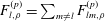 $F_{l,\unicode[STIX]{x1D70C}}^{(p)}=\sum _{m\neq l}F_{lm,\unicode[STIX]{x1D70C}}^{(p)}$
with
$F_{l,\unicode[STIX]{x1D70C}}^{(p)}=\sum _{m\neq l}F_{lm,\unicode[STIX]{x1D70C}}^{(p)}$
with
 $F_{lm,\unicode[STIX]{x1D70C}}^{(p)}$
given by (3.15) in the second equality and
$F_{lm,\unicode[STIX]{x1D70C}}^{(p)}$
given by (3.15) in the second equality and
 $\unicode[STIX]{x1D6E5}_{ij}^{\unicode[STIX]{x1D6FC}\unicode[STIX]{x1D6FD}}:=\unicode[STIX]{x1D6FF}(r_{ij}-d)\hat{r}_{ij,\unicode[STIX]{x1D6FC}}\hat{r}_{ij,\unicode[STIX]{x1D6FD}}\unicode[STIX]{x1D6E9}(-\hat{x}_{ij}{\hat{y}}_{ij})$
(cf. (4.2)). If the particles
$\unicode[STIX]{x1D6E5}_{ij}^{\unicode[STIX]{x1D6FC}\unicode[STIX]{x1D6FD}}:=\unicode[STIX]{x1D6FF}(r_{ij}-d)\hat{r}_{ij,\unicode[STIX]{x1D6FC}}\hat{r}_{ij,\unicode[STIX]{x1D6FD}}\unicode[STIX]{x1D6E9}(-\hat{x}_{ij}{\hat{y}}_{ij})$
(cf. (4.2)). If the particles
 $l,m$
differ from any of the particle
$l,m$
differ from any of the particle
 $i$
,
$i$
,
 $j$
or
$j$
or
 $k$
, the correlation decouples and vanishes due to
$k$
, the correlation decouples and vanishes due to
 $\langle \tilde{\unicode[STIX]{x1D70E}}_{\unicode[STIX]{x1D70C}\unicode[STIX]{x1D706}}\rangle _{eq}=0$
. Hence, particle
$\langle \tilde{\unicode[STIX]{x1D70E}}_{\unicode[STIX]{x1D70C}\unicode[STIX]{x1D706}}\rangle _{eq}=0$
. Hence, particle
 $l$
or
$l$
or
 $m$
must be equal to at least one of the particles
$m$
must be equal to at least one of the particles
 $i$
,
$i$
,
 $j$
or
$j$
or
 $k$
. Let us choose
$k$
. Let us choose
 $l$
to be equal to
$l$
to be equal to
 $i$
, and redefine
$i$
, and redefine
 $m$
as
$m$
as
 $l$
,
$l$
,
 $$\begin{eqnarray}\displaystyle & & \displaystyle \frac{V}{2T}\unicode[STIX]{x1D6F1}_{\unicode[STIX]{x1D70C}\unicode[STIX]{x1D706}}\mathop{\sum }_{i=1}^{N}\mathop{\sum }_{j\neq i}\mathop{\sum }_{k\neq i}\langle \unicode[STIX]{x1D6E5}_{ij}^{xy}\unicode[STIX]{x1D6E5}_{ik}^{xy}\hat{r}_{ij,\unicode[STIX]{x1D6FC}}\hat{r}_{ik,\unicode[STIX]{x1D6FD}}\tilde{\unicode[STIX]{x1D70E}}_{\unicode[STIX]{x1D70C}\unicode[STIX]{x1D706}}\rangle _{eq}+(\unicode[STIX]{x1D6FC}\leftrightarrow \unicode[STIX]{x1D6FD})\nonumber\\ \displaystyle & & \displaystyle \quad =-\frac{\unicode[STIX]{x1D701}\dot{\unicode[STIX]{x1D6FE}}d^{2}}{2T}\unicode[STIX]{x1D6F1}_{\unicode[STIX]{x1D70C}\unicode[STIX]{x1D706}}\mathop{\sum }_{i=1}^{N}\mathop{\sum }_{j\neq i}\mathop{\sum }_{k\neq i}\mathop{\sum }_{l}\langle \unicode[STIX]{x1D6E5}_{ij}^{xy}\unicode[STIX]{x1D6E5}_{ik}^{xy}\unicode[STIX]{x1D6E5}_{il}^{xy}\hat{r}_{ij,\unicode[STIX]{x1D6FC}}\hat{r}_{ik,\unicode[STIX]{x1D6FD}}r_{i,\unicode[STIX]{x1D706}}\hat{r}_{il,\unicode[STIX]{x1D70C}}\rangle _{eq}+(\unicode[STIX]{x1D6FC}\leftrightarrow \unicode[STIX]{x1D6FD}).\qquad\end{eqnarray}$$
This term includes four indices
 $i,j,k,l$
for the particles, and can be decomposed into four-, three- and two-body correlations.
$i,j,k,l$
for the particles, and can be decomposed into four-, three- and two-body correlations.
The four-body correlation corresponds to the case where all the indices
 $i,j,k,l$
are different from one another. It can be expressed by the quadruplet-correlation function
$i,j,k,l$
are different from one another. It can be expressed by the quadruplet-correlation function
 $g^{(4)}(\boldsymbol{r},\boldsymbol{r}^{\prime },\boldsymbol{r}^{\prime \prime })$
, equation (4.18), as
$g^{(4)}(\boldsymbol{r},\boldsymbol{r}^{\prime },\boldsymbol{r}^{\prime \prime })$
, equation (4.18), as
 $$\begin{eqnarray}\displaystyle & & \displaystyle (\text{four-body correlation})\nonumber\\ \displaystyle & & \displaystyle \quad =-\frac{\unicode[STIX]{x1D701}\dot{\unicode[STIX]{x1D6FE}}d^{3}}{4T}\unicode[STIX]{x1D6F1}_{\unicode[STIX]{x1D70C}\unicode[STIX]{x1D706}}\sum _{i,j,k,l}\langle \unicode[STIX]{x1D6E5}_{ij}^{xy}\unicode[STIX]{x1D6E5}_{ik}^{xy}\unicode[STIX]{x1D6E5}_{il}^{xy}\hat{r}_{ij,\unicode[STIX]{x1D6FC}}\hat{r}_{ik,\unicode[STIX]{x1D6FD}}\hat{r}_{il,\unicode[STIX]{x1D706}}\hat{r}_{il,\unicode[STIX]{x1D70C}}\rangle _{eq}+(\unicode[STIX]{x1D6FC}\leftrightarrow \unicode[STIX]{x1D6FD})\nonumber\\ \displaystyle & & \displaystyle \quad =-N\frac{\unicode[STIX]{x1D701}\dot{\unicode[STIX]{x1D6FE}}d^{3}}{4T}\unicode[STIX]{x1D6F1}_{\unicode[STIX]{x1D70C}\unicode[STIX]{x1D706}}n(\unicode[STIX]{x1D711})^{3}\int \text{d}^{3}\boldsymbol{r}\int \text{d}^{3}\boldsymbol{r}^{\prime }\int \text{d}^{3}\boldsymbol{r}^{\prime \prime }\,g^{(4)}(\boldsymbol{r},\boldsymbol{r}^{\prime },\boldsymbol{r}^{\prime \prime })\unicode[STIX]{x1D6FF}(r-d)\unicode[STIX]{x1D6FF}(r^{\prime }-d)\unicode[STIX]{x1D6FF}(r^{\prime \prime }-d)\nonumber\\ \displaystyle & & \displaystyle \qquad \times \,\hat{r}_{\unicode[STIX]{x1D6FC}}\hat{r}_{\unicode[STIX]{x1D6FD}}^{\,\prime }\hat{r}_{\unicode[STIX]{x1D706}}^{\,\prime \prime }\hat{r}_{\unicode[STIX]{x1D70C}}^{\,\prime \prime }\hat{x}{\hat{y}}\unicode[STIX]{x1D6E9}_{\hat{r}}\hat{x}^{\prime }{\hat{y}}^{\prime }\unicode[STIX]{x1D6E9}_{\hat{r}^{\prime }}\hat{x}^{\prime \prime }{\hat{y}}^{\prime \prime }\unicode[STIX]{x1D6E9}_{\hat{r}^{\prime \prime }}+(\unicode[STIX]{x1D6FC}\leftrightarrow \unicode[STIX]{x1D6FD}),\end{eqnarray}$$
where the summation
 $\sum _{i,j,k,l}^{\prime \prime \prime }$
is performed over
$\sum _{i,j,k,l}^{\prime \prime \prime }$
is performed over
 $(i,j,k,l)$
with all the indices different from one other. Note that
$(i,j,k,l)$
with all the indices different from one other. Note that
 $r_{i,\unicode[STIX]{x1D706}}$
is converted to
$r_{i,\unicode[STIX]{x1D706}}$
is converted to
 $r_{il,\unicode[STIX]{x1D706}}$
by virtue of the odd parity with respect to the exchange
$r_{il,\unicode[STIX]{x1D706}}$
by virtue of the odd parity with respect to the exchange
 $i\leftrightarrow l$
. This conversion allows us to express this term only in relative coordinates.
$i\leftrightarrow l$
. This conversion allows us to express this term only in relative coordinates.
The three-body correlation is obtained by setting
 $l$
equal to
$l$
equal to
 $j$
or
$j$
or
 $k$
in (B 6). Let us choose
$k$
in (B 6). Let us choose
 $l$
to be equal to
$l$
to be equal to
 $j$
,
$j$
,
 $$\begin{eqnarray}\displaystyle & & \displaystyle (\text{three-body correlation})\nonumber\\ \displaystyle & & \displaystyle \quad =-\frac{\unicode[STIX]{x1D701}\dot{\unicode[STIX]{x1D6FE}}d}{2T}\unicode[STIX]{x1D6F1}_{\unicode[STIX]{x1D70C}\unicode[STIX]{x1D706}}\sum _{i,j,k}\langle \tilde{\unicode[STIX]{x1D6E5}}_{ij}\unicode[STIX]{x1D6E5}_{ik}^{xy}\hat{r}_{ij,\unicode[STIX]{x1D6FC}}\hat{r}_{ik,\unicode[STIX]{x1D6FD}}r_{i,\unicode[STIX]{x1D706}}\hat{r}_{ij,\unicode[STIX]{x1D70C}}\hat{x}_{ij}^{2}{\hat{y}}_{ij}^{2}\unicode[STIX]{x1D6E9}_{ij}\rangle _{eq}+(\unicode[STIX]{x1D6FC}\leftrightarrow \unicode[STIX]{x1D6FD}).\end{eqnarray}$$
Here,
 $r_{i,\unicode[STIX]{x1D706}}$
should be converted to
$r_{i,\unicode[STIX]{x1D706}}$
should be converted to
 $r_{ij,\unicode[STIX]{x1D706}}$
or
$r_{ij,\unicode[STIX]{x1D706}}$
or
 $r_{ik,\unicode[STIX]{x1D706}}$
, in order for this term to be expressed only in relative coordinates. By noting that this term is even with respect to the exchange
$r_{ik,\unicode[STIX]{x1D706}}$
, in order for this term to be expressed only in relative coordinates. By noting that this term is even with respect to the exchange
 $i\leftrightarrow j$
and odd with respect to
$i\leftrightarrow j$
and odd with respect to
 $i\leftrightarrow k$
,
$i\leftrightarrow k$
,
 $r_{ij,\unicode[STIX]{x1D706}}$
vanishes and
$r_{ij,\unicode[STIX]{x1D706}}$
vanishes and
 $r_{ik,\unicode[STIX]{x1D706}}$
survives. Hence, we obtain
$r_{ik,\unicode[STIX]{x1D706}}$
survives. Hence, we obtain
 $$\begin{eqnarray}\displaystyle & & \displaystyle (\text{three-body correlation})\nonumber\\ \displaystyle & & \displaystyle \quad =-\frac{\unicode[STIX]{x1D701}\dot{\unicode[STIX]{x1D6FE}}d^{2}}{4T}\unicode[STIX]{x1D6F1}_{\unicode[STIX]{x1D70C}\unicode[STIX]{x1D706}}\sum _{i,j,k}\langle \tilde{\unicode[STIX]{x1D6E5}}_{ij}\unicode[STIX]{x1D6E5}_{ik}^{xy}\hat{r}_{ij,\unicode[STIX]{x1D6FC}}\hat{r}_{ij,\unicode[STIX]{x1D70C}}\hat{r}_{ik,\unicode[STIX]{x1D6FD}}\hat{r}_{ik,\unicode[STIX]{x1D706}}\hat{x}_{ij}^{2}{\hat{y}}_{ij}^{2}\unicode[STIX]{x1D6E9}_{ij}\rangle _{eq}+(\unicode[STIX]{x1D6FC}\leftrightarrow \unicode[STIX]{x1D6FD})\nonumber\\ \displaystyle & & \displaystyle \quad =-N\frac{\unicode[STIX]{x1D701}\dot{\unicode[STIX]{x1D6FE}}d^{2}}{4T}\unicode[STIX]{x1D6F1}_{\unicode[STIX]{x1D70C}\unicode[STIX]{x1D706}}n(\unicode[STIX]{x1D711})^{2}\int \text{d}^{3}\boldsymbol{r}\int \text{d}^{3}\boldsymbol{r}^{\prime }\,g^{(3)}(\boldsymbol{r},\boldsymbol{r}^{\prime })\unicode[STIX]{x1D6FF}(r-d)\unicode[STIX]{x1D6FF}(r^{\prime }-d)\hat{r}_{\unicode[STIX]{x1D6FC}}\hat{r}_{\unicode[STIX]{x1D70C}}\hat{r}_{\unicode[STIX]{x1D6FD}}^{\prime }\hat{r}_{\unicode[STIX]{x1D706}}^{\prime }\hat{x}^{2}{\hat{y}}^{2}\unicode[STIX]{x1D6E9}_{\hat{r}}\hat{x}^{\prime }{\hat{y}}^{\prime }\unicode[STIX]{x1D6E9}_{\hat{r}^{\prime }}\nonumber\\ \displaystyle & & \displaystyle \qquad +\,(\unicode[STIX]{x1D6FC}\leftrightarrow \unicode[STIX]{x1D6FD}).\end{eqnarray}$$
Finally, the two-body correlation is obtained by setting
 $k=j$
in the expression for the three-body correlation. This is given by
$k=j$
in the expression for the three-body correlation. This is given by
 $$\begin{eqnarray}\displaystyle & & \displaystyle (\text{two-body correlation})\nonumber\\ \displaystyle & & \displaystyle \quad =-\frac{\unicode[STIX]{x1D701}\dot{\unicode[STIX]{x1D6FE}}d}{4T}\unicode[STIX]{x1D6F1}_{\unicode[STIX]{x1D70C}\unicode[STIX]{x1D706}}\sum _{i,j}\langle \tilde{\unicode[STIX]{x1D6E5}}_{ij}\hat{r}_{ij,\unicode[STIX]{x1D6FC}}\hat{r}_{ij,\unicode[STIX]{x1D6FD}}\hat{r}_{ij,\unicode[STIX]{x1D70C}}\hat{r}_{ij,\unicode[STIX]{x1D706}}\hat{x}_{ij}^{3}{\hat{y}}_{ij}^{3}\unicode[STIX]{x1D6E9}_{ij}\rangle _{eq}+(\unicode[STIX]{x1D6FC}\leftrightarrow \unicode[STIX]{x1D6FD})\nonumber\\ \displaystyle & & \displaystyle \quad =-N\frac{\unicode[STIX]{x1D701}\dot{\unicode[STIX]{x1D6FE}}d}{4T}\unicode[STIX]{x1D6F1}_{\unicode[STIX]{x1D70C}\unicode[STIX]{x1D706}}n(\unicode[STIX]{x1D711})\int \text{d}^{3}\boldsymbol{r}g(r)\unicode[STIX]{x1D6FF}(r-d)\hat{r}_{\unicode[STIX]{x1D6FC}}\hat{r}_{\unicode[STIX]{x1D6FD}}\hat{r}_{\unicode[STIX]{x1D70C}}\hat{r}_{\unicode[STIX]{x1D706}}\hat{x}^{3}{\hat{y}}^{3}\unicode[STIX]{x1D6E9}_{\hat{r}}+(\unicode[STIX]{x1D6FC}\leftrightarrow \unicode[STIX]{x1D6FD})\nonumber\\ \displaystyle & & \displaystyle \quad =-N\frac{\unicode[STIX]{x1D701}\dot{\unicode[STIX]{x1D6FE}}d}{2T}\unicode[STIX]{x1D6F1}_{\unicode[STIX]{x1D70C}\unicode[STIX]{x1D706}}n(\unicode[STIX]{x1D711})\int \text{d}^{3}\boldsymbol{r}g(r)\unicode[STIX]{x1D6FF}(r-d)\hat{r}_{\unicode[STIX]{x1D6FC}}\hat{r}_{\unicode[STIX]{x1D6FD}}\hat{r}_{\unicode[STIX]{x1D70C}}\hat{r}_{\unicode[STIX]{x1D706}}\hat{x}^{3}{\hat{y}}^{3}\unicode[STIX]{x1D6E9}_{\hat{r}}.\end{eqnarray}$$
From (B 6), (B 8) and (B 9), we obtain
 $$\begin{eqnarray}\displaystyle & & \displaystyle \frac{V}{2T}\unicode[STIX]{x1D6F1}_{\unicode[STIX]{x1D70C}\unicode[STIX]{x1D706}}\mathop{\sum }_{i=1}^{N}\mathop{\sum }_{j\neq i}\mathop{\sum }_{k\neq i}\langle \unicode[STIX]{x1D6E5}_{ij}^{xy}\unicode[STIX]{x1D6E5}_{ik}^{xy}\hat{r}_{ij,\unicode[STIX]{x1D6FC}}\hat{r}_{ik,\unicode[STIX]{x1D6FD}}\tilde{\unicode[STIX]{x1D70E}}_{\unicode[STIX]{x1D70C}\unicode[STIX]{x1D706}}\rangle _{eq}+(\unicode[STIX]{x1D6FC}\leftrightarrow \unicode[STIX]{x1D6FD})\nonumber\\ \displaystyle & & \displaystyle \quad \approx \,-N\frac{\unicode[STIX]{x1D701}\dot{\unicode[STIX]{x1D6FE}}d^{3}}{4T}\unicode[STIX]{x1D6F1}_{\unicode[STIX]{x1D70C}\unicode[STIX]{x1D706}}n(\unicode[STIX]{x1D711})^{3}\int \text{d}^{3}\boldsymbol{r}\int \text{d}^{3}\boldsymbol{r}^{\prime }\int \text{d}^{3}\boldsymbol{r}^{\prime \prime }g^{(4)}(\boldsymbol{r},\boldsymbol{r}^{\prime },\boldsymbol{r}^{\prime \prime })\unicode[STIX]{x1D6FF}(r-d)\unicode[STIX]{x1D6FF}(r^{\prime }-d)\unicode[STIX]{x1D6FF}(r^{\prime \prime }-d)\nonumber\\ \displaystyle & & \displaystyle \qquad \times \,\hat{r}_{\unicode[STIX]{x1D6FC}}\hat{r}_{\unicode[STIX]{x1D6FD}}^{\prime }\hat{r}_{\unicode[STIX]{x1D706}}^{\prime \prime }\hat{r}_{\unicode[STIX]{x1D70C}}^{\prime \prime }\hat{x}{\hat{y}}\unicode[STIX]{x1D6E9}_{\hat{r}}\hat{x}^{\prime }{\hat{y}}^{\prime }\unicode[STIX]{x1D6E9}_{\hat{r}^{\prime }}\hat{x}^{\prime \prime }{\hat{y}}^{\prime \prime }\unicode[STIX]{x1D6E9}_{\hat{r}^{\prime \prime }}+(\unicode[STIX]{x1D6FC}\leftrightarrow \unicode[STIX]{x1D6FD})\nonumber\\ \displaystyle & & \displaystyle \qquad -\,N\frac{\unicode[STIX]{x1D701}\dot{\unicode[STIX]{x1D6FE}}d^{2}}{4T}\unicode[STIX]{x1D6F1}_{\unicode[STIX]{x1D70C}\unicode[STIX]{x1D706}}n(\unicode[STIX]{x1D711})^{2}\nonumber\\ \displaystyle & & \displaystyle \times \,\int \text{d}^{3}\boldsymbol{r}\int \text{d}^{3}\boldsymbol{r}^{\prime }g^{(3)}(\boldsymbol{r},\boldsymbol{r}^{\prime })\unicode[STIX]{x1D6FF}(r-d)\unicode[STIX]{x1D6FF}(r^{\prime }-d)\hat{r}_{\unicode[STIX]{x1D6FC}}\hat{r}_{\unicode[STIX]{x1D70C}}\hat{r}_{\unicode[STIX]{x1D6FD}}^{\prime }\hat{r}_{\unicode[STIX]{x1D706}}^{\prime }\hat{x}^{2}{\hat{y}}^{2}\unicode[STIX]{x1D6E9}_{\hat{r}}\hat{x}^{\prime }{\hat{y}}^{\prime }\unicode[STIX]{x1D6E9}_{\hat{r}^{\prime }}+(\unicode[STIX]{x1D6FC}\leftrightarrow \unicode[STIX]{x1D6FD})\nonumber\\ \displaystyle & & \displaystyle \qquad -\,N\frac{\unicode[STIX]{x1D701}\dot{\unicode[STIX]{x1D6FE}}d}{2T}\unicode[STIX]{x1D6F1}_{\unicode[STIX]{x1D70C}\unicode[STIX]{x1D706}}n(\unicode[STIX]{x1D711})\int \text{d}^{3}\boldsymbol{r}\,g(r)\unicode[STIX]{x1D6FF}(r-d)\hat{r}_{\unicode[STIX]{x1D6FC}}\hat{r}_{\unicode[STIX]{x1D6FD}}\hat{r}_{\unicode[STIX]{x1D70C}}\hat{r}_{\unicode[STIX]{x1D706}}\hat{x}^{3}{\hat{y}}^{3}\unicode[STIX]{x1D6E9}_{\hat{r}}.\end{eqnarray}$$
Similarly, the canonical term for the second term on the right-hand side of (4.5) is given by
 $$\begin{eqnarray}\displaystyle & & \displaystyle \frac{V}{2T}\unicode[STIX]{x1D6F1}_{\unicode[STIX]{x1D70C}\unicode[STIX]{x1D706}}\mathop{\sum }_{i=1}^{N}\mathop{\sum }_{j\neq i}\mathop{\sum }_{k\neq i}\langle \unicode[STIX]{x1D6E5}_{ij}^{\unicode[STIX]{x1D6FC}\unicode[STIX]{x1D6FD}}\unicode[STIX]{x1D6E5}_{ik}^{xy}(\hat{x}_{ij}{\hat{y}}_{ik}+{\hat{y}}_{ij}\hat{x}_{ik})\tilde{\unicode[STIX]{x1D70E}}_{\unicode[STIX]{x1D70C}\unicode[STIX]{x1D706}}\rangle _{eq}\nonumber\\ \displaystyle & & \displaystyle \quad \approx \,-N\frac{\unicode[STIX]{x1D701}\dot{\unicode[STIX]{x1D6FE}}d^{3}}{4T}\unicode[STIX]{x1D6F1}_{\unicode[STIX]{x1D70C}\unicode[STIX]{x1D706}}n(\unicode[STIX]{x1D711})^{3}\int \text{d}^{3}\boldsymbol{r}\int \text{d}^{3}\boldsymbol{r}^{\prime }\int \text{d}^{3}\boldsymbol{r}^{\prime \prime }g^{(4)}(\boldsymbol{r},\boldsymbol{r}^{\prime },\boldsymbol{r}^{\prime \prime })\unicode[STIX]{x1D6FF}(r-d)\unicode[STIX]{x1D6FF}(r^{\prime }-d)\unicode[STIX]{x1D6FF}(r^{\prime \prime }-d)\nonumber\\ \displaystyle & & \displaystyle \qquad \times \,(\hat{x}{\hat{y}}^{\prime }+{\hat{y}}\hat{x}^{\prime })\hat{r}_{\unicode[STIX]{x1D706}}^{\prime \prime }\hat{r}_{\unicode[STIX]{x1D70C}}^{\prime \prime }\hat{r}_{\unicode[STIX]{x1D6FC}}\hat{r}_{\unicode[STIX]{x1D6FD}}\unicode[STIX]{x1D6E9}_{\hat{r}}\hat{x}^{\prime }{\hat{y}}^{\prime }\unicode[STIX]{x1D6E9}_{\hat{r}^{\prime }}\hat{x}^{\prime \prime }{\hat{y}}^{\prime \prime }\unicode[STIX]{x1D6E9}_{\hat{r}^{\prime \prime }}+(\unicode[STIX]{x1D6FC}\leftrightarrow \unicode[STIX]{x1D6FD})\nonumber\\ \displaystyle & & \displaystyle \qquad -\,N\frac{\unicode[STIX]{x1D701}\dot{\unicode[STIX]{x1D6FE}}d^{2}}{4T}\unicode[STIX]{x1D6F1}_{\unicode[STIX]{x1D70C}\unicode[STIX]{x1D706}}n(\unicode[STIX]{x1D711})^{2}\nonumber\\ \displaystyle & & \displaystyle \qquad \times \,\int \text{d}^{3}\boldsymbol{r}\int \text{d}^{3}\boldsymbol{r}^{\prime }g^{(3)}(\boldsymbol{r},\boldsymbol{r}^{\prime })\unicode[STIX]{x1D6FF}(r-d)\unicode[STIX]{x1D6FF}(r^{\prime }-d)(\hat{x}{\hat{y}}^{\prime }+{\hat{y}}\hat{x}^{\prime })\hat{r}_{\unicode[STIX]{x1D70C}}\hat{r}_{\unicode[STIX]{x1D706}}^{\prime }\hat{x}{\hat{y}}\hat{r}_{\unicode[STIX]{x1D6FC}}\hat{r}_{\unicode[STIX]{x1D6FD}}\unicode[STIX]{x1D6E9}_{\hat{r}}\hat{x}^{\prime }{\hat{y}}^{\prime }\unicode[STIX]{x1D6E9}_{\hat{r}^{\prime }}\nonumber\\ \displaystyle & & \displaystyle \qquad -\,N\frac{\unicode[STIX]{x1D701}\dot{\unicode[STIX]{x1D6FE}}d}{2T}\unicode[STIX]{x1D6F1}_{\unicode[STIX]{x1D70C}\unicode[STIX]{x1D706}}n(\unicode[STIX]{x1D711})\int \text{d}^{3}\boldsymbol{r}g(r)\unicode[STIX]{x1D6FF}(r-d)\hat{r}_{\unicode[STIX]{x1D6FC}}\hat{r}_{\unicode[STIX]{x1D6FD}}\hat{r}_{\unicode[STIX]{x1D70C}}\hat{r}_{\unicode[STIX]{x1D706}}\hat{x}^{3}{\hat{y}}^{3}\unicode[STIX]{x1D6E9}_{\hat{r}}.\end{eqnarray}$$
B.2 Factorization approximation
The first and second terms on the right-hand side of (4.5) are expressed as spatial integrations of the correlation functions
 $g^{(4)}(\boldsymbol{r},\boldsymbol{r}^{\prime },\boldsymbol{r}^{\prime \prime })$
,
$g^{(4)}(\boldsymbol{r},\boldsymbol{r}^{\prime },\boldsymbol{r}^{\prime \prime })$
,
 $g^{(3)}(\boldsymbol{r},\boldsymbol{r}^{\prime })$
and
$g^{(3)}(\boldsymbol{r},\boldsymbol{r}^{\prime })$
and
 $g(r)$
by means of the approximate formula (4.9), as is shown in (B 2), (B 3), (B 10) and (B 11). To proceed, it is necessary to adopt approximations for
$g(r)$
by means of the approximate formula (4.9), as is shown in (B 2), (B 3), (B 10) and (B 11). To proceed, it is necessary to adopt approximations for
 $g^{(4)}(\boldsymbol{r},\boldsymbol{r}^{\prime },\boldsymbol{r}^{\prime \prime })$
and
$g^{(4)}(\boldsymbol{r},\boldsymbol{r}^{\prime },\boldsymbol{r}^{\prime \prime })$
and
 $g^{(3)}(\boldsymbol{r},\boldsymbol{r}^{\prime })$
, which are difficult to evaluate. As explained in § 4.2, we adopt the following approximations which are valid for the evaluation of divergences in the vicinity of the jamming point,
$g^{(3)}(\boldsymbol{r},\boldsymbol{r}^{\prime })$
, which are difficult to evaluate. As explained in § 4.2, we adopt the following approximations which are valid for the evaluation of divergences in the vicinity of the jamming point,
 $$\begin{eqnarray}\displaystyle & \displaystyle g^{(4)}(\boldsymbol{r},\boldsymbol{r}^{\prime },\boldsymbol{r}^{\prime \prime })\approx g(r)g(r^{\prime })g(r^{\prime \prime })\quad (r,r^{\prime },r^{\prime \prime }\approx d), & \displaystyle\end{eqnarray}$$
 $$\begin{eqnarray}\displaystyle & \displaystyle g^{(3)}(\boldsymbol{r},\boldsymbol{r}^{\prime })\approx g(r)g(r^{\prime })\quad (r,r^{\prime }\approx d). & \displaystyle\end{eqnarray}$$
We apply (B 12) and (B 13) to (B 2), (B 3), (B 10) and (B 11), and utilize
 $g(r)\unicode[STIX]{x1D6FF}(r-d)=g_{0}(\unicode[STIX]{x1D711})\unicode[STIX]{x1D6FF}(r-d)$
in this section.
$g(r)\unicode[STIX]{x1D6FF}(r-d)=g_{0}(\unicode[STIX]{x1D711})\unicode[STIX]{x1D6FF}(r-d)$
in this section.
B.2.1 Canonical terms
By applying (B 13) to (B 2), the radial integrations can be performed straightforwardly. Thus we obtain
 $$\begin{eqnarray}\displaystyle & & \displaystyle \mathop{\sum }_{i=1}^{N}\mathop{\sum }_{j\neq i}\mathop{\sum }_{k\neq i}\langle \unicode[STIX]{x1D6E5}_{ij}^{xy}\unicode[STIX]{x1D6E5}_{ik}^{xy}(\hat{r}_{ij,\unicode[STIX]{x1D6FC}}\hat{r}_{ik,\unicode[STIX]{x1D6FD}}+\hat{r}_{ij,\unicode[STIX]{x1D6FD}}\hat{r}_{ik,\unicode[STIX]{x1D6FC}})\rangle _{eq}\nonumber\\ \displaystyle & & \displaystyle \quad \approx \,\frac{N}{d^{2}}\unicode[STIX]{x1D711}^{\ast 2}g_{0}(\unicode[STIX]{x1D711})^{2}\int \text{d}{\mathcal{S}}\int \text{d}{\mathcal{S}}^{\prime }(\hat{r}_{\unicode[STIX]{x1D6FC}}\hat{r}_{\unicode[STIX]{x1D6FD}}^{\prime }+\hat{r}_{\unicode[STIX]{x1D6FD}}\hat{r}_{\unicode[STIX]{x1D6FC}}^{\prime })\hat{x}{\hat{y}}\unicode[STIX]{x1D6E9}_{\hat{r}}\hat{x}^{\prime }{\hat{y}}^{\prime }\unicode[STIX]{x1D6E9}_{\hat{r}^{\prime }}+2\frac{N}{d^{2}}\unicode[STIX]{x1D711}^{\ast }g_{0}(\unicode[STIX]{x1D711})\nonumber\\ \displaystyle & & \displaystyle \qquad \times \,\int \text{d}{\mathcal{S}}\hat{r}_{\unicode[STIX]{x1D6FC}}\hat{r}_{\unicode[STIX]{x1D6FD}}\hat{x}^{2}{\hat{y}}^{2}\unicode[STIX]{x1D6E9}_{\hat{r}}\nonumber\\ \displaystyle & & \displaystyle \quad =\frac{N}{d^{2}}\{\unicode[STIX]{x1D711}^{\ast 2}g_{0}(\unicode[STIX]{x1D711})^{2}{\mathcal{S}}_{\unicode[STIX]{x1D6FC}\unicode[STIX]{x1D6FD}}^{(1:c2)}+\unicode[STIX]{x1D711}^{\ast }g_{0}(\unicode[STIX]{x1D711}){\mathcal{S}}_{\unicode[STIX]{x1D6FC}\unicode[STIX]{x1D6FD}}^{(1:c1)}\},\end{eqnarray}$$
where
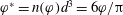 $\unicode[STIX]{x1D711}^{\ast }=n(\unicode[STIX]{x1D711})d^{3}=6\unicode[STIX]{x1D711}/\unicode[STIX]{x03C0}$
is the dimensionless average number density and the angular integrals
$\unicode[STIX]{x1D711}^{\ast }=n(\unicode[STIX]{x1D711})d^{3}=6\unicode[STIX]{x1D711}/\unicode[STIX]{x03C0}$
is the dimensionless average number density and the angular integrals
 ${\mathcal{S}}_{\unicode[STIX]{x1D6FC}\unicode[STIX]{x1D6FD}}^{(1:c2)}$
and
${\mathcal{S}}_{\unicode[STIX]{x1D6FC}\unicode[STIX]{x1D6FD}}^{(1:c2)}$
and
 ${\mathcal{S}}_{\unicode[STIX]{x1D6FC}\unicode[STIX]{x1D6FD}}^{(1:c1)}$
are given by
${\mathcal{S}}_{\unicode[STIX]{x1D6FC}\unicode[STIX]{x1D6FD}}^{(1:c1)}$
are given by
 $$\begin{eqnarray}\displaystyle & \displaystyle {\mathcal{S}}_{\unicode[STIX]{x1D6FC}\unicode[STIX]{x1D6FD}}^{(1:c2)}=\int \text{d}{\mathcal{S}}\int \text{d}{\mathcal{S}}^{\prime }\,\hat{x}{\hat{y}}\hat{x}^{\prime }{\hat{y}}^{\prime }(\hat{r}_{\unicode[STIX]{x1D6FC}}\hat{r}_{\unicode[STIX]{x1D6FD}}^{\prime }+\hat{r}_{\unicode[STIX]{x1D6FD}}\hat{r}_{\unicode[STIX]{x1D6FC}}^{\prime })\unicode[STIX]{x1D6E9}_{\hat{r}}\unicode[STIX]{x1D6E9}_{\hat{r}^{\prime }}, & \displaystyle\end{eqnarray}$$
 $$\begin{eqnarray}\displaystyle & \displaystyle {\mathcal{S}}_{\unicode[STIX]{x1D6FC}\unicode[STIX]{x1D6FD}}^{(1:c1)}=2\int \text{d}{\mathcal{S}}\hat{x}^{2}{\hat{y}}^{2}\hat{r}_{\unicode[STIX]{x1D6FC}}\hat{r}_{\unicode[STIX]{x1D6FD}}\unicode[STIX]{x1D6E9}_{\hat{r}}. & \displaystyle\end{eqnarray}$$
Here,
 $\int \text{d}{\mathcal{S}}\cdots \,$
and
$\int \text{d}{\mathcal{S}}\cdots \,$
and
 $\int \text{d}{\mathcal{S}}^{\prime }\cdots \,$
are angular integrals with respect to
$\int \text{d}{\mathcal{S}}^{\prime }\cdots \,$
are angular integrals with respect to
 $\hat{\boldsymbol{r}}$
and
$\hat{\boldsymbol{r}}$
and
 $\hat{\boldsymbol{r}}^{\prime }$
, respectively. Equation (B 3) can be evaluated similarly. The result is synthesized as follows,
$\hat{\boldsymbol{r}}^{\prime }$
, respectively. Equation (B 3) can be evaluated similarly. The result is synthesized as follows,
 $$\begin{eqnarray}(\text{canonical})=-\frac{\unicode[STIX]{x1D701}\dot{\unicode[STIX]{x1D6FE}}}{4d}\mathop{\sum }_{\ell =1}^{2}\{\unicode[STIX]{x1D711}^{\ast 3}g_{0}(\unicode[STIX]{x1D711})^{2}{\mathcal{S}}_{\unicode[STIX]{x1D6FC}\unicode[STIX]{x1D6FD}}^{(\ell :c2)}+\unicode[STIX]{x1D711}^{\ast 2}g_{0}(\unicode[STIX]{x1D711}){\mathcal{S}}_{\unicode[STIX]{x1D6FC}\unicode[STIX]{x1D6FD}}^{(\ell :c1)}\},\end{eqnarray}$$
where the angular integrals
 ${\mathcal{S}}_{\unicode[STIX]{x1D6FC}\unicode[STIX]{x1D6FD}}^{(2:c2)}$
,
${\mathcal{S}}_{\unicode[STIX]{x1D6FC}\unicode[STIX]{x1D6FD}}^{(2:c2)}$
,
 ${\mathcal{S}}_{\unicode[STIX]{x1D6FC}\unicode[STIX]{x1D6FD}}^{(2:c1)}$
are given by
${\mathcal{S}}_{\unicode[STIX]{x1D6FC}\unicode[STIX]{x1D6FD}}^{(2:c1)}$
are given by
 $$\begin{eqnarray}\displaystyle & \displaystyle {\mathcal{S}}_{\unicode[STIX]{x1D6FC}\unicode[STIX]{x1D6FD}}^{(2:c2)}=\int \text{d}{\mathcal{S}}\int \text{d}{\mathcal{S}}^{\prime }\hat{r}_{\unicode[STIX]{x1D6FC}}\hat{r}_{\unicode[STIX]{x1D6FD}}\hat{x}^{\prime }{\hat{y}}^{\prime }(\hat{x}{\hat{y}}^{\prime }+{\hat{y}}\hat{x}^{\prime })\unicode[STIX]{x1D6E9}_{\hat{r}}\unicode[STIX]{x1D6E9}_{\hat{r}^{\prime }}, & \displaystyle\end{eqnarray}$$
 $$\begin{eqnarray}\displaystyle & \displaystyle {\mathcal{S}}_{\unicode[STIX]{x1D6FC}\unicode[STIX]{x1D6FD}}^{(2:c1)}={\mathcal{S}}_{\unicode[STIX]{x1D6FC}\unicode[STIX]{x1D6FD}}^{(1:c1)}. & \displaystyle\end{eqnarray}$$
B.2.2 Non-canonical terms
By applying (B 12) and (B 13) to (B 10), the radial integrations can be performed straightforwardly. Thus we obtain
 $$\begin{eqnarray}\displaystyle & & \displaystyle \frac{V}{2T}\unicode[STIX]{x1D6F1}_{\unicode[STIX]{x1D70C}\unicode[STIX]{x1D706}}\mathop{\sum }_{i=1}^{N}\mathop{\sum }_{j\neq i}\mathop{\sum }_{k\neq i}\langle \unicode[STIX]{x1D6E5}_{ij}^{xy}\unicode[STIX]{x1D6E5}_{ik}^{xy}\hat{r}_{ij,\unicode[STIX]{x1D6FC}}\hat{r}_{ik,\unicode[STIX]{x1D6FD}}\tilde{\unicode[STIX]{x1D70E}}_{\unicode[STIX]{x1D70C}\unicode[STIX]{x1D706}}\rangle _{eq}+(\unicode[STIX]{x1D6FC}\leftrightarrow \unicode[STIX]{x1D6FD})\nonumber\\ \displaystyle & & \displaystyle \quad \approx \,-N\frac{\unicode[STIX]{x1D701}\dot{\unicode[STIX]{x1D6FE}}}{4T}\unicode[STIX]{x1D6F1}_{\unicode[STIX]{x1D70C}\unicode[STIX]{x1D706}}\unicode[STIX]{x1D711}^{\ast 3}g_{0}(\unicode[STIX]{x1D711})^{3}\nonumber\\ \displaystyle & & \displaystyle \qquad \times \,\int \text{d}{\mathcal{S}}\int \text{d}{\mathcal{S}}^{\prime }\int \text{d}{\mathcal{S}}^{\prime \prime }\hat{r}_{\unicode[STIX]{x1D6FC}}\hat{r}_{\unicode[STIX]{x1D6FD}}^{\prime }\hat{r}_{\unicode[STIX]{x1D706}}^{\prime \prime }\hat{r}_{\unicode[STIX]{x1D70C}}^{\prime \prime }\hat{x}{\hat{y}}\unicode[STIX]{x1D6E9}_{\hat{r}}\hat{x}^{\prime }{\hat{y}}^{\prime }\unicode[STIX]{x1D6E9}_{\hat{r}^{\prime }}\hat{x}^{\prime \prime }{\hat{y}}^{\prime \prime }\unicode[STIX]{x1D6E9}_{\hat{r}^{\prime \prime }}+(\unicode[STIX]{x1D6FC}\leftrightarrow \unicode[STIX]{x1D6FD})\nonumber\\ \displaystyle & & \displaystyle \qquad -\,N\frac{\unicode[STIX]{x1D701}\dot{\unicode[STIX]{x1D6FE}}}{4T}\unicode[STIX]{x1D6F1}_{\unicode[STIX]{x1D70C}\unicode[STIX]{x1D706}}\unicode[STIX]{x1D711}^{\ast 2}g_{0}(\unicode[STIX]{x1D711})^{2}\int \text{d}{\mathcal{S}}\int \text{d}{\mathcal{S}}^{\prime }\hat{r}_{\unicode[STIX]{x1D6FC}}\hat{r}_{\unicode[STIX]{x1D70C}}\hat{r}_{\unicode[STIX]{x1D6FD}}^{\prime }\hat{r}_{\unicode[STIX]{x1D706}}^{\prime }\hat{x}^{2}{\hat{y}}^{2}\unicode[STIX]{x1D6E9}_{\hat{r}}\hat{x}^{\prime }{\hat{y}}^{\prime }\unicode[STIX]{x1D6E9}_{\hat{r}^{\prime }}+(\unicode[STIX]{x1D6FC}\leftrightarrow \unicode[STIX]{x1D6FD})\nonumber\\ \displaystyle & & \displaystyle \qquad -\,N\frac{\unicode[STIX]{x1D701}\dot{\unicode[STIX]{x1D6FE}}}{2T}\unicode[STIX]{x1D6F1}_{\unicode[STIX]{x1D70C}\unicode[STIX]{x1D706}}\unicode[STIX]{x1D711}^{\ast }g_{0}(\unicode[STIX]{x1D711})\int \text{d}{\mathcal{S}}\hat{r}_{\unicode[STIX]{x1D6FC}}\hat{r}_{\unicode[STIX]{x1D6FD}}\hat{r}_{\unicode[STIX]{x1D706}}\hat{r}_{\unicode[STIX]{x1D70C}}\hat{x}^{3}{\hat{y}}^{3}\unicode[STIX]{x1D6E9}_{\hat{r}}\nonumber\\ \displaystyle & & \displaystyle \quad =-N\frac{\unicode[STIX]{x1D701}\dot{\unicode[STIX]{x1D6FE}}}{4T}\unicode[STIX]{x1D6F1}_{\unicode[STIX]{x1D70C}\unicode[STIX]{x1D706}}[\unicode[STIX]{x1D711}^{\ast 3}g_{0}(\unicode[STIX]{x1D711})^{3}{\mathcal{S}}_{\unicode[STIX]{x1D6FC}\unicode[STIX]{x1D6FD}\unicode[STIX]{x1D70C}\unicode[STIX]{x1D706}}^{(1:nc3)}+\unicode[STIX]{x1D711}^{\ast 2}g_{0}(\unicode[STIX]{x1D711})^{2}{\mathcal{S}}_{\unicode[STIX]{x1D6FC}\unicode[STIX]{x1D6FD}\unicode[STIX]{x1D70C}\unicode[STIX]{x1D706}}^{(1:nc2)}+\unicode[STIX]{x1D711}^{\ast }g_{0}(\unicode[STIX]{x1D711}){\mathcal{S}}_{\unicode[STIX]{x1D6FC}\unicode[STIX]{x1D6FD}\unicode[STIX]{x1D70C}\unicode[STIX]{x1D706}}^{(1:nc1)}].\end{eqnarray}$$
Here, the angular integrals are given by
 $$\begin{eqnarray}\displaystyle & \displaystyle {\mathcal{S}}_{\unicode[STIX]{x1D6FC}\unicode[STIX]{x1D6FD}\unicode[STIX]{x1D70C}\unicode[STIX]{x1D706}}^{(1:nc3)}=\int \text{d}{\mathcal{S}}\int \text{d}{\mathcal{S}}^{\prime }\int \text{d}{\mathcal{S}}^{\prime \prime }\hat{r}_{\unicode[STIX]{x1D6FC}}\hat{r}_{\unicode[STIX]{x1D6FD}}^{\prime }\hat{r}_{\unicode[STIX]{x1D706}}^{\prime \prime }\hat{r}_{\unicode[STIX]{x1D70C}}^{\prime \prime }\hat{x}{\hat{y}}\unicode[STIX]{x1D6E9}_{\hat{r}}\hat{x}^{\prime }{\hat{y}}^{\prime }\unicode[STIX]{x1D6E9}_{\hat{r}^{\prime }}\hat{x}^{\prime \prime }{\hat{y}}^{\prime \prime }\unicode[STIX]{x1D6E9}_{\hat{r}^{\prime \prime }}+(\unicode[STIX]{x1D6FC}\leftrightarrow \unicode[STIX]{x1D6FD}), & \displaystyle\end{eqnarray}$$
 $$\begin{eqnarray}\displaystyle & \displaystyle {\mathcal{S}}_{\unicode[STIX]{x1D6FC}\unicode[STIX]{x1D6FD}\unicode[STIX]{x1D70C}\unicode[STIX]{x1D706}}^{(1:nc2)}=\int \text{d}{\mathcal{S}}\int \text{d}{\mathcal{S}}^{\prime }\hat{r}_{\unicode[STIX]{x1D6FC}}\hat{r}_{\unicode[STIX]{x1D70C}}\hat{r}_{\unicode[STIX]{x1D6FD}}^{\prime }\hat{r}_{\unicode[STIX]{x1D706}}^{\prime }\hat{x}^{2}{\hat{y}}^{2}\unicode[STIX]{x1D6E9}_{\hat{r}}\hat{x}^{\prime }{\hat{y}}^{\prime }\unicode[STIX]{x1D6E9}_{\hat{r}^{\prime }}+(\unicode[STIX]{x1D6FC}\leftrightarrow \unicode[STIX]{x1D6FD}), & \displaystyle\end{eqnarray}$$
 $$\begin{eqnarray}\displaystyle & \displaystyle {\mathcal{S}}_{\unicode[STIX]{x1D6FC}\unicode[STIX]{x1D6FD}\unicode[STIX]{x1D70C}\unicode[STIX]{x1D706}}^{(1:nc1)}=2\int \text{d}{\mathcal{S}}\hat{r}_{\unicode[STIX]{x1D6FC}}\hat{r}_{\unicode[STIX]{x1D6FD}}\hat{r}_{\unicode[STIX]{x1D706}}\hat{r}_{\unicode[STIX]{x1D70C}}\hat{x}^{3}{\hat{y}}^{3}\unicode[STIX]{x1D6E9}_{\hat{r}}. & \displaystyle\end{eqnarray}$$
Equation (B 11) can be evaluated similarly. The result is synthesized as follows,
 $$\begin{eqnarray}\displaystyle & & \displaystyle (\text{non-canonical})\nonumber\\ \displaystyle & & \displaystyle \quad =\frac{\unicode[STIX]{x1D701}\dot{\unicode[STIX]{x1D6FE}}}{4d}\frac{\unicode[STIX]{x1D701}\dot{\unicode[STIX]{x1D6FE}}d^{2}}{4T}\unicode[STIX]{x1D6F1}_{\unicode[STIX]{x1D70C}\unicode[STIX]{x1D706}}\mathop{\sum }_{\ell =1}^{2}\{[\unicode[STIX]{x1D711}^{\ast 4}g_{0}(\unicode[STIX]{x1D711})^{3}{\mathcal{S}}_{\unicode[STIX]{x1D6FC}\unicode[STIX]{x1D6FD}\unicode[STIX]{x1D70C}\unicode[STIX]{x1D706}}^{(\ell :nc3)}+\unicode[STIX]{x1D711}^{\ast 3}g_{0}(\unicode[STIX]{x1D711})^{2}{\mathcal{S}}_{\unicode[STIX]{x1D6FC}\unicode[STIX]{x1D6FD}\unicode[STIX]{x1D70C}\unicode[STIX]{x1D706}}^{(\ell :nc2)}+\unicode[STIX]{x1D711}^{\ast 2}g_{0}(\unicode[STIX]{x1D711}){\mathcal{S}}_{\unicode[STIX]{x1D6FC}\unicode[STIX]{x1D6FD}\unicode[STIX]{x1D70C}\unicode[STIX]{x1D706}}^{(\ell :nc1)}]\},\nonumber\\ \displaystyle & & \displaystyle\end{eqnarray}$$
where the angular integrals
 ${\mathcal{S}}_{\unicode[STIX]{x1D6FC}\unicode[STIX]{x1D6FD}\unicode[STIX]{x1D70C}\unicode[STIX]{x1D706}}^{(2:nc3)}$
,
${\mathcal{S}}_{\unicode[STIX]{x1D6FC}\unicode[STIX]{x1D6FD}\unicode[STIX]{x1D70C}\unicode[STIX]{x1D706}}^{(2:nc3)}$
,
 ${\mathcal{S}}_{\unicode[STIX]{x1D6FC}\unicode[STIX]{x1D6FD}\unicode[STIX]{x1D70C}\unicode[STIX]{x1D706}}^{(2:nc2)}$
,
${\mathcal{S}}_{\unicode[STIX]{x1D6FC}\unicode[STIX]{x1D6FD}\unicode[STIX]{x1D70C}\unicode[STIX]{x1D706}}^{(2:nc2)}$
,
 ${\mathcal{S}}_{\unicode[STIX]{x1D6FC}\unicode[STIX]{x1D6FD}\unicode[STIX]{x1D70C}\unicode[STIX]{x1D706}}^{(2:nc1)}$
are given by
${\mathcal{S}}_{\unicode[STIX]{x1D6FC}\unicode[STIX]{x1D6FD}\unicode[STIX]{x1D70C}\unicode[STIX]{x1D706}}^{(2:nc1)}$
are given by
 $$\begin{eqnarray}\displaystyle & \displaystyle {\mathcal{S}}_{\unicode[STIX]{x1D6FC}\unicode[STIX]{x1D6FD}\unicode[STIX]{x1D70C}\unicode[STIX]{x1D706}}^{(2:nc3)}=\int \text{d}{\mathcal{S}}\int \text{d}{\mathcal{S}}^{\prime }\int \text{d}{\mathcal{S}}^{\prime \prime }\hat{r}_{\unicode[STIX]{x1D6FC}}\hat{r}_{\unicode[STIX]{x1D6FD}}\hat{x}^{\prime }{\hat{y}}^{\prime }(\hat{x}{\hat{y}}^{\prime }+{\hat{y}}\hat{x}^{\prime })\hat{x}^{\prime \prime }{\hat{y}}^{\prime \prime }\hat{r}_{\unicode[STIX]{x1D706}}^{\prime \prime }\hat{r}_{\unicode[STIX]{x1D70C}}^{\prime \prime }\unicode[STIX]{x1D6E9}_{\hat{r}}\unicode[STIX]{x1D6E9}_{\hat{r}^{\prime }}\unicode[STIX]{x1D6E9}_{\hat{r}^{\prime \prime }}, & \displaystyle\end{eqnarray}$$
 $$\begin{eqnarray}\displaystyle & \displaystyle {\mathcal{S}}_{\unicode[STIX]{x1D6FC}\unicode[STIX]{x1D6FD}\unicode[STIX]{x1D70C}\unicode[STIX]{x1D706}}^{(2:nc2)}=\int \text{d}{\mathcal{S}}\int \text{d}{\mathcal{S}}^{\prime }\hat{x}{\hat{y}}\hat{r}_{\unicode[STIX]{x1D6FC}}\hat{r}_{\unicode[STIX]{x1D6FD}}\hat{r}_{\unicode[STIX]{x1D70C}}(\hat{x}{\hat{y}}^{\prime }+{\hat{y}}\hat{x}^{\prime })\hat{x}^{\prime }{\hat{y}}^{\prime }\hat{r}_{\unicode[STIX]{x1D706}}^{\prime }\unicode[STIX]{x1D6E9}_{\hat{r}}\unicode[STIX]{x1D6E9}_{\hat{r}^{\prime }}, & \displaystyle\end{eqnarray}$$
 $$\begin{eqnarray}\displaystyle & \displaystyle {\mathcal{S}}_{\unicode[STIX]{x1D6FC}\unicode[STIX]{x1D6FD}\unicode[STIX]{x1D70C}\unicode[STIX]{x1D706}}^{(2:nc1)}={\mathcal{S}}_{\unicode[STIX]{x1D6FC}\unicode[STIX]{x1D6FD}\unicode[STIX]{x1D70C}\unicode[STIX]{x1D706}}^{(1:nc1)}. & \displaystyle\end{eqnarray}$$
Appendix C. Evaluation of the coefficients of the coupled equations
We explicitly evaluate the angular integrals
 ${\mathcal{S}}_{\unicode[STIX]{x1D6FC}\unicode[STIX]{x1D6FD}\unicode[STIX]{x1D70C}\unicode[STIX]{x1D706}}^{(\ell :nc2)}$
,
${\mathcal{S}}_{\unicode[STIX]{x1D6FC}\unicode[STIX]{x1D6FD}\unicode[STIX]{x1D70C}\unicode[STIX]{x1D706}}^{(\ell :nc2)}$
,
 ${\mathcal{S}}_{\unicode[STIX]{x1D6FC}\unicode[STIX]{x1D6FD}}^{(\ell :c1)}$
and
${\mathcal{S}}_{\unicode[STIX]{x1D6FC}\unicode[STIX]{x1D6FD}}^{(\ell :c1)}$
and
 ${\mathcal{S}}_{\unicode[STIX]{x1D6FC}\unicode[STIX]{x1D6FD}\unicode[STIX]{x1D70C}\unicode[STIX]{x1D706}}^{(\ell :nc1)}$
, which appear in (4.30) and (4.31). These integrals enter as coefficients in the coupled equations for the stress tensor components. Eventually, equations (4.30) and (4.31) are cast in the form
${\mathcal{S}}_{\unicode[STIX]{x1D6FC}\unicode[STIX]{x1D6FD}\unicode[STIX]{x1D70C}\unicode[STIX]{x1D706}}^{(\ell :nc1)}$
, which appear in (4.30) and (4.31). These integrals enter as coefficients in the coupled equations for the stress tensor components. Eventually, equations (4.30) and (4.31) are cast in the form
 $$\begin{eqnarray}\displaystyle & \displaystyle \frac{\text{d}}{\text{d}t}\left(\begin{array}{@{}c@{}}\unicode[STIX]{x1D70E}_{xy}^{(2)}\\ \unicode[STIX]{x1D70E}_{\unicode[STIX]{x1D6FC}\unicode[STIX]{x1D6FC}}^{(2)}\\ \unicode[STIX]{x1D70E}_{xx}^{(2)}\\ \unicode[STIX]{x1D70E}_{yy}^{(2)}\end{array}\right)+\dot{\unicode[STIX]{x1D6FE}}\left(\begin{array}{@{}c@{}}\frac{1}{2}\unicode[STIX]{x1D70E}_{yy}^{(2)}\\ \unicode[STIX]{x1D70E}_{xy}^{(2)}\\ \unicode[STIX]{x1D70E}_{xy}^{(2)}\\ 0\end{array}\right)=\unicode[STIX]{x1D6EC}\frac{\unicode[STIX]{x1D701}\dot{\unicode[STIX]{x1D6FE}}^{2}}{4d}\unicode[STIX]{x1D711}^{\ast 3}g_{0}(\unicode[STIX]{x1D711})^{2}\boldsymbol{{\mathcal{A}}}^{(2)}\left(\begin{array}{@{}c@{}}\unicode[STIX]{x1D6F1}_{xy}^{(2)}\\ \unicode[STIX]{x1D6F1}_{xx}^{(2)}\\ \unicode[STIX]{x1D6F1}_{yy}^{(2)}\end{array}\right), & \displaystyle\end{eqnarray}$$
 $$\begin{eqnarray}\displaystyle & \displaystyle \frac{\text{d}}{\text{d}t}\left(\begin{array}{@{}c@{}}\unicode[STIX]{x1D70E}_{xy}^{(1)}\\ \unicode[STIX]{x1D70E}_{\unicode[STIX]{x1D6FC}\unicode[STIX]{x1D6FC}}^{(1)}\\ \unicode[STIX]{x1D70E}_{xx}^{(1)}\\ \unicode[STIX]{x1D70E}_{yy}^{(1)}\end{array}\right)+\dot{\unicode[STIX]{x1D6FE}}\left(\begin{array}{@{}c@{}}\frac{1}{2}\unicode[STIX]{x1D70E}_{yy}^{(1)}\\ \unicode[STIX]{x1D70E}_{xy}^{(1)}\\ \unicode[STIX]{x1D70E}_{xy}^{(1)}\\ 0\end{array}\right)=\frac{\unicode[STIX]{x1D701}\dot{\unicode[STIX]{x1D6FE}}^{2}}{4d}\unicode[STIX]{x1D711}^{\ast 2}g_{0}(\unicode[STIX]{x1D711})\left\{-\boldsymbol{{\mathcal{B}}}+\unicode[STIX]{x1D6EC}\boldsymbol{{\mathcal{A}}}^{(1)}\left(\begin{array}{@{}c@{}}\unicode[STIX]{x1D6F1}_{xy}^{(1)}\\ \unicode[STIX]{x1D6F1}_{xx}^{(1)}\\ \unicode[STIX]{x1D6F1}_{yy}^{(1)}\end{array}\right)\right\}, & \displaystyle\end{eqnarray}$$
respectively. Here, the elements of the vector
 $\boldsymbol{{\mathcal{B}}}:=({\mathcal{B}}_{xy},{\mathcal{B}}_{\unicode[STIX]{x1D6FC}\unicode[STIX]{x1D6FC}},{\mathcal{B}}_{xx},{\mathcal{B}}_{yy})^{\text{T}}$
and the matrices
$\boldsymbol{{\mathcal{B}}}:=({\mathcal{B}}_{xy},{\mathcal{B}}_{\unicode[STIX]{x1D6FC}\unicode[STIX]{x1D6FC}},{\mathcal{B}}_{xx},{\mathcal{B}}_{yy})^{\text{T}}$
and the matrices
 $$\begin{eqnarray}\displaystyle \boldsymbol{{\mathcal{A}}}^{(m)}:=\left(\begin{array}{@{}ccc@{}}{\mathcal{A}}_{xy;xy}^{(m)} & {\mathcal{A}}_{xy;xx}^{(m)} & {\mathcal{A}}_{xy;yy}^{(m)}\\ {\mathcal{A}}_{\unicode[STIX]{x1D6FC}\unicode[STIX]{x1D6FC};xy}^{(m)} & {\mathcal{A}}_{\unicode[STIX]{x1D6FC}\unicode[STIX]{x1D6FC};xx}^{(m)} & {\mathcal{A}}_{\unicode[STIX]{x1D6FC}\unicode[STIX]{x1D6FC};yy}^{(m)}\\ {\mathcal{A}}_{xx;xy}^{(m)} & {\mathcal{A}}_{xx;xx}^{(m)} & {\mathcal{A}}_{xx;yy}^{(m)}\\ {\mathcal{A}}_{yy;xy}^{(m)} & {\mathcal{A}}_{yy;xx}^{(m)} & {\mathcal{A}}_{yy;yy}^{(m)}\\ \end{array}\right)\quad (m=1,2) & & \displaystyle\end{eqnarray}$$
are given by the angular integrals. In this section, we evaluate the elements of
 $\boldsymbol{{\mathcal{B}}}$
and
$\boldsymbol{{\mathcal{B}}}$
and
 $\boldsymbol{{\mathcal{A}}}^{(m)}$
(
$\boldsymbol{{\mathcal{A}}}^{(m)}$
(
 $m=1,2$
). In the course of the evaluation, there appears integrals of the form
$m=1,2$
). In the course of the evaluation, there appears integrals of the form
 $$\begin{eqnarray}\displaystyle & \displaystyle {\mathcal{A}}_{pqr;stu}:=\int \text{d}{\mathcal{S}}\int \text{d}{\mathcal{S}}^{\prime }\unicode[STIX]{x1D6E9}_{\hat{r}}\unicode[STIX]{x1D6E9}_{\hat{r}^{\prime }}\hat{x}^{p}{\hat{y}}^{q}\hat{z}^{r}\hat{x}^{\prime s}{\hat{y}}^{\prime t}\hat{z}^{\prime u}, & \displaystyle\end{eqnarray}$$
 $$\begin{eqnarray}\displaystyle & \displaystyle {\mathcal{B}}_{pqr}:=\int \text{d}{\mathcal{S}}\unicode[STIX]{x1D6E9}_{\hat{r}}\hat{x}^{p}{\hat{y}}^{q}\hat{z}^{r}, & \displaystyle\end{eqnarray}$$
where
 $\int \text{d}{\mathcal{S}}\cdots \,$
and
$\int \text{d}{\mathcal{S}}\cdots \,$
and
 $\int \text{d}{\mathcal{S}}^{\prime }\cdots \,$
denote angular integrals with respect to
$\int \text{d}{\mathcal{S}}^{\prime }\cdots \,$
denote angular integrals with respect to
 $\hat{\boldsymbol{r}}$
and
$\hat{\boldsymbol{r}}$
and
 $\hat{\boldsymbol{r}}^{\prime }$
, respectively. The values for
$\hat{\boldsymbol{r}}^{\prime }$
, respectively. The values for
 ${\mathcal{A}}_{pqr;stu}$
and
${\mathcal{A}}_{pqr;stu}$
and
 ${\mathcal{B}}_{pqr}$
for various combinations of
${\mathcal{B}}_{pqr}$
for various combinations of
 $(p,q,r)$
and/or
$(p,q,r)$
and/or
 $(s,t,u)$
are collected in appendix H.
$(s,t,u)$
are collected in appendix H.
C.1 Equation for the shear stress
We consider the case
 $(\unicode[STIX]{x1D6FC},\unicode[STIX]{x1D6FD})=(x,y)$
in (4.30) and (4.31). Let us begin with the evaluation of the non-canonical term with
$(\unicode[STIX]{x1D6FC},\unicode[STIX]{x1D6FD})=(x,y)$
in (4.30) and (4.31). Let us begin with the evaluation of the non-canonical term with
 $l=1$
,
$l=1$
,
 $$\begin{eqnarray}\displaystyle & \displaystyle \unicode[STIX]{x1D6F1}_{\unicode[STIX]{x1D70C}\unicode[STIX]{x1D706}}^{(2)}{\mathcal{S}}_{xy\unicode[STIX]{x1D70C}\unicode[STIX]{x1D706}}^{(1:nc2)}=\unicode[STIX]{x1D6F1}_{\unicode[STIX]{x1D70C}\unicode[STIX]{x1D706}}^{(2)}\int \text{d}{\mathcal{S}}\int \text{d}{\mathcal{S}}^{\prime }\hat{x}^{2}{\hat{y}}^{2}\hat{r}_{\unicode[STIX]{x1D70C}}(\hat{x}{\hat{y}}^{\prime }+{\hat{y}}\hat{x}^{\prime })\hat{x}^{\prime }{\hat{y}}^{\prime }\hat{r}_{\unicode[STIX]{x1D706}}^{\prime }\unicode[STIX]{x1D6E9}_{\hat{r}}\unicode[STIX]{x1D6E9}_{\hat{r}^{\prime }}, & \displaystyle\end{eqnarray}$$
 $$\begin{eqnarray}\displaystyle & \displaystyle \unicode[STIX]{x1D6F1}_{\unicode[STIX]{x1D70C}\unicode[STIX]{x1D706}}^{(1)}{\mathcal{S}}_{xy\unicode[STIX]{x1D70C}\unicode[STIX]{x1D706}}^{(1:nc1)}=2\unicode[STIX]{x1D6F1}_{\unicode[STIX]{x1D70C}\unicode[STIX]{x1D706}}^{(1)}\int \text{d}{\mathcal{S}}\hat{x}^{4}{\hat{y}}^{4}\hat{r}_{\unicode[STIX]{x1D70C}}\hat{r}_{\unicode[STIX]{x1D706}}\unicode[STIX]{x1D6E9}_{\hat{r}}. & \displaystyle\end{eqnarray}$$
Recalling the implications of the symmetry, equations (4.24) and (4.25), we obtain
 $$\begin{eqnarray}\displaystyle \unicode[STIX]{x1D6F1}_{\unicode[STIX]{x1D70C}\unicode[STIX]{x1D706}}^{(2)}{\mathcal{S}}_{xy\unicode[STIX]{x1D70C}\unicode[STIX]{x1D706}}^{(1:nc2)} & = & \displaystyle ({\mathcal{A}}_{420;220}+{\mathcal{A}}_{330;310})\unicode[STIX]{x1D6F1}_{xx}^{(2)}+({\mathcal{A}}_{330;130}+{\mathcal{A}}_{240;220})\unicode[STIX]{x1D6F1}_{yy}^{(2)}\nonumber\\ \displaystyle & & \displaystyle +\,({\mathcal{A}}_{420;130}+2{\mathcal{A}}_{330;220}+{\mathcal{A}}_{240;310})\unicode[STIX]{x1D6F1}_{xy}^{(2)},\end{eqnarray}$$
 $$\begin{eqnarray}\displaystyle \unicode[STIX]{x1D6F1}_{\unicode[STIX]{x1D70C}\unicode[STIX]{x1D706}}^{(1)}{\mathcal{S}}_{xy\unicode[STIX]{x1D70C}\unicode[STIX]{x1D706}}^{(1:nc1)} & = & \displaystyle 2{\mathcal{B}}_{640}\unicode[STIX]{x1D6F1}_{xx}^{(1)}+2{\mathcal{B}}_{460}\unicode[STIX]{x1D6F1}_{yy}^{(1)}+2{\mathcal{B}}_{442}\unicode[STIX]{x1D6F1}_{zz}^{(1)}+4{\mathcal{B}}_{550}\unicode[STIX]{x1D6F1}_{xy}^{(1)}\nonumber\\ \displaystyle & = & \displaystyle 2({\mathcal{B}}_{640}-{\mathcal{B}}_{442})\unicode[STIX]{x1D6F1}_{xx}^{(1)}+2({\mathcal{B}}_{460}-{\mathcal{B}}_{442})\unicode[STIX]{x1D6F1}_{yy}^{(1)}+4{\mathcal{B}}_{550}\unicode[STIX]{x1D6F1}_{xy}^{(1)}.\end{eqnarray}$$
Here, we have utilized the relation
 $\unicode[STIX]{x1D6F1}_{zz}=-(\unicode[STIX]{x1D6F1}_{xx}+\unicode[STIX]{x1D6F1}_{yy})$
. Similarly, the term for
$\unicode[STIX]{x1D6F1}_{zz}=-(\unicode[STIX]{x1D6F1}_{xx}+\unicode[STIX]{x1D6F1}_{yy})$
. Similarly, the term for
 $l=2$
can be evaluated as
$l=2$
can be evaluated as
 $$\begin{eqnarray}\displaystyle & \displaystyle \unicode[STIX]{x1D6F1}_{\unicode[STIX]{x1D70C}\unicode[STIX]{x1D706}}^{(2)}{\mathcal{S}}_{xy\unicode[STIX]{x1D70C}\unicode[STIX]{x1D706}}^{(2:nc2)}=\unicode[STIX]{x1D6F1}_{\unicode[STIX]{x1D70C}\unicode[STIX]{x1D706}}^{(2)}\int \text{d}{\mathcal{S}}\int \text{d}{\mathcal{S}}^{\prime }\hat{x}^{2}{\hat{y}}^{2}\hat{r}_{\unicode[STIX]{x1D70C}}(\hat{x}{\hat{y}}^{\prime }+{\hat{y}}\hat{x}^{\prime })\hat{x}^{\prime }{\hat{y}}^{\prime }\hat{r}_{\unicode[STIX]{x1D706}}^{\prime }\unicode[STIX]{x1D6E9}_{\hat{r}}\unicode[STIX]{x1D6E9}_{\hat{r}^{\prime }}=\unicode[STIX]{x1D6F1}_{\unicode[STIX]{x1D70C}\unicode[STIX]{x1D706}}^{(2)}{\mathcal{S}}_{xy\unicode[STIX]{x1D70C}\unicode[STIX]{x1D706}}^{(1:nc2)}, & \displaystyle\end{eqnarray}$$
 $$\begin{eqnarray}\displaystyle & \displaystyle \unicode[STIX]{x1D6F1}_{\unicode[STIX]{x1D70C}\unicode[STIX]{x1D706}}^{(1)}{\mathcal{S}}_{xy\unicode[STIX]{x1D70C}\unicode[STIX]{x1D706}}^{(2:nc1)}=\unicode[STIX]{x1D6F1}_{\unicode[STIX]{x1D70C}\unicode[STIX]{x1D706}}^{(1)}{\mathcal{S}}_{xy\unicode[STIX]{x1D70C}\unicode[STIX]{x1D706}}^{(1:nc1)}. & \displaystyle\end{eqnarray}$$
The coefficients of the canonical term in (4.31) are evaluated as
 $$\begin{eqnarray}\displaystyle & \displaystyle {\mathcal{S}}_{xy}^{(1:c1)}=2\int \text{d}{\mathcal{S}}\hat{x}^{3}{\hat{y}}^{3}\unicode[STIX]{x1D6E9}_{\hat{r}}=2{\mathcal{B}}_{330}=-{\textstyle \frac{16}{105}}, & \displaystyle\end{eqnarray}$$
 $$\begin{eqnarray}\displaystyle & \displaystyle {\mathcal{S}}_{xy}^{(2:c1)}={\mathcal{S}}_{xy}^{(1:c1)}=-{\textstyle \frac{16}{105}}. & \displaystyle\end{eqnarray}$$
Hence, from (C 8) and (C 10), we obtain
 $$\begin{eqnarray}\displaystyle \frac{\text{d}}{\text{d}t}\unicode[STIX]{x1D70E}_{xy}^{(2)}=-\frac{1}{2}\unicode[STIX]{x1D70E}_{yy}^{(2)}+\frac{\unicode[STIX]{x1D701}\dot{\unicode[STIX]{x1D6FE}}}{4d}\unicode[STIX]{x1D6EC}\unicode[STIX]{x1D711}^{\ast 3}g_{0}(\unicode[STIX]{x1D711})^{2}[{\mathcal{A}}_{xy;xx}^{(2)}\unicode[STIX]{x1D6F1}_{xx}^{(2)}+{\mathcal{A}}_{xy;yy}^{(2)}\unicode[STIX]{x1D6F1}_{yy}^{(2)}+{\mathcal{A}}_{xy;xy}^{(2)}\unicode[STIX]{x1D6F1}_{xy}^{(2)}], & & \displaystyle\end{eqnarray}$$
and from (C 9) and (C 11), we obtain
 $$\begin{eqnarray}\displaystyle \frac{\text{d}}{\text{d}t}\unicode[STIX]{x1D70E}_{xy}^{(1)}=-\frac{1}{2}\unicode[STIX]{x1D70E}_{yy}^{(1)}+\frac{\unicode[STIX]{x1D701}\dot{\unicode[STIX]{x1D6FE}}}{4d}\unicode[STIX]{x1D711}^{\ast 2}g_{0}(\unicode[STIX]{x1D711})\left\{-\frac{32}{105}+\unicode[STIX]{x1D6EC}[{\mathcal{A}}_{xy;xx}^{(1)}\unicode[STIX]{x1D6F1}_{xx}^{(1)}+{\mathcal{A}}_{xy;yy}^{(1)}\unicode[STIX]{x1D6F1}_{yy}^{(1)}+{\mathcal{A}}_{xy;xy}^{(1)}\unicode[STIX]{x1D6F1}_{xy}^{(1)}]\right\}, & & \displaystyle \nonumber\\ \displaystyle & & \displaystyle\end{eqnarray}$$
where the coefficients are evaluated as
 $$\begin{eqnarray}\displaystyle & \displaystyle {\mathcal{A}}_{xy;xx}^{(2)}=2({\mathcal{A}}_{420;220}+{\mathcal{A}}_{330;310})=\frac{12\unicode[STIX]{x03C0}^{2}+128}{1575}, & \displaystyle\end{eqnarray}$$
 $$\begin{eqnarray}\displaystyle & \displaystyle {\mathcal{A}}_{xy;yy}^{(2)}={\mathcal{A}}_{xy;xx}^{(2)}=\frac{12\unicode[STIX]{x03C0}^{2}+128}{1575}, & \displaystyle\end{eqnarray}$$
 $$\begin{eqnarray}\displaystyle & \displaystyle {\mathcal{A}}_{xy;xy}^{(2)}=4({\mathcal{A}}_{420;130}+{\mathcal{A}}_{330;220})=-\frac{32\unicode[STIX]{x03C0}}{315}, & \displaystyle\end{eqnarray}$$
and
 $$\begin{eqnarray}\displaystyle & \displaystyle {\mathcal{A}}_{xy;xx}^{(1)}=4({\mathcal{B}}_{640}-{\mathcal{B}}_{442})=\frac{16\unicode[STIX]{x03C0}}{1155}, & \displaystyle\end{eqnarray}$$
 $$\begin{eqnarray}\displaystyle & \displaystyle {\mathcal{A}}_{xy;yy}^{(1)}={\mathcal{A}}_{xy;xx}^{(1)}=\frac{16\unicode[STIX]{x03C0}}{1155}, & \displaystyle\end{eqnarray}$$
 $$\begin{eqnarray}\displaystyle & \displaystyle {\mathcal{A}}_{xy;xy}^{(1)}=8{\mathcal{B}}_{550}=-{\textstyle \frac{1024}{10395}}. & \displaystyle\end{eqnarray}$$
C.2 Equation for the pressure
We take the trace with respect to the indices
 $(\unicode[STIX]{x1D6FC},\unicode[STIX]{x1D6FD})$
in (4.30) and (4.31). The non-canonical term with
$(\unicode[STIX]{x1D6FC},\unicode[STIX]{x1D6FD})$
in (4.30) and (4.31). The non-canonical term with
 $l=1$
is evaluated, by virtue of the symmetry, equations (4.24) and (4.25), and with the aid of
$l=1$
is evaluated, by virtue of the symmetry, equations (4.24) and (4.25), and with the aid of
 $\unicode[STIX]{x1D6F1}_{zz}=-(\unicode[STIX]{x1D6F1}_{xx}+\unicode[STIX]{x1D6F1}_{yy})$
, as follows,
$\unicode[STIX]{x1D6F1}_{zz}=-(\unicode[STIX]{x1D6F1}_{xx}+\unicode[STIX]{x1D6F1}_{yy})$
, as follows,
 $$\begin{eqnarray}\displaystyle & & \displaystyle \unicode[STIX]{x1D6F1}_{\unicode[STIX]{x1D70C}\unicode[STIX]{x1D706}}^{(2)}{\mathcal{S}}_{\unicode[STIX]{x1D6FC}\unicode[STIX]{x1D6FC}\unicode[STIX]{x1D70C}\unicode[STIX]{x1D706}}^{(1:nc2)}=2\unicode[STIX]{x1D6F1}_{\unicode[STIX]{x1D70C}\unicode[STIX]{x1D706}}^{(2)}\int \text{d}{\mathcal{S}}\int \text{d}{\mathcal{S}}^{\prime }\hat{x}^{2}{\hat{y}}^{2}\hat{r}_{\unicode[STIX]{x1D6FC}}\hat{r}_{\unicode[STIX]{x1D70C}}\hat{x}^{\prime }{\hat{y}}^{\prime }\hat{r}_{\unicode[STIX]{x1D6FC}}^{\prime }\hat{r}_{\unicode[STIX]{x1D706}}^{\prime }\unicode[STIX]{x1D6E9}_{\hat{r}}\unicode[STIX]{x1D6E9}_{\hat{r}^{\prime }}\nonumber\\ \displaystyle & & \displaystyle \quad =2({\mathcal{A}}_{420;310}+{\mathcal{A}}_{330;220})\unicode[STIX]{x1D6F1}_{xx}^{(2)}+2({\mathcal{A}}_{330;220}+{\mathcal{A}}_{240;130})\unicode[STIX]{x1D6F1}_{yy}^{(2)}+2{\mathcal{A}}_{222;112}\unicode[STIX]{x1D6F1}_{zz}^{(2)}\nonumber\\ \displaystyle & & \displaystyle \qquad +\,2({\mathcal{A}}_{420;220}+2{\mathcal{A}}_{330;310}+{\mathcal{A}}_{240;220})\unicode[STIX]{x1D6F1}_{xy}^{(2)}\nonumber\\ \displaystyle & & \displaystyle \quad =2({\mathcal{A}}_{420;310}+{\mathcal{A}}_{330;220}-{\mathcal{A}}_{222;112})\unicode[STIX]{x1D6F1}_{xx}^{(2)}+2({\mathcal{A}}_{330;220}+{\mathcal{A}}_{240;130}-{\mathcal{A}}_{222;112})\unicode[STIX]{x1D6F1}_{yy}^{(2)}\nonumber\\ \displaystyle & & \displaystyle \qquad +\,2({\mathcal{A}}_{420;220}+2{\mathcal{A}}_{330;310}+{\mathcal{A}}_{240;220})\unicode[STIX]{x1D6F1}_{xy}^{(2)},\end{eqnarray}$$
 $$\begin{eqnarray}\displaystyle \unicode[STIX]{x1D6F1}_{\unicode[STIX]{x1D70C}\unicode[STIX]{x1D706}}^{(1)}{\mathcal{S}}_{\unicode[STIX]{x1D6FC}\unicode[STIX]{x1D6FC}\unicode[STIX]{x1D70C}\unicode[STIX]{x1D706}}^{(1:nc1)} & = & \displaystyle 2\unicode[STIX]{x1D6F1}_{\unicode[STIX]{x1D70C}\unicode[STIX]{x1D706}}^{(1)}\int \text{d}{\mathcal{S}}\hat{x}^{3}{\hat{y}}^{3}\hat{r}_{\unicode[STIX]{x1D70C}}\hat{r}_{\unicode[STIX]{x1D706}}\unicode[STIX]{x1D6E9}_{\hat{r}}\nonumber\\ \displaystyle & = & \displaystyle 2{\mathcal{B}}_{530}\unicode[STIX]{x1D6F1}_{xx}^{(1)}+2{\mathcal{B}}_{350}\unicode[STIX]{x1D6F1}_{yy}^{(1)}+2{\mathcal{B}}_{332}\unicode[STIX]{x1D6F1}_{zz}^{(1)}+4{\mathcal{B}}_{440}\unicode[STIX]{x1D6F1}_{xy}^{(1)}\nonumber\\ \displaystyle & = & \displaystyle 2({\mathcal{B}}_{530}-{\mathcal{B}}_{332})\unicode[STIX]{x1D6F1}_{xx}^{(1)}+2({\mathcal{B}}_{350}-{\mathcal{B}}_{332})\unicode[STIX]{x1D6F1}_{yy}^{(1)}+4{\mathcal{B}}_{440}\unicode[STIX]{x1D6F1}_{xy}^{(1)}.\end{eqnarray}$$
Similarly, the term for
 $l=2$
are evaluated as
$l=2$
are evaluated as
 $$\begin{eqnarray}\displaystyle \unicode[STIX]{x1D6F1}_{\unicode[STIX]{x1D70C}\unicode[STIX]{x1D706}}^{(2)}{\mathcal{S}}_{\unicode[STIX]{x1D6FC}\unicode[STIX]{x1D6FC}\unicode[STIX]{x1D70C}\unicode[STIX]{x1D706}}^{(2:nc2)} & = & \displaystyle \unicode[STIX]{x1D6F1}_{\unicode[STIX]{x1D70C}\unicode[STIX]{x1D706}}^{(2)}\int \text{d}{\mathcal{S}}\int \text{d}{\mathcal{S}}^{\prime }\hat{x}{\hat{y}}\hat{r}_{\unicode[STIX]{x1D70C}}(\hat{x}{\hat{y}}^{\prime }+{\hat{y}}\hat{x}^{\prime })\hat{x}^{\prime }{\hat{y}}^{\prime }\hat{r}_{\unicode[STIX]{x1D706}}^{\prime }\unicode[STIX]{x1D6E9}_{\hat{r}}\unicode[STIX]{x1D6E9}_{\hat{r}^{\prime }}\nonumber\\ \displaystyle & = & \displaystyle ({\mathcal{A}}_{310;220}+{\mathcal{A}}_{220;310})\unicode[STIX]{x1D6F1}_{xx}^{(2)}+({\mathcal{A}}_{220;130}+{\mathcal{A}}_{130;220})\unicode[STIX]{x1D6F1}_{yy}^{(2)}\nonumber\\ \displaystyle & & \displaystyle +\,({\mathcal{A}}_{310;130}+2{\mathcal{A}}_{220;220}+{\mathcal{A}}_{130;310})\unicode[STIX]{x1D6F1}_{xy}^{(2)},\end{eqnarray}$$
 $$\begin{eqnarray}\unicode[STIX]{x1D6F1}_{\unicode[STIX]{x1D70C}\unicode[STIX]{x1D706}}^{(1)}{\mathcal{S}}_{\unicode[STIX]{x1D6FC}\unicode[STIX]{x1D6FC}\unicode[STIX]{x1D70C}\unicode[STIX]{x1D706}}^{(2:nc1)}=\unicode[STIX]{x1D6F1}_{\unicode[STIX]{x1D70C}\unicode[STIX]{x1D706}}^{(1)}{\mathcal{S}}_{\unicode[STIX]{x1D6FC}\unicode[STIX]{x1D6FC}\unicode[STIX]{x1D70C}\unicode[STIX]{x1D706}}^{(1:nc1)}.\end{eqnarray}$$
The coefficients of the canonical term in (4.31) are evaluated as
 $$\begin{eqnarray}\displaystyle & \displaystyle {\mathcal{S}}_{\unicode[STIX]{x1D6FC}\unicode[STIX]{x1D6FC}}^{(1:c1)}=2\int \text{d}{\mathcal{S}}\,\hat{x}^{2}{\hat{y}}^{2}\unicode[STIX]{x1D6E9}_{\hat{r}}=2{\mathcal{B}}_{220}=\frac{2\unicode[STIX]{x03C0}}{15}, & \displaystyle\end{eqnarray}$$
 $$\begin{eqnarray}\displaystyle & \displaystyle {\mathcal{S}}_{\unicode[STIX]{x1D6FC}\unicode[STIX]{x1D6FC}}^{(2:c1)}={\mathcal{S}}_{\unicode[STIX]{x1D6FC}\unicode[STIX]{x1D6FC}}^{(1:c1)}=\frac{2\unicode[STIX]{x03C0}}{15}. & \displaystyle\end{eqnarray}$$
Hence, from (C 22) and (C 24), we obtain
 $$\begin{eqnarray}\displaystyle \frac{\text{d}}{\text{d}t}\unicode[STIX]{x1D70E}_{\unicode[STIX]{x1D6FC}\unicode[STIX]{x1D6FC}}^{(2)}=-\unicode[STIX]{x1D70E}_{xy}^{(2)}+\frac{\unicode[STIX]{x1D701}\dot{\unicode[STIX]{x1D6FE}}}{4d}\unicode[STIX]{x1D6EC}\,\unicode[STIX]{x1D711}^{\ast 3}g_{0}(\unicode[STIX]{x1D711})^{2}[{\mathcal{A}}_{\unicode[STIX]{x1D6FC}\unicode[STIX]{x1D6FC};xx}^{(2)}\unicode[STIX]{x1D6F1}_{xx}^{(2)}+{\mathcal{A}}_{\unicode[STIX]{x1D6FC}\unicode[STIX]{x1D6FC};yy}^{(2)}\unicode[STIX]{x1D6F1}_{yy}^{(2)}+{\mathcal{A}}_{\unicode[STIX]{x1D6FC}\unicode[STIX]{x1D6FC};xy}^{(2)}\unicode[STIX]{x1D6F1}_{xy}^{(2)}], & & \displaystyle\end{eqnarray}$$
and from (C 23) and (C 25), we obtain
 $$\begin{eqnarray}\displaystyle \frac{\text{d}}{\text{d}t}\unicode[STIX]{x1D70E}_{\unicode[STIX]{x1D6FC}\unicode[STIX]{x1D6FC}}^{(1)}=-\unicode[STIX]{x1D70E}_{xy}^{(1)}+\frac{\unicode[STIX]{x1D701}\dot{\unicode[STIX]{x1D6FE}}}{4d}\unicode[STIX]{x1D711}^{\ast 2}g_{0}(\unicode[STIX]{x1D711})\left\{\frac{4\unicode[STIX]{x03C0}}{15}+\unicode[STIX]{x1D6EC}[{\mathcal{A}}_{\unicode[STIX]{x1D6FC}\unicode[STIX]{x1D6FC};xx}^{(2)}\unicode[STIX]{x1D6F1}_{xx}^{(1)}+{\mathcal{A}}_{\unicode[STIX]{x1D6FC}\unicode[STIX]{x1D6FC};yy}^{(2)}\unicode[STIX]{x1D6F1}_{yy}^{(1)}+{\mathcal{A}}_{\unicode[STIX]{x1D6FC}\unicode[STIX]{x1D6FC};xy}^{(2)}\unicode[STIX]{x1D6F1}_{xy}^{(1)}]\right\}, & & \displaystyle \nonumber\\ \displaystyle & & \displaystyle\end{eqnarray}$$
where the coefficients are evaluated as
 $$\begin{eqnarray}\displaystyle & \displaystyle {\mathcal{A}}_{\unicode[STIX]{x1D6FC}\unicode[STIX]{x1D6FC};xx}^{(2)}=2({\mathcal{A}}_{420;310}+{\mathcal{A}}_{330;220}-{\mathcal{A}}_{222;112}+{\mathcal{A}}_{310;220})=-\frac{184\unicode[STIX]{x03C0}}{1575}, & \displaystyle\end{eqnarray}$$
 $$\begin{eqnarray}\displaystyle & \displaystyle {\mathcal{A}}_{\unicode[STIX]{x1D6FC}\unicode[STIX]{x1D6FC};yy}^{(2)}={\mathcal{A}}_{\unicode[STIX]{x1D6FC}\unicode[STIX]{x1D6FC};xx}^{(2)}=-\frac{184\unicode[STIX]{x03C0}}{1575}, & \displaystyle\end{eqnarray}$$
 $$\begin{eqnarray}\displaystyle & \displaystyle {\mathcal{A}}_{\unicode[STIX]{x1D6FC}\unicode[STIX]{x1D6FC};xy}^{(2)}=4({\mathcal{A}}_{420;220}+{\mathcal{A}}_{330;310})+2({\mathcal{A}}_{310;310}+{\mathcal{A}}_{220;220})=\frac{52\unicode[STIX]{x03C0}^{2}+604}{1575}, & \displaystyle\end{eqnarray}$$
and
 $$\begin{eqnarray}\displaystyle & \displaystyle {\mathcal{A}}_{\unicode[STIX]{x1D6FC}\unicode[STIX]{x1D6FC};xx}^{(1)}=4({\mathcal{B}}_{530}-{\mathcal{B}}_{332})=-{\textstyle \frac{32}{315}} & \displaystyle\end{eqnarray}$$
 $$\begin{eqnarray}\displaystyle & \displaystyle {\mathcal{A}}_{\unicode[STIX]{x1D6FC}\unicode[STIX]{x1D6FC};yy}^{(1)}={\mathcal{A}}_{\unicode[STIX]{x1D6FC}\unicode[STIX]{x1D6FC};xx}^{(1)}=-{\textstyle \frac{32}{315}}, & \displaystyle\end{eqnarray}$$
 $$\begin{eqnarray}\displaystyle & \displaystyle {\mathcal{A}}_{\unicode[STIX]{x1D6FC}\unicode[STIX]{x1D6FC};xy}^{(1)}=8{\mathcal{B}}_{440}=\frac{8\unicode[STIX]{x03C0}}{105}. & \displaystyle\end{eqnarray}$$
C.3 Equation for the
$(x,x)$
component

We consider the
 $(\unicode[STIX]{x1D6FC},\unicode[STIX]{x1D6FD})=(x,x)$
components in (4.30) and (4.31). The non-canonical terms for
$(\unicode[STIX]{x1D6FC},\unicode[STIX]{x1D6FD})=(x,x)$
components in (4.30) and (4.31). The non-canonical terms for
 $l=1$
are evaluated, by virtue of the symmetry, equations (4.24) and (4.25), and with the aid of
$l=1$
are evaluated, by virtue of the symmetry, equations (4.24) and (4.25), and with the aid of
 $\unicode[STIX]{x1D6F1}_{zz}=-(\unicode[STIX]{x1D6F1}_{xx}+\unicode[STIX]{x1D6F1}_{yy})$
, as
$\unicode[STIX]{x1D6F1}_{zz}=-(\unicode[STIX]{x1D6F1}_{xx}+\unicode[STIX]{x1D6F1}_{yy})$
, as
 $$\begin{eqnarray}\displaystyle \unicode[STIX]{x1D6F1}_{\unicode[STIX]{x1D70C}\unicode[STIX]{x1D706}}^{(2)}{\mathcal{S}}_{xx\unicode[STIX]{x1D70C}\unicode[STIX]{x1D706}}^{(1:nc2)} & = & \displaystyle 2\unicode[STIX]{x1D6F1}_{\unicode[STIX]{x1D70C}\unicode[STIX]{x1D706}}^{(2)}\int \text{d}{\mathcal{S}}\int \text{d}{\mathcal{S}}^{\prime }\hat{x}^{3}{\hat{y}}^{2}\hat{r}_{\unicode[STIX]{x1D70C}}\hat{x}^{\prime 2}{\hat{y}}^{\prime }\hat{r}_{\unicode[STIX]{x1D706}}^{\prime }\unicode[STIX]{x1D6E9}_{\hat{r}}\unicode[STIX]{x1D6E9}_{\hat{r}^{\prime }}\nonumber\\ \displaystyle & = & \displaystyle 2{\mathcal{A}}_{420;310}\unicode[STIX]{x1D6F1}_{xx}^{(2)}+2{\mathcal{A}}_{330;220}\unicode[STIX]{x1D6F1}_{yy}^{(2)}+2({\mathcal{A}}_{420;220}+{\mathcal{A}}_{330;310})\unicode[STIX]{x1D6F1}_{xy}^{(2)},\qquad\end{eqnarray}$$
 $$\begin{eqnarray}\displaystyle \unicode[STIX]{x1D6F1}_{\unicode[STIX]{x1D70C}\unicode[STIX]{x1D706}}^{(1)}{\mathcal{S}}_{xx\unicode[STIX]{x1D70C}\unicode[STIX]{x1D706}}^{(1:nc1)} & = & \displaystyle 2\unicode[STIX]{x1D6F1}_{\unicode[STIX]{x1D70C}\unicode[STIX]{x1D706}}^{(1)}\int \text{d}{\mathcal{S}}\hat{x}^{5}{\hat{y}}^{3}\hat{r}_{\unicode[STIX]{x1D70C}}\hat{r}_{\unicode[STIX]{x1D706}}\unicode[STIX]{x1D6E9}_{\hat{r}}\nonumber\\ \displaystyle & = & \displaystyle 2{\mathcal{B}}_{730}\unicode[STIX]{x1D6F1}_{xx}^{(1)}+2{\mathcal{B}}_{550}\unicode[STIX]{x1D6F1}_{yy}^{(1)}+2{\mathcal{B}}_{532}\unicode[STIX]{x1D6F1}_{zz}^{(1)}+4{\mathcal{B}}_{640}\unicode[STIX]{x1D6F1}_{xy}^{(1)}\nonumber\\ \displaystyle & = & \displaystyle 2({\mathcal{B}}_{730}-{\mathcal{B}}_{532})\unicode[STIX]{x1D6F1}_{xx}^{(1)}+2({\mathcal{B}}_{550}-{\mathcal{B}}_{532})\unicode[STIX]{x1D6F1}_{yy}^{(1)}+4{\mathcal{B}}_{640}\unicode[STIX]{x1D6F1}_{xy}^{(1)}.\end{eqnarray}$$
Similarly, the terms for
 $l=2$
are evaluated as
$l=2$
are evaluated as
 $$\begin{eqnarray}\displaystyle \unicode[STIX]{x1D6F1}_{\unicode[STIX]{x1D70C}\unicode[STIX]{x1D706}}^{(2)}{\mathcal{S}}_{xx\unicode[STIX]{x1D70C}\unicode[STIX]{x1D706}}^{(2:nc2)} & = & \displaystyle \unicode[STIX]{x1D6F1}_{\unicode[STIX]{x1D70C}\unicode[STIX]{x1D706}}^{(2)}\int \text{d}{\mathcal{S}}\int \text{d}{\mathcal{S}}^{\prime }\hat{x}^{3}{\hat{y}}\hat{r}_{\unicode[STIX]{x1D70C}}(\hat{x}{\hat{y}}^{\prime }+{\hat{y}}\hat{x}^{\prime })\hat{x}^{\prime }{\hat{y}}^{\prime }\hat{r}_{\unicode[STIX]{x1D706}}^{\prime }\unicode[STIX]{x1D6E9}_{\hat{r}}\unicode[STIX]{x1D6E9}_{\hat{r}^{\prime }}\nonumber\\ \displaystyle & = & \displaystyle ({\mathcal{A}}_{510;220}+{\mathcal{A}}_{420;310})\unicode[STIX]{x1D6F1}_{xx}^{(2)}+({\mathcal{A}}_{420;130}+{\mathcal{A}}_{330;220})\unicode[STIX]{x1D6F1}_{yy}^{(2)}\nonumber\\ \displaystyle & & \displaystyle +\,({\mathcal{A}}_{510;130}+2{\mathcal{A}}_{420;220}+{\mathcal{A}}_{330;310})\unicode[STIX]{x1D6F1}_{xy}^{(2)},\end{eqnarray}$$
 $$\begin{eqnarray}\unicode[STIX]{x1D6F1}_{\unicode[STIX]{x1D70C}\unicode[STIX]{x1D706}}^{(1)}{\mathcal{S}}_{xx\unicode[STIX]{x1D70C}\unicode[STIX]{x1D706}}^{(2:nc1)}=\unicode[STIX]{x1D6F1}_{\unicode[STIX]{x1D70C}\unicode[STIX]{x1D706}}^{(1)}{\mathcal{S}}_{xx\unicode[STIX]{x1D70C}\unicode[STIX]{x1D706}}^{(1:nc1)}.\end{eqnarray}$$
The coefficients of the canonical terms in (4.31) are evaluated as
 $$\begin{eqnarray}\displaystyle & \displaystyle {\mathcal{S}}_{xx}^{(1:c1)}=2\int \text{d}{\mathcal{S}}\hat{x}^{4}{\hat{y}}^{2}\unicode[STIX]{x1D6E9}_{\hat{r}}=2{\mathcal{B}}_{420}=\frac{2\unicode[STIX]{x03C0}}{35}, & \displaystyle\end{eqnarray}$$
 $$\begin{eqnarray}\displaystyle & \displaystyle {\mathcal{S}}_{xx}^{(2:c1)}={\mathcal{S}}_{xx}^{(1:c1)}=\frac{2\unicode[STIX]{x03C0}}{35}. & \displaystyle\end{eqnarray}$$
Hence, from (C 36) and (C 38), we obtain
 $$\begin{eqnarray}\displaystyle \frac{\text{d}}{\text{d}t}\unicode[STIX]{x1D70E}_{xx}^{(2)}=-\unicode[STIX]{x1D70E}_{xy}^{(2)}+\frac{\unicode[STIX]{x1D701}\dot{\unicode[STIX]{x1D6FE}}}{4d}\unicode[STIX]{x1D6EC}\unicode[STIX]{x1D711}^{\ast 3}g_{0}(\unicode[STIX]{x1D711})^{2}[{\mathcal{A}}_{xx;xx}^{(2)}\unicode[STIX]{x1D6F1}_{xx}^{(2)}+{\mathcal{A}}_{xx;yy}^{(2)}\unicode[STIX]{x1D6F1}_{yy}^{(2)}+{\mathcal{A}}_{xx;xy}^{(2)}\unicode[STIX]{x1D6F1}_{xy}^{(2)}], & & \displaystyle\end{eqnarray}$$
and from (C 37) and (C 39), we obtain
 $$\begin{eqnarray}\displaystyle \frac{\text{d}}{\text{d}t}\unicode[STIX]{x1D70E}_{xx}^{(1)}=-\unicode[STIX]{x1D70E}_{xy}^{(1)}+\frac{\unicode[STIX]{x1D701}\dot{\unicode[STIX]{x1D6FE}}}{4d}\unicode[STIX]{x1D711}^{\ast 2}g_{0}(\unicode[STIX]{x1D711})\left\{\frac{4\unicode[STIX]{x03C0}}{35}+\unicode[STIX]{x1D6EC}[{\mathcal{A}}_{xx;xx}^{(1)}\unicode[STIX]{x1D6F1}_{xx}^{(1)}+{\mathcal{A}}_{xx;yy}^{(1)}\unicode[STIX]{x1D6F1}_{yy}^{(1)}+{\mathcal{A}}_{xx;xy}^{(1)}\unicode[STIX]{x1D6F1}_{xy}^{(1)}]\right\}, & & \displaystyle \nonumber\\ \displaystyle & & \displaystyle\end{eqnarray}$$
where the coefficients are evaluated as
 $$\begin{eqnarray}\displaystyle & \displaystyle {\mathcal{A}}_{xx;xx}^{(2)}=3{\mathcal{A}}_{420;310}+{\mathcal{A}}_{510;220}=-\frac{104\unicode[STIX]{x03C0}}{1575}, & \displaystyle\end{eqnarray}$$
 $$\begin{eqnarray}\displaystyle & \displaystyle {\mathcal{A}}_{xx;yy}^{(2)}=3{\mathcal{A}}_{330;220}+{\mathcal{A}}_{420;130}=-\frac{8\unicode[STIX]{x03C0}}{175}, & \displaystyle\end{eqnarray}$$
 $$\begin{eqnarray}\displaystyle & \displaystyle {\mathcal{A}}_{xx;xy}^{(2)}=4{\mathcal{A}}_{420;220}+3{\mathcal{A}}_{330;310}+{\mathcal{A}}_{510;130}=\frac{24\unicode[STIX]{x03C0}^{2}+320}{1575}, & \displaystyle\end{eqnarray}$$
and
 $$\begin{eqnarray}\displaystyle & \displaystyle {\mathcal{A}}_{xx;xx}^{(1)}=4({\mathcal{B}}_{730}-{\mathcal{B}}_{532})=-{\textstyle \frac{128}{2079}}, & \displaystyle\end{eqnarray}$$
 $$\begin{eqnarray}\displaystyle & \displaystyle {\mathcal{A}}_{xx;yy}^{(1)}=4({\mathcal{B}}_{550}-{\mathcal{B}}_{532})=-{\textstyle \frac{128}{3465}}, & \displaystyle\end{eqnarray}$$
 $$\begin{eqnarray}\displaystyle & \displaystyle {\mathcal{A}}_{xx;xy}^{(1)}=8{\mathcal{B}}_{640}=\frac{8\unicode[STIX]{x03C0}}{231}. & \displaystyle\end{eqnarray}$$
C.4 Equation for the
$(y,y)$
component

Finally, we consider the
 $(\unicode[STIX]{x1D6FC},\unicode[STIX]{x1D6FD})=(y,y)$
components in (4.30) and (4.31). The non-canonical terms for
$(\unicode[STIX]{x1D6FC},\unicode[STIX]{x1D6FD})=(y,y)$
components in (4.30) and (4.31). The non-canonical terms for
 $l=1$
are evaluated by virtue of the symmetry, equations (4.24) and (4.25), and with the aid of
$l=1$
are evaluated by virtue of the symmetry, equations (4.24) and (4.25), and with the aid of
 $\unicode[STIX]{x1D6F1}_{zz}=-(\unicode[STIX]{x1D6F1}_{xx}+\unicode[STIX]{x1D6F1}_{yy})$
, as
$\unicode[STIX]{x1D6F1}_{zz}=-(\unicode[STIX]{x1D6F1}_{xx}+\unicode[STIX]{x1D6F1}_{yy})$
, as
 $$\begin{eqnarray}\displaystyle \unicode[STIX]{x1D6F1}_{\unicode[STIX]{x1D70C}\unicode[STIX]{x1D706}}^{(2)}{\mathcal{S}}_{yy\unicode[STIX]{x1D70C}\unicode[STIX]{x1D706}}^{(1:nc2)} & = & \displaystyle 2\unicode[STIX]{x1D6F1}_{\unicode[STIX]{x1D70C}\unicode[STIX]{x1D706}}^{(2)}\int \text{d}{\mathcal{S}}\int \text{d}{\mathcal{S}}^{\prime }\hat{x}^{2}{\hat{y}}^{3}\hat{r}_{\unicode[STIX]{x1D70C}}\hat{x}^{\prime }{\hat{y}}^{\prime 2}\hat{r}_{\unicode[STIX]{x1D706}}^{\prime }\unicode[STIX]{x1D6E9}_{\hat{r}}\unicode[STIX]{x1D6E9}_{\hat{r}^{\prime }}\nonumber\\ \displaystyle & = & \displaystyle 2{\mathcal{A}}_{330;220}\unicode[STIX]{x1D6F1}_{xx}^{(2)}+2{\mathcal{A}}_{240;130}\unicode[STIX]{x1D6F1}_{yy}^{(2)}+2({\mathcal{A}}_{330;130}+{\mathcal{A}}_{240;220})\unicode[STIX]{x1D6F1}_{xy}^{(2)},\qquad\end{eqnarray}$$
 $$\begin{eqnarray}\displaystyle \unicode[STIX]{x1D6F1}_{\unicode[STIX]{x1D70C}\unicode[STIX]{x1D706}}^{(1)}{\mathcal{S}}_{yy\unicode[STIX]{x1D70C}\unicode[STIX]{x1D706}}^{(1:nc1)} & = & \displaystyle 2\unicode[STIX]{x1D6F1}_{\unicode[STIX]{x1D70C}\unicode[STIX]{x1D706}}^{(1)}\int \text{d}{\mathcal{S}}\hat{x}^{3}{\hat{y}}^{5}\hat{r}_{\unicode[STIX]{x1D70C}}\hat{r}_{\unicode[STIX]{x1D706}}\unicode[STIX]{x1D6E9}_{\hat{r}}\nonumber\\ \displaystyle & = & \displaystyle 2{\mathcal{B}}_{550}\unicode[STIX]{x1D6F1}_{xx}^{(1)}+2{\mathcal{B}}_{370}\unicode[STIX]{x1D6F1}_{yy}^{(1)}+2{\mathcal{B}}_{352}\unicode[STIX]{x1D6F1}_{zz}^{(1)}+4{\mathcal{B}}_{460}\unicode[STIX]{x1D6F1}_{xy}^{(1)}\nonumber\\ \displaystyle & = & \displaystyle 2({\mathcal{B}}_{550}-{\mathcal{B}}_{352})\unicode[STIX]{x1D6F1}_{xx}^{(1)}+2({\mathcal{B}}_{370}-{\mathcal{B}}_{352})\unicode[STIX]{x1D6F1}_{yy}^{(1)}+4{\mathcal{B}}_{460}\unicode[STIX]{x1D6F1}_{xy}^{(1)}.\end{eqnarray}$$
Similarly, the terms for
 $l=2$
are evaluated as
$l=2$
are evaluated as
 $$\begin{eqnarray}\displaystyle \unicode[STIX]{x1D6F1}_{\unicode[STIX]{x1D70C}\unicode[STIX]{x1D706}}^{(2)}{\mathcal{S}}_{yy\unicode[STIX]{x1D70C}\unicode[STIX]{x1D706}}^{(2:nc2)} & = & \displaystyle \unicode[STIX]{x1D6F1}_{\unicode[STIX]{x1D70C}\unicode[STIX]{x1D706}}^{(2)}\int \text{d}{\mathcal{S}}\int \text{d}{\mathcal{S}}^{\prime }\hat{x}{\hat{y}}^{3}\hat{r}_{\unicode[STIX]{x1D70C}}(\hat{x}{\hat{y}}^{\prime }+{\hat{y}}\hat{x}^{\prime })\hat{x}^{\prime }{\hat{y}}^{\prime }\hat{r}_{\unicode[STIX]{x1D706}}^{\prime }\unicode[STIX]{x1D6E9}_{\hat{r}}\unicode[STIX]{x1D6E9}_{\hat{r}^{\prime }}\nonumber\\ \displaystyle & = & \displaystyle ({\mathcal{A}}_{330;220}+{\mathcal{A}}_{240;310})\unicode[STIX]{x1D6F1}_{xx}^{(2)}+({\mathcal{A}}_{240;130}+{\mathcal{A}}_{150;220})\unicode[STIX]{x1D6F1}_{yy}^{(2)}\nonumber\\ \displaystyle & & \displaystyle +\,({\mathcal{A}}_{330;130}+2{\mathcal{A}}_{240;220}+{\mathcal{A}}_{150;310})\unicode[STIX]{x1D6F1}_{xy}^{(2)},\end{eqnarray}$$
 $$\begin{eqnarray}\unicode[STIX]{x1D6F1}_{\unicode[STIX]{x1D70C}\unicode[STIX]{x1D706}}^{(1)}{\mathcal{S}}_{yy\unicode[STIX]{x1D70C}\unicode[STIX]{x1D706}}^{(2:nc1)}=\unicode[STIX]{x1D6F1}_{\unicode[STIX]{x1D70C}\unicode[STIX]{x1D706}}^{(1)}{\mathcal{S}}_{yy\unicode[STIX]{x1D70C}\unicode[STIX]{x1D706}}^{(1:nc1)}.\end{eqnarray}$$
The coefficients of the canonical terms in (4.31) are evaluated as
 $$\begin{eqnarray}\displaystyle & \displaystyle {\mathcal{S}}_{yy}^{(1:c1)}=2\int \text{d}{\mathcal{S}}\hat{x}^{2}{\hat{y}}^{4}\unicode[STIX]{x1D6E9}_{\hat{r}}=2{\mathcal{B}}_{240}=\frac{2\unicode[STIX]{x03C0}}{35}, & \displaystyle\end{eqnarray}$$
 $$\begin{eqnarray}\displaystyle & \displaystyle {\mathcal{S}}_{yy}^{(2:c1)}={\mathcal{S}}_{yy}^{(1:c1)}=\frac{2\unicode[STIX]{x03C0}}{35}. & \displaystyle\end{eqnarray}$$
Hence, from (C 50) and (C 52), we obtain
 $$\begin{eqnarray}\displaystyle \frac{\text{d}}{\text{d}t}\unicode[STIX]{x1D70E}_{yy}^{(2)}=\frac{\unicode[STIX]{x1D701}\dot{\unicode[STIX]{x1D6FE}}}{4d}\unicode[STIX]{x1D6EC}\,\unicode[STIX]{x1D711}^{\ast 3}g_{0}(\unicode[STIX]{x1D711})^{2}[{\mathcal{A}}_{yy;xx}^{(2)}\unicode[STIX]{x1D6F1}_{xx}^{(2)}+{\mathcal{A}}_{yy;yy}^{(2)}\unicode[STIX]{x1D6F1}_{yy}^{(2)}+{\mathcal{A}}_{yy;xy}^{(2)}\unicode[STIX]{x1D6F1}_{xy}^{(2)}], & & \displaystyle\end{eqnarray}$$
and from (C 51) and (C 53), we obtain
 $$\begin{eqnarray}\displaystyle \frac{\text{d}}{\text{d}t}\unicode[STIX]{x1D70E}_{yy}^{(1)}=\frac{\unicode[STIX]{x1D701}\dot{\unicode[STIX]{x1D6FE}}}{4d}\unicode[STIX]{x1D711}^{\ast 2}g_{0}(\unicode[STIX]{x1D711})\left\{\frac{4\unicode[STIX]{x03C0}}{35}+\unicode[STIX]{x1D6EC}[{\mathcal{A}}_{yy;xx}^{(1)}\unicode[STIX]{x1D6F1}_{xx}^{(1)}+{\mathcal{A}}_{yy;yy}^{(1)}\unicode[STIX]{x1D6F1}_{yy}^{(1)}+{\mathcal{A}}_{yy;xy}^{(1)}\unicode[STIX]{x1D6F1}_{xy}^{(1)}]\right\}, & & \displaystyle\end{eqnarray}$$
where the coefficients are evaluated as
 $$\begin{eqnarray}\displaystyle & \displaystyle {\mathcal{A}}_{yy;xx}^{(2)}=3{\mathcal{A}}_{330;220}+{\mathcal{A}}_{240;310}=-\frac{8\unicode[STIX]{x03C0}}{175}, & \displaystyle\end{eqnarray}$$
 $$\begin{eqnarray}\displaystyle & \displaystyle {\mathcal{A}}_{yy;yy}^{(2)}=3{\mathcal{A}}_{240;130}+{\mathcal{A}}_{150;220}=-\frac{104\unicode[STIX]{x03C0}}{1575}, & \displaystyle\end{eqnarray}$$
 $$\begin{eqnarray}\displaystyle & \displaystyle {\mathcal{A}}_{yy;xy}^{(2)}=3{\mathcal{A}}_{330;130}+4{\mathcal{A}}_{240;220}+{\mathcal{A}}_{150;310}=\frac{24\unicode[STIX]{x03C0}^{2}+320}{1575}, & \displaystyle\end{eqnarray}$$
and
 $$\begin{eqnarray}\displaystyle & \displaystyle {\mathcal{A}}_{yy;xx}^{(1)}=4({\mathcal{B}}_{550}-{\mathcal{B}}_{352})=-{\textstyle \frac{128}{3465}}, & \displaystyle\end{eqnarray}$$
 $$\begin{eqnarray}\displaystyle & \displaystyle {\mathcal{A}}_{yy;yy}^{(1)}=4({\mathcal{B}}_{370}-{\mathcal{B}}_{352})=-{\textstyle \frac{128}{2079}}, & \displaystyle\end{eqnarray}$$
 $$\begin{eqnarray}\displaystyle & \displaystyle {\mathcal{A}}_{yy;xy}^{(1)}=8{\mathcal{B}}_{460}=\frac{8\unicode[STIX]{x03C0}}{231}. & \displaystyle\end{eqnarray}$$
C.5 Summary
From §§ C.1–C.4, the elements of the matrices
 $\boldsymbol{{\mathcal{A}}}^{(m)}$
(
$\boldsymbol{{\mathcal{A}}}^{(m)}$
(
 $m=1,2$
) and the vector
$m=1,2$
) and the vector
 $\boldsymbol{{\mathcal{B}}}$
are evaluated as follows,
$\boldsymbol{{\mathcal{B}}}$
are evaluated as follows,
 $$\begin{eqnarray}\displaystyle \boldsymbol{{\mathcal{A}}}^{(2)} & = & \displaystyle \left(\begin{array}{@{}ccc@{}}\displaystyle -\frac{32\unicode[STIX]{x03C0}}{315} & \displaystyle \frac{12\unicode[STIX]{x03C0}^{2}+128}{1575} & \displaystyle \frac{12\unicode[STIX]{x03C0}^{2}+128}{1575}\\ \displaystyle \frac{52\unicode[STIX]{x03C0}^{2}+604}{1575} & \displaystyle -\frac{184\unicode[STIX]{x03C0}}{1575} & \displaystyle -\frac{184\unicode[STIX]{x03C0}}{1575}\\ \displaystyle \frac{24\unicode[STIX]{x03C0}^{2}+320}{1575} & \displaystyle -\frac{104\unicode[STIX]{x03C0}}{1575} & \displaystyle -\frac{8\unicode[STIX]{x03C0}}{175}\\ \displaystyle \frac{24\unicode[STIX]{x03C0}^{2}+320}{1575} & \displaystyle -\frac{8\unicode[STIX]{x03C0}}{175} & \displaystyle -\frac{104\unicode[STIX]{x03C0}}{1575}\end{array}\right)\nonumber\\ \displaystyle & {\approx} & \displaystyle \left(\begin{array}{@{}ccc@{}}-0.319 & 0.156 & 0.156\\ 0.709 & -0.367 & -0.367\\ 0.354 & -0.207 & -0.144\\ 0.354 & -0.144 & -0.207\end{array}\right),\end{eqnarray}$$
 $$\begin{eqnarray}\displaystyle & \displaystyle \boldsymbol{{\mathcal{A}}}^{(1)}=\left(\begin{array}{@{}ccc@{}}\displaystyle -\frac{1024}{10395} & \displaystyle \frac{16\unicode[STIX]{x03C0}}{1155} & \displaystyle \frac{16\unicode[STIX]{x03C0}}{1155}\\ \displaystyle \frac{8\unicode[STIX]{x03C0}}{105} & \displaystyle -\frac{32}{315} & \displaystyle -\frac{32}{315}\\ \displaystyle \frac{8\unicode[STIX]{x03C0}}{231} & \displaystyle -\frac{128}{2079} & \displaystyle -\frac{128}{3465}\\ \displaystyle \frac{8\unicode[STIX]{x03C0}}{231} & \displaystyle -\frac{128}{3465} & \displaystyle -\frac{128}{2079}\end{array}\right)\approx \left(\begin{array}{@{}ccc@{}}0.0435 & 0.0435 & -0.0985\\ -0.102 & -0.102 & 0.239\\ -0.0616 & -0.0369 & 0.109\\ -0.0369 & -0.0616 & 0.109\end{array}\right), & \displaystyle \nonumber\\ \displaystyle & & \displaystyle\end{eqnarray}$$
 $$\begin{eqnarray}\displaystyle & \displaystyle \boldsymbol{{\mathcal{B}}}=\left(\begin{array}{@{}c@{}}\displaystyle -\frac{32}{105}\\ \displaystyle \frac{4\unicode[STIX]{x03C0}}{15}\\ \displaystyle \frac{4\unicode[STIX]{x03C0}}{35}\\ \displaystyle \frac{4\unicode[STIX]{x03C0}}{35}\end{array}\right)\approx \left(\begin{array}{@{}c@{}}-0.305\\ 0.838\\ 0.359\\ 0.359\end{array}\right). & \displaystyle\end{eqnarray}$$
Appendix D. Solution of the coupled equations
D.1 Analytic solutions of the steady equations
We show the analytic solutions of the steady equations for (4.30) and (4.31), or (C 1) and (C 2), in this section. The solution of (4.30) or (C 1) is given by
 $$\begin{eqnarray}\displaystyle \left(\begin{array}{@{}c@{}}P^{(2)}\\ \unicode[STIX]{x1D70E}_{xy}^{(2)}\\ \unicode[STIX]{x1D70E}_{xx}^{(2)}\\ \unicode[STIX]{x1D70E}_{yy}^{(2)}\\ \unicode[STIX]{x1D70E}_{zz}^{(2)}\end{array}\right)=P^{(2)}\left(\begin{array}{@{}c@{}}1\\ \unicode[STIX]{x1D6F1}_{xy}^{(2)}\\ \unicode[STIX]{x1D6F1}_{xx}^{(2)}-1\\ \unicode[STIX]{x1D6F1}_{yy}^{(2)}-1\\ -(\unicode[STIX]{x1D6F1}_{xx}^{(2)}+\unicode[STIX]{x1D6F1}_{yy}^{(2)}+1)\end{array}\right)\approx \left(\begin{array}{@{}c@{}}0.659\\ 0.107\\ -1.21\\ -0.097\\ -0.673\end{array}\right)\unicode[STIX]{x1D6EC}\frac{\unicode[STIX]{x1D701}\dot{\unicode[STIX]{x1D6FE}}}{4d}\unicode[STIX]{x1D711}^{\ast 3}g_{0}(\unicode[STIX]{x1D711})^{2}, & & \displaystyle\end{eqnarray}$$
which coincides with the asymptotic numerical solution of the transient equation, supplemented with a relaxation term of the pressure for numerical stability (see figure 10 and § D.2). The solution of (4.31) or (C 2) is given by
 $$\begin{eqnarray}\displaystyle \left(\begin{array}{@{}c@{}}P^{(1)}\\ \unicode[STIX]{x1D70E}_{xy}^{(1)}\\ \unicode[STIX]{x1D70E}_{xx}^{(1)}\\ \unicode[STIX]{x1D70E}_{yy}^{(1)}\\ \unicode[STIX]{x1D70E}_{zz}^{(1)}\end{array}\right)=P^{(1)\ast }\left(\begin{array}{@{}c@{}}1\\ \unicode[STIX]{x1D6F1}_{xy}^{(1)}\\ \unicode[STIX]{x1D6F1}_{xx}^{(1)}-1\\ \unicode[STIX]{x1D6F1}_{yy}^{(1)}-1\\ -(\unicode[STIX]{x1D6F1}_{xx}^{(1)}+\unicode[STIX]{x1D6F1}_{yy}^{(1)}+1)\end{array}\right)\frac{\unicode[STIX]{x1D701}\dot{\unicode[STIX]{x1D6FE}}}{4d}\unicode[STIX]{x1D711}^{\ast 2}g_{0}(\unicode[STIX]{x1D711}), & & \displaystyle\end{eqnarray}$$
where
 $P^{(1)\ast }$
,
$P^{(1)\ast }$
,
 $\unicode[STIX]{x1D6F1}_{xx}^{(1)}$
,
$\unicode[STIX]{x1D6F1}_{xx}^{(1)}$
,
 $\unicode[STIX]{x1D6F1}_{yy}^{(1)}$
and
$\unicode[STIX]{x1D6F1}_{yy}^{(1)}$
and
 $\unicode[STIX]{x1D6F1}_{xy}^{(1)}$
are given in terms of
$\unicode[STIX]{x1D6F1}_{xy}^{(1)}$
are given in terms of
 $\unicode[STIX]{x1D6EC}$
by
$\unicode[STIX]{x1D6EC}$
by
 $$\begin{eqnarray}P^{(1)\ast }\approx \frac{0.0203}{3.38-0.363\unicode[STIX]{x1D6EC}},\end{eqnarray}$$
 $$\begin{eqnarray}\displaystyle \left(\begin{array}{@{}c@{}}\unicode[STIX]{x1D6F1}_{xx}^{(1)}\\ \unicode[STIX]{x1D6F1}_{yy}^{(1)}\\ \unicode[STIX]{x1D6F1}_{xy}^{(1)}\end{array}\right) & {\approx} & \displaystyle \frac{1}{\unicode[STIX]{x1D6EC}(0.000469P^{(1)\ast }+3.17\times 10^{-5})}\nonumber\\ \displaystyle & & \displaystyle \times \,\left(\begin{array}{@{}c@{}}(0.00521-0.00100\unicode[STIX]{x1D6EC})P^{(1)\ast }+0.000168\\ 0.000469\unicode[STIX]{x1D6EC}P^{(1)\ast }+8.59\times 10^{-5}\\ (0.00332-7.58\times 10^{-5}\unicode[STIX]{x1D6EC})P^{(1)\ast }+0.000210\end{array}\right).\end{eqnarray}$$
The derivation of the solution is shown in §§ D.1.1 and D.1.2. Note that
 $\unicode[STIX]{x1D6EC}$
introduced in (4.23) is merely a constant, as discussed in § 4.5. In (D 1), (D 3) and (D 4), the numerical coefficients are determined analytically in rational forms, but only their approximate values in decimals are shown for brevity.
$\unicode[STIX]{x1D6EC}$
introduced in (4.23) is merely a constant, as discussed in § 4.5. In (D 1), (D 3) and (D 4), the numerical coefficients are determined analytically in rational forms, but only their approximate values in decimals are shown for brevity.

Figure 10. Transient numerical solution for
 $\unicode[STIX]{x1D70E}_{xy}^{(2)\ast }:=\unicode[STIX]{x1D70E}_{xy}^{(2)}/(\unicode[STIX]{x1D6EC}\unicode[STIX]{x1D6F4}^{(2)})$
,
$\unicode[STIX]{x1D70E}_{xy}^{(2)\ast }:=\unicode[STIX]{x1D70E}_{xy}^{(2)}/(\unicode[STIX]{x1D6EC}\unicode[STIX]{x1D6F4}^{(2)})$
,
 $\unicode[STIX]{x1D70E}_{xx}^{(2)\ast }:=\unicode[STIX]{x1D70E}_{xx}^{(2)}/(\unicode[STIX]{x1D6EC}\unicode[STIX]{x1D6F4}^{(2)})$
,
$\unicode[STIX]{x1D70E}_{xx}^{(2)\ast }:=\unicode[STIX]{x1D70E}_{xx}^{(2)}/(\unicode[STIX]{x1D6EC}\unicode[STIX]{x1D6F4}^{(2)})$
,
 $\unicode[STIX]{x1D70E}_{yy}^{(2)\ast }:=\unicode[STIX]{x1D70E}_{yy}^{(2)}/(\unicode[STIX]{x1D6EC}\unicode[STIX]{x1D6F4}^{(2)})$
and
$\unicode[STIX]{x1D70E}_{yy}^{(2)\ast }:=\unicode[STIX]{x1D70E}_{yy}^{(2)}/(\unicode[STIX]{x1D6EC}\unicode[STIX]{x1D6F4}^{(2)})$
and
 $P^{(2)\ast }:=P^{(2)}/(\unicode[STIX]{x1D6EC}\unicode[STIX]{x1D6F4}^{(2)})$
with
$P^{(2)\ast }:=P^{(2)}/(\unicode[STIX]{x1D6EC}\unicode[STIX]{x1D6F4}^{(2)})$
with
 $\unicode[STIX]{x1D6F4}^{(2)}:=(\unicode[STIX]{x1D701}\dot{\unicode[STIX]{x1D6FE}}/4d)\unicode[STIX]{x1D711}^{\ast 3}g_{0}(\unicode[STIX]{x1D711})^{2}$
, for the case
$\unicode[STIX]{x1D6F4}^{(2)}:=(\unicode[STIX]{x1D701}\dot{\unicode[STIX]{x1D6FE}}/4d)\unicode[STIX]{x1D711}^{\ast 3}g_{0}(\unicode[STIX]{x1D711})^{2}$
, for the case
 $\unicode[STIX]{x1D709}=0.001$
.
$\unicode[STIX]{x1D709}=0.001$
.
D.1.1 Order
$O(g_{0}(\unicode[STIX]{x1D711})^{2})$

Let us solve the set of equations of
 $O(g_{0}(\unicode[STIX]{x1D711})^{2})$
, equation (C 1), with time derivatives set to zero. We cast these equations into the form
$O(g_{0}(\unicode[STIX]{x1D711})^{2})$
, equation (C 1), with time derivatives set to zero. We cast these equations into the form
 $$\begin{eqnarray}\boldsymbol{A}^{(2)}(P^{(2)\ast })\left(\begin{array}{@{}c@{}}\unicode[STIX]{x1D6F1}_{xy}^{(2)}\\ \unicode[STIX]{x1D6F1}_{xx}^{(2)}\\ \unicode[STIX]{x1D6F1}_{yy}^{(2)}\end{array}\right)=\left(\begin{array}{@{}c@{}}-P^{(2)\ast }\\ 0\\ 0\end{array}\right),\end{eqnarray}$$
 $$\begin{eqnarray}\displaystyle \boldsymbol{A}^{(2)}(P^{(2)\ast }) & = & \displaystyle \left(\begin{array}{@{}ccc@{}}2{\mathcal{A}}_{xy;xy}^{(2)} & 2{\mathcal{A}}_{xy;xx}^{(2)} & 2{\mathcal{A}}_{xy;yy}^{(2)}-P^{(2)\ast }\\ {\mathcal{A}}_{\unicode[STIX]{x1D6FC}\unicode[STIX]{x1D6FC};xy}^{(2)}-{\mathcal{A}}_{xx;xy}^{(2)} & {\mathcal{A}}_{\unicode[STIX]{x1D6FC}\unicode[STIX]{x1D6FC};xx}^{(2)}-{\mathcal{A}}_{xx;xx}^{(2)} & {\mathcal{A}}_{\unicode[STIX]{x1D6FC}\unicode[STIX]{x1D6FC};yy}^{(2)}-{\mathcal{A}}_{xx;yy}^{(2)}\\ {\mathcal{A}}_{yy;xy}^{(2)} & {\mathcal{A}}_{yy;xx}^{(2)} & {\mathcal{A}}_{yy;yy}^{(2)}\end{array}\right)\nonumber\\ \displaystyle & = & \displaystyle \left(\begin{array}{@{}ccc@{}}-0.638 & 0.313 & 0.313-P^{(2)\ast }\\ 0.356 & -0.160 & -0.223\\ 0.354 & -0.144 & -0.207\end{array}\right),\end{eqnarray}$$
where we have defined
 $$\begin{eqnarray}\displaystyle & \displaystyle P^{(2)\ast }:=\frac{P^{(2)}}{\unicode[STIX]{x1D6EC}\unicode[STIX]{x1D6F4}^{(2)}}, & \displaystyle\end{eqnarray}$$
 $$\begin{eqnarray}\displaystyle & \displaystyle \unicode[STIX]{x1D6F4}^{(2)}:=\frac{\unicode[STIX]{x1D701}\dot{\unicode[STIX]{x1D6FE}}}{4d}\unicode[STIX]{x1D711}^{\ast 3}g_{0}(\unicode[STIX]{x1D711})^{2}. & \displaystyle\end{eqnarray}$$
This can be solved as
 $$\begin{eqnarray}\displaystyle \left(\begin{array}{@{}c@{}}\unicode[STIX]{x1D6F1}_{xy}^{(2)}\\ \unicode[STIX]{x1D6F1}_{xx}^{(2)}\\ \unicode[STIX]{x1D6F1}_{yy}^{(2)}\end{array}\right) & = & \displaystyle \boldsymbol{A}^{(2)}(P^{(2)\ast })^{-1}\left(\begin{array}{@{}c@{}}-P^{(2)\ast }\\ 0\\ 0\end{array}\right)=-\frac{P^{(2)\ast }}{\det \boldsymbol{A}^{(2)}(P^{(2)\ast })}\left(\begin{array}{@{}c@{}}A_{xy}^{(2)}\\ A_{xx}^{(2)}\\ A_{yy}^{(2)}\end{array}\right)\nonumber\\ \displaystyle & = & \displaystyle -\frac{P^{(2)\ast }}{A^{(2)}P^{(2)\ast }+B^{(2)}}\left(\begin{array}{@{}c@{}}A_{xy}^{(2)}\\ A_{xx}^{(2)}\\ A_{yy}^{(2)}\end{array}\right),\end{eqnarray}$$
where the numerical factors are given by
 $$\begin{eqnarray}A_{xy}^{(2)}=0.00102,\quad A_{yy}^{(2)}=0.00533,\quad A_{xx}^{(2)}=-0.00518,\end{eqnarray}$$
 $$\begin{eqnarray}A^{(2)}=-0.00532,\quad B^{(2)}=-0.00061.\end{eqnarray}$$
From (D 6) and (D 9), the numerical factors in (D 10) and (D 11) are determined in rational forms. However, the expressions are extremely complicated, so we only show their approximate values in decimals. All the decimals which appear in the remainder are also approximations of rational forms. From (C 1) and (D 9), we obtain
 $$\begin{eqnarray}\displaystyle P^{(2)} & = & \displaystyle \unicode[STIX]{x1D6EC}\unicode[STIX]{x1D6F4}^{(2)}\left({\mathcal{A}}_{xx;xy}^{(2)}+\frac{\unicode[STIX]{x1D6F1}_{xx}^{(2)}}{\unicode[STIX]{x1D6F1}_{xy}^{(2)}}{\mathcal{A}}_{xx;xx}^{(2)}+\frac{\unicode[STIX]{x1D6F1}_{yy}^{(2)}}{\unicode[STIX]{x1D6F1}_{xy}^{(2)}}{\mathcal{A}}_{xx;yy}^{(2)}\right)\nonumber\\ \displaystyle & = & \displaystyle \unicode[STIX]{x1D6EC}\unicode[STIX]{x1D6F4}^{(2)}\left({\mathcal{A}}_{xx;xy}^{(2)}+\frac{A_{xx}^{(2)}}{A_{xy}^{(2)}}{\mathcal{A}}_{xx;xx}^{(2)}+\frac{A_{yy}^{(2)}}{A_{xy}^{(2)}}{\mathcal{A}}_{xx;yy}^{(2)}\right)\nonumber\\ \displaystyle & {\approx} & \displaystyle 0.659\unicode[STIX]{x1D6EC}\unicode[STIX]{x1D6F4}^{(2)},\end{eqnarray}$$
which in turn determines
 $\unicode[STIX]{x1D6F1}_{xx}^{(2)}$
,
$\unicode[STIX]{x1D6F1}_{xx}^{(2)}$
,
 $\unicode[STIX]{x1D6F1}_{yy}^{(2)}$
and
$\unicode[STIX]{x1D6F1}_{yy}^{(2)}$
and
 $\unicode[STIX]{x1D6F1}_{xy}^{(2)}$
by (D 9). The stress components are determined as
$\unicode[STIX]{x1D6F1}_{xy}^{(2)}$
by (D 9). The stress components are determined as
 $$\begin{eqnarray}\displaystyle & \displaystyle \unicode[STIX]{x1D70E}_{xy}^{(2)}=P^{(2)}\unicode[STIX]{x1D6F1}_{xy}^{(2)}\approx 0.107\unicode[STIX]{x1D6EC}\unicode[STIX]{x1D6F4}^{(2)}, & \displaystyle\end{eqnarray}$$
 $$\begin{eqnarray}\displaystyle & \displaystyle \unicode[STIX]{x1D70E}_{xx}^{(2)}=P^{(2)}(\unicode[STIX]{x1D6F1}_{xx}^{(2)}-1)\approx -1.21\unicode[STIX]{x1D6EC}\unicode[STIX]{x1D6F4}^{(2)}, & \displaystyle\end{eqnarray}$$
 $$\begin{eqnarray}\displaystyle & \displaystyle \unicode[STIX]{x1D70E}_{yy}^{(2)}=P^{(2)}(\unicode[STIX]{x1D6F1}_{yy}^{(2)}-1)\approx -0.097\unicode[STIX]{x1D6EC}\unicode[STIX]{x1D6F4}^{(2)}, & \displaystyle\end{eqnarray}$$
 $$\begin{eqnarray}\displaystyle & \displaystyle \unicode[STIX]{x1D70E}_{zz}^{(2)}=P^{(2)}(\unicode[STIX]{x1D6F1}_{zz}^{(2)}-1)=-P^{(2)}(\unicode[STIX]{x1D6F1}_{xx}^{(2)}+\unicode[STIX]{x1D6F1}_{yy}^{(2)}+1)\approx -0.673\unicode[STIX]{x1D6EC}\unicode[STIX]{x1D6F4}^{(2)}, & \displaystyle\end{eqnarray}$$
 $$\begin{eqnarray}\displaystyle & \displaystyle \unicode[STIX]{x1D707}_{0}=\unicode[STIX]{x1D707}(\unicode[STIX]{x1D6FF}\unicode[STIX]{x1D711}\rightarrow 0)=\frac{\unicode[STIX]{x1D70E}_{xy}^{(2)}}{P^{(2)}}=0.163. & \displaystyle\end{eqnarray}$$
Note that the magnitudes of
 $\unicode[STIX]{x1D70E}_{\unicode[STIX]{x1D6FC}\unicode[STIX]{x1D6FD}}^{(2)}$
with
$\unicode[STIX]{x1D70E}_{\unicode[STIX]{x1D6FC}\unicode[STIX]{x1D6FD}}^{(2)}$
with
 $(\unicode[STIX]{x1D6FC},\unicode[STIX]{x1D6FD})=(x,y),(x,x),(y,y),(z,z)$
are proportional to
$(\unicode[STIX]{x1D6FC},\unicode[STIX]{x1D6FD})=(x,y),(x,x),(y,y),(z,z)$
are proportional to
 $\unicode[STIX]{x1D6EC}$
, and the stress ratio
$\unicode[STIX]{x1D6EC}$
, and the stress ratio
 $\unicode[STIX]{x1D707}_{0}$
is independent of
$\unicode[STIX]{x1D707}_{0}$
is independent of
 $\unicode[STIX]{x1D6EC}$
.
$\unicode[STIX]{x1D6EC}$
.
D.1.2 Order
$O(g_{0}(\unicode[STIX]{x1D711}))$

Next we solve the set of equations of
 $O(g_{0}(\unicode[STIX]{x1D711}))$
, equation (C 2), with time derivatives set to zero. This can be cast into the form
$O(g_{0}(\unicode[STIX]{x1D711}))$
, equation (C 2), with time derivatives set to zero. This can be cast into the form
 $$\begin{eqnarray}\boldsymbol{A}^{(1)}(P^{(1)\ast })\left(\begin{array}{@{}c@{}}\unicode[STIX]{x1D6F1}_{xy}^{(1)}\\ \unicode[STIX]{x1D6F1}_{xx}^{(1)}\\ \unicode[STIX]{x1D6F1}_{yy}^{(1)}\end{array}\right)=\left(\begin{array}{@{}c@{}}2{\mathcal{B}}_{xy}^{\ast }-P^{(1)\ast }\\ {\mathcal{B}}_{\unicode[STIX]{x1D6FC}\unicode[STIX]{x1D6FC}}^{\ast }-{\mathcal{B}}_{xx}^{\ast }\\ {\mathcal{B}}_{yy}^{\ast }\end{array}\right),\end{eqnarray}$$
 $$\begin{eqnarray}\displaystyle \boldsymbol{A}^{(1)}(P^{(1)\ast }) & = & \displaystyle \left(\begin{array}{@{}ccc@{}}2{\mathcal{A}}_{xy;xy}^{(1)} & 2{\mathcal{A}}_{xy;xx}^{(1)} & 2{\mathcal{A}}_{xy;yy}^{(1)}-P^{(1)\ast }\\ {\mathcal{A}}_{\unicode[STIX]{x1D6FC}\unicode[STIX]{x1D6FC};xy}^{(1)}-{\mathcal{A}}_{xx;xy}^{(1)} & {\mathcal{A}}_{\unicode[STIX]{x1D6FC}\unicode[STIX]{x1D6FC};xx}^{(1)}-{\mathcal{A}}_{xx;xx}^{(1)} & {\mathcal{A}}_{\unicode[STIX]{x1D6FC}\unicode[STIX]{x1D6FC};yy}^{(1)}-{\mathcal{A}}_{xx;yy}^{(1)}\\ {\mathcal{A}}_{yy;xy}^{(1)} & {\mathcal{A}}_{yy;xx}^{(1)} & {\mathcal{A}}_{yy;yy}^{(1)}\\ \end{array}\right)\nonumber\\ \displaystyle & = & \displaystyle \left(\begin{array}{@{}ccc@{}}-0.197 & 0.0870 & 0.0870-P^{(1)\ast }\\ 0.131 & -0.0400 & -0.0646\\ 0.109 & -0.0369 & -0.0616\end{array}\right),\end{eqnarray}$$
where we have defined
 $$\begin{eqnarray}\displaystyle & \displaystyle P^{(1)\ast }:=\frac{P^{(1)}}{\unicode[STIX]{x1D6EC}\unicode[STIX]{x1D6F4}^{(1)}}, & \displaystyle\end{eqnarray}$$
 $$\begin{eqnarray}\displaystyle & \displaystyle \unicode[STIX]{x1D6F4}^{(1)}:=\frac{\unicode[STIX]{x1D701}\dot{\unicode[STIX]{x1D6FE}}}{4d}\unicode[STIX]{x1D711}^{\ast 2}g_{0}(\unicode[STIX]{x1D711}), & \displaystyle\end{eqnarray}$$
 $$\begin{eqnarray}{\mathcal{B}}_{\unicode[STIX]{x1D6FC}\unicode[STIX]{x1D6FC}}^{\ast }:=\frac{{\mathcal{B}}_{\unicode[STIX]{x1D6FC}\unicode[STIX]{x1D6FC}}}{\unicode[STIX]{x1D6EC}},\quad {\mathcal{B}}_{xx}^{\ast }:=\frac{{\mathcal{B}}_{xx}}{\unicode[STIX]{x1D6EC}},\quad {\mathcal{B}}_{yy}^{\ast }:=\frac{{\mathcal{B}}_{yy}}{\unicode[STIX]{x1D6EC}},\quad {\mathcal{B}}_{xy}^{\ast }:=\frac{{\mathcal{B}}_{xy}}{\unicode[STIX]{x1D6EC}}.\end{eqnarray}$$
This can be solved in parallel to (D 9) as
 $$\begin{eqnarray}\displaystyle \left(\begin{array}{@{}c@{}}\unicode[STIX]{x1D6F1}_{xy}^{(1)}\\ \unicode[STIX]{x1D6F1}_{xx}^{(1)}\\ \unicode[STIX]{x1D6F1}_{yy}^{(1)}\end{array}\right) & = & \displaystyle \boldsymbol{A}^{(1)}(P^{(1)\ast })^{-1}\left(\begin{array}{@{}c@{}}2{\mathcal{B}}_{xy}^{\ast }-P^{(1)\ast }\\ {\mathcal{B}}_{\unicode[STIX]{x1D6FC}\unicode[STIX]{x1D6FC}}^{\ast }-{\mathcal{B}}_{xx}^{\ast }\\ {\mathcal{B}}_{yy}^{\ast }\end{array}\right)\nonumber\\ \displaystyle & = & \displaystyle \frac{1}{\det \boldsymbol{A}^{(1)}(P^{(1)\ast })}\left(\begin{array}{@{}c@{}}\unicode[STIX]{x1D6EC}^{-1}(A_{xy}^{(1)}P^{(1)\ast }+B_{xy}^{(1)})-C_{xy}^{(1)}P^{(1)\ast }\\ \unicode[STIX]{x1D6EC}^{-1}(A_{xx}^{(1)}P^{(1)\ast }+B_{xx}^{(1)})-C_{xx}^{(1)}P^{(1)\ast }\\ \unicode[STIX]{x1D6EC}^{-1}(A_{yy}^{(1)}P^{(1)\ast }+B_{yy}^{(1)})-C_{yy}^{(1)}P^{(1)\ast }\end{array}\right)\nonumber\\ \displaystyle & = & \displaystyle \frac{1}{A^{(1)}P^{(1)\ast }+B^{(1)}}\left(\begin{array}{@{}c@{}}\unicode[STIX]{x1D6EC}^{-1}(A_{xy}^{(1)}P^{(1)\ast }+B_{xy}^{(1)})-C_{xy}^{(1)}P^{(1)\ast }\\ \unicode[STIX]{x1D6EC}^{-1}(A_{xx}^{(1)}P^{(1)\ast }+B_{xx}^{(1)})-C_{xx}^{(1)}P^{(1)\ast }\\ \unicode[STIX]{x1D6EC}^{-1}(A_{yy}^{(1)}P^{(1)\ast }+B_{yy}^{(1)})-C_{yy}^{(1)}P^{(1)\ast }\end{array}\right),\end{eqnarray}$$
where the numerical factors are given by
 $$\begin{eqnarray}A_{xy}^{(1)}=0.00332,\quad B_{xy}^{(1)}=0.000210,\quad C_{xy}^{(1)}=7.58\times 10^{-5},\end{eqnarray}$$
 $$\begin{eqnarray}A_{xx}^{(1)}=0.00521,\quad B_{xx}^{(1)}=0.000168,\quad C_{xx}^{(1)}=0.00100,\end{eqnarray}$$
 $$\begin{eqnarray}A_{yy}^{(1)}=0,\quad B_{yy}^{(1)}=8.59\times 10^{-5},\quad C_{yy}^{(1)}=-0.000469,\end{eqnarray}$$
 $$\begin{eqnarray}A^{(1)}=0.000469,\quad B^{(1)}=3.17\times 10^{-5}.\end{eqnarray}$$
From (C 2) and (D 23), we obtain
 $$\begin{eqnarray}\displaystyle P^{(1)\ast } & = & \displaystyle -\frac{{\mathcal{B}}_{xx}^{\ast }}{\unicode[STIX]{x1D6F1}_{xy}^{(1)}}+{\mathcal{A}}_{xx;xy}^{(1)}+\frac{\unicode[STIX]{x1D6F1}_{xx}^{(1)}}{\unicode[STIX]{x1D6F1}_{xy}^{(1)}}{\mathcal{A}}_{xx;xx}^{(1)}+\frac{\unicode[STIX]{x1D6F1}_{yy}^{(1)}}{\unicode[STIX]{x1D6F1}_{xy}^{(1)}}{\mathcal{A}}_{xx;yy}^{(1)}\nonumber\\ \displaystyle & = & \displaystyle -\frac{A^{(1)}P^{(1)\ast }+B^{(1)}}{(A_{xy}^{(1)}-\unicode[STIX]{x1D6EC}C_{xy}^{(1)})P^{(1)\ast }+B_{xy}^{(1)}}{\mathcal{B}}_{xx}+{\mathcal{A}}_{xx;xy}^{(1)}\nonumber\\ \displaystyle & & \displaystyle +\,\frac{(A_{xx}^{(1)}-\unicode[STIX]{x1D6EC}C_{xx}^{(1)})P^{(1)\ast }+B_{xx}^{(1)}}{(A_{xy}^{(1)}-\unicode[STIX]{x1D6EC}C_{xy}^{(1)})P^{(1)\ast }+B_{xy}^{(1)}}{\mathcal{A}}_{xx;xx}^{(1)}+\frac{(A_{yy}^{(1)}-\unicode[STIX]{x1D6EC}C_{yy}^{(1)})P^{(1)\ast }+B_{yy}^{(1)}}{(A_{xy}^{(1)}-\unicode[STIX]{x1D6EC}C_{xy}^{(1)})P^{(1)\ast }+B_{xy}^{(1)}}{\mathcal{A}}_{xx;yy}^{(1)},\nonumber\\ \displaystyle & & \displaystyle\end{eqnarray}$$
from which
 $P^{(1)\ast }$
is determined as
$P^{(1)\ast }$
is determined as
 $$\begin{eqnarray}\displaystyle & \displaystyle P^{(1)\ast }=\frac{X+\sqrt{X^{2}+4Y}}{2}, & \displaystyle\end{eqnarray}$$
 $$\begin{eqnarray}\displaystyle & \displaystyle X:=\frac{{\mathcal{A}}_{xx;xx}^{(1)}(A_{xx}^{(1)}-\unicode[STIX]{x1D6EC}C_{xx}^{(1)})+{\mathcal{A}}_{xx;yy}^{(1)}(A_{yy}^{(1)}-\unicode[STIX]{x1D6EC}C_{yy}^{(1)})+{\mathcal{A}}_{xx;xy}^{(1)}(A_{xy}^{(1)}-\unicode[STIX]{x1D6EC}C_{xy}^{(1)})-A^{(1)}{\mathcal{B}}_{xx}-B_{xy}^{(1)}}{A_{xy}^{(1)}-\unicode[STIX]{x1D6EC}C_{xy}^{(1)}}, & \displaystyle \nonumber\\ \displaystyle & & \displaystyle\end{eqnarray}$$
 $$\begin{eqnarray}\displaystyle & \displaystyle Y:=\frac{{\mathcal{A}}_{xx;xx}^{(1)}B_{xx}^{(1)}+{\mathcal{A}}_{xx;yy}^{(1)}B_{yy}^{(1)}+{\mathcal{A}}_{xx;xy}^{(1)}B_{xy}^{(1)}-B^{(1)}{\mathcal{B}}_{xx}}{A_{xy}^{(1)}-\unicode[STIX]{x1D6EC}C_{xy}^{(1)}}. & \displaystyle\end{eqnarray}$$
Evaluation of the numerators of
 $X$
and
$X$
and
 $Y$
yields
$Y$
yields
 $$\begin{eqnarray}\displaystyle & \displaystyle X\approx \frac{3.63\times 10^{-5}\unicode[STIX]{x1D6EC}-3.38\times 10^{-4}}{A_{xy}^{(1)}-\unicode[STIX]{x1D6EC}C_{xy}^{(1)}}, & \displaystyle\end{eqnarray}$$
 $$\begin{eqnarray}\displaystyle & \displaystyle Y\approx \frac{2.03\times 10^{-6}}{A_{xy}^{(1)}-\unicode[STIX]{x1D6EC}C_{xy}^{(1)}}, & \displaystyle\end{eqnarray}$$
which implies
 $X<0$
,
$X<0$
,
 $Y>0$
and
$Y>0$
and
 $|X|\gg |Y|$
. Hence, we obtain
$|X|\gg |Y|$
. Hence, we obtain
 $$\begin{eqnarray}\displaystyle & \displaystyle P^{(1)\ast }\approx \frac{|Y|}{|X|}=\frac{0.0203}{3.38-0.363\unicode[STIX]{x1D6EC}}, & \displaystyle\end{eqnarray}$$
 $$\begin{eqnarray}\displaystyle & \displaystyle P^{(1)}=P^{(1)\ast }\unicode[STIX]{x1D6F4}^{(1)}=\frac{0.0203}{3.38-0.363\unicode[STIX]{x1D6EC}}\unicode[STIX]{x1D6F4}^{(1)}, & \displaystyle\end{eqnarray}$$
which in turn determines
 $\unicode[STIX]{x1D6F1}_{xx}^{(1)}$
,
$\unicode[STIX]{x1D6F1}_{xx}^{(1)}$
,
 $\unicode[STIX]{x1D6F1}_{yy}^{(1)}$
and
$\unicode[STIX]{x1D6F1}_{yy}^{(1)}$
and
 $\unicode[STIX]{x1D6F1}_{xy}^{(1)}$
by (D 23). The stress components are determined as in (D 13)–(D 16). For instance, for
$\unicode[STIX]{x1D6F1}_{xy}^{(1)}$
by (D 23). The stress components are determined as in (D 13)–(D 16). For instance, for
 $\unicode[STIX]{x1D6EC}=0.04$
, we obtain
$\unicode[STIX]{x1D6EC}=0.04$
, we obtain
 $$\begin{eqnarray}\displaystyle & \displaystyle P^{(1)}\approx 1.20\times 10^{-4}\unicode[STIX]{x1D6F4}^{(1)}, & \displaystyle\end{eqnarray}$$
 $$\begin{eqnarray}\displaystyle & \displaystyle \unicode[STIX]{x1D70E}_{xy}^{(1)}\approx 0.0399\unicode[STIX]{x1D6F4}^{(1)}, & \displaystyle\end{eqnarray}$$
 $$\begin{eqnarray}\displaystyle & \displaystyle \unicode[STIX]{x1D70E}_{xx}^{(1)}\approx 0.0345\unicode[STIX]{x1D6F4}^{(1)}, & \displaystyle\end{eqnarray}$$
 $$\begin{eqnarray}\displaystyle & \displaystyle \unicode[STIX]{x1D70E}_{yy}^{(1)}\approx 0.0148\unicode[STIX]{x1D6F4}^{(1)}, & \displaystyle\end{eqnarray}$$
 $$\begin{eqnarray}\displaystyle & \displaystyle \unicode[STIX]{x1D70E}_{zz}^{(1)}\approx -0.0497\unicode[STIX]{x1D6F4}^{(1)}. & \displaystyle\end{eqnarray}$$
D.2 Numerical solutions of the transient equations
Let us solve the transient equations of
 $O(g_{0}(\unicode[STIX]{x1D711})^{2})$
, equation (4.30), numerically. For this purpose, we choose the stress components
$O(g_{0}(\unicode[STIX]{x1D711})^{2})$
, equation (4.30), numerically. For this purpose, we choose the stress components
 $\unicode[STIX]{x1D70E}_{\unicode[STIX]{x1D6FC}\unicode[STIX]{x1D6FD}}^{(2)}$
rather than the deviatoric stress components
$\unicode[STIX]{x1D70E}_{\unicode[STIX]{x1D6FC}\unicode[STIX]{x1D6FD}}^{(2)}$
rather than the deviatoric stress components
 $\unicode[STIX]{x1D6F1}_{\unicode[STIX]{x1D6FC}\unicode[STIX]{x1D6FD}}^{(2)}$
as independent variables. Equation (4.30) is expressed solely in terms of
$\unicode[STIX]{x1D6F1}_{\unicode[STIX]{x1D6FC}\unicode[STIX]{x1D6FD}}^{(2)}$
as independent variables. Equation (4.30) is expressed solely in terms of
 $\unicode[STIX]{x1D70E}_{\unicode[STIX]{x1D6FC}\unicode[STIX]{x1D6FD}}^{(2)}$
as
$\unicode[STIX]{x1D70E}_{\unicode[STIX]{x1D6FC}\unicode[STIX]{x1D6FD}}^{(2)}$
as
 $$\begin{eqnarray}\displaystyle \frac{\text{d}}{\text{d}t}\unicode[STIX]{x1D70E}_{xy}^{(2)} & = & \displaystyle -\frac{1}{2}\dot{\unicode[STIX]{x1D6FE}}\unicode[STIX]{x1D70E}_{yy}^{(2)}+\dot{\unicode[STIX]{x1D6FE}}\unicode[STIX]{x1D6EC}\frac{\unicode[STIX]{x1D6F4}^{(2)}}{P^{(2)}}[{\mathcal{A}}_{xy;xx}^{(2)}\unicode[STIX]{x1D70E}_{xx}^{(2)}+{\mathcal{A}}_{xy;yy}^{(2)}\unicode[STIX]{x1D70E}_{yy}^{(2)}+{\mathcal{A}}_{xy;xy}^{(2)}\unicode[STIX]{x1D70E}_{xy}^{(2)}]\nonumber\\ \displaystyle & & \displaystyle +\,\dot{\unicode[STIX]{x1D6FE}}\unicode[STIX]{x1D6EC}\unicode[STIX]{x1D6F4}^{(2)}({\mathcal{A}}_{xy;xx}^{(2)}+{\mathcal{A}}_{xy;yy}^{(2)}),\end{eqnarray}$$
 $$\begin{eqnarray}\displaystyle \frac{\text{d}}{\text{d}t}P^{(2)} & = & \displaystyle \frac{1}{3}\dot{\unicode[STIX]{x1D6FE}}\unicode[STIX]{x1D70E}_{xy}^{(2)}-\frac{1}{3}\dot{\unicode[STIX]{x1D6FE}}\unicode[STIX]{x1D6EC}\frac{\unicode[STIX]{x1D6F4}^{(2)}}{P^{(2)}}[{\mathcal{A}}_{\unicode[STIX]{x1D6FC}\unicode[STIX]{x1D6FC};xx}^{(2)}\unicode[STIX]{x1D70E}_{xx}^{(2)}+{\mathcal{A}}_{\unicode[STIX]{x1D6FC}\unicode[STIX]{x1D6FC};yy}^{(2)}\unicode[STIX]{x1D70E}_{yy}^{(2)}+{\mathcal{A}}_{\unicode[STIX]{x1D6FC}\unicode[STIX]{x1D6FC};xy}^{(2)}\unicode[STIX]{x1D70E}_{xy}^{(2)}]\nonumber\\ \displaystyle & & \displaystyle -\,\frac{1}{3}\dot{\unicode[STIX]{x1D6FE}}\unicode[STIX]{x1D6EC}\unicode[STIX]{x1D6F4}^{(2)}({\mathcal{A}}_{\unicode[STIX]{x1D6FC}\unicode[STIX]{x1D6FC};xx}^{(2)}+{\mathcal{A}}_{\unicode[STIX]{x1D6FC}\unicode[STIX]{x1D6FC};yy}^{(2)}),\end{eqnarray}$$
 $$\begin{eqnarray}\displaystyle \frac{\text{d}}{\text{d}t}\unicode[STIX]{x1D70E}_{xx}^{(2)} & = & \displaystyle -\dot{\unicode[STIX]{x1D6FE}}\unicode[STIX]{x1D70E}_{xy}^{(2)}+\dot{\unicode[STIX]{x1D6FE}}\unicode[STIX]{x1D6EC}\frac{\unicode[STIX]{x1D6F4}^{(2)}}{P^{(2)}}[{\mathcal{A}}_{xx;xx}^{(2)}\unicode[STIX]{x1D70E}_{xx}^{(2)}+{\mathcal{A}}_{xx;yy}^{(2)}\unicode[STIX]{x1D70E}_{yy}^{(2)}+{\mathcal{A}}_{xx;xy}^{(2)}\unicode[STIX]{x1D70E}_{xy}^{(2)}]\nonumber\\ \displaystyle & & \displaystyle +\,\dot{\unicode[STIX]{x1D6FE}}\unicode[STIX]{x1D6EC}\unicode[STIX]{x1D6F4}^{(2)}({\mathcal{A}}_{xx;xx}^{(2)}+{\mathcal{A}}_{xx;yy}^{(2)}),\end{eqnarray}$$
 $$\begin{eqnarray}\displaystyle \frac{\text{d}}{\text{d}t}\unicode[STIX]{x1D70E}_{yy}^{(2)} & = & \displaystyle \dot{\unicode[STIX]{x1D6FE}}\unicode[STIX]{x1D6EC}\frac{\unicode[STIX]{x1D6F4}^{(2)}}{P^{(2)}}[{\mathcal{A}}_{yy;xx}^{(2)}\unicode[STIX]{x1D70E}_{xx}^{(2)}+{\mathcal{A}}_{yy;yy}^{(2)}\unicode[STIX]{x1D70E}_{yy}^{(2)}+{\mathcal{A}}_{yy;xy}^{(2)}\unicode[STIX]{x1D70E}_{xy}^{(2)}]\nonumber\\ \displaystyle & & \displaystyle +\,\dot{\unicode[STIX]{x1D6FE}}\unicode[STIX]{x1D6EC}\unicode[STIX]{x1D6F4}^{(2)}({\mathcal{A}}_{yy;xx}^{(2)}+{\mathcal{A}}_{yy;yy}^{(2)}),\end{eqnarray}$$
where
 $\unicode[STIX]{x1D6F4}^{(2)}$
is defined as
$\unicode[STIX]{x1D6F4}^{(2)}$
is defined as
 $$\begin{eqnarray}\displaystyle \unicode[STIX]{x1D6F4}^{(2)}:=\frac{\unicode[STIX]{x1D701}\dot{\unicode[STIX]{x1D6FE}}}{4d}\unicode[STIX]{x1D711}^{\ast 3}g_{0}(\unicode[STIX]{x1D711})^{2}>0. & & \displaystyle\end{eqnarray}$$
The first terms on the right-hand side of (D 41)–(D 43) correspond to the heating due to shear, and the terms proportional to
 $\unicode[STIX]{x1D6F4}^{(2)}$
are the relaxation terms which originate from dissipation.
$\unicode[STIX]{x1D6F4}^{(2)}$
are the relaxation terms which originate from dissipation.
It should be noted that (D 42) is singular in the sense that the self-relaxation term proportional to
 $P^{(2)}$
is absent from the right-hand side. In contrast, the other equations for
$P^{(2)}$
is absent from the right-hand side. In contrast, the other equations for
 $\unicode[STIX]{x1D70E}_{xy}^{(2)}$
,
$\unicode[STIX]{x1D70E}_{xy}^{(2)}$
,
 $\unicode[STIX]{x1D70E}_{xx}^{(2)}$
and
$\unicode[STIX]{x1D70E}_{xx}^{(2)}$
and
 $\unicode[STIX]{x1D70E}_{yy}^{(2)}$
include self-relaxation terms proportional to themselves. This singularity in (D 42) causes instability in the numerical integration. To avoid this problem, we add a self-relaxation term to the right-hand side of (D 42), which vanishes in the steady state, as
$\unicode[STIX]{x1D70E}_{yy}^{(2)}$
include self-relaxation terms proportional to themselves. This singularity in (D 42) causes instability in the numerical integration. To avoid this problem, we add a self-relaxation term to the right-hand side of (D 42), which vanishes in the steady state, as
 $$\begin{eqnarray}\displaystyle \frac{\text{d}}{\text{d}t}P^{(2)} & = & \displaystyle \frac{1}{3}\dot{\unicode[STIX]{x1D6FE}}\unicode[STIX]{x1D70E}_{xy}^{(2)}+\frac{1}{3}\dot{\unicode[STIX]{x1D6FE}}\unicode[STIX]{x1D6EC}\frac{\unicode[STIX]{x1D6F4}^{(2)}}{P^{(2)}}[0.367\unicode[STIX]{x1D70E}_{xx}^{(2)}+0.367\unicode[STIX]{x1D70E}_{yy}^{(2)}-0.709\unicode[STIX]{x1D70E}_{xy}^{(2)}]\nonumber\\ \displaystyle & & \displaystyle -\,\unicode[STIX]{x1D709}(P^{(2)}-P_{ss}^{(2)})+0.245\dot{\unicode[STIX]{x1D6FE}}\unicode[STIX]{x1D6EC}\unicode[STIX]{x1D6F4}^{(2)},\end{eqnarray}$$
where
 $P_{ss}^{(2)}=0.659\unicode[STIX]{x1D6EC}\unicode[STIX]{x1D6F4}^{(2)}$
is the steady solution and
$P_{ss}^{(2)}=0.659\unicode[STIX]{x1D6EC}\unicode[STIX]{x1D6F4}^{(2)}$
is the steady solution and
 $\unicode[STIX]{x1D709}>0$
is a viscous constant. The numerical solution of the coupled equations (D 41), (D 43), (D 44) and (D 46) is shown in figure 10, for the case
$\unicode[STIX]{x1D709}>0$
is a viscous constant. The numerical solution of the coupled equations (D 41), (D 43), (D 44) and (D 46) is shown in figure 10, for the case
 $\unicode[STIX]{x1D709}=0.001$
and initial conditions
$\unicode[STIX]{x1D709}=0.001$
and initial conditions
 $\unicode[STIX]{x1D70E}_{xy}^{(2)}(t=0)=\unicode[STIX]{x1D70E}_{xx}^{(2)}(t=0)=\unicode[STIX]{x1D70E}_{yy}^{(2)}(t=0)=0$
,
$\unicode[STIX]{x1D70E}_{xy}^{(2)}(t=0)=\unicode[STIX]{x1D70E}_{xx}^{(2)}(t=0)=\unicode[STIX]{x1D70E}_{yy}^{(2)}(t=0)=0$
,
 $P^{(2)}(t=0)=0.01\unicode[STIX]{x1D6EC}\unicode[STIX]{x1D6F4}^{(2)}$
. We confirm that the asymptotic steady values coincide with the analytical solutions, equation (D 1).
$P^{(2)}(t=0)=0.01\unicode[STIX]{x1D6EC}\unicode[STIX]{x1D6F4}^{(2)}$
. We confirm that the asymptotic steady values coincide with the analytical solutions, equation (D 1).
Next, we numerically solve the transient equations without splitting into
 $O(g_{0}(\unicode[STIX]{x1D711})^{2})$
and
$O(g_{0}(\unicode[STIX]{x1D711})^{2})$
and
 $O(g_{0}(\unicode[STIX]{x1D711}))$
, i.e. (4.28) or (4.29). We choose
$O(g_{0}(\unicode[STIX]{x1D711}))$
, i.e. (4.28) or (4.29). We choose
 $\unicode[STIX]{x1D70E}_{\unicode[STIX]{x1D6FC}\unicode[STIX]{x1D6FD}}$
as independent variables as in (D 41)–(D 44), and attach a self-relaxation term to the pressure equation as in (D 46). We will not explicitly write down the equations and present the result in figure 11. We see that the result with splitting deviates from that without splitting for
$\unicode[STIX]{x1D70E}_{\unicode[STIX]{x1D6FC}\unicode[STIX]{x1D6FD}}$
as independent variables as in (D 41)–(D 44), and attach a self-relaxation term to the pressure equation as in (D 46). We will not explicitly write down the equations and present the result in figure 11. We see that the result with splitting deviates from that without splitting for
 $\unicode[STIX]{x1D6FF}\unicode[STIX]{x1D711}=\unicode[STIX]{x1D711}_{J}-\unicode[STIX]{x1D711}>10^{-3}$
.
$\unicode[STIX]{x1D6FF}\unicode[STIX]{x1D711}=\unicode[STIX]{x1D711}_{J}-\unicode[STIX]{x1D711}>10^{-3}$
.
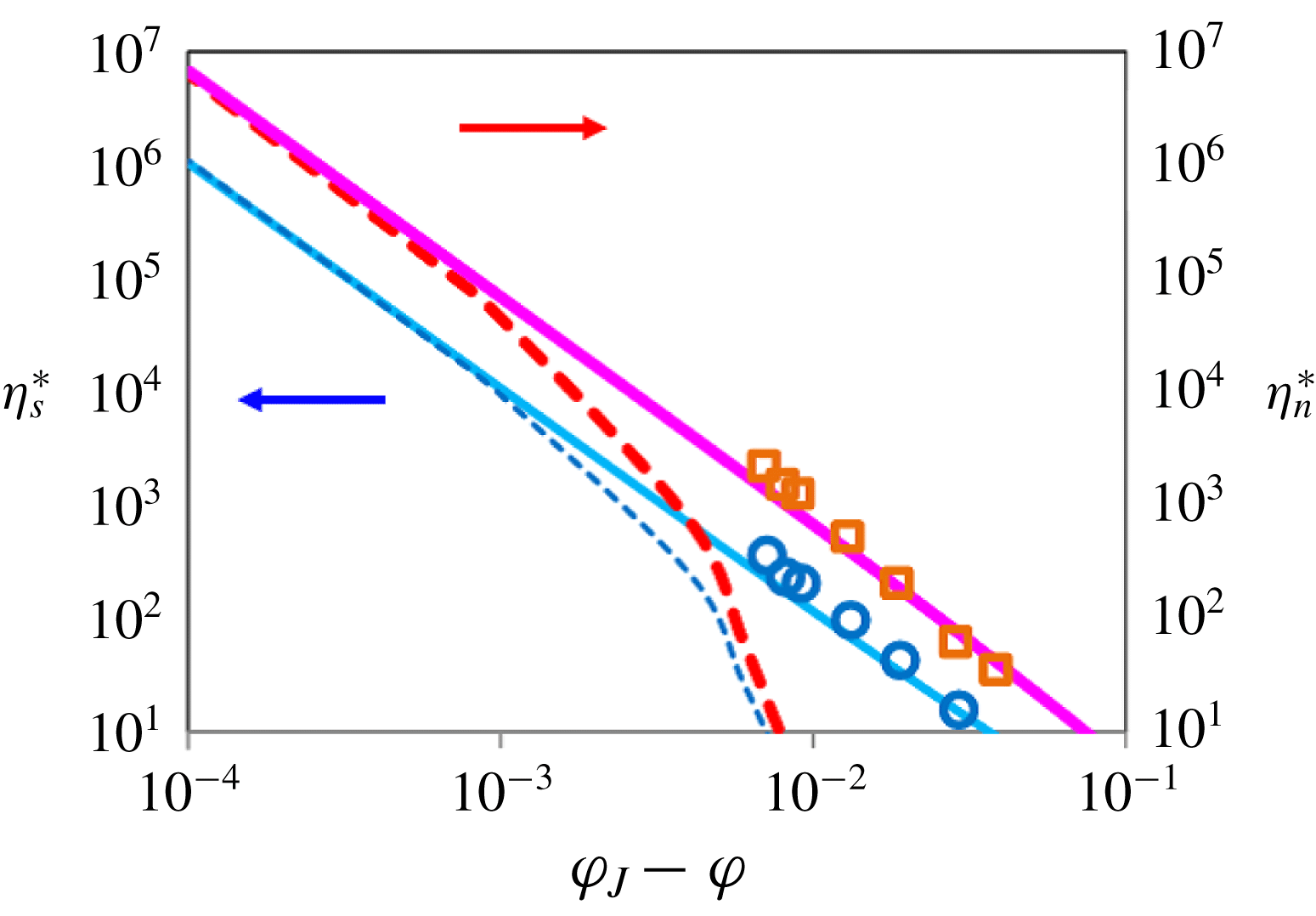
Figure 11. Shear and pressure viscosities for the case
 $\unicode[STIX]{x1D6EC}=0.04$
. The thick-solid line, thick-dashed line, open squares are the results of the pressure viscosity with splitting, without splitting and of MD. The thin-solid line, thin-dashed line, open circles are the results of the shear viscosity with splitting, without splitting and of MD.
$\unicode[STIX]{x1D6EC}=0.04$
. The thick-solid line, thick-dashed line, open squares are the results of the pressure viscosity with splitting, without splitting and of MD. The thin-solid line, thin-dashed line, open circles are the results of the shear viscosity with splitting, without splitting and of MD.
Appendix E. Comparison with empirical relations
We compare our theory with empirical relations which describe experimental results well. The empirical equations for the normalized pressure and shear viscosities are, respectively, given by
 $$\begin{eqnarray}\displaystyle & \displaystyle \unicode[STIX]{x1D702}_{n}^{\ast (MB)}=K_{n}\left(\frac{\unicode[STIX]{x1D711}/\unicode[STIX]{x1D711}_{J}}{1-\unicode[STIX]{x1D711}/\unicode[STIX]{x1D711}_{J}}\right)^{2}, & \displaystyle\end{eqnarray}$$
 $$\begin{eqnarray}\displaystyle & \displaystyle \unicode[STIX]{x1D702}_{s}^{\ast (MB)}=K_{s}\left(\frac{\unicode[STIX]{x1D711}/\unicode[STIX]{x1D711}_{J}}{1-\unicode[STIX]{x1D711}/\unicode[STIX]{x1D711}_{J}}\right)^{2}+2.5\left(\frac{\unicode[STIX]{x1D711}_{J}}{1-\unicode[STIX]{x1D711}/\unicode[STIX]{x1D711}_{J}}\right)+1, & \displaystyle\end{eqnarray}$$
where the upper script (MB) is named after the authors, and the coefficients are given by
 $K_{n}=0.75$
and
$K_{n}=0.75$
and
 $K_{s}=0.1$
(Morris & Boulay Reference Morris and Boulay1999). In figure 12, we present the results of (E 1) and (E 2), together with our theoretical results. For comparison, the results of (E 1) and (E 2) are multiplied by 0.3 for comparison. In the dense region, where the first term on the right-hand side of (E 2) is dominant, we obtain
$K_{s}=0.1$
(Morris & Boulay Reference Morris and Boulay1999). In figure 12, we present the results of (E 1) and (E 2), together with our theoretical results. For comparison, the results of (E 1) and (E 2) are multiplied by 0.3 for comparison. In the dense region, where the first term on the right-hand side of (E 2) is dominant, we obtain
 $$\begin{eqnarray}\displaystyle \unicode[STIX]{x1D707}^{(MB)}(\unicode[STIX]{x1D6FF}\unicode[STIX]{x1D711}\rightarrow 0)=\frac{\unicode[STIX]{x1D702}_{s}^{\ast (MB)}(\unicode[STIX]{x1D6FF}\unicode[STIX]{x1D711}\rightarrow 0)}{\unicode[STIX]{x1D702}_{n}^{\ast (MB)}(\unicode[STIX]{x1D6FF}\unicode[STIX]{x1D711}\rightarrow 0)}=\frac{K_{s}}{K_{n}}=0.133. & & \displaystyle\end{eqnarray}$$
This is in a relatively good agreement with the result of the present theory, 0.163. For lower densities, from (E 1) and (E 2), we obtain
 $$\begin{eqnarray}\displaystyle \unicode[STIX]{x1D707}^{(MB)}=\frac{\unicode[STIX]{x1D702}_{s}^{\ast (MB)}}{\unicode[STIX]{x1D702}_{n}^{\ast (MB)}}=\frac{K_{s}}{K_{n}}+\frac{2.5}{K_{n}(\unicode[STIX]{x1D711}/\unicode[STIX]{x1D711}_{J})^{2}}\unicode[STIX]{x1D6FF}\unicode[STIX]{x1D711}+\frac{1}{K_{n}\unicode[STIX]{x1D711}^{2}}\unicode[STIX]{x1D6FF}\unicode[STIX]{x1D711}^{2}\approx 0.133+\frac{3.33}{(\unicode[STIX]{x1D711}/\unicode[STIX]{x1D711}_{J})^{2}}\unicode[STIX]{x1D6FF}\unicode[STIX]{x1D711}, & & \displaystyle\end{eqnarray}$$
where we have neglected the
 $O(\unicode[STIX]{x1D6FF}\unicode[STIX]{x1D711}^{2})$
term in the last equality. Specifically, for
$O(\unicode[STIX]{x1D6FF}\unicode[STIX]{x1D711}^{2})$
term in the last equality. Specifically, for
 $10^{-2}<\unicode[STIX]{x1D6FF}\unicode[STIX]{x1D711}<10^{-1}$
and
$10^{-2}<\unicode[STIX]{x1D6FF}\unicode[STIX]{x1D711}<10^{-1}$
and
 $\unicode[STIX]{x1D711}_{J}=0.639$
, we obtain
$\unicode[STIX]{x1D711}_{J}=0.639$
, we obtain
 $$\begin{eqnarray}\displaystyle 0.133+3.44\unicode[STIX]{x1D6FF}\unicode[STIX]{x1D711}<\unicode[STIX]{x1D707}^{(MB)}<0.133+4.68\unicode[STIX]{x1D6FF}\unicode[STIX]{x1D711}. & & \displaystyle\end{eqnarray}$$
This is also in a relatively good agreement with our theory,
 $\unicode[STIX]{x1D707}\approx 0.163+1.78\unicode[STIX]{x1D711}^{\ast -1}\unicode[STIX]{x1D6FF}\unicode[STIX]{x1D711}$
(cf. (4.45)).
$\unicode[STIX]{x1D707}\approx 0.163+1.78\unicode[STIX]{x1D711}^{\ast -1}\unicode[STIX]{x1D6FF}\unicode[STIX]{x1D711}$
(cf. (4.45)).

Figure 12. Comparison with the empirical relation (Morris & Boulay Reference Morris and Boulay1999). The results of the normalized shear and pressure viscosities are shown in thin-dashed line and thick-dashed line, respectively. The results are multiplied by 0.3 for comparison to the theoretical results for
 $\unicode[STIX]{x1D6EC}=0.04$
shown in figure 3, which are also displayed.
$\unicode[STIX]{x1D6EC}=0.04$
shown in figure 3, which are also displayed.
Appendix F. Details of the event-driven MD simulation
The scheme of the event-driven MD simulation is discussed. It is based on the scheme for Brownian hard spheres (Scala et al. Reference Scala, Voigtmann and Michele2007), which solves the overdamped equation of motion,
 $$\begin{eqnarray}\displaystyle \unicode[STIX]{x1D701}\dot{\boldsymbol{r}}_{i}=\boldsymbol{F}_{i}^{(p)}+\unicode[STIX]{x1D701}\dot{\unicode[STIX]{x1D6FE}}y_{i}\boldsymbol{e}_{x}+\boldsymbol{F}_{i}^{(r)}. & & \displaystyle\end{eqnarray}$$
Here,
 $\unicode[STIX]{x1D701}=3\unicode[STIX]{x03C0}d\,\unicode[STIX]{x1D702}_{0}$
is the scalar resistance and
$\unicode[STIX]{x1D701}=3\unicode[STIX]{x03C0}d\,\unicode[STIX]{x1D702}_{0}$
is the scalar resistance and
 $\boldsymbol{F}_{i}^{(r)}$
is the random fluctuation force exerted by the solvent, which is assumed to be Gaussian,
$\boldsymbol{F}_{i}^{(r)}$
is the random fluctuation force exerted by the solvent, which is assumed to be Gaussian,
 $$\begin{eqnarray}\displaystyle \langle \boldsymbol{F}_{i}^{(r)}(t)\boldsymbol{F}_{i}^{(r)}(t^{\prime })\rangle =2D_{0}\unicode[STIX]{x1D701}^{2}\unicode[STIX]{x1D6FF}(t-t^{\prime }). & & \displaystyle\end{eqnarray}$$
The diffusion constant is related to
 $\unicode[STIX]{x1D701}$
as
$\unicode[STIX]{x1D701}$
as
 $D_{0}=T_{eq}/\unicode[STIX]{x1D701}$
via the fluctuation-dissipation theorem, where
$D_{0}=T_{eq}/\unicode[STIX]{x1D701}$
via the fluctuation-dissipation theorem, where
 $T_{eq}$
is the equilibrium temperature of the solvent. The units of length and time are chosen as
$T_{eq}$
is the equilibrium temperature of the solvent. The units of length and time are chosen as
 $d$
and
$d$
and
 $d^{2}/D_{0}$
. If we require that the physical mass of the particle
$d^{2}/D_{0}$
. If we require that the physical mass of the particle
 $m$
does not appear explicitly in the overdamped dynamics of (F 1), the only combination with the dimension of mass is
$m$
does not appear explicitly in the overdamped dynamics of (F 1), the only combination with the dimension of mass is
 $\unicode[STIX]{x1D701}d^{2}/D_{0}$
, and hence we choose this as the unit of mass. The algorithm consists of three steps:
$\unicode[STIX]{x1D701}d^{2}/D_{0}$
, and hence we choose this as the unit of mass. The algorithm consists of three steps:
(i) for each time step
$t_{n}=n\unicode[STIX]{x0394}t$
(
$n=0,1,\ldots$
), random velocities
$\boldsymbol{v}_{i}^{(r)}=(\unicode[STIX]{x0394}\boldsymbol{r}_{i}-\langle \unicode[STIX]{x0394}\boldsymbol{r}\rangle )/\unicode[STIX]{x0394}t$
are sampled for
$i=1,\ldots ,N$
according to the Maxwellian distribution
$f(\boldsymbol{v})=(m_{v}/(2\unicode[STIX]{x03C0}T_{eq}))^{-3/2}\exp (-m_{v}\boldsymbol{v}^{2}/(2T_{eq}))$
, where
$m_{v}$
is the ‘virtual mass’ related to
$D_{0}$
as
$D_{0}=T_{eq}\unicode[STIX]{x0394}t/(2m_{v})$
;(ii) add uniform shear velocity
$\dot{\unicode[STIX]{x1D6FE}}y_{i}\boldsymbol{e}_{x}$
to the random velocity;(iii) evolve between
$t_{n}$
and
$t_{n+1}$
by the event-driven MD.


Note that
 $m_{v}$
is a virtual quantity introduced in the Maxwellian distribution, so as to ensure the diffusive motion of the particles. In fact, from
$m_{v}$
is a virtual quantity introduced in the Maxwellian distribution, so as to ensure the diffusive motion of the particles. In fact, from
 $D_{0}=T_{eq}/\unicode[STIX]{x1D701}$
and
$D_{0}=T_{eq}/\unicode[STIX]{x1D701}$
and
 $D_{0}=T_{eq}\unicode[STIX]{x0394}t/(2m_{v})$
,
$D_{0}=T_{eq}\unicode[STIX]{x0394}t/(2m_{v})$
,
 $m_{v}$
is determined as
$m_{v}$
is determined as
 $$\begin{eqnarray}\displaystyle m_{v}=\unicode[STIX]{x1D701}\unicode[STIX]{x0394}t/2=\unicode[STIX]{x1D701}d^{2}\unicode[STIX]{x0394}t^{\ast }/(2D_{0}), & & \displaystyle\end{eqnarray}$$
which depends on
 $\unicode[STIX]{x0394}t=\unicode[STIX]{x0394}t^{\ast }d^{2}/D_{0}$
and hence is not physical. (We attach
$\unicode[STIX]{x0394}t=\unicode[STIX]{x0394}t^{\ast }d^{2}/D_{0}$
and hence is not physical. (We attach
 $\ast$
to dimensionless quantities.)
$\ast$
to dimensionless quantities.)
We modify the above scheme to adapt to non-Brownian hard spheres. We can eliminate the Brownian motion by taking the limit
 $D_{0}\rightarrow 0$
, or
$D_{0}\rightarrow 0$
, or
 $T_{eq}\rightarrow 0$
, with
$T_{eq}\rightarrow 0$
, with
 $m_{v}=\unicode[STIX]{x1D701}\unicode[STIX]{x0394}t/2$
fixed. By this choice, for each time step
$m_{v}=\unicode[STIX]{x1D701}\unicode[STIX]{x0394}t/2$
fixed. By this choice, for each time step
 $t_{n}=n\unicode[STIX]{x0394}t$
, the velocity of the particles is set to the uniform shear velocity
$t_{n}=n\unicode[STIX]{x0394}t$
, the velocity of the particles is set to the uniform shear velocity
 $\dot{\unicode[STIX]{x1D6FE}}y_{i}\boldsymbol{e}_{x}$
, and the dynamics is evolved between
$\dot{\unicode[STIX]{x1D6FE}}y_{i}\boldsymbol{e}_{x}$
, and the dynamics is evolved between
 $t_{n}$
and
$t_{n}$
and
 $t_{n+1}$
by the event-driven MD. However, taking the limit
$t_{n+1}$
by the event-driven MD. However, taking the limit
 $D_{0}\rightarrow 0$
requires us to choose other units for the time and mass, which are uniquely determined to be
$D_{0}\rightarrow 0$
requires us to choose other units for the time and mass, which are uniquely determined to be
 $\dot{\unicode[STIX]{x1D6FE}}^{-1}$
and
$\dot{\unicode[STIX]{x1D6FE}}^{-1}$
and
 $\unicode[STIX]{x1D701}/\dot{\unicode[STIX]{x1D6FE}}$
, respectively. This implies that
$\unicode[STIX]{x1D701}/\dot{\unicode[STIX]{x1D6FE}}$
, respectively. This implies that
 $\unicode[STIX]{x0394}t$
and
$\unicode[STIX]{x0394}t$
and
 $m_{v}$
should be scaled as
$m_{v}$
should be scaled as
 $$\begin{eqnarray}\displaystyle \unicode[STIX]{x0394}t=\dot{\unicode[STIX]{x1D6FE}}^{-1}\unicode[STIX]{x0394}t^{\ast } & & \displaystyle\end{eqnarray}$$
and
 $$\begin{eqnarray}\displaystyle m_{v}=(\unicode[STIX]{x1D701}/\dot{\unicode[STIX]{x1D6FE}})(\unicode[STIX]{x0394}t^{\ast }/2). & & \displaystyle\end{eqnarray}$$
Although the physical mass
 $m$
exists in real suspensions, the overdamped approximation, equation (F 1), superficially replaces
$m$
exists in real suspensions, the overdamped approximation, equation (F 1), superficially replaces
 $m$
with the virtual mass
$m$
with the virtual mass
 $m_{v}$
, which is given by (F 3) for the Brownian and (F 5) for the non-Brownian suspensions, respectively.
$m_{v}$
, which is given by (F 3) for the Brownian and (F 5) for the non-Brownian suspensions, respectively.
After equilibration from an initial configuration without overlapping of the spheres, we start the sampling. The average of the stress tensor is evaluated by
 $$\begin{eqnarray}\displaystyle \unicode[STIX]{x1D70E}_{\unicode[STIX]{x1D6FC}\unicode[STIX]{x1D6FD}}=\unicode[STIX]{x1D70E}_{\unicode[STIX]{x1D6FC}\unicode[STIX]{x1D6FD}}^{(K)}+\unicode[STIX]{x1D70E}_{\unicode[STIX]{x1D6FC}\unicode[STIX]{x1D6FD}}^{(C)}, & & \displaystyle\end{eqnarray}$$
where
 $$\begin{eqnarray}\displaystyle \unicode[STIX]{x1D70E}_{\unicode[STIX]{x1D6FC}\unicode[STIX]{x1D6FD}}^{(K)}=-\frac{1}{V}\left\langle \mathop{\sum }_{i=1}^{N}\frac{1}{m_{v}}p_{i,\unicode[STIX]{x1D6FC}}p_{i,\unicode[STIX]{x1D6FD}}\right\rangle =-\frac{1}{V}\left\langle \mathop{\sum }_{i=1}^{N}m_{v}v_{i,\unicode[STIX]{x1D6FC}}v_{i,\unicode[STIX]{x1D6FD}}\right\rangle & & \displaystyle\end{eqnarray}$$
is the average kinetic stress and
 $$\begin{eqnarray}\displaystyle \unicode[STIX]{x1D70E}_{\unicode[STIX]{x1D6FC}\unicode[STIX]{x1D6FD}}^{(C)}=-\frac{1}{V}\left\langle \mathop{\sum }_{i=1}^{N}\frac{1}{2t_{m}}\mathop{\sum }_{coll}r_{ij,\unicode[STIX]{x1D6FC}}p_{ij,\unicode[STIX]{x1D6FD}}\right\rangle =-\frac{1}{V}\left\langle \mathop{\sum }_{i=1}^{N}\frac{m_{v}}{2t_{m}}\mathop{\sum }_{coll}r_{ij,\unicode[STIX]{x1D6FC}}v_{ij,\unicode[STIX]{x1D6FD}}\right\rangle & & \displaystyle\end{eqnarray}$$
is the average contact stress, with
 $$\begin{eqnarray}\displaystyle \boldsymbol{p}_{i}=m_{v}\boldsymbol{v}_{i}=m_{v}(\dot{\boldsymbol{r}}_{i}-\dot{\unicode[STIX]{x1D6FE}}y_{i}\boldsymbol{e}_{x}) & & \displaystyle\end{eqnarray}$$
the peculiar momentum. In (F 8),
 $t_{m}$
is a time interval which is introduced to evaluate the force from the momentum transfer as
$t_{m}$
is a time interval which is introduced to evaluate the force from the momentum transfer as
 $\boldsymbol{F}_{ij}=\boldsymbol{p}_{ij}/t_{m}$
, and the summation
$\boldsymbol{F}_{ij}=\boldsymbol{p}_{ij}/t_{m}$
, and the summation
 $\sum _{coll}$
is performed over all the colliding pairs (
$\sum _{coll}$
is performed over all the colliding pairs (
 $i$
,
$i$
,
 $j$
). The parameters are set as
$j$
). The parameters are set as
 $N=1000$
,
$N=1000$
,
 $\unicode[STIX]{x0394}t^{\ast }=0.001$
and
$\unicode[STIX]{x0394}t^{\ast }=0.001$
and
 $t_{m}^{\ast }=10\unicode[STIX]{x0394}t^{\ast }=0.01$
. By the choice
$t_{m}^{\ast }=10\unicode[STIX]{x0394}t^{\ast }=0.01$
. By the choice
 $t_{m}^{\ast }\propto \unicode[STIX]{x0394}t^{\ast }$
, equation (F 8) is insensitive to
$t_{m}^{\ast }\propto \unicode[STIX]{x0394}t^{\ast }$
, equation (F 8) is insensitive to
 $\unicode[STIX]{x0394}t^{\ast }$
. Furthermore, we have verified that
$\unicode[STIX]{x0394}t^{\ast }$
. Furthermore, we have verified that
 $\unicode[STIX]{x1D70E}_{\unicode[STIX]{x1D6FC}\unicode[STIX]{x1D6FD}}^{(C)}$
is insensitive to the choice of
$\unicode[STIX]{x1D70E}_{\unicode[STIX]{x1D6FC}\unicode[STIX]{x1D6FD}}^{(C)}$
is insensitive to the choice of
 $t_{m}^{\ast }$
. We have confirmed that the results are almost insensitive to the shear rate, which exemplifies the Newtonian behaviour (cf. figure 13). We have also confirmed that, although the magnitude of
$t_{m}^{\ast }$
. We have confirmed that the results are almost insensitive to the shear rate, which exemplifies the Newtonian behaviour (cf. figure 13). We have also confirmed that, although the magnitude of
 $\unicode[STIX]{x1D70E}_{\unicode[STIX]{x1D6FC}\unicode[STIX]{x1D6FD}}^{(K)}$
is proportional to
$\unicode[STIX]{x1D70E}_{\unicode[STIX]{x1D6FC}\unicode[STIX]{x1D6FD}}^{(K)}$
is proportional to
 $\unicode[STIX]{x0394}t^{\ast }$
, it does not exhibit any divergence in approaching the jamming point, which validates (2.8). We have compared the result of the event-driven MD simulation with that of soft-sphere MD simulation (
$\unicode[STIX]{x0394}t^{\ast }$
, it does not exhibit any divergence in approaching the jamming point, which validates (2.8). We have compared the result of the event-driven MD simulation with that of soft-sphere MD simulation (
 $\dot{\unicode[STIX]{x1D6FE}}^{\ast }=10^{-7}$
) and found reasonable agreement between them (cf. figure 14).
$\dot{\unicode[STIX]{x1D6FE}}^{\ast }=10^{-7}$
) and found reasonable agreement between them (cf. figure 14).

Figure 13. (a) Shear-rate dependence of the shear viscosity and (b) the pressure viscosity. The results for
 $\unicode[STIX]{x1D711}=0.50$
, 0.60, 0.63 are shown in open diamonds, squares and triangles, respectively.
$\unicode[STIX]{x1D711}=0.50$
, 0.60, 0.63 are shown in open diamonds, squares and triangles, respectively.

Figure 14. Comparison of the theoretical result with those of hard-sphere and soft-sphere MD simulations. The results of the theory, hard-sphere MD and soft-sphere MD are shown in solid line, open diamonds and crosses, respectively.
Appendix G. Implication of the symmetry
Here we discuss another implication of the symmetry. From (2.1), the velocity distribution of the particles deviates from the uniform profile of that of the solvent,
 $\dot{\unicode[STIX]{x1D6FE}}y_{i}\boldsymbol{e}_{x}$
, if the average force is non-vanishing,
$\dot{\unicode[STIX]{x1D6FE}}y_{i}\boldsymbol{e}_{x}$
, if the average force is non-vanishing,
 $\langle \boldsymbol{F}_{i}^{(p)}\rangle \neq 0$
. However, this is actually not the case. From (3.15) and (4.9), we have
$\langle \boldsymbol{F}_{i}^{(p)}\rangle \neq 0$
. However, this is actually not the case. From (3.15) and (4.9), we have
 $$\begin{eqnarray}\displaystyle \langle \boldsymbol{F}_{i}^{(p)}\rangle & = & \displaystyle \mathop{\sum }_{j\neq i}\langle \boldsymbol{F}_{ij}^{(p)}\rangle =-\frac{1}{2}\unicode[STIX]{x1D701}_{e}\dot{\unicode[STIX]{x1D6FE}}d^{2}\mathop{\sum }_{j\neq i}\langle \hat{\boldsymbol{r}}_{ij}\unicode[STIX]{x1D6FF}(r_{ij}-d)\hat{x}_{ij}{\hat{y}}_{ij}\unicode[STIX]{x1D6E9}(-\hat{x}_{ij}{\hat{y}}_{ij})\rangle \nonumber\\ \displaystyle & = & \displaystyle -\frac{1}{2}\unicode[STIX]{x1D701}_{e}\dot{\unicode[STIX]{x1D6FE}}d^{2}\mathop{\sum }_{j\neq i}\left\{\langle \unicode[STIX]{x1D6E5}_{ij}\hat{\boldsymbol{r}}_{ij}\hat{x}_{ij}{\hat{y}}_{ij}\unicode[STIX]{x1D6E9}_{ij}\rangle _{eq}+\frac{V}{2T}\unicode[STIX]{x1D6F1}_{\unicode[STIX]{x1D6FC}\unicode[STIX]{x1D6FD}}\langle \unicode[STIX]{x1D6E5}_{ij}\hat{\boldsymbol{r}}_{ij}\hat{x}_{ij}{\hat{y}}_{ij}\unicode[STIX]{x1D6E9}_{ij}\tilde{\unicode[STIX]{x1D70E}}_{\unicode[STIX]{x1D6FC}\unicode[STIX]{x1D6FD}}\rangle _{eq}\right\},\end{eqnarray}$$
where
 $\unicode[STIX]{x1D6E5}_{ij}:=\unicode[STIX]{x1D6FF}(r_{ij}-d)$
and
$\unicode[STIX]{x1D6E5}_{ij}:=\unicode[STIX]{x1D6FF}(r_{ij}-d)$
and
 $\unicode[STIX]{x1D6E9}_{ij}:=\unicode[STIX]{x1D6E9}(-\hat{x}_{ij}{\hat{y}}_{ij})$
. From (4.25) it is obvious that the first canonical term vanishes (cubic in
$\unicode[STIX]{x1D6E9}_{ij}:=\unicode[STIX]{x1D6E9}(-\hat{x}_{ij}{\hat{y}}_{ij})$
. From (4.25) it is obvious that the first canonical term vanishes (cubic in
 $\hat{\boldsymbol{r}}_{ij}$
). By noting that
$\hat{\boldsymbol{r}}_{ij}$
). By noting that
 $\tilde{\unicode[STIX]{x1D70E}}_{\unicode[STIX]{x1D6FC}\unicode[STIX]{x1D6FD}}$
is quartic in
$\tilde{\unicode[STIX]{x1D70E}}_{\unicode[STIX]{x1D6FC}\unicode[STIX]{x1D6FD}}$
is quartic in
 $\hat{\boldsymbol{r}}$
, the second non-canonical term also vanishes. Hence, the linear profile of the velocity of the particles is preserved in the steady state.
$\hat{\boldsymbol{r}}$
, the second non-canonical term also vanishes. Hence, the linear profile of the velocity of the particles is preserved in the steady state.

Figure 15. Spherical coordinate for the angular integral.

Figure 16. Possible configurations for the double angular integrals.
Appendix H. Angular integrals
We collect the results of the angular integrals
 ${\mathcal{A}}_{pqr;stu}$
and
${\mathcal{A}}_{pqr;stu}$
and
 ${\mathcal{B}}_{pqr}$
, defined in (C 4) and (C 5). Let us introduce the following spherical coordinate (cf. figure 15),
${\mathcal{B}}_{pqr}$
, defined in (C 4) and (C 5). Let us introduce the following spherical coordinate (cf. figure 15),
 $$\begin{eqnarray}\displaystyle & \displaystyle \hat{z}=\sin \unicode[STIX]{x1D703}\cos \unicode[STIX]{x1D719}, & \displaystyle\end{eqnarray}$$
 $$\begin{eqnarray}\displaystyle & \displaystyle \hat{x}=\sin \unicode[STIX]{x1D703}\sin \unicode[STIX]{x1D719}, & \displaystyle\end{eqnarray}$$
 $$\begin{eqnarray}\displaystyle & \displaystyle {\hat{y}}=\cos \unicode[STIX]{x1D703}. & \displaystyle\end{eqnarray}$$
Then, equation (C 5) is parametrized as
 $$\begin{eqnarray}\displaystyle {\mathcal{B}}_{pqr} & = & \displaystyle \int \text{d}{\mathcal{S}}(\unicode[STIX]{x1D6E9}({\hat{y}})\unicode[STIX]{x1D6E9}(-\hat{x})+\unicode[STIX]{x1D6E9}(-{\hat{y}})\unicode[STIX]{x1D6E9}(\hat{x}))\hat{x}^{p}{\hat{y}}^{q}\hat{z}^{r}\nonumber\\ \displaystyle & = & \displaystyle \left\{\int _{0}^{1}\text{d}(\cos \unicode[STIX]{x1D703})\int _{-\unicode[STIX]{x03C0}}^{0}\text{d}\unicode[STIX]{x1D719}+\int _{-1}^{0}\text{d}(\cos \unicode[STIX]{x1D703})\int _{0}^{\unicode[STIX]{x03C0}}\text{d}\unicode[STIX]{x1D719}\right\}\hat{x}^{p}{\hat{y}}^{q}\hat{z}^{r}.\end{eqnarray}$$
Equation (C 4) is a double angular integral with respect to
 $\hat{\boldsymbol{r}}$
and
$\hat{\boldsymbol{r}}$
and
 $\hat{\boldsymbol{r}}^{\prime }$
, which can be classified into the two cases depicted in figure 16. Accordingly, it is parametrized as follows,
$\hat{\boldsymbol{r}}^{\prime }$
, which can be classified into the two cases depicted in figure 16. Accordingly, it is parametrized as follows,
 $$\begin{eqnarray}\displaystyle {\mathcal{A}}_{pqr;stu} & = & \displaystyle \left\{\int _{0}^{1}\text{d}(\cos \unicode[STIX]{x1D703})\int _{-\unicode[STIX]{x03C0}}^{0}\text{d}\unicode[STIX]{x1D719}\int _{-1}^{0}\text{d}(\cos \unicode[STIX]{x1D703}^{\prime })\int _{0}^{\unicode[STIX]{x03C0}}\text{d}\unicode[STIX]{x1D719}^{\prime }\right.\nonumber\\ \displaystyle & & \displaystyle +\left.\int _{-1}^{0}\text{d}(\cos \unicode[STIX]{x1D703})\int _{0}^{\unicode[STIX]{x03C0}}\text{d}\unicode[STIX]{x1D719}\int _{0}^{1}\text{d}(\cos \unicode[STIX]{x1D703}^{\prime })\int _{-\unicode[STIX]{x03C0}}^{0}\text{d}\unicode[STIX]{x1D719}^{\prime }\right\}\nonumber\\ \displaystyle & & \displaystyle \times \,\hat{x}^{p}{\hat{y}}^{q}\hat{z}^{r}\hat{x}^{\prime s}{\hat{y}}^{\prime t}\hat{z}^{\prime u}.\end{eqnarray}$$
Note that only the integrands which are even with respect to the parity transformation ‘
 $\hat{x}\rightarrow -\hat{x}$
and
$\hat{x}\rightarrow -\hat{x}$
and
 ${\hat{y}}\rightarrow -{\hat{y}}$
’ survive (cf. (4.22)). For parity-even terms, equation (H 5) reduces to
${\hat{y}}\rightarrow -{\hat{y}}$
’ survive (cf. (4.22)). For parity-even terms, equation (H 5) reduces to
 $$\begin{eqnarray}\displaystyle {\mathcal{A}}_{pqr;stu}=2\int _{0}^{1}\text{d}(\cos \unicode[STIX]{x1D703})\int _{-\unicode[STIX]{x03C0}}^{0}\text{d}\unicode[STIX]{x1D719}\int _{-1}^{0}\text{d}(\cos \unicode[STIX]{x1D703}^{\prime })\int _{0}^{\unicode[STIX]{x03C0}}\text{d}\unicode[STIX]{x1D719}^{\prime }\hat{x}^{p}{\hat{y}}^{q}\hat{z}^{r}\hat{x}^{\prime s}{\hat{y}}^{\prime t}\hat{z}^{\prime u}. & & \displaystyle\end{eqnarray}$$
Hence, equation (C 4) is expressed as
 $$\begin{eqnarray}\displaystyle & \displaystyle {\mathcal{A}}_{pqr;stu}=2{\mathcal{B}}_{pqr}{\mathcal{C}}_{stu}, & \displaystyle\end{eqnarray}$$
 $$\begin{eqnarray}\displaystyle & \displaystyle {\mathcal{B}}_{pqr}=\int _{0}^{1}\text{d}(\cos \unicode[STIX]{x1D703})\int _{-\unicode[STIX]{x03C0}}^{0}\text{d}\unicode[STIX]{x1D719}\,\hat{x}^{p}{\hat{y}}^{q}\hat{z}^{r}=\int _{0}^{1}\text{d}(\cos \unicode[STIX]{x1D703})\int _{-\unicode[STIX]{x03C0}}^{0}\text{d}\unicode[STIX]{x1D719}\,\cos ^{q}\unicode[STIX]{x1D703}\sin ^{p+r}\unicode[STIX]{x1D703}\sin ^{p}\unicode[STIX]{x1D719}\cos ^{r}\unicode[STIX]{x1D719}, & \displaystyle \nonumber\\ \displaystyle & & \displaystyle\end{eqnarray}$$
 $$\begin{eqnarray}\displaystyle & \displaystyle {\mathcal{C}}_{stu}=\int _{-1}^{0}\text{d}(\cos \unicode[STIX]{x1D703}^{\prime })\int _{0}^{\unicode[STIX]{x03C0}}\text{d}\unicode[STIX]{x1D719}^{\prime }\hat{x}^{\prime s}{\hat{y}}^{\prime t}\hat{z}^{\prime u}=\int _{-1}^{0}\text{d}(\cos \unicode[STIX]{x1D703}^{\prime })\int _{0}^{\unicode[STIX]{x03C0}}\text{d}\unicode[STIX]{x1D719}^{\prime }\cos ^{t}\unicode[STIX]{x1D703}\sin ^{s+u}\unicode[STIX]{x1D703}\sin ^{s}\unicode[STIX]{x1D719}\cos ^{u}\unicode[STIX]{x1D719}. & \displaystyle \nonumber\\ \displaystyle & & \displaystyle\end{eqnarray}$$
Furthermore,
 ${\mathcal{B}}_{pqr}={\mathcal{C}}_{pqr}$
holds, so we finally obtain
${\mathcal{B}}_{pqr}={\mathcal{C}}_{pqr}$
holds, so we finally obtain
 $$\begin{eqnarray}\displaystyle {\mathcal{A}}_{pqr;stu}=2{\mathcal{B}}_{pqr}{\mathcal{B}}_{stu}. & & \displaystyle\end{eqnarray}$$
It should be noted that
 ${\mathcal{B}}_{pqr}={\mathcal{B}}_{qpr}$
holds from symmetry. We collect the results of
${\mathcal{B}}_{pqr}={\mathcal{B}}_{qpr}$
holds from symmetry. We collect the results of
 ${\mathcal{B}}_{pqr}$
necessary for our purpose below:
${\mathcal{B}}_{pqr}$
necessary for our purpose below:
 $$\begin{eqnarray}\displaystyle & \displaystyle {\mathcal{B}}_{730}={\mathcal{B}}_{370}=\int _{0}^{1}\text{d}(\cos \unicode[STIX]{x1D703})\int _{-\unicode[STIX]{x03C0}}^{0}\text{d}\unicode[STIX]{x1D719}\,\cos ^{3}\unicode[STIX]{x1D703}\sin ^{7}\unicode[STIX]{x1D703}\sin ^{7}\unicode[STIX]{x1D719}=-{\textstyle \frac{64}{3465}}, & \displaystyle\end{eqnarray}$$
 $$\begin{eqnarray}\displaystyle & \displaystyle {\mathcal{B}}_{710}={\mathcal{B}}_{170}=\int _{0}^{1}\text{d}(\cos \unicode[STIX]{x1D703})\int _{-\unicode[STIX]{x03C0}}^{0}\text{d}\unicode[STIX]{x1D719}\,\cos \unicode[STIX]{x1D703}\sin ^{7}\unicode[STIX]{x1D703}\sin ^{7}\unicode[STIX]{x1D719}=-{\textstyle \frac{32}{315}}, & \displaystyle\end{eqnarray}$$
 $$\begin{eqnarray}\displaystyle & \displaystyle {\mathcal{B}}_{640}={\mathcal{B}}_{460}=\int _{0}^{1}\text{d}(\cos \unicode[STIX]{x1D703})\int _{-\unicode[STIX]{x03C0}}^{0}\text{d}\unicode[STIX]{x1D719}\,\cos ^{4}\unicode[STIX]{x1D703}\sin ^{6}\unicode[STIX]{x1D703}\sin ^{6}\unicode[STIX]{x1D719}=\frac{\unicode[STIX]{x03C0}}{231}, & \displaystyle\end{eqnarray}$$
 $$\begin{eqnarray}\displaystyle & \displaystyle {\mathcal{B}}_{620}={\mathcal{B}}_{260}=\int _{0}^{1}\text{d}(\cos \unicode[STIX]{x1D703})\int _{-\unicode[STIX]{x03C0}}^{0}\text{d}\unicode[STIX]{x1D719}\,\cos ^{2}\unicode[STIX]{x1D703}\sin ^{6}\unicode[STIX]{x1D703}\sin ^{6}\unicode[STIX]{x1D719}=\frac{\unicode[STIX]{x03C0}}{63}, & \displaystyle\end{eqnarray}$$
 $$\begin{eqnarray}\displaystyle & \displaystyle {\mathcal{B}}_{550}=\int _{0}^{1}\text{d}(\cos \unicode[STIX]{x1D703})\int _{-\unicode[STIX]{x03C0}}^{0}\text{d}\unicode[STIX]{x1D719}\,\cos ^{5}\unicode[STIX]{x1D703}\sin ^{5}\unicode[STIX]{x1D703}\sin ^{5}\unicode[STIX]{x1D719}=-{\textstyle \frac{128}{10395}}, & \displaystyle\end{eqnarray}$$
 $$\begin{eqnarray}\displaystyle & \displaystyle {\mathcal{B}}_{530}={\mathcal{B}}_{350}=\int _{0}^{1}\text{d}(\cos \unicode[STIX]{x1D703})\int _{-\unicode[STIX]{x03C0}}^{0}\text{d}\unicode[STIX]{x1D719}\,\cos ^{3}\unicode[STIX]{x1D703}\sin ^{5}\unicode[STIX]{x1D703}\sin ^{5}\unicode[STIX]{x1D719}=-{\textstyle \frac{32}{945}}, & \displaystyle\end{eqnarray}$$
 $$\begin{eqnarray}\displaystyle & \displaystyle {\mathcal{B}}_{510}={\mathcal{B}}_{150}=\int _{0}^{1}\text{d}(\cos \unicode[STIX]{x1D703})\int _{-\unicode[STIX]{x03C0}}^{0}\text{d}\unicode[STIX]{x1D719}\,\cos \unicode[STIX]{x1D703}\sin ^{5}\unicode[STIX]{x1D703}\sin ^{5}\unicode[STIX]{x1D719}=-{\textstyle \frac{16}{105}}, & \displaystyle\end{eqnarray}$$
 $$\begin{eqnarray}\displaystyle & \displaystyle {\mathcal{B}}_{440}=\int _{0}^{1}\text{d}(\cos \unicode[STIX]{x1D703})\int _{-\unicode[STIX]{x03C0}}^{0}\text{d}\unicode[STIX]{x1D719}\cos ^{4}\unicode[STIX]{x1D703}\sin ^{4}\unicode[STIX]{x1D703}\sin ^{4}\unicode[STIX]{x1D719}=\frac{\unicode[STIX]{x03C0}}{105}, & \displaystyle\end{eqnarray}$$
 $$\begin{eqnarray}\displaystyle & \displaystyle {\mathcal{B}}_{420}={\mathcal{B}}_{240}=\int _{0}^{1}\text{d}(\cos \unicode[STIX]{x1D703})\int _{-\unicode[STIX]{x03C0}}^{0}\text{d}\unicode[STIX]{x1D719}\,\cos ^{2}\unicode[STIX]{x1D703}\sin ^{4}\unicode[STIX]{x1D703}\sin ^{4}\unicode[STIX]{x1D719}=\frac{\unicode[STIX]{x03C0}}{35}, & \displaystyle\end{eqnarray}$$
 $$\begin{eqnarray}\displaystyle & \displaystyle {\mathcal{B}}_{330}=\int _{0}^{1}\text{d}(\cos \unicode[STIX]{x1D703})\int _{-\unicode[STIX]{x03C0}}^{0}\text{d}\unicode[STIX]{x1D719}\,\cos ^{3}\unicode[STIX]{x1D703}\sin ^{3}\unicode[STIX]{x1D703}\sin ^{3}\unicode[STIX]{x1D719}=-{\textstyle \frac{8}{105}}, & \displaystyle\end{eqnarray}$$
 $$\begin{eqnarray}\displaystyle & \displaystyle {\mathcal{B}}_{310}={\mathcal{B}}_{130}=\int _{0}^{1}\text{d}(\cos \unicode[STIX]{x1D703})\int _{-\unicode[STIX]{x03C0}}^{0}\text{d}\unicode[STIX]{x1D719}\,\cos \unicode[STIX]{x1D703}\sin ^{3}\unicode[STIX]{x1D703}\sin ^{3}\unicode[STIX]{x1D719}=-{\textstyle \frac{4}{15}}, & \displaystyle\end{eqnarray}$$
 $$\begin{eqnarray}\displaystyle & \displaystyle {\mathcal{B}}_{220}=\int _{0}^{1}\text{d}(\cos \unicode[STIX]{x1D703})\int _{-\unicode[STIX]{x03C0}}^{0}\text{d}\unicode[STIX]{x1D719}\,\cos ^{2}\unicode[STIX]{x1D703}\sin ^{2}\unicode[STIX]{x1D703}\sin ^{2}\unicode[STIX]{x1D719}=\frac{\unicode[STIX]{x03C0}}{15}, & \displaystyle\end{eqnarray}$$
 $$\begin{eqnarray}\displaystyle & \displaystyle {\mathcal{B}}_{040}=\int _{0}^{1}\text{d}(\cos \unicode[STIX]{x1D703})\int _{-\unicode[STIX]{x03C0}}^{0}\text{d}\unicode[STIX]{x1D719}\,\cos ^{4}\unicode[STIX]{x1D703}=\frac{\unicode[STIX]{x03C0}}{5}, & \displaystyle\end{eqnarray}$$
 $$\begin{eqnarray}\displaystyle & \displaystyle {\mathcal{B}}_{020}=\int _{0}^{1}\text{d}(\cos \unicode[STIX]{x1D703})\int _{-\unicode[STIX]{x03C0}}^{0}\text{d}\unicode[STIX]{x1D719}\,\cos ^{2}\unicode[STIX]{x1D703}=\frac{\unicode[STIX]{x03C0}}{3}, & \displaystyle\end{eqnarray}$$
 $$\begin{eqnarray}\displaystyle & \displaystyle {\mathcal{B}}_{442}=\int _{0}^{1}\text{d}(\cos \unicode[STIX]{x1D703})\int _{-\unicode[STIX]{x03C0}}^{0}\text{d}\unicode[STIX]{x1D719}\,\cos ^{4}\unicode[STIX]{x1D703}\sin ^{6}\unicode[STIX]{x1D703}\sin ^{4}\unicode[STIX]{x1D719}\cos ^{2}\unicode[STIX]{x1D719}=\frac{\unicode[STIX]{x03C0}}{1155}, & \displaystyle\end{eqnarray}$$
 $$\begin{eqnarray}\displaystyle & \displaystyle {\mathcal{B}}_{242}={\mathcal{B}}_{422}=\int _{0}^{1}\text{d}(\cos \unicode[STIX]{x1D703})\int _{-\unicode[STIX]{x03C0}}^{0}\text{d}\unicode[STIX]{x1D719}\,\cos ^{4}\unicode[STIX]{x1D703}\sin ^{4}\unicode[STIX]{x1D703}\sin ^{2}\unicode[STIX]{x1D719}\cos ^{2}\unicode[STIX]{x1D719}=\frac{\unicode[STIX]{x03C0}}{315}, & \displaystyle\end{eqnarray}$$
 $$\begin{eqnarray}\displaystyle & \displaystyle {\mathcal{B}}_{532}={\mathcal{B}}_{352}=\int _{0}^{1}\text{d}(\cos \unicode[STIX]{x1D703})\int _{-\unicode[STIX]{x03C0}}^{0}\text{d}\unicode[STIX]{x1D719}\,\cos ^{3}\unicode[STIX]{x1D703}\sin ^{7}\unicode[STIX]{x1D703}\sin ^{5}\unicode[STIX]{x1D719}\cos ^{2}\unicode[STIX]{x1D719}=-{\textstyle \frac{32}{10395}}, & \displaystyle\end{eqnarray}$$
 $$\begin{eqnarray}\displaystyle & \displaystyle {\mathcal{B}}_{152}={\mathcal{B}}_{512}=\int _{0}^{1}\text{d}(\cos \unicode[STIX]{x1D703})\int _{-\unicode[STIX]{x03C0}}^{0}\text{d}\unicode[STIX]{x1D719}\,\cos ^{5}\unicode[STIX]{x1D703}\sin ^{3}\unicode[STIX]{x1D703}\sin \unicode[STIX]{x1D719}\cos ^{2}\unicode[STIX]{x1D719}=-{\textstyle \frac{16}{945}}, & \displaystyle\end{eqnarray}$$
 $$\begin{eqnarray}\displaystyle & \displaystyle {\mathcal{B}}_{332}=\int _{0}^{1}\text{d}(\cos \unicode[STIX]{x1D703})\int _{-\unicode[STIX]{x03C0}}^{0}\text{d}\unicode[STIX]{x1D719}\,\cos ^{3}\unicode[STIX]{x1D703}\sin ^{5}\unicode[STIX]{x1D703}\sin ^{3}\unicode[STIX]{x1D719}\cos ^{2}\unicode[STIX]{x1D719}=-{\textstyle \frac{8}{945}}, & \displaystyle\end{eqnarray}$$
 $$\begin{eqnarray}\displaystyle & \displaystyle {\mathcal{B}}_{132}={\mathcal{B}}_{312}=\int _{0}^{1}\text{d}(\cos \unicode[STIX]{x1D703})\int _{-\unicode[STIX]{x03C0}}^{0}\text{d}\unicode[STIX]{x1D719}\,\cos ^{3}\unicode[STIX]{x1D703}\sin ^{3}\unicode[STIX]{x1D703}\sin \unicode[STIX]{x1D719}\cos ^{2}\unicode[STIX]{x1D719}=-{\textstyle \frac{4}{105}}, & \displaystyle\end{eqnarray}$$
 $$\begin{eqnarray}\displaystyle & \displaystyle {\mathcal{B}}_{222}=\int _{0}^{1}\text{d}(\cos \unicode[STIX]{x1D703})\int _{-\unicode[STIX]{x03C0}}^{0}\text{d}\unicode[STIX]{x1D719}\,\cos ^{2}\unicode[STIX]{x1D703}\sin ^{4}\unicode[STIX]{x1D703}\cos ^{2}\unicode[STIX]{x1D719}\sin ^{2}\unicode[STIX]{x1D719}=\frac{\unicode[STIX]{x03C0}}{105}, & \displaystyle\end{eqnarray}$$
 $$\begin{eqnarray}\displaystyle & \displaystyle {\mathcal{B}}_{112}=\int _{0}^{1}\text{d}(\cos \unicode[STIX]{x1D703})\int _{-\unicode[STIX]{x03C0}}^{0}\text{d}\unicode[STIX]{x1D719}\,\cos \unicode[STIX]{x1D703}\sin ^{3}\unicode[STIX]{x1D703}\sin \unicode[STIX]{x1D719}\cos ^{2}\unicode[STIX]{x1D719}=-{\textstyle \frac{2}{15}}. & \displaystyle\end{eqnarray}$$
In the above calculation, we have utilized the following formulas:
 $$\begin{eqnarray}\displaystyle & \displaystyle \int _{0}^{1}\text{d}(\cos \unicode[STIX]{x1D703})\cos ^{n}\unicode[STIX]{x1D703}\sin ^{m}\unicode[STIX]{x1D703}=\left\{\begin{array}{@{}c@{}}\displaystyle \int _{0}^{1}\text{d}xx^{n}(1-x^{2})^{m/2}\quad (n,m:\text{even})\\ \displaystyle \int _{0}^{\unicode[STIX]{x03C0}/2}\text{d}\unicode[STIX]{x1D703}\cos ^{n}\unicode[STIX]{x1D703}(1-\cos ^{2}\unicode[STIX]{x1D703})^{(m+1)/2}\quad (n,m:\text{odd}),\end{array}\right. & \displaystyle\end{eqnarray}$$
 $$\begin{eqnarray}\displaystyle & \displaystyle \int _{-\unicode[STIX]{x03C0}}^{0}\text{d}\unicode[STIX]{x1D719}\sin ^{n}\unicode[STIX]{x1D719}=\left\{\begin{array}{@{}c@{}}\displaystyle 2\cdot \frac{\unicode[STIX]{x03C0}}{2}\frac{(n-1)!!}{n!!}\quad (n:\text{even})\\ \displaystyle -2\cdot \frac{(n-1)!!}{n!!}\quad (n:\text{odd}).\end{array}\right. & \displaystyle\end{eqnarray}$$
From the above results for
 ${\mathcal{B}}_{pqr}$
, we obtain
${\mathcal{B}}_{pqr}$
, we obtain
 ${\mathcal{A}}_{pqr;stu}$
via (H 10) as follows,
${\mathcal{A}}_{pqr;stu}$
via (H 10) as follows,
 $$\begin{eqnarray}\displaystyle & \displaystyle {\mathcal{A}}_{420;220}={\mathcal{A}}_{240;220}=2\frac{\unicode[STIX]{x03C0}}{35}\frac{\unicode[STIX]{x03C0}}{15}=\frac{2\unicode[STIX]{x03C0}^{2}}{525}, & \displaystyle\end{eqnarray}$$
 $$\begin{eqnarray}\displaystyle & \displaystyle {\mathcal{A}}_{420;130}={\mathcal{A}}_{240;310}=2\frac{\unicode[STIX]{x03C0}}{35}\left(-\frac{4}{15}\right)=-\frac{8\unicode[STIX]{x03C0}}{525}, & \displaystyle\end{eqnarray}$$
 $$\begin{eqnarray}\displaystyle & \displaystyle {\mathcal{A}}_{330;310}={\mathcal{A}}_{330;130}=-2{\textstyle \frac{8}{105}}(-{\textstyle \frac{4}{15}})={\textstyle \frac{64}{1575}}, & \displaystyle\end{eqnarray}$$
 $$\begin{eqnarray}\displaystyle & \displaystyle {\mathcal{A}}_{330;220}=-2\frac{8}{105}\frac{\unicode[STIX]{x03C0}}{15}=-\frac{16\unicode[STIX]{x03C0}}{1575}, & \displaystyle\end{eqnarray}$$
 $$\begin{eqnarray}\displaystyle & \displaystyle {\mathcal{A}}_{310;130}={\mathcal{A}}_{130;130}=2(-{\textstyle \frac{4}{15}})^{2}={\textstyle \frac{32}{225}}, & \displaystyle\end{eqnarray}$$
 $$\begin{eqnarray}\displaystyle & \displaystyle {\mathcal{A}}_{310;220}={\mathcal{A}}_{130;220}=2\left(-\frac{4}{15}\right)\frac{\unicode[STIX]{x03C0}}{15}=-\frac{8\unicode[STIX]{x03C0}}{225}, & \displaystyle\end{eqnarray}$$
 $$\begin{eqnarray}\displaystyle & \displaystyle {\mathcal{A}}_{310;112}={\mathcal{A}}_{130;112}=2(-{\textstyle \frac{4}{15}})(-{\textstyle \frac{2}{15}})={\textstyle \frac{16}{225}}, & \displaystyle\end{eqnarray}$$
 $$\begin{eqnarray}\displaystyle & \displaystyle {\mathcal{A}}_{220;220}=2\left(\frac{\unicode[STIX]{x03C0}}{15}\right)^{2}=\frac{2\unicode[STIX]{x03C0}^{2}}{225}, & \displaystyle\end{eqnarray}$$
 $$\begin{eqnarray}\displaystyle & \displaystyle {\mathcal{A}}_{220;112}=2\frac{\unicode[STIX]{x03C0}}{15}\left(-\frac{2}{15}\right)=-\frac{4\unicode[STIX]{x03C0}}{225}, & \displaystyle\end{eqnarray}$$
 $$\begin{eqnarray}\displaystyle & \displaystyle {\mathcal{A}}_{222;112}=2\frac{\unicode[STIX]{x03C0}}{105}\left(-\frac{2}{15}\right)=-\frac{4\unicode[STIX]{x03C0}}{1575}, & \displaystyle\end{eqnarray}$$
 $$\begin{eqnarray}\displaystyle & \displaystyle {\mathcal{A}}_{040;310}={\mathcal{A}}_{040;130}=2\frac{\unicode[STIX]{x03C0}}{5}\left(-\frac{4}{15}\right)=-\frac{8\unicode[STIX]{x03C0}}{75}, & \displaystyle\end{eqnarray}$$
 $$\begin{eqnarray}\displaystyle & \displaystyle {\mathcal{A}}_{040;220}=2\frac{\unicode[STIX]{x03C0}}{5}\frac{\unicode[STIX]{x03C0}}{15}=\frac{2\unicode[STIX]{x03C0}^{2}}{75}, & \displaystyle\end{eqnarray}$$
 $$\begin{eqnarray}\displaystyle & \displaystyle {\mathcal{A}}_{040;112}=2\frac{\unicode[STIX]{x03C0}}{5}\left(-\frac{2}{15}\right)=-\frac{4\unicode[STIX]{x03C0}}{75}, & \displaystyle\end{eqnarray}$$
 $$\begin{eqnarray}\displaystyle & \displaystyle {\mathcal{A}}_{020;310}={\mathcal{A}}_{020;130}=2\frac{\unicode[STIX]{x03C0}}{3}\left(-\frac{4}{15}\right)=-\frac{8\unicode[STIX]{x03C0}}{45}, & \displaystyle\end{eqnarray}$$
 $$\begin{eqnarray}\displaystyle & \displaystyle {\mathcal{A}}_{020;220}=2\frac{\unicode[STIX]{x03C0}}{3}\frac{\unicode[STIX]{x03C0}}{15}=\frac{2\unicode[STIX]{x03C0}^{2}}{45}, & \displaystyle\end{eqnarray}$$
 $$\begin{eqnarray}\displaystyle & \displaystyle {\mathcal{A}}_{020;112}=2\frac{\unicode[STIX]{x03C0}}{3}\left(-\frac{2}{15}\right)=-\frac{4\unicode[STIX]{x03C0}}{45}, & \displaystyle\end{eqnarray}$$
 $$\begin{eqnarray}\displaystyle & \displaystyle {\mathcal{A}}_{510;220}={\mathcal{A}}_{150;220}=-2\frac{16}{105}\frac{\unicode[STIX]{x03C0}}{15}=-\frac{32\unicode[STIX]{x03C0}}{1575}, & \displaystyle\end{eqnarray}$$
 $$\begin{eqnarray}\displaystyle & \displaystyle {\mathcal{A}}_{510;130}={\mathcal{A}}_{150;130}=-2{\textstyle \frac{16}{105}}(-{\textstyle \frac{4}{15}})={\textstyle \frac{128}{1575}}. & \displaystyle\end{eqnarray}$$
Appendix I. Four-point susceptibility
The simulation method for the four-point susceptibility is shown. The four-point density correlation function is given by
 $$\begin{eqnarray}\displaystyle g^{(4)}(\boldsymbol{r}_{1},\boldsymbol{r}_{2},t)=\langle \unicode[STIX]{x1D70C}(\boldsymbol{r}_{1},0)\unicode[STIX]{x1D70C}(\boldsymbol{r}_{1},t)\unicode[STIX]{x1D70C}(\boldsymbol{r}_{2},0)\unicode[STIX]{x1D70C}(\boldsymbol{r}_{2},t)\rangle -\langle \unicode[STIX]{x1D70C}(\boldsymbol{r}_{1},0)\unicode[STIX]{x1D70C}(\boldsymbol{r}_{1},t)\rangle \langle \unicode[STIX]{x1D70C}(\boldsymbol{r}_{2},0)\unicode[STIX]{x1D70C}(\boldsymbol{r}_{2},t)\rangle , & & \displaystyle \nonumber\\ \displaystyle & & \displaystyle\end{eqnarray}$$
where
 $\unicode[STIX]{x1D70C}(\boldsymbol{r},t):=\sum _{i=1}^{N}\unicode[STIX]{x1D6FF}(\boldsymbol{r}-\boldsymbol{r}_{i}(t))$
is the density. The four-point susceptibility is obtained by integrating the spatial degrees of freedom in
$\unicode[STIX]{x1D70C}(\boldsymbol{r},t):=\sum _{i=1}^{N}\unicode[STIX]{x1D6FF}(\boldsymbol{r}-\boldsymbol{r}_{i}(t))$
is the density. The four-point susceptibility is obtained by integrating the spatial degrees of freedom in
 $g^{(4)}(\boldsymbol{r}_{1},\boldsymbol{r}_{2},t)$
,
$g^{(4)}(\boldsymbol{r}_{1},\boldsymbol{r}_{2},t)$
,
 $$\begin{eqnarray}\displaystyle \unicode[STIX]{x1D712}_{4}^{0}(t)=\frac{\unicode[STIX]{x1D6FD}V}{N^{2}}\int \text{d}^{3}\boldsymbol{r}_{1}\int \text{d}^{3}\boldsymbol{r}_{2}\,g^{(4)}(\boldsymbol{r}_{1},\boldsymbol{r}_{2},t), & & \displaystyle\end{eqnarray}$$
where
 $\unicode[STIX]{x1D6FD}$
is the inverse temperature. This can be expressed by the order parameter
$\unicode[STIX]{x1D6FD}$
is the inverse temperature. This can be expressed by the order parameter
 $$\begin{eqnarray}\displaystyle Q_{0}(t):=\int \text{d}^{3}\boldsymbol{r}\unicode[STIX]{x1D70C}(\boldsymbol{r},0)\unicode[STIX]{x1D70C}(\boldsymbol{r},t)=\mathop{\sum }_{i=1}^{N}\mathop{\sum }_{j=1}^{N}\unicode[STIX]{x1D6FF}(\boldsymbol{r}_{i}(0)-\boldsymbol{r}_{j}(t)) & & \displaystyle\end{eqnarray}$$
as
 $$\begin{eqnarray}\displaystyle \unicode[STIX]{x1D712}_{4}^{0}(t)=\frac{\unicode[STIX]{x1D6FD}V}{N^{2}}[\langle Q_{0}(t)^{2}\rangle -\langle Q_{0}(t)\rangle ^{2}]. & & \displaystyle\end{eqnarray}$$
There is a problem in evaluating
 $\unicode[STIX]{x1D712}_{4}^{0}(t)$
by a simulation, because
$\unicode[STIX]{x1D712}_{4}^{0}(t)$
by a simulation, because
 $Q_{0}(t)$
is ill defined for a finite system. We follow the method of Glotzer, Novikov & Schröder (Reference Glotzer, Novikov and Schröder2000) and modify
$Q_{0}(t)$
is ill defined for a finite system. We follow the method of Glotzer, Novikov & Schröder (Reference Glotzer, Novikov and Schröder2000) and modify
 $Q_{0}(t)$
by an ‘overlap’ function
$Q_{0}(t)$
by an ‘overlap’ function
 $w(r)$
(Parisi Reference Parisi1997) that is unity inside a region of size
$w(r)$
(Parisi Reference Parisi1997) that is unity inside a region of size
 $a$
and zero otherwise, where
$a$
and zero otherwise, where
 $a$
is chosen to be of the order of the particle diameter:
$a$
is chosen to be of the order of the particle diameter:
 $$\begin{eqnarray}\displaystyle Q(t) & := & \displaystyle \int \text{d}^{3}\boldsymbol{r}_{1}\int \text{d}^{3}\boldsymbol{r}_{2}\unicode[STIX]{x1D70C}(\boldsymbol{r}_{1},0)\unicode[STIX]{x1D70C}(\boldsymbol{r}_{2},t)w(|\boldsymbol{r}_{1}-\boldsymbol{r}_{2}|)\nonumber\\ \displaystyle & = & \displaystyle \mathop{\sum }_{i=1}^{N}\mathop{\sum }_{j=1}^{N}\int \text{d}^{3}\boldsymbol{r}w(|\boldsymbol{r}|)\unicode[STIX]{x1D6FF}(\boldsymbol{r}+\boldsymbol{r}_{i}(0)-\boldsymbol{r}_{j}(t))=\mathop{\sum }_{i=1}^{N}\mathop{\sum }_{j=1}^{N}w(|\boldsymbol{r}_{ij}-\unicode[STIX]{x1D741}_{j}|).\end{eqnarray}$$
Here
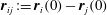 $\boldsymbol{r}_{ij}:=\boldsymbol{r}_{i}(0)-\boldsymbol{r}_{j}(0)$
,
$\boldsymbol{r}_{ij}:=\boldsymbol{r}_{i}(0)-\boldsymbol{r}_{j}(0)$
,
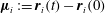 $\unicode[STIX]{x1D741}_{i}:=\boldsymbol{r}_{i}(t)-\boldsymbol{r}_{i}(0)$
and
$\unicode[STIX]{x1D741}_{i}:=\boldsymbol{r}_{i}(t)-\boldsymbol{r}_{i}(0)$
and
 $a$
is chosen as
$a$
is chosen as
 $0.3\,d$
. Replacing
$0.3\,d$
. Replacing
 $Q_{0}(t)$
by
$Q_{0}(t)$
by
 $Q(t)$
yields
$Q(t)$
yields
 $$\begin{eqnarray}\displaystyle \unicode[STIX]{x1D712}_{4}(t)=\frac{\unicode[STIX]{x1D6FD}V}{N^{2}}[\langle Q(t)^{2}\rangle -\langle Q(t)\rangle ^{2}], & & \displaystyle\end{eqnarray}$$
which we have measured by MD simulation (cf. figure 9).


