


1. Introduction
The classic (uniform) random recursive tree is a natural stochastic growth model, which has been proposed for numerous applications in such areas as chain letters [Reference Gastwirth and Bhattacharya9] and philology [Reference Najock and Heyde14]. These trees grow according to a uniform attachment scheme in which each existing node has an equal chance of recruiting a new entrant. For a detailed discussion of properties, see [Reference Drmota7], [Reference Frieze and KaroŃski8], and [Reference Smythe and Mahmoud16].
Certain applications have encouraged new paths of research. It was observed that uniform attachment does not capture particular clustering features in real-world networks and does not give rise to the power laws and scale-free behavior that are characteristic of real applications. Real-world networks have features described by the Matthew principle, according to which ‘the rich get richer’ or ‘success breeds success’. Many of these features are generated by a degree-preferential attachment model, in which fat nodes of higher degree are given preference at recruiting new entrants. More precisely, a node recruits according to a probability proportional to its outdegree [Reference Smythe, Mahmoud and SzymaŃski17]. The model introduced by BarabÁsi and Albert in [Reference BarabÁsi and Albert3] and discussed in [Reference Albert and BarabÁsi1] is slightly different, where the recruiting is done with probability proportional to one plus the outdegree. The same BarabÁsi–Albert scheme was rigorously developed for the first time in [Reference BollobÁs, Riordan and Spencer4]. The random graphs in these sources are not limited to trees. For a broader discussion, see [Reference BarabÁsi2].
Until now, the term preferential attachment has been reserved for this degree-preference model. However, other applications can conceivably require us to consider an alternative preferential attachment mechanism. For example, in the bonding of atoms to form compounds, unsaturated atoms have higher affinity to other unsaturated atoms. Less saturated atoms are hungrier for bonding. This constitutes a preferential attachment scheme inversely proportional to the valence of an atom in a chemical compound.
Other preferential attachment schemes may depend on the dynamics of the tree growth. In a social network, affinity may be proportional to node age, whereby older nodes represent popularity and experience in social success. Or as an alternative model, affinity may be proportional to the youthfulness of a node, which models the eagerness of newcomers to expand their social network. Trees grown under old-age preference have been considered in the recent book [Reference Hofri and Mahmoud11]. Here we consider preferential attachment dominated by youth.
2. Young-age attachment trees
We study a random tree model that assumes that younger nodes have stronger affinity. This assumption is appropriate for networks in which new entrants tend to recruit more members. For example, frequently clubs offer new members a special deal – possibly discount memberships – that they can share with friends for a specified time. Or in the case of modeling disease transmission, for diseases with varying intensity of communicability, recently infected persons will be more likely to infect others.
In this model, a recursive tree grows in the following fashion. The tree starts at time 0 with one node; let us label it 1. At each subsequent point  $t\ge 1$
in discrete time, one of the nodes in the existing tree attracts (recruits) the nth (
$t\ge 1$
in discrete time, one of the nodes in the existing tree attracts (recruits) the nth ( $(t+1$
)st) entrant in the system, and a node labeled n is attached to the recruiter, considered the parent. Thus
$(t+1$
)st) entrant in the system, and a node labeled n is attached to the recruiter, considered the parent. Thus  $t-i+1$
is the amount of time node i spent living in the tree; we take it to be the age of node i by time t.
$t-i+1$
is the amount of time node i spent living in the tree; we take it to be the age of node i by time t.
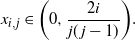
The tree grows in such a way that younger nodes have a higher probability of attracting new nodes. Concretely, the probability that the ith node  $(i=1,\ldots,n-1)$
is chosen as the parent of node n is proportional to the node index, which implies younger nodes have greater affinity. Letting
$(i=1,\ldots,n-1)$
is chosen as the parent of node n is proportional to the node index, which implies younger nodes have greater affinity. Letting  ${\mathcal A}_{i,n}$
be the event that the nth node attaches to the ith node, the proposed young-age attachment model is governed by the probability
${\mathcal A}_{i,n}$
be the event that the nth node attaches to the ith node, the proposed young-age attachment model is governed by the probability
 \begin{equation}{\mathbb P}({\mathcal A}_{i,n}) = \frac{2i}{n(n-1)} \quad \text{for } 1\le i\le n-1.\end{equation}
Figure 1 illustrates the six young-age preferential trees of size 4. The numbers in the top row are their probabilities.
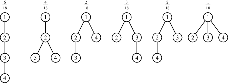
Figure 1: Young-age attachment recursive trees of size 4 and their probabilities.
3. Scope and organization
The manuscript is organized as follows. Distributional properties of the outdegree of node  $i =1, 2, \ldots, n$
are derived in Section 4. The mean and variance are established, and Poisson limit results are found via Chen–Stein Poisson approximation methods. Tree leaves are examined in Section 5, and limit results are obtained for the fraction of leaves in a given tree as the size of the tree grows. We find that the young-age probability model results in a fraction of leaves less than 1/2. Section 6 is devoted to the investigation of various properties of the insertion depth of node n, where it is found that the exact distribution involves Stirling numbers of the first kind. Upon appropriate normalization, concentration laws and Gaussian limits are established. In the concluding remarks of Section 7, the young-age model is contrasted with the uniform case and areas of potential future research are discussed.
$i =1, 2, \ldots, n$
are derived in Section 4. The mean and variance are established, and Poisson limit results are found via Chen–Stein Poisson approximation methods. Tree leaves are examined in Section 5, and limit results are obtained for the fraction of leaves in a given tree as the size of the tree grows. We find that the young-age probability model results in a fraction of leaves less than 1/2. Section 6 is devoted to the investigation of various properties of the insertion depth of node n, where it is found that the exact distribution involves Stirling numbers of the first kind. Upon appropriate normalization, concentration laws and Gaussian limits are established. In the concluding remarks of Section 7, the young-age model is contrasted with the uniform case and areas of potential future research are discussed.
4. Outdegrees
Let  $\Delta_{i,n}$
be the outdegree of node i in a young-age attachment tree of size n – a count of the children of node i right after the node n joins the tree. If we take
$\Delta_{i,n}$
be the outdegree of node i in a young-age attachment tree of size n – a count of the children of node i right after the node n joins the tree. If we take  ${\mathbb I}_{\mathcal B}$
to be the indicator of event
${\mathbb I}_{\mathcal B}$
to be the indicator of event  $\mathcal B$
, we can express the random variable
$\mathcal B$
, we can express the random variable  $\Delta_{i,n}$
as a sum of indicators for the events
$\Delta_{i,n}$
as a sum of indicators for the events  ${\mathcal A}_{i,j}$
with
${\mathcal A}_{i,j}$
with  $j \gt i$
:
$j \gt i$
:
 \begin{equation*} \Delta_{i,n} = \sum_{j=i+1}^{n}{\mathbb I}_{{\mathcal A}_{i,j}}.\end{equation*}
4.1. Exact moment generating function
The events  ${\mathcal A}_{i,j}$
are independent. Consequently, the moment generating function of
${\mathcal A}_{i,j}$
are independent. Consequently, the moment generating function of  $\Delta_{i,n}$
is the product of the individual Bernoulli moment generating functions:
$\Delta_{i,n}$
is the product of the individual Bernoulli moment generating functions:
 \begin{equation}\phi_{\Delta_{i,n}}(t) =\prod_{j=i+1}^{n} \biggl(1+\frac{2i}{j( j-1) }( {\mathrm{e}}^t-1) \biggr).\end{equation}
4.1.1. Mean and variance
Using the moment generating function, we have the expectation and variance. In the presentation, we need the nth harmonic number of the second order,  $H_n^{(2)} = \sum_{k=1}^n 1/k^2$
.
$H_n^{(2)} = \sum_{k=1}^n 1/k^2$
.
Proposition 4.1. Let  $\Delta_{i,n}$
be the outdegree of node i right after node n joins the young-age attachment tree. We have
$\Delta_{i,n}$
be the outdegree of node i right after node n joins the young-age attachment tree. We have
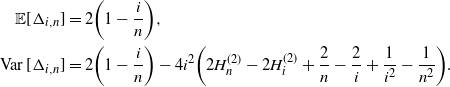 \begin{align*}{\mathbb E}[\Delta_{i,n}] &=2\biggl( 1-\frac{i}{n}\biggr),\operatorname{Var} [\Delta_{i,n}] &= 2\biggl( 1-\frac{i}{n}\biggr) -4i^2\biggl( 2 H_n^{(2)} - 2 H_i^{(2)} + \frac 2 n - \frac 2 i + \frac 1 {i^2} - \frac 1 {n^2}\biggr).\end{align*}
Proof. Take the first derivative of the moment generating function with respect to t, and evaluate it at 0 using the chain rule, to get
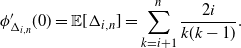 \begin{equation*}\phi_{\Delta_{i,n}}' (0) ={\mathbb E}[\Delta_{i,n}] = \sum_{k=i+1}^{n} \frac{2i}{k(k-1)}\notag . \end{equation*}
Decomposing the summand into partial fractions, the sum telescopes:
 \begin{equation}{\mathbb E}[\Delta_{i,n}] =2i\sum_{j=i+1}^{n}\biggl( \frac{1}{j-1}-\frac{1}{j}\biggr) =2i\biggl( \frac{1}{i}-\frac{1}{n}\biggr) =2\biggl( 1-\frac{i}{n}\biggr).\end{equation}
The variance of  $\Delta_{i,n}$
follows after computing the second derivative of the moment generating function evaluated at
$\Delta_{i,n}$
follows after computing the second derivative of the moment generating function evaluated at  $t=0$
. To expedite the computation, write the derivative of the moment generating function using the chain rule
$t=0$
. To expedite the computation, write the derivative of the moment generating function using the chain rule
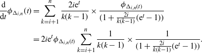 \begin{align*}\frac {\mathrm{d}} {{\mathrm{d}} t}\phi_{\Delta_{i,n}}(t) &=\sum_{k=i+1}^{n}\frac {2i {\mathrm{e}}^t} {k(k-1)} \times \frac {\phi_{\Delta_{i,n}(t)}}{(1+\tfrac{2i}{k(k-1) }( {\mathrm{e}}^t-1) )} &= 2i {\mathrm{e}}^t \phi_{\Delta_{i,n}(t)}\sum_{k=i+1}^{n}\frac 1 {k(k-1)} \times \frac 1 {(1+\tfrac{2i}{k(k-1) }( {\mathrm{e}}^t-1))} .\end{align*}
The second derivative at 0 is
 \begin{align*}\frac {{\mathrm{d}}^2} {{\mathrm{d}} t^2}\phi_{\Delta_{i,n}}(0) &= {\mathbb E}[\Delta_{i,n}^2] &= 2i ({\mathrm{e}}^t \phi_{\Delta_{i,n}}'(t) + {\mathrm{e}}^t \phi_{\Delta_{i,n}} (t))\biggl|_{t=0}\sum_{k=i+1}^{n}\frac 1 {k(k-1)} \\ &\quad\, + 2i {\mathrm{e}}^t \phi_{\Delta_{i,n}}(t)\sum_{k=i+1}^{n} \frac 1 {k(k-1)} \times \frac {-2i {\mathrm{e}}^t / (k(k-1))} {(1+\tfrac{2i}{k(k-1) }( {\mathrm{e}}^t-1))^2}\biggr|_{t=0} \\ &= 2i ({\mathbb E}[\Delta_{i,n}] + 1) \times \frac 1 {2i}\, {\mathbb E}[\Delta_{i,n}] - 4i^2 \sum_{k=i+1}^{n} \frac 1 {k^2(k-1)^2} &= {\mathbb E}^2[\Delta_{i,n}] + {\mathbb E}[\Delta_{i,n}] - 4i^2 \sum_{k=i+1}^{n} \frac 1 {k^2(k-1)^2} .\end{align*}
Using the form (4.2), we have
 \begin{align*}\operatorname{Var} [\Delta_{i,n}] & ={\mathbb E}[\Delta_{i,n}^{2}] -{\mathbb E}^2[\Delta_{i,n}] & ={\mathbb E}[\Delta_{i,n}] - 4 i^2\sum_{k=i+1}^{n} \frac 1{k^2(k-1)^2 } & =2\biggl( 1-\frac{i}{n}\biggr) - 4i^2\sum_{k=i+1}^{n} \frac 1 {k^2(k-1)^2 }.\end{align*}
The variance as stated in Proposition 4.1 follows after expanding the summand in partial fractions and recognizing the harmonic numbers in the sums.
4.1.2. Interpretation
We immediately see one way in which the behavior in young-age preferential attachment trees contrasts with the uniform attachment model. In young-age preferential attachment trees, for fixed i, the expected outdegree of node i remains small and bounded by 2, whereas in the uniform attachment tree the expected outdegree of node i (fixed) by the time node n joins is asymptotic to  $\ln n$
, and thus grows without a bound.
$\ln n$
, and thus grows without a bound.
In the young-age preferential attachment tree, we see ‘phases’ depending on the relation of i to n. For ‘small’ i, where  $i=o(n)$
, such as the case
$i=o(n)$
, such as the case  $i= 7$
or
$i= 7$
or  $i=\lceil 3 \ln n + 6\rceil$
, we have
$i=\lceil 3 \ln n + 6\rceil$
, we have  ${\mathbb E}[\Delta_{i,n}] \to 2.$
For
${\mathbb E}[\Delta_{i,n}] \to 2.$
For  $i\sim\alpha n$
with
$i\sim\alpha n$
with  $0<\alpha \le 1$
, such as the example
$0<\alpha \le 1$
, such as the example  $i = \lceil \frac{5}{7} n + 2 \sqrt n\, + 12 \ln n + \pi^2\rceil$
, we have
$i = \lceil \frac{5}{7} n + 2 \sqrt n\, + 12 \ln n + \pi^2\rceil$
, we have  ${\mathbb E}[\Delta_{i,n}] \to2(1-\alpha)$
. Note that for the very late arriving nodes, corresponding to
${\mathbb E}[\Delta_{i,n}] \to2(1-\alpha)$
. Note that for the very late arriving nodes, corresponding to  $i\sim n$
, such as the case
$i\sim n$
, such as the case  $i = \lfloor n - 7 n^{{{3}/{4}}} + \sqrt n\, \rfloor$
, we have
$i = \lfloor n - 7 n^{{{3}/{4}}} + \sqrt n\, \rfloor$
, we have  ${\mathbb E}[\Delta_{i,n}] \to 0$
.
${\mathbb E}[\Delta_{i,n}] \to 0$
.
One can notice a delicate balance. It is true that if n is large, the relative affinity of a young node with large index i is much higher than the old early nodes. However, the early nodes have stayed much longer in the tree and had repeated opportunities to recruit, particularly when they themselves were young and had high affinity. So, after all, it is not surprising that the early nodes have slightly higher expected outdegrees.
The variance  $\operatorname{Var} [\Delta_{i,n}]$
is quite close to the expected value
$\operatorname{Var} [\Delta_{i,n}]$
is quite close to the expected value  ${\mathbb E}[\Delta_{i,n}]$
. Again, we have different phases depending on the relation between i and n. There are two phases for ‘small’ i with
${\mathbb E}[\Delta_{i,n}]$
. Again, we have different phases depending on the relation between i and n. There are two phases for ‘small’ i with  $i=o(n) $
. When i is fixed, we have
$i=o(n) $
. When i is fixed, we have
 \begin{equation*}\operatorname{Var} [\Delta_{i,n}] \to 8 i + 8 i^2\biggl( \frac {\pi^2} 6 - H_i^{(2)}\biggr) - 2.\end{equation*}
When  $i=o(n) $
and
$i=o(n) $
and  $i\to\infty$
, we have
$i\to\infty$
, we have
 \begin{equation*}\operatorname{Var} [\Delta_{i,n}] \to 2. \end{equation*}
For  $i\sim\alpha n$
, with
$i\sim\alpha n$
, with  $0<\alpha \le 1$
, we get
$0<\alpha \le 1$
, we get  $\operatorname{Var} [\Delta_{i,n}] \to 2( 1-\alpha)$
. Note again that for
$\operatorname{Var} [\Delta_{i,n}] \to 2( 1-\alpha)$
. Note again that for  $i\sim n$
, we have
$i\sim n$
, we have  $\operatorname{Var} [\Delta_{i,n}] \to 0$
.
$\operatorname{Var} [\Delta_{i,n}] \to 0$
.
4.2. Limit distribution
The moment generating function (4.1) allows us to directly derive the main limit result of this section. However, we first outline some necessary background material concerning probability distance measures and Chen–Stein approximation.
4.2.1. Preliminaries
For any two random variables X and Y, respectively, with induced measures  $\mathbb P$
and
$\mathbb P$
and  $\mathbb Q$
on the real line, we define the total variation distance
$\mathbb Q$
on the real line, we define the total variation distance
 \begin{equation*}d_{\mathrm{TV}}(X,Y):=\sup_{A\in \mathcal{B}}\, \vert {\mathbb P}( A) -\mathbb Q(A) \vert, \end{equation*}
where A is an element of the Borel sigma algebra on  $\mathbb R$
.
$\mathbb R$
.
It is well known that for discrete random variables, convergence in total variation distance is equivalent to convergence in distribution.
Lemma 4.1. ([Reference Gut10]) For a sequence  $X_n$
of discrete random variables and a discrete random variable X, we have
$X_n$
of discrete random variables and a discrete random variable X, we have
 \begin{equation*} d_{\mathrm{TV}}(X_{n},X) \to 0 \iff X_n \buildrel d \over \longrightarrow X.\end{equation*}
This lays out a strategy for the proof. We aim to show that the total variation distance between  $X_n$
and a limiting random variable converges to 0, implying convergence in distribution.
$X_n$
and a limiting random variable converges to 0, implying convergence in distribution.
A useful tool is a bound on the total variation distance between Poisson random variables.
In what follows we denote a Poisson random variable with parameter θ by Poi(θ).
Lemma 4.2. If  $\nu>\mu$
and X and Y are respectively distributed like
$\nu>\mu$
and X and Y are respectively distributed like  $ {\rm Poi}(\nu)$
and
$ {\rm Poi}(\nu)$
and  ${\rm Poi}(\mu)$
, then we have
${\rm Poi}(\mu)$
, then we have
 \begin{equation*}d_{\mathrm{TV}}(X,Y) \le \nu-\mu. \end{equation*}
Proof. We use  $\,\buildrel d \over =\, $
for equality in distribution. Let
$\,\buildrel d \over =\, $
for equality in distribution. Let  $Y^{*}$
and Z be independent random variables with
$Y^{*}$
and Z be independent random variables with  $Y^{*}\, \buildrel d \over =\, {\rm Poi}(\mu)$
,
$Y^{*}\, \buildrel d \over =\, {\rm Poi}(\mu)$
,  $Z \, \buildrel d \over = \, {\rm Poi}(\nu - \mu)$
and define
$Z \, \buildrel d \over = \, {\rm Poi}(\nu - \mu)$
and define  $X^{*}=Y^{*} + Z \,\buildrel d \over =\, {\rm Poi}(\nu)$
. By [Reference Gut10, Lemma 7.1] we have
$X^{*}=Y^{*} + Z \,\buildrel d \over =\, {\rm Poi}(\nu)$
. By [Reference Gut10, Lemma 7.1] we have
 \begin{equation*} d_{\mathrm{TV}}(X^{*},Y^{*}) \le {\mathbb P}(X^{*} \ne Y^{*}) = {\mathbb P} (Z \neq 0) = 1 -{\mathbb P}(Z=0) = 1 - {\mathrm{e}}^{-(\nu - \mu)} \le \nu - \mu.\end{equation*}
Note that  $(X^{*},Y^{*})$
is a coupling of (X,Y), so
$(X^{*},Y^{*})$
is a coupling of (X,Y), so  $d_{\mathrm{TV}}(X,Y) = d_{\mathrm{TV}}(X^{*},Y^{*}) \leq \nu - \mu$
.
$d_{\mathrm{TV}}(X,Y) = d_{\mathrm{TV}}(X^{*},Y^{*}) \leq \nu - \mu$
.
The main Chen–Stein result we use applies to approximating sums of independent Bernoulli random variables with a Poisson random variable [Reference Ross15].
Proposition 4.2. Let  $X_{1},\ldots,X_{n}$
be independent Bernoulli random variables with
$X_{1},\ldots,X_{n}$
be independent Bernoulli random variables with  ${\mathbb P}( X_{i}=1) =p_{i}$
. If
${\mathbb P}( X_{i}=1) =p_{i}$
. If  $W_n=\sum_{i=1}^{n}X_{i}$
and
$W_n=\sum_{i=1}^{n}X_{i}$
and  $\lambda_n ={\mathbb E}[W_n] = \sum_{i=1}^{n}p_{i}$
, then we have
$\lambda_n ={\mathbb E}[W_n] = \sum_{i=1}^{n}p_{i}$
, then we have
 \begin{equation*}d_{\mathrm{TV}}(W_n,{\rm Poi} ( \lambda_n)) \le \min \biggl\{ 1,\frac{1}{\lambda_n}\biggr\} \sum_{i=1}^{n}p_{i}^{2}\le \min \{ 1,\lambda_n \} \max_{1\le i \le n}p_{i}. \end{equation*}
Proof. See Theorem 4.6 of [Reference Ross15]
4.2.2. Limit laws
The index i and the age n can be tied together in many complicated ways. For instance, one might think of a bizarre sequence in which
 \begin{equation*}i = i(n) = \begin{cases} 2 & \text{if \textit{n} is even}, \\[5pt]
\lfloor \sqrt n \rfloor & \text{if \textit{n} is odd}.\end{cases}\end{equation*}
\begin{equation*}i = i(n) = \begin{cases} 2 & \text{if \textit{n} is even}, \\[5pt]
\lfloor \sqrt n \rfloor & \text{if \textit{n} is odd}.\end{cases}\end{equation*}
Such a sequence is not likely to appear in any application and does not lead to convergence. Like sequences are not within the scope of this investigation. We focus on relations between i and n with a systematic unifying theme for the growth of both. Namely, our investigation covers convergence relations that arise when  $i = i(n) = \alpha n + o(n)$
, for
$i = i(n) = \alpha n + o(n)$
, for  $\alpha \in [0, 1]$
. So i has an infinite limit, except for the case
$\alpha \in [0, 1]$
. So i has an infinite limit, except for the case  $\alpha = 0$
, where we require the o(n) term to have a non-oscillating leading term, such as, for example,
$\alpha = 0$
, where we require the o(n) term to have a non-oscillating leading term, such as, for example,  $i=7$
or
$i=7$
or  $i = \lceil 3 \ln n + 6\rceil$
.
$i = \lceil 3 \ln n + 6\rceil$
.
Theorem 4.1. As  $n\to\infty,$
 $\Delta_{i,n}$
converges in distribution. Consider a node with index
$\Delta_{i,n}$
converges in distribution. Consider a node with index  $i = i(n) = \alpha n + o(n)$
, for
$i = i(n) = \alpha n + o(n)$
, for  $0 \le \alpha\le 1$
. When
$0 \le \alpha\le 1$
. When  $\lim_{n\to \infty} i(n)$
exists, we have
$\lim_{n\to \infty} i(n)$
exists, we have
 \begin{equation*}\Delta_{i,n}\buildrel d \over \longrightarrow \Delta_{i}= {\rm Poi}(2(1-\alpha)) +Y_{\lim_{n\to \infty} i(n)},\end{equation*}
where  $Y_{\lim_{n\to \infty} i(n)}$
is a zero-mean integer-valued random variable negatively correlated with the
$Y_{\lim_{n\to \infty} i(n)}$
is a zero-mean integer-valued random variable negatively correlated with the  ${\rm Poi}(2(1-\alpha))$
component.
${\rm Poi}(2(1-\alpha))$
component.
For fixed i, with  $\alpha = 0$
, we have
$\alpha = 0$
, we have
 \begin{equation*} {\mathbb E} [ \Delta_{i} ] = 2, \end{equation*}
 \begin{equation*} \operatorname{Var} [ \Delta_{i} ] = 2 - \frac 4 3 \, \pi^2 i^2 +8 i^2 H_i^{(2)}+ 8i - 4, \end{equation*}
 \begin{equation*}0
< d_{\mathrm{TV}} (\Delta_{i}, {\rm Poi}(2)) \le \frac 2 {i+1},\end{equation*}
\begin{equation*}0
< d_{\mathrm{TV}} (\Delta_{i}, {\rm Poi}(2)) \le \frac 2 {i+1},\end{equation*}
whereas, for any growing  $i = i(n) \to \infty$
, we have
$i = i(n) \to \infty$
, we have  $Y_\infty = 0$
, almost surely.
$Y_\infty = 0$
, almost surely.
Proof. For the first statement of the theorem, we work with a logarithmic transformation of  $\phi_{\Delta_{i,n}}(t)$
:
$\phi_{\Delta_{i,n}}(t)$
:
 \begin{equation*}\ln \phi_{\Delta_{i,n}}(t) =\sum_{j=i+1}^{n}\ln\biggl(1+\frac{2i}{j( j-1) }( {\mathrm{e}}^t-1) \biggr).\end{equation*}
We seek a Taylor series expansion of  $\ln(1+x) $
around zero for each summand. To make use of the expansion, we need
$\ln(1+x) $
around zero for each summand. To make use of the expansion, we need
 \begin{equation*} -1<\frac{2i}{j( j-1) }( {\mathrm{e}}^t-1)
< 1 \quad \text{for } j\ge 1.\end{equation*}
\begin{equation*} -1<\frac{2i}{j( j-1) }( {\mathrm{e}}^t-1)
< 1 \quad \text{for } j\ge 1.\end{equation*}
These inequalities restrict the values of t for which the expansion is well-defined. The upper bounds require
 \begin{equation*}t<\ln \biggl( 1+\frac{j( j-1) }{2i}\biggr)\end{equation*}
for  $j\ge 1$
, and the upper bounds are nested as j increases. So all the inequalities will be true when
$j\ge 1$
, and the upper bounds are nested as j increases. So all the inequalities will be true when
 \begin{equation*} t<\ln \biggl( 1+\frac{( i+1) i}{2i}\biggr) =\ln \biggl( 1+\frac{i+1}{2}\biggr), \end{equation*}
and since  $i \ge 1$
, the expansion is well-defined for all i,j, when
$i \ge 1$
, the expansion is well-defined for all i,j, when  $t <\ln 2$
.
$t <\ln 2$
.
With  $1\le i<j\le n$
, for negative t the lower bound is automatically satisfied. In summary, Taylor series expansions are valid for all i and j, when
$1\le i<j\le n$
, for negative t the lower bound is automatically satisfied. In summary, Taylor series expansions are valid for all i and j, when  $t\in ( -\infty,\ln 2 )$
.
$t\in ( -\infty,\ln 2 )$
.
The next step is to show that  $\lim_{n}\phi _{\Delta_{i,n}}( t) $
is finite for all
$\lim_{n}\phi _{\Delta_{i,n}}( t) $
is finite for all  $t\in ( -\infty, \ln 2 )$
. Trivially, we have
$t\in ( -\infty, \ln 2 )$
. Trivially, we have  $\lim_{n\to\infty}\phi _{\Delta_{i,n}}(0)=1.$
Next consider
$\lim_{n\to\infty}\phi _{\Delta_{i,n}}(0)=1.$
Next consider  $t\in ( 0,\ln 2)$
. Take a first-order Taylor series expansion around zero using the remainder form and apply the expression for the mean
$t\in ( 0,\ln 2)$
. Take a first-order Taylor series expansion around zero using the remainder form and apply the expression for the mean  ${\mathbb E}[\Delta_{i,n}]$
, to get
${\mathbb E}[\Delta_{i,n}]$
, to get
 \begin{align*}\ln \phi _{\Delta_{i,n}}( t) &=\sum_{j=i+1}^{n}\frac{2i}{j(j-1) }( {\mathrm{e}}^t-1)-\frac{1}{2}\sum_{j=i+1}^{n}\biggl( \frac{1}{1+x_{i,j}}\biggr) ^{2}\biggl( \frac{2i}{j( j-1) }\, ({\mathrm{e}}^t-1) \biggr) ^{2}, &=2\biggl( 1-\frac{i}{n}\biggr) ( {\mathrm{e}}^t-1) -2i^2({\mathrm{e}}^t-1)^{2}\sum_{j=i+1}^{n}\biggl( \frac{1}{1+x_{i,j}}\biggr) ^{2} \biggl( \frac{1}{j^2(j-1)^2 }\biggr),\end{align*}
for some
 \begin{equation*}x_{i,j}\in \biggl( 0, \frac{2i}{j(j-1) }( {\mathrm{e}}^t-1) \biggr) ,\end{equation*}
for all  $j\ge 1$
.
$j\ge 1$
.
Evidently the series is convergent; let us define
 \begin{equation*} h_{\lim_{n\to\infty} i(n) } (t) = \lim_{n\to\infty} -2\sum_{j=i(n)+1}^{n}\biggl( \frac{1}{1+x_{i,j}}\biggr) ^{2}\biggl( \frac{i(n)}{j( j-1) }\,({\mathrm{e}}^t-1) \biggr) ^{2} ,\end{equation*}
and note that  $|h_{\lim_{n\to\infty} i(n) } (t) | < \infty$
.
$|h_{\lim_{n\to\infty} i(n) } (t) | < \infty$
.
Since
 \begin{equation*}2\biggl( 1-\frac{i}{n}\biggr) ( {\mathrm{e}}^t-1)\to 2(1-\alpha)( {\mathrm{e}}^t-1),\end{equation*}
we have
 \begin{equation*}\ln \phi _{\Delta_{i,n}}( t) \to 2(1-\alpha)( {\mathrm{e}}^t-1)+ h_{\lim_{n\to\infty}i(n)}(t)
< \infty.\end{equation*}
\begin{equation*}\ln \phi _{\Delta_{i,n}}( t) \to 2(1-\alpha)( {\mathrm{e}}^t-1)+ h_{\lim_{n\to\infty}i(n)}(t)
< \infty.\end{equation*}
An identical argument holds for the negative part of the interval and thus
 \begin{equation*}\phi_{\Delta_{i,n}}( t) \to {\mathrm{e}}^{2(1-\alpha)( {\mathrm{e}}^t-1)}\,{\mathrm{e}}^{h_{\lim_{n\to\infty}i(n)}(t)} \quad \text{for } t\in ( -\infty,\ln 2). \end{equation*}
As the convergence of  $\phi_{\Delta_{i,n}}( t)$
occurs over a finite open interval containing 0, by the Curtiss theorem [Reference Curtiss6], the limit function
$\phi_{\Delta_{i,n}}( t)$
occurs over a finite open interval containing 0, by the Curtiss theorem [Reference Curtiss6], the limit function  ${\mathrm{e}}^{2(1-\alpha)( {\mathrm{e}}^t-1)}\,{\mathrm{e}}^{h_{\lim_{n\to\infty}i(n)}(t)}$
is the moment generating function of some random variable, which we call
${\mathrm{e}}^{2(1-\alpha)( {\mathrm{e}}^t-1)}\,{\mathrm{e}}^{h_{\lim_{n\to\infty}i(n)}(t)}$
is the moment generating function of some random variable, which we call  $\Delta_i$
.
$\Delta_i$
.
From the structure of the limit moment generating function, the limiting random variable  $\Delta_i$
is ‘close’ to a
$\Delta_i$
is ‘close’ to a  ${\rm Poi} (2(1-\alpha))$
random variable along with a perturbation random variable
${\rm Poi} (2(1-\alpha))$
random variable along with a perturbation random variable  $Y_{\lim_{n\to\infty} i(n)}$
with moment generating function
$Y_{\lim_{n\to\infty} i(n)}$
with moment generating function  ${\mathrm{e}}^{h_{\lim_{n\to\infty}i(n)}(t)}$
.
${\mathrm{e}}^{h_{\lim_{n\to\infty}i(n)}(t)}$
.
Fixed i. Let  $P_{i,n}$
be a sequence of totally independent Poisson random variables, with
$P_{i,n}$
be a sequence of totally independent Poisson random variables, with
 \begin{equation*}P_{i,n} \buildrel d \over = {\rm Poi} \biggl(2\biggl( 1- \frac{i}{n} \biggr)\biggr).\end{equation*}
These will be the sequence of approximating random variables that we want to be ‘close’ to  $\Delta_{i,n}$
.
$\Delta_{i,n}$
.
The triangle inequality holds for the total variation distance:
 \begin{equation*}d_{\mathrm{TV}}(\Delta_{i},{\rm Poi} (2)) \le d_{\mathrm{TV}}(\Delta_{i},\Delta_{i,n} ) + d_{\mathrm{TV}} (\Delta_{i,n},{\rm Poi} (2)).\end{equation*}
Using the triangle inequality a second time, we have an inequality valid for all n, which is namely
 \begin{equation*} d_{\mathrm{TV}}(\Delta_{i},{\rm Poi} (2)) \le d_{\mathrm{TV}}(\Delta_{i},\Delta_{i,n} ) + d_{\mathrm{TV}}(\Delta_{i,n},P_{i,n}) + d_{\mathrm{TV}}(P_{i,n},{\rm Poi} (2)).\end{equation*}
We now consider each term in order. Since  $\Delta_{i,n} \buildrel d \over \longrightarrow \Delta_{i}$
, by Lemma 4.1,
$\Delta_{i,n} \buildrel d \over \longrightarrow \Delta_{i}$
, by Lemma 4.1,  $d_{\mathrm{TV}}(\Delta_{i},\Delta_{i,n} ) \to 0$
. With
$d_{\mathrm{TV}}(\Delta_{i},\Delta_{i,n} ) \to 0$
. With  $\Delta_{i,n}$
being a sum of independent indicators, Proposition 4.2 is applicable, with
$\Delta_{i,n}$
being a sum of independent indicators, Proposition 4.2 is applicable, with  $\lambda_n = 2(1-i/n)$
. From the upper inequality of Proposition 4.2, for large n we get
$\lambda_n = 2(1-i/n)$
. From the upper inequality of Proposition 4.2, for large n we get
 \begin{equation*} d_{\mathrm{TV}}(\Delta_{i,n},P_{i,n}) \le\min \biggl\{ 1,2 \biggl(1- \frac i n\biggr) \biggr\} \max_{i+1 \le j \le n} \frac {2i} {j(j-1)}= 1 \times \frac{2i}{i(i+1)}= \frac{2}{i+1}.\end{equation*}
Finally, by Lemma 4.2, we have
 \begin{equation*} d_{\mathrm{TV}}(P_{i,n},{\rm Poi} (2)) \le 2 - 2\biggl( 1-\frac{i}{n}\biggr) = \frac{2i}{n}.\end{equation*}
Taken together, as  $n \to \infty$
, we have
$n \to \infty$
, we have
 \begin{equation*} 0
< \lim_{n\to \infty} d_{\mathrm{TV}}(\Delta_{i},{\rm Poi} (2)) \le \lim_{n\to \infty} d_{\mathrm{TV}}(\Delta_{i} ,\Delta_{i,n}) + \lim_{n\to \infty} \frac{2}{i+1} + \lim_{n\to \infty} \frac {2i} n.\end{equation*}
\begin{equation*} 0
< \lim_{n\to \infty} d_{\mathrm{TV}}(\Delta_{i},{\rm Poi} (2)) \le \lim_{n\to \infty} d_{\mathrm{TV}}(\Delta_{i} ,\Delta_{i,n}) + \lim_{n\to \infty} \frac{2}{i+1} + \lim_{n\to \infty} \frac {2i} n.\end{equation*}
For fixed i, this becomes
 \begin{equation*} 0
< d_{\mathrm{TV}} (\Delta_{i},{\rm Poi} (2)) \le 0 + \lim_{n\to \infty} \frac{2}{i+1} + 0 = \frac{2}{i+1},\end{equation*}
\begin{equation*} 0
< d_{\mathrm{TV}} (\Delta_{i},{\rm Poi} (2)) \le 0 + \lim_{n\to \infty} \frac{2}{i+1} + 0 = \frac{2}{i+1},\end{equation*}
as claimed.
The mean and variance of the limiting distribution follows from uniform integrability arguments. Except in pathological cases, the limit of the individual random variable moments will pass through to the limit distribution. Furthermore, similar arguments show that the  $Y_{\lim_{i\to \infty} i(n)}$
component is negatively correlated with the Poisson piece.
$Y_{\lim_{i\to \infty} i(n)}$
component is negatively correlated with the Poisson piece.
Growing i. Consider  $i= i(n) = \alpha n + o(n)$
, with
$i= i(n) = \alpha n + o(n)$
, with  $\alpha\in (0, 1]$
. By the triangle inequality, we have
$\alpha\in (0, 1]$
. By the triangle inequality, we have
 \begin{equation*} d_{\mathrm{TV}}(\Delta_{i,n},{\rm Poi} (2(1-\alpha))) \le d_{\mathrm{TV}}(\Delta_{i,n},P_{i,n} ) + d_{\mathrm{TV}}(P_{i,n},{\rm Poi} (2(1-\alpha))).\end{equation*}
By Proposition 4.2 and Lemma 4.2, we obtain
 \begin{equation*}d_{\mathrm{TV}}(\Delta_{i,n},{\rm Poi} (2(1-\alpha))) \le \frac{2}{i+1} + 2\, \biggl| \alpha - \frac{i}{n} \biggr|.\end{equation*}
As  $n \to \infty$
, we have the convergence
$n \to \infty$
, we have the convergence  ${{2}/{(i+1)}} \to 0$
, since
${{2}/{(i+1)}} \to 0$
, since  $i\to \infty$
and
$i\to \infty$
and  $ {{i}/{n}} \to \alpha$
. So we have
$ {{i}/{n}} \to \alpha$
. So we have
 \begin{equation*}d_{\mathrm{TV}}(\Delta_{i,n},{\rm Poi} (2(1-\alpha))) \to 0.\end{equation*}
Thus we have  $\Delta_{i,n} \buildrel d \over \longrightarrow {\rm Poi} (2(1-\alpha))$
and
$\Delta_{i,n} \buildrel d \over \longrightarrow {\rm Poi} (2(1-\alpha))$
and  $Y_\infty = 0$
.
$Y_\infty = 0$
.
Remark 4.1. The limit law in Theorem 4.1 combines all the phases discussed in the interpretations in Section 4.1.2 and better explains how they merge at the ‘seam lines’. One can say that
 \begin{equation*}\Delta_{i,n} \buildrel d \over \longrightarrow {\rm Poi}(2(1-\alpha)) + Y_{\lim_{n\to\infty} i(n)}.\end{equation*}
In the very early phase (fixed i),  $\alpha = 0$
, and the role of
$\alpha = 0$
, and the role of  $Y_{\lim_{n\to\infty} i(n)} = Y_i$
is pronounced. The assertion that, for fixed i, we have
$Y_{\lim_{n\to\infty} i(n)} = Y_i$
is pronounced. The assertion that, for fixed i, we have
 \begin{equation*}0
< d_{\mathrm{TV}} (\Delta_{i}, {\rm Poi}(2)) \le \frac 2 {i+1}\end{equation*}
\begin{equation*}0
< d_{\mathrm{TV}} (\Delta_{i}, {\rm Poi}(2)) \le \frac 2 {i+1}\end{equation*}
is actually a qualifying description of the random variable  $Y_i$
.
$Y_i$
.
Then, for intermediate i, growing to infinity, but remaining o(n),  $\alpha$
is still 0, and the effect of
$\alpha$
is still 0, and the effect of  $Y_{\lim_{n\to\infty} i(n)} = Y_\infty = 0$
disappears. An instance of this case is
$Y_{\lim_{n\to\infty} i(n)} = Y_\infty = 0$
disappears. An instance of this case is  $i = \lceil 3 \ln n + 6\rceil$
.
$i = \lceil 3 \ln n + 6\rceil$
.
In the linear phase  $i \sim \alpha n$
, with
$i \sim \alpha n$
, with  $0 < \alpha < 1$
, the Poisson parameter is attenuated. An instance of this case is
$0 < \alpha < 1$
, the Poisson parameter is attenuated. An instance of this case is  $i = \lceil \frac{5}{7} n + 2 \sqrt n\, + 12 \ln n+ \pi^2\rceil.$
Ultimately the Poisson parameter becomes 0, when
$i = \lceil \frac{5}{7} n + 2 \sqrt n\, + 12 \ln n+ \pi^2\rceil.$
Ultimately the Poisson parameter becomes 0, when  $i \sim n$
. Here the limit is a
$i \sim n$
. Here the limit is a  ${\rm Poi} (0)$
random variable, which is identically 0. An instance of this case is
${\rm Poi} (0)$
random variable, which is identically 0. An instance of this case is  $i = \lfloor n - 7 n^{{{3}/{4}}} + \sqrt n\,\rfloor$
.
$i = \lfloor n - 7 n^{{{3}/{4}}} + \sqrt n\,\rfloor$
.
Remark 4.2. It is assumed in Theorem 4.1 that  $\lim_{n\to\infty} i(n)$
exists. If this limit does not exist, as in the example discussed at the beginning of this subsection, the interpretation is that
$\lim_{n\to\infty} i(n)$
exists. If this limit does not exist, as in the example discussed at the beginning of this subsection, the interpretation is that  $\Delta_{i,n}$
does not converge in distribution at all to any limit. Rather, it oscillates.
$\Delta_{i,n}$
does not converge in distribution at all to any limit. Rather, it oscillates.
5. Leaves
Let  ${\mathbb L}_{i,n}$
be an indicator equal to 1 when node i is a leaf in a tree of size n and 0 otherwise. Define
${\mathbb L}_{i,n}$
be an indicator equal to 1 when node i is a leaf in a tree of size n and 0 otherwise. Define  $L_{n}$
to be the number of leaves in a tree of size n, which can be expressed as the sum of the individual leaf indicators:
$L_{n}$
to be the number of leaves in a tree of size n, which can be expressed as the sum of the individual leaf indicators:
 \begin{equation*} L_{n}=\sum_{i=1}^{n}{\mathbb L}_{i,n}.\end{equation*}
Under the young-age attachment model, the root is never a leaf in a tree with size  $n \gt 1$
; node n is always a leaf in any size tree. Since node attachments are independent, we can directly calculate the mean and variance of the leaf indicators.
$n \gt 1$
; node n is always a leaf in any size tree. Since node attachments are independent, we can directly calculate the mean and variance of the leaf indicators.
 \begin{equation*}{\mathbb E}[ {\mathbb L}_{i,n}] = \prod_{j=i+1}^{n} \biggl( 1-\frac{2i}{j(j-1)}\biggr), \end{equation*}
and
 \begin{equation*}\operatorname{Var} [ {\mathbb L}_{i,n}] = \prod_{j=i+1}^{n} \biggl( 1-\frac{2i}{j(j-1)}\biggr) \biggl[ 1 - \prod_{j=i+1}^{n} \biggl( 1-\frac{2i}{j(j-1)}\biggr) \biggr]. \end{equation*}
Proof. For node i to be a leaf in a tree of size  $n>i$
, it must be passed over by every node
$n>i$
, it must be passed over by every node  $j>i,$
which each occurs with probability
$j>i,$
which each occurs with probability  $1-{{2i}/{(j(j-1))}}.$
These attachments are independent, whence the joint probability is the product of the individual probabilities:
$1-{{2i}/{(j(j-1))}}.$
These attachments are independent, whence the joint probability is the product of the individual probabilities:
 \begin{equation*} {\mathbb E}[ {\mathbb L}_{i,n}] = {\mathbb P}( {\mathbb L}_{i,n}=1) = \prod_{j=i+1}^{n} \biggl( 1-\frac{2i}{j(j-1)}\biggr). \end{equation*}
The variance follows immediately since the  ${\mathbb L}_{i,n}$
are Bernoulli random variables.
${\mathbb L}_{i,n}$
are Bernoulli random variables.
We have a complete characterization of the marginal distributions of the leaf indicators in a tree of size  $n > 1$
:
$n > 1$
:
 \begin{align*}{\mathbb L}_{1,n} &=0 \quad \text{with probability 1}, {\mathbb L}_{i,n} &= \text{Bernoulli}\biggl(\prod_{j=i+1}^{n} \biggl( 1-\frac{2i}{j(j-1)}\biggr) \biggr) \quad \text{for } 1 < i
< n, {\mathbb L}_{n,n} &=1 \quad \text{with probability 1}.\end{align*}
\begin{align*}{\mathbb L}_{1,n} &=0 \quad \text{with probability 1}, {\mathbb L}_{i,n} &= \text{Bernoulli}\biggl(\prod_{j=i+1}^{n} \biggl( 1-\frac{2i}{j(j-1)}\biggr) \biggr) \quad \text{for } 1 < i
< n, {\mathbb L}_{n,n} &=1 \quad \text{with probability 1}.\end{align*}
5.1. Joint distribution
While node attachments are independent, the resulting  ${\mathbb L}_{i,n}$
are dependent. Nevertheless, the structure of the leaf indicators allows us to derive useful covariance results, which we use to study the asymptotic behavior. Throughout this section we state the results in a more general form since they hold for any sequence of attachment distributions.
${\mathbb L}_{i,n}$
are dependent. Nevertheless, the structure of the leaf indicators allows us to derive useful covariance results, which we use to study the asymptotic behavior. Throughout this section we state the results in a more general form since they hold for any sequence of attachment distributions.
Recall that  ${\mathcal A}_{i,n}$
denotes the event that the nth node attaches to the ith node. Assume now that for node
${\mathcal A}_{i,n}$
denotes the event that the nth node attaches to the ith node. Assume now that for node  $n\ge2$
, we have a general attachment model:
$n\ge2$
, we have a general attachment model:
 \begin{equation*} {\mathbb P}({\mathcal A}_{i,n}) = f_{n}(i) \quad \text{for } 1\le i\le n-1,\end{equation*}
with  $f_{n}(i) \ge 0$
and
$f_{n}(i) \ge 0$
and  $\sum_{i=1}^{n-1} f_{n}(i) = 1.$
In principle this allows for arbitrary individual attachment probabilities for each node at each time of entry. We can directly calculate the cross-expectation of the  ${\mathbb L}_{i,n}$
.
${\mathbb L}_{i,n}$
.
Lemma 5.2. With  $i<j$
, we have
$i<j$
, we have
 \begin{equation*}{\mathbb E}[ {\mathbb L}_{i,n} {\mathbb L}_{j,n}] =\prod_{p=i+1}^{j} ( 1- f_{p}(i) )\prod_{p=j+1}^{n} ( 1- f_{p}(i) - f_{p}(j)).\end{equation*}
Proof. Assume without loss of generality that  $i<j$
. The product
$i<j$
. The product  ${\mathbb L}_{i,n}{\mathbb L}_{j,n}$
is equal to one when node i is passed over by the nodes
${\mathbb L}_{i,n}{\mathbb L}_{j,n}$
is equal to one when node i is passed over by the nodes  $p=i+1$
to j, and then both nodes i and j are passed over for nodes
$p=i+1$
to j, and then both nodes i and j are passed over for nodes  $p=j+1$
to n. The first sequence of events each happen with probability
$p=j+1$
to n. The first sequence of events each happen with probability  $ 1- f_{p}(i) $
and the latter sequence of events each occur with probability
$ 1- f_{p}(i) $
and the latter sequence of events each occur with probability  $ 1- f_{p}(i) - f_{p}(j) $
. All of these node attachments are independent, so the joint probability is the product of probabilities for the individual events.
$ 1- f_{p}(i) - f_{p}(j) $
. All of these node attachments are independent, so the joint probability is the product of probabilities for the individual events.
The cross-expectation allows us to find an upper bound for the covariance of the leaf indicators.
Theorem 5.1. For  $i \neq j$
, we have
$i \neq j$
, we have
 \begin{equation*} \operatorname{Cov} [{\mathbb L}_{i,n},{\mathbb L}_{j,n}] \leq 0 .\end{equation*}
Proof. The rightmost expression for the cross-expectation in Lemma 5.2 is
 \begin{equation*}\prod_{p=j+1}^{n} ( 1- f_{p}(i) - f_{p}(j)).\end{equation*}
We note for each p:
 \begin{equation*}1- f_{p}(i) - f_{p}(j) \leq 1 - f_{p}(i) - f_{p}(j) + f_{p}(i)f_{p}(j)= ( 1- f_{p}(i) ) ( 1 - f_{p}(j)).\end{equation*}
Thus we have
 \begin{equation*}\prod_{p=j+1}^{n} ( 1- f_{p}(i) - f_{p}(j)) \le \prod_{p=j+1}^{n} ( 1- f_{p}(i)) ( 1 - f_{p}(j)).\end{equation*}
Substituting this inequality into the cross-expectation of Lemma 5.2 and collecting the i and j terms, we obtain
 \begin{align*} {\mathbb E}[ {\mathbb L}_{i,n} {\mathbb L}_{j,n}]& \le \prod_{p=i+1}^{j} ( 1- f_{p}(i) )\prod_{p=j+1}^{n} ( 1- f_{p}(i) ) ( 1- f_{p}(j)) & = \prod_{p=i+1}^{n} ( 1- f_{p}(i) ) \prod_{p=j+1}^{n} ( 1- f_{p}(j) ) & = {\mathbb E}[ {\mathbb L}_{i,n}] \, {\mathbb E}[ {\mathbb L}_{j,n}],\end{align*}
which implies that the covariance is non-positive.
5.2. Mean and variance
Specifying the young-age preferential model, we use the cross-expectation in Lemma 5.2 to express the covariance between leaves with  $i<j$
.
$i<j$
.
 \begin{align*}\operatorname{Cov} [{\mathbb L}_{i,n},{\mathbb L}_{j,n}] &= \prod_{p=i+1}^{j} \biggl( 1-\frac{2i}{p(p-1)}\biggr)\prod_{p=j+1}^{n} \biggl( 1-\frac{2(i + j)}{p(p-1)}\biggr)&\quad\, - \prod_{p=i+1}^{n} \biggl( 1-\frac{2i}{p(p-1)}\biggr)\prod_{p=j+1}^{n} \biggl( 1-\frac{2j}{p(p-1)}\biggr).\end{align*}
With the expression for the expectation of  ${\mathbb L}_{i,n}$
in hand, we can calculate the mean and variance for
${\mathbb L}_{i,n}$
in hand, we can calculate the mean and variance for  $L_{n}$
, when
$L_{n}$
, when  $n>1$
:
$n>1$
:
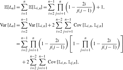 \begin{align*} {\mathbb E}[ L_{n} ] &= \sum_{i=1}^{n} {\mathbb E}[ {\mathbb L}_{i,n} ] = \sum_{i=2}^{n-1} \prod_{j=i+1}^{n} \biggl( 1-\frac{2i}{j(j-1)}\biggr) + 1, \\ \operatorname{Var} [ L_{n} ] &= \sum_{i=2}^{n-1} \operatorname{Var} [ {\mathbb L}_{i,n} ] + 2\sum_{i=2}^{n-2} \sum_{j=i+1}^{n-1}\operatorname{Cov} [{\mathbb L}_{i,n},{\mathbb L}_{j,n}] &= \sum_{i=2}^{n-1} \prod_{j=i+1}^{n} \biggl( 1-\frac{2i}{j(j-1)}\biggr) \biggl[ 1 - \prod_{j=i+1}^{n} \biggl( 1-\frac{2i}{j(j-1)}\biggr) \biggr] & \quad\, + 2\sum_{i=2}^{n-2} \sum_{j=i+1}^{n-1}\operatorname{Cov} [{\mathbb L}_{i,n},{\mathbb L}_{j,n}],\end{align*}
where  $\operatorname{Cov} [{\mathbb L}_{i,n},{\mathbb L}_{j,n}]$
is the covariance in Corollary 5.1.
$\operatorname{Cov} [{\mathbb L}_{i,n},{\mathbb L}_{j,n}]$
is the covariance in Corollary 5.1.
5.3. Fraction of leaves
One of our main interests is in the fraction of leaves in a tree of size n as  $n \to \infty$
. We first find the limit of the expected fraction of leaves.
$n \to \infty$
. We first find the limit of the expected fraction of leaves.
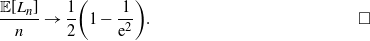
 \begin{equation*}{\mathbb E}\biggl[\frac{ L_{n}}{n}\biggr] \to\frac{1}{2}\biggl( 1-\frac{1}{{\mathrm{e}}^2}\biggr) = 0.432332\ldots .\end{equation*}
Proof. For  $i>1$
, let
$i>1$
, let
 \begin{equation*}\ell_{i,n}=\ln ({\mathbb E}[{\mathbb L}_{i,n}] ) =\ln\biggl(\prod_{j=i+1}^{n}\biggl(1-\frac{2i}{j(j-1)}\biggr)\biggr).\end{equation*}
Using an exact first-order Taylor series expansion of  $\mbox{ln}(1-x)$
around zero, we have
$\mbox{ln}(1-x)$
around zero, we have
 \begin{align*}\ell_{i,n} & =\sum_{j=i+1}^{n}\ln\biggl( 1-\frac{2i}{j(j-1)}\biggr)& =-\sum_{j=i+1}^{n}\frac{2i}{j( j-1) } - \sum_{j=i+1}^{n}\frac{1}{(1 - x_{i,j})^{2}}\biggl( \frac{2i}{j( j-1) }\biggr) ^{2} & =-2\biggl( 1-\frac{i}{n}\biggr) - \sum_{j=i+1}^{n}\frac{1}{(1 - x_{i,j})^{2}}\biggl( \frac{2i}{j( j-1) }\biggr) ^{2} {,}\end{align*}
where each
 \begin{equation*}x_{i,j} \in \biggl(0,\frac{2i}{j(j-1)}\biggr).\end{equation*}
This Taylor series expansion makes it possible to get useful bounds for each  $\ell_{i,n}$
term valid for all
$\ell_{i,n}$
term valid for all  $n > 0$
. Note that the second term of
$n > 0$
. Note that the second term of  $\ell_{i,n}$
is negative, so we immediately have the upper bound
$\ell_{i,n}$
is negative, so we immediately have the upper bound
 \begin{equation*} \ell_{i,n} \leq -2\biggl( 1-\frac{i}{n}\biggr). \end{equation*}
For the lower bound, examine each term in the second summation, and observe that over the range of j in the sum we have
 \begin{equation*}\frac{1}{(1 - x_{i,j})^{2}}\biggl( \frac{2i}{j( j-1) }\biggr) ^{2} \le \frac{1}{(1 - \tfrac{2i}{i(i+1)})^{2}} \biggl( \frac{2i}{ji }\biggr) ^{2}.\end{equation*}
With this bound being valid for  $i>1$
, we establish
$i>1$
, we establish
 \begin{equation*}\frac{1}{(1 - x_{i,j})^{2}}\biggl( \frac{2i}{j( j-1) }\biggr) ^{2} \leq \frac{1}{(1 - \tfrac{2}{(2+1)})^{2}} \biggl( \frac{2}{j }\biggr) ^{2}\le \frac {36} {i^2}.\end{equation*}
We can now use these bounds to sandwich the fraction of leaves:
 \begin{equation*}\frac{1}{n}\sum_{i=2}^{n} \,{\mathrm{e}}^{-2( 1-{{i}/{n}}) - {{36}/{i^2}}}\le \frac{{\mathbb E}[L_{n}]}{n} = \frac{1}{n}\sum_{i=2}^{n} \,{\mathrm{e}}^{\ell_{i,n}} \leq \frac{1}{n}\sum_{i=1}^{n} \,{\mathrm{e}}^{-2( 1-{{i}/{n}}) }.\end{equation*}
The upper bound can be simplified by summing it as a geometric series, which gives
 \begin{align*} \frac{{\mathbb E}[L_{n}]}{n} & \le \frac{{\mathrm{e}}^{-2}}{n}\sum_{i=1}^{n}\,{\mathrm{e}}^{{{2i}/{n}} }\\[3pt]
& = \frac{{\mathrm{e}}^{-2}}{n} \biggl(\frac {{\mathrm{e}}^{2(n+1)/n} -1} {{\mathrm{e}}^{2/n} -1}\biggr)\\[3pt]
& = \frac{{\mathrm{e}}^{-2}}{n} \biggl(\frac {{\mathrm{e}}^{2(n+1)/n} -1} {(1 + 2/n + O(n^{-2})) -1} \biggr) \\[3pt]
&\to \frac 1 2 \biggl(1 - \frac 1 {{\mathrm{e}}^2} \biggr). \end{align*}
\begin{align*} \frac{{\mathbb E}[L_{n}]}{n} & \le \frac{{\mathrm{e}}^{-2}}{n}\sum_{i=1}^{n}\,{\mathrm{e}}^{{{2i}/{n}} }\\[3pt]
& = \frac{{\mathrm{e}}^{-2}}{n} \biggl(\frac {{\mathrm{e}}^{2(n+1)/n} -1} {{\mathrm{e}}^{2/n} -1}\biggr)\\[3pt]
& = \frac{{\mathrm{e}}^{-2}}{n} \biggl(\frac {{\mathrm{e}}^{2(n+1)/n} -1} {(1 + 2/n + O(n^{-2})) -1} \biggr) \\[3pt]
&\to \frac 1 2 \biggl(1 - \frac 1 {{\mathrm{e}}^2} \biggr). \end{align*}
The extraction of the asymptotics from the lower bound is a little more involved. First expand the term  $\exp(-36/i^2)$
in series with an explicit first term and an error of the exact order
$\exp(-36/i^2)$
in series with an explicit first term and an error of the exact order  $1/i^2$
. This means that there is a starting index value
$1/i^2$
. This means that there is a starting index value  $i_0$
and a positive constant K such that the error is at most
$i_0$
and a positive constant K such that the error is at most  $K/i^2$
, for all
$K/i^2$
, for all  $i \ge i_0$
. We can then split the series at
$i \ge i_0$
. We can then split the series at  $i_0$
, getting
$i_0$
, getting
 \begin{align*}\frac{{\mathbb E}[L_{n}]}{n} &\ge \frac{1}{n}\sum_{i=2}^{n} \,{\mathrm{e}}^{-2 (1-{{i}/{n}}) - {{36}/{i^2}}}\\[3pt]
&\ge \frac 1 n \biggl(\sum_{i=2}^{i_0 - 1} \,{\mathrm{e}}^{-2( 1-{{i}/{n}}) } \biggl(1 - \frac {K_{i}}{i^2} \biggr) + \sum_{i=i_0}^{n} \,{\mathrm{e}}^{-2( 1-{{i}/{n}}) } \biggl(1 - \frac {K}{i^2} \biggr)\biggr) \\[3pt]
&= O\biggl( \frac {1} n\biggr) + \frac{{\mathrm{e}}^{-2}}{n} \biggl(\frac {{\mathrm{e}}^{2(n+1)/n} - {\mathrm{e}}^{2i_0/n}} {{\mathrm{e}}^{2/n} -1}\biggr) \\[3pt]
&= O \biggl( \frac {1} n\biggr) + \frac{{\mathrm{e}}^{-2}}{n} \biggl(\frac {{\mathrm{e}}^{2(n+1)/n} - {\mathrm{e}}^{2i_0/n}} {(1 + 2/n + O(n^{-2})) -1}\biggr)\\ [3pt]
&= O \biggl( \frac {1} n\biggr) + {\mathrm{e}}^{-2} \biggl(\frac {{\mathrm{e}}^{2(n+1)/n} - {\mathrm{e}}^{2i_0/n}} {2 + O(n^{-1})}\biggr)\\[3pt]
&\to \frac{1}{2}\biggl(1-\frac{1}{{\mathrm{e}}^2}\biggr) .\end{align*}
\begin{align*}\frac{{\mathbb E}[L_{n}]}{n} &\ge \frac{1}{n}\sum_{i=2}^{n} \,{\mathrm{e}}^{-2 (1-{{i}/{n}}) - {{36}/{i^2}}}\\[3pt]
&\ge \frac 1 n \biggl(\sum_{i=2}^{i_0 - 1} \,{\mathrm{e}}^{-2( 1-{{i}/{n}}) } \biggl(1 - \frac {K_{i}}{i^2} \biggr) + \sum_{i=i_0}^{n} \,{\mathrm{e}}^{-2( 1-{{i}/{n}}) } \biggl(1 - \frac {K}{i^2} \biggr)\biggr) \\[3pt]
&= O\biggl( \frac {1} n\biggr) + \frac{{\mathrm{e}}^{-2}}{n} \biggl(\frac {{\mathrm{e}}^{2(n+1)/n} - {\mathrm{e}}^{2i_0/n}} {{\mathrm{e}}^{2/n} -1}\biggr) \\[3pt]
&= O \biggl( \frac {1} n\biggr) + \frac{{\mathrm{e}}^{-2}}{n} \biggl(\frac {{\mathrm{e}}^{2(n+1)/n} - {\mathrm{e}}^{2i_0/n}} {(1 + 2/n + O(n^{-2})) -1}\biggr)\\ [3pt]
&= O \biggl( \frac {1} n\biggr) + {\mathrm{e}}^{-2} \biggl(\frac {{\mathrm{e}}^{2(n+1)/n} - {\mathrm{e}}^{2i_0/n}} {2 + O(n^{-1})}\biggr)\\[3pt]
&\to \frac{1}{2}\biggl(1-\frac{1}{{\mathrm{e}}^2}\biggr) .\end{align*}
Given the convergence of the upper and lower bounds, the sandwich theorem ascertains that
 \begin{equation*} \hspace*{150pt} \frac{{\mathbb E}[L_{n}]}{n} \to \frac{1}{2}\biggl(1-\frac{1}{{\mathrm{e}}^2}\biggr). \hspace*{125pt}\qed\end{equation*}
We can strengthen this expected fraction result into convergence in  ${\mathcal L}^{2}$
, and thus in probability, too. We need the following result from the theory of consistent estimators in statistics.
${\mathcal L}^{2}$
, and thus in probability, too. We need the following result from the theory of consistent estimators in statistics.
Lemma 5.4. Let  $\{X_{n}\}$
be a sequence of random variables with
$\{X_{n}\}$
be a sequence of random variables with  ${\mathbb E}[ X_{n}^{2}] <\infty$
, for all
${\mathbb E}[ X_{n}^{2}] <\infty$
, for all  $n\ge 1$
. If
$n\ge 1$
. If  ${\mathbb E}[X_{n}] \to \mu\in \mathbb{R} $
and
${\mathbb E}[X_{n}] \to \mu\in \mathbb{R} $
and  $\operatorname{Var} [X_{n}] \to 0$
, then
$\operatorname{Var} [X_{n}] \to 0$
, then  $X_{n}\buildrel {\mathcal L}^{2} \over \longrightarrow \mu\in \mathbb{R}$
.
$X_{n}\buildrel {\mathcal L}^{2} \over \longrightarrow \mu\in \mathbb{R}$
.
Proof. See Theorem 8.2 of [12, pages 54–55].
We also use the fact that for random variables with bounded variance and non-positive correlations, the variability of the average goes to zero.
Lemma 5.5. Let  $\{B_{n}\}$
be a sequence of random variables with non-positive correlations and
$\{B_{n}\}$
be a sequence of random variables with non-positive correlations and  $\operatorname{Var} [ B_{n}] \le M$
, for some
$\operatorname{Var} [ B_{n}] \le M$
, for some  $M > 0$
, then
$M > 0$
, then
 \begin{equation*} \operatorname{Var} \biggl[\sum_{i=1}^{n} \frac{B_{i}}{n} \biggr] \to 0.\end{equation*}
Proof. For each  $B_{n}$
we have
$B_{n}$
we have  $\operatorname{Var} [B_{n}] \le M$
and
$\operatorname{Var} [B_{n}] \le M$
and  $\operatorname{Cov} [B_{i},B_{j}] \le 0$
for
$\operatorname{Cov} [B_{i},B_{j}] \le 0$
for  $i \neq j$
, so we have
$i \neq j$
, so we have
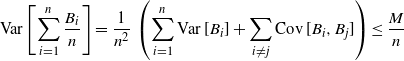 \begin{equation*} \operatorname{Var} \biggl[\sum_{i=1}^{n} \frac{B_{i}}{n} \biggr] = \frac{1}{n^{2}}\, \biggl( \sum_{i=1}^{n} \operatorname{Var} [B_{i}] + \sum_{i \neq j} \operatorname{Cov} [B_{i},B_{j}] \biggr) \le \frac{M}{n}\end{equation*}
and
 \begin{equation*} \hspace*{150pt}\lim_{n\to\infty} \operatorname{Var} \biggl[\sum_{i=1}^{n} \frac{B_{i}}{n} \biggr] = 0. \hspace*{125pt}\qed\end{equation*}
Finally, this gives us our main result.
 \begin{equation*}\frac{ L_{n}}{n} \buildrel {\mathcal L}^{2} \over \longrightarrow\frac{1}{2}\biggl( 1-\frac{1}{{\mathrm{e}}^2}\biggr) = 0.432332\ldots .\end{equation*}
Proof. The result follows immediately by noting the non-positive covariance between the  ${\mathbb L}_{i,n}$
, as in Theorem 5.1, and applying the previous two lemmas to
${\mathbb L}_{i,n}$
, as in Theorem 5.1, and applying the previous two lemmas to  ${{ L_{n}}/{n}}$
.
${{ L_{n}}/{n}}$
.
From the  ${\mathcal L}^{2}$
convergence we get the following.
${\mathcal L}^{2}$
convergence we get the following.
 \begin{equation*}\frac{L_{n}}{n} \buildrel a.s. \over \longrightarrow \frac{1}{2} \biggl( 1-\frac{1}{{\mathrm{e}}^2}\biggr) .\end{equation*}
Proof. In-probability convergence is immediate since  ${\mathcal L}^{p}$
convergence for any
${\mathcal L}^{p}$
convergence for any  $p>0$
implies in-probability. The almost-sure result follows from the fact that in-probability convergence is equivalent to almost-sure convergence for countable probability spaces (see [5, Chapter 2, Section 2] for a discussion).
$p>0$
implies in-probability. The almost-sure result follows from the fact that in-probability convergence is equivalent to almost-sure convergence for countable probability spaces (see [5, Chapter 2, Section 2] for a discussion).
6. Insertion depth
In this section we derive results about random insertion depth under young-age preferential attachment. We let  $D_n$
denote the depth of the node labeled n in a young-age attachment tree. We first find the exact moment generating function, from which the exact distribution and a miscellany of asymptotic results follow.
$D_n$
denote the depth of the node labeled n in a young-age attachment tree. We first find the exact moment generating function, from which the exact distribution and a miscellany of asymptotic results follow.
Let  $T_{n}$
be the tree existing right after node n enters. We condition on
$T_{n}$
be the tree existing right after node n enters. We condition on  $T_{n-1}$
, for some
$T_{n-1}$
, for some  $t\in\mathbb{R}$
, and use the young-age probability model (2.1) to write
$t\in\mathbb{R}$
, and use the young-age probability model (2.1) to write
 \begin{equation*}{\mathbb E}[ {\mathrm{e}}^{D_{n}t} \mid T_{n-1}] =\sum_{k=1}^{n-1}\,{\mathrm{e}}^{( D_{k}+1) t}\frac{2k}{n(n-1)}.\end{equation*}
Taking expectation of both sides and using the law of iterated expectations, we arrive at a recursive equation for the moment generating function of  $D_{n}$
:
$D_{n}$
:
 \begin{equation*}\phi_{D_{n}}(t) =\sum_{k=1}^{n-1}{\mathbb E}[ {\mathrm{e}}^{(D_{k}+1) t}] \, \frac{2k}{n( n-1) } = 2 {\mathrm{e}}^t\sum_{k=1}^{n-1}\phi_{D_{k}}( t) \, \frac k {n(n-1) }.\end{equation*}
Differencing, we obtain
 \begin{equation*} n(n-1) \phi_{D_{n}}(t) - (n-1)(n-2) \phi_{D_{n-1}}(t) =2{\mathrm{e}}^t( n-1)\, \phi_{D_{n-1}}(t).\end{equation*}
After refactoring, we have
 \begin{equation*}\phi_{D_{n}}(t) = \biggl(\frac{n-2+2{\mathrm{e}}^t}{n}\biggr)\phi_{D_{n-1}}(t).\end{equation*}
Iterating this relation back, we get
 \begin{equation*}\phi_{D_{n}}( t) = \biggl(\prod_{j=1}^{n-2}\frac{j+2{\mathrm{e}}^t}{j+2}\biggr)\,\phi_{D_{2}}(t).\end{equation*}
We have  $\phi_{D_{2}}(t)={\mathrm{e}}^t$
and
$\phi_{D_{2}}(t)={\mathrm{e}}^t$
and  $\phi_{D_{1}}(t)=1$
as boundary conditions. It follows that
$\phi_{D_{1}}(t)=1$
as boundary conditions. It follows that
 \begin{equation*}\phi_{D_{n}}(t) = \frac{\prod_{j=1}^{n-2}( j+2{\mathrm{e}}^t)}{n!}\, 2{\mathrm{e}}^t =\frac{1}{n!}\prod_{j=0}^{n-2}(j+2{\mathrm{e}}^t) \quad \text{for } n\ge 2.\end{equation*}
We express the the next theorem in terms of the unsigned Stirling numbers of the first kind, which are coefficients in the polynomial representing the rising factorial:
 \begin{equation*} x (x+1) \cdots (x+n-1) =\sum_{k=0}^{n}\biggl[\begin{matrix}n\\ k \end{matrix}\biggr]x^k,\end{equation*}
Theorem 6.1. Let  $D_n$
be the depth of the nth node in a young-age attachment tree. The exact distribution of this insertion depth is
$D_n$
be the depth of the nth node in a young-age attachment tree. The exact distribution of this insertion depth is
 \begin{equation*}{\mathbb P}(D_{n}=k) =\frac{2^{k}}{n!}\biggl[\begin{matrix}n-1\\ k \end{matrix}\biggr], \quad k=1,\ldots,n-1.\end{equation*}
Proof. Using the moment generating function presented right before the theorem, we can derive the exact probability mass function of  $D_{n}$
. Setting
$D_{n}$
. Setting  $t = \ln u$
in the moment generating function switches the view to the probability generating function
$t = \ln u$
in the moment generating function switches the view to the probability generating function  $\zeta_n(u)$
. Namely, it is
$\zeta_n(u)$
. Namely, it is
 \begin{equation*}\zeta_n(u) = \phi_{n}(\ln u) =\frac{2u( 2u+1) \cdots( 2u+n-2) }{n!}.\end{equation*}
Hence we have
 \begin{equation*} \zeta_n(u) =\frac{1}{n!}\sum_{k=0}^{n-1} \biggl[\begin{matrix}n-1\\ k \end{matrix} \biggr](2u)^{k}.\end{equation*}
The exact distribution of  $D_n$
is obtained by extracting coefficients.
$D_n$
is obtained by extracting coefficients.
The exact distribution of the nth insertion depth in young-age recursive trees is the same as its counterpart in random binary search trees. Hence a number of results follow immediately, which we list without proof. The interested reader can examine Chapter 2 in [Reference Mahmoud13]. In the following proposition, all asymptotics are taken as  $n\to\infty$
.
$n\to\infty$
.
Proposition 6.1. Let  $D_n$
be the depth of insertion of the nth node in a young-age preferential attachment tree. We have
$D_n$
be the depth of insertion of the nth node in a young-age preferential attachment tree. We have
 \begin{gather*}\begin{aligned}{\mathbb E}[D_{n}] &=2(H_{n}-1) \sim 2\ln n,\\[4pt]
\operatorname{Var} [D_{n}] &= 2(H_{n}+1) - 4H_{n}^{(2)} \sim 2\ln n,\end{aligned}\\[4pt]
\frac{D_{n}}{\ln n}\buildrel {\mathcal L}^{2} \over \longrightarrow 2, \quad \frac{D_{n}}{\ln n}\buildrel a.s. \over \longrightarrow 2,\\[4pt]
\frac{D_{n}-2\ln n}{\sqrt{2\ln n}} \buildrel d \over \longrightarrow N(0,1). \end{gather*}
\begin{gather*}\begin{aligned}{\mathbb E}[D_{n}] &=2(H_{n}-1) \sim 2\ln n,\\[4pt]
\operatorname{Var} [D_{n}] &= 2(H_{n}+1) - 4H_{n}^{(2)} \sim 2\ln n,\end{aligned}\\[4pt]
\frac{D_{n}}{\ln n}\buildrel {\mathcal L}^{2} \over \longrightarrow 2, \quad \frac{D_{n}}{\ln n}\buildrel a.s. \over \longrightarrow 2,\\[4pt]
\frac{D_{n}-2\ln n}{\sqrt{2\ln n}} \buildrel d \over \longrightarrow N(0,1). \end{gather*}
7. Conclusion
The non-uniform young-age attachment model introduced has both similarities to and differences from the standard uniform model. As seen in Proposition 6.1, the average and variance of the insertion depth in these trees is double that of the uniform case – and both random trees live in the ‘small world’. Like the uniform model, the insertion depth in the young-age model is also asymptotically normal (Proposition 6.1).
In the case of tree leaves and outdegrees, the young-age model differs substantially from the uniform model. The asymptotic fraction of leaves in young-age attachment trees is significantly less than 1/2 (the asymptotic fraction in uniform recursive trees), while in the limit the outdegrees are Poisson or ‘near-Poisson’. These facts imply that the nodes in the young-age model have a better chance of recruiting than the uniform case, but they tend to have ‘sparse’ connections with fewer outnode links.
The young-age model generates some natural directions for future research. Does the behavior carry over to probability models driven by different powers of the node index? Such an attachment mechanism could be used to model networks with varying degrees of age-based affinity. For example, one can work with a general class of growth models in which
 \begin{equation*} {\mathbb P}({\mathcal A}_{i,n}) \sim i^{\alpha} \quad \text{for } 1\le i\le n-1, \quad \alpha \in \mathbb{R}.\end{equation*}
The growth index  $\alpha$
would be a parameter of interest and could be estimated from empirical data under different sampling schemes. Preliminary work suggests that, as
$\alpha$
would be a parameter of interest and could be estimated from empirical data under different sampling schemes. Preliminary work suggests that, as  $\alpha$
grows, asymptotic normality remains for the insertion depth albeit with a different character of the variance. For large
$\alpha$
grows, asymptotic normality remains for the insertion depth albeit with a different character of the variance. For large  $\alpha$
, the growth model approaches the complete linear chaining of the nodes.
$\alpha$
, the growth model approaches the complete linear chaining of the nodes.
Acknowledgement
We thank the referees for thoughtful reports and constructive criticism.

