


1. INTRODUCTION
With the advent of high power lasers, it has become possible to study the interaction of free electrons with high intensity laser pulses. By “high intensity” laser field E0 of center carrier frequency ω0, we mean that it satisfies the condition: a 0 ≥ 1, where  At these intensities electron quiver velocities are close to the velocity of light and the motion of even free electrons becomes highly nonlinear. The nonlinear laser-plasma interaction gives rise to a variety of phenomena like X-ray generation (Kieffer et al., Reference Kieffer, Matte, Pépin, Chaker, Beaudoin, Johnston, Chien, Coe, Mourou and Dubau1992), γ-ray generation (Norreys et al., Reference Norreys, Santala, Clark, Zepf, Watts, Beg, Krushelnick, Tatarakis, Dangor, Fang, Graham, McCanny, Singhal, Ledingham, Creswell, Sanderson, Magill, Machacek, Wark, Allott, Kennedy and Neely1999) relativistic self-focusing (Sprangle, Reference Sprangle1987), high-harmonic generation (Linde, Reference Linde1999; Nuzzo et al., Reference Nuzzo, Zarcone, Ferrante and Basile2000; Villoresi et al., Reference Villoresi, Barbiero, Poletto, Nisoli, Cerullo, Priori, Stagira, De Lisco, Bruzzese and Altucci2001; Nisoli et al., Reference Nisoli, Sansone, Stagira, Silvestri, Vozzi, Pascolini, Poletto, Villoresi and Tondello2003; Foldes et al., Reference Foldes, Kocsis, Racz, Szatmari and Veres2003; Bulanov et al., Reference Bulanov, Esirkepov, Naumova and Sokolov2003; Baeva et al., Reference Baeva, Gordienko and Pukhov2006; Gupta et al., Reference Gupta, Sharma and Mahmoud2007; Varró, Reference Varró2007; Ganeev, Reference Ganeev2009), electron and proton acceleration (Malka et al., Reference Malka, Fritzler, Lefebvre, Aleonard, Burgy, Chambaret, Chemin, Krushelnick, Malka, Mangles, Najmudin, Pittman, Rousseau, Scheurer, Walton and Dangor2002; Zepf et al., Reference Zepf, Clark, Beg, Clarke, Dangor, Gopal, Krushelnick, Norreys, Tatarakis, Wagner and Wei2003; Bingham et al., Reference Bingham, Mendonça and Shukla2004). When such an intense laser is incident on a thin metal layer, an ultrathin, highly inhomogeneous dense plasma layer is created. The electromagnetic field is almost localized in a narrow region in the vicinity of the boundary, which can be modeled as a thin plasma slab. Laser pulse interaction with a very thin slab of over-dense plasma brings in new features that are not encountered in underdense plasmas (Vshivkov et al., Reference Vshivkov, Naumova, Pegoraro and Bulanov1998). These effects show up prominently when the incident laser pulse contains only few-cycles.
In the present work, we consider an ultrashort few-cycle laser pulse having central carrier frequency ω0, wave vector ![]() , and dimensionless amplitude a 0 ncident on a thin plasma layer. The thickness l of the layer is assumed to be much smaller than the average skin depth of incoming radiation and wavelength of laser. The laser pulse is assumed to be p-polarized transverse magnetic (TM) wave. The electron plasma frequency ωp is greater than ω0. The plasma density varies from solid to vacuum in a distance less than the wavelength. As a result of the interaction of laser pulse with such highly inhomogeneous plasma, the surface electromagnetic waves on plasma-vacuum interface are generated (Dromey et al., Reference Dromey, Kar, Bellei, Carroll, Clarke, Green, Kneip, Markey, Nagel, Simpson, Willingale, McKenna, Neely, Najmudin, Krushelnick, Norreys and Zepf2007; Bulanov et al., Reference Bulanov, Macchi, Maksimchuk, Matsuoka, Nees and Pegoraro2007). The character of surface waves depends on the boundary conditions, which must supplement the field equations.
, and dimensionless amplitude a 0 ncident on a thin plasma layer. The thickness l of the layer is assumed to be much smaller than the average skin depth of incoming radiation and wavelength of laser. The laser pulse is assumed to be p-polarized transverse magnetic (TM) wave. The electron plasma frequency ωp is greater than ω0. The plasma density varies from solid to vacuum in a distance less than the wavelength. As a result of the interaction of laser pulse with such highly inhomogeneous plasma, the surface electromagnetic waves on plasma-vacuum interface are generated (Dromey et al., Reference Dromey, Kar, Bellei, Carroll, Clarke, Green, Kneip, Markey, Nagel, Simpson, Willingale, McKenna, Neely, Najmudin, Krushelnick, Norreys and Zepf2007; Bulanov et al., Reference Bulanov, Macchi, Maksimchuk, Matsuoka, Nees and Pegoraro2007). The character of surface waves depends on the boundary conditions, which must supplement the field equations.
Varró (Reference Varró2007) has shown that in the scattered radiation generated by an ultrashort, intense, few-cycle laser pulse impinging on a metal nano-layer, nonoscillatory Wakefield appears with a definite sign. This quasistatic field remains for many more periods of the main pulse. In this paper, we analyze the effect of the pulse-shape on the excitation of the quasistatic Wakefield. We find that the magnitude and sign of this left-over field depends on the pulse-shape, carrier envelope phase (CEP), thickness of the plasma layer, angle of incidence of the laser and gradient of the plasma density. The pulse-shapes considered are Gaussian, Lorentzian, and hyperbolic secant having identical full width at half maximum (FWHM) of intensity. Following Brabec and Krausz (Reference Brabec and Krausz1997, Reference Brabec and Krausz2000), we have made use of the powerful concept of the envelope for few-cycle laser pulses up to the limit of single cycle.
Generation of high harmonics from a solid target can be understood in terms of coherent wake emission (CWE) (Quéré et al., Reference Quéré, Thaury, Monot, Dobosz and Martin2006; Brügge & Pukhov, Reference Brügge and Pukhov2007; Dromey et al., Reference Dromey, Rykovanov, Adams, Hörlein, Nomura, Carroll, Foster, Kar, Markey, McKenna, Neely, Geissler, Tsakiris and Zepf2009). CWE mechanism is predominant at moderately relativistic intensities (a 0 ~ 1) and short, but finite plasma gradient lengths. Because of the density inhomogeneity, the electrostatic oscillations couple back to electromagnetic modes. A transient phase matching between the electromagnetic field and plasma oscillations with a density gradient leads to the emission of harmonics of the incident frequency (Quéré et al., Reference Quéré, Thaury, Monot, Dobosz and Martin2006, Reference Quéré, Thaury, Geindre, Bonnaud, Monot and Martin2008). Relativistic effects modify the nonlinear processes that are known in the limit of moderate radiation amplitudes. In this paper, we consider the reflection and transmission of an oblique incident electromagnetic few-cycle laser pulse from a highly inhomogeneous plasma layer following the model introduced by Varró (Reference Varró2007). This model includes radiation reaction term resulting in phenomenological damping in the equation of motion of the plasma layer. In the present study, we follow the same model that include the effect of the specific pulse-shape, angle of incidence, CEP of the laser pulse, number of cycles in a pulse on the high harmonic generation.
The paper is organized as follows: In section 2, we analyze the dependence of the quasistatic Wakefield on the pulse-shape of an ultrashort, intense, few cycle laser in the reflected radiation from a thin, dense plasma layer. Dependence of high harmonic generation on the pulse-shape of an ultrashort, intense, few cycle laser in the reflected radiation from a thin, dense plasma layer is given in Section 3. Results and discussion are presented in Section 4. Finally, Section 5 presents our conclusions.
2. DEPENDENCE OF QUASISTATIC WAKEFIELDS ON THE PULSE SHAPE OF AN ULTRASHORT, INTENSE, FEW CYCLE LASER IN THE REFLECTED RADIATION FROM A THIN, DENSE PLASMA LAYER
We consider an ultrashort few-cycle laser pulse with central carrier frequency ω0, wave vector ![]() , and dimensionless amplitude
, and dimensionless amplitude ![]() , impinging on a plasma thin layer, lying between
, impinging on a plasma thin layer, lying between ![]() and
and ![]() , is located at x = 0, here e and m denote the charge and rest mass of the electron, respectively. The thickness l of the plasma layer is assumed to be much smaller than the average skin depth of incoming radiation. The wave vector
, is located at x = 0, here e and m denote the charge and rest mass of the electron, respectively. The thickness l of the plasma layer is assumed to be much smaller than the average skin depth of incoming radiation. The wave vector ![]() makes an angle θ with the z-axis. The plane of incidence is y–z plane. The laser pulse is assumed to be p-polarized TM wave with electric fields
makes an angle θ with the z-axis. The plane of incidence is y–z plane. The laser pulse is assumed to be p-polarized TM wave with electric fields ![]() and magnetic field
and magnetic field ![]() . The plasma density N drops to zero over a length much less than laser wavelength. In over-dense plasma the penetration length of the electromagnetic wave,
. The plasma density N drops to zero over a length much less than laser wavelength. In over-dense plasma the penetration length of the electromagnetic wave, ![]() is small compared to its wavelength in vacuum λ. Here c is the speed of light in vacuum, and
is small compared to its wavelength in vacuum λ. Here c is the speed of light in vacuum, and ![]() is the plasma frequency. The interaction of the laser with thin plasma layer gives rise to the generation of surface electromagnetic waves on a semi-bounded plasma-vacuum interface. The character of surface waves essentially depends on the boundary conditions, which must supplement the field equations. The dimensionless parameter
is the plasma frequency. The interaction of the laser with thin plasma layer gives rise to the generation of surface electromagnetic waves on a semi-bounded plasma-vacuum interface. The character of surface waves essentially depends on the boundary conditions, which must supplement the field equations. The dimensionless parameter ![]() , gives a measure of the transparency (k ≪1) or opaqueness (k ≫1) of the plasma layer.
, gives a measure of the transparency (k ≪1) or opaqueness (k ≫1) of the plasma layer.
Following Varró (Reference Varró2007), the reflected field f 1 (t′) from thin plasma layer in the region-1(![]() ) can be represented in terms of the y-component of the local velocity
) can be represented in terms of the y-component of the local velocity ![]()
![]() , of the electrons in the plasma layer:
, of the electrons in the plasma layer:
Where ![]() is the retarded time,
is the retarded time, ![]()
![]() is the damping parameter.
is the damping parameter.
The local velocity ![]() is obtained by solving the following equation of motion for electrons in presence of complete electric field:
is obtained by solving the following equation of motion for electrons in presence of complete electric field:
![{d^2 {\rm \delta}_y \lpar t^{\prime}\rpar \over dt^{\prime 2}} = \cos {\rm \theta} \left[{e \over m} F \lpar t^{\prime}\rpar - {\rm \Gamma} \left({d{\rm \delta}_y \lpar t^{\prime}\rpar \over dt^{\prime}} \right)\right]\eqno\lpar 2\rpar](https://static.cambridge.org/binary/version/id/urn:cambridge.org:id:binary:20151021092105787-0842:S0263034610000741_eqn2.gif?pub-status=live)
where F(t) represents the field of the incident laser pulse.
We consider various analytic pulse-shapes, ![]() where A(t) is the envelope of the pulse. The envelopes for a Gaussian, Lorentzian, and hyperbolic secant pulses are taken to be
where A(t) is the envelope of the pulse. The envelopes for a Gaussian, Lorentzian, and hyperbolic secant pulses are taken to be ![]() ,
, ![]() , and
, and ![]() , respectively, where τ is FWHM of pulse intensity and ϕ is carrier envelope phase (Brabec & Krausz, Reference Brabec and Krausz1997).
, respectively, where τ is FWHM of pulse intensity and ϕ is carrier envelope phase (Brabec & Krausz, Reference Brabec and Krausz1997).
Solving Eq. (2), the asymptotic behavior of the local velocity ![]() , for different temporal envelopes of the laser pulse, can be expressed as:
, for different temporal envelopes of the laser pulse, can be expressed as:
![\eqalign{\left[{d{\rm \delta}_y \lpar t^{\prime}\rpar \over dt^{\prime}} \right]_g &\approx {e\cos {\rm \theta} \over m} \exp \left(- t^{\prime }\Gamma \cos {\rm \theta} \right){F_0 {\rm \tau} \sqrt {\rm \pi} \over 1.17} \cr &\quad \times \exp \left\{- {{\rm \tau}^2 \left({\rm \omega}_0^2 - {\rm \Gamma}^2 \cos^2 {\rm \theta} \right)\over 5.4756} \right\}\cr &\quad \times \cos \left\{{\rm \phi} + {k{\rm \omega}_0^2 {\rm \tau}^2 \cos {\rm \theta} \over 2.7378} \right\}.}](https://static.cambridge.org/binary/version/id/urn:cambridge.org:id:binary:20151021092105787-0842:S0263034610000741_eqnU1.gif?pub-status=live)
For Lorentzian pulse:
![\eqalign{\left[{d{\rm \delta}_y \lpar t^{\prime}\rpar \over dt^{\prime}} \right]_l &\approx {e\cos {\rm \theta} \over m} \exp \left(- t^{\prime}{\rm \Gamma} \cos {\rm \theta} \right){F_0 {\rm \tau \pi} \over 1.29} \cos \lpar {\rm \phi}\rpar \cr &\quad \times \exp \left\{- {{\rm \tau} \left({\rm \omega}_0^2 + {\rm \Gamma}^2 \cos^2 {\rm \theta} \right)^{{1 / 2}} \over 1.29} \right\}.}](https://static.cambridge.org/binary/version/id/urn:cambridge.org:id:binary:20151021092105787-0842:S0263034610000741_eqnU2.gif?pub-status=live)
For hyperbolic secant pulse:
![\eqalign{\left[{d{\rm \delta}_y \lpar t^{\prime}\rpar \over dt^{\prime}} \right]_h &\approx {e\cos {\rm \theta} \over m} \exp \left(- t^{\prime }\Gamma \cos {\rm \theta} \right){F_0 {\rm \tau \pi} \over 3.52} \cr &\quad \times \left[e^{i {\rm \phi}} \sec h\left\{{{\rm \tau \pi} \over 3.52} \left({\rm \omega}_0 - i {\rm \Gamma} \cos {\rm \theta} \right)\right\}\right. \cr &\quad \left. + e^{ - i{\rm \phi}} \sec h\left\{- {{\rm \tau \pi} \over 3.52} \left({\rm \omega}_0 + i{\rm \Gamma} \cos {\rm \theta} \right)\right\}\right]}.](https://static.cambridge.org/binary/version/id/urn:cambridge.org:id:binary:20151021092105787-0842:S0263034610000741_eqnU3.gif?pub-status=live)
Substituting these values of ![]() in Eq. (1), we find that the decay time of the reflected field f 1 (t′) is
in Eq. (1), we find that the decay time of the reflected field f 1 (t′) is ![]() . For proper choice of the plasma density, angle of incidence, thickness of the plasma layer, t 0 can be much larger than the period of the main pulse. This field embodies the reflected main few-cycle pulse along with the left over field, which persists after the passage of the main pulse. This Wakefield is quasistatic and its magnitude depends on CEP, angle of incidence, plasma layer parameters, pulse-shape, and number of cycles in the laser pulse. An analytic expression for the frozen-in Wakefield has been derived by Varró (Reference Varró2007) in the approximation in which the duration of the Wakefield has been assumed to be infinite. However, in this approximation, the specific effect of pulse-shape is smeared out. In order to include the effect of pulse-shape on the reflected field, we solve the equation of motion exactly by employing the fifth order Runge-Kutta method. We find that the magnitude of the quasistatic frozen-in electric field (Wakefield) is about 10−3–10−4 of the main pulse. The numerical results are shown in Figures 1, 2, and 3.
. For proper choice of the plasma density, angle of incidence, thickness of the plasma layer, t 0 can be much larger than the period of the main pulse. This field embodies the reflected main few-cycle pulse along with the left over field, which persists after the passage of the main pulse. This Wakefield is quasistatic and its magnitude depends on CEP, angle of incidence, plasma layer parameters, pulse-shape, and number of cycles in the laser pulse. An analytic expression for the frozen-in Wakefield has been derived by Varró (Reference Varró2007) in the approximation in which the duration of the Wakefield has been assumed to be infinite. However, in this approximation, the specific effect of pulse-shape is smeared out. In order to include the effect of pulse-shape on the reflected field, we solve the equation of motion exactly by employing the fifth order Runge-Kutta method. We find that the magnitude of the quasistatic frozen-in electric field (Wakefield) is about 10−3–10−4 of the main pulse. The numerical results are shown in Figures 1, 2, and 3.
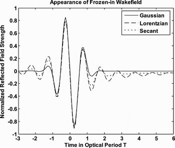
Fig. 1. Shows the appearance of frozen-in Wakefield originating from a single cycle incident laser pulse having different pulse-shape. The angle of incidence in each case is 56 degree, and CE phase = 0. Bold line represents the magnitude of the field from the laser pulse with Gaussian, dashed line for Lorentzian, and the dotted line for hyperbolic secant pulse-shape. The thickness of metal layer is 2 mm, λ = 800 nm, center carrier frequency ![]() , free electron density is 1022 cm−3 and the electric field strength of the reflected signal is normalized by
, free electron density is 1022 cm−3 and the electric field strength of the reflected signal is normalized by ![]() (F0 is the peak value of the incoming laser field).
(F0 is the peak value of the incoming laser field).
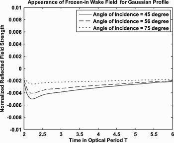
Fig. 2. Represents the variation of the frozen-in Wakefields reflected field strength as a function of normalized retarded time with angles of incidence as parameter corresponding to the incident Gaussian pulse-shape. The CE phase has been chosen to be zero. The thickness of metal layer is 2 mm, free electron density is 1022 cm−3, λ = 800 nm, l = 2 nm, center carrier frequency ![]() , and the electric field strength of the reflected signal is normalized by
, and the electric field strength of the reflected signal is normalized by ![]() .
.
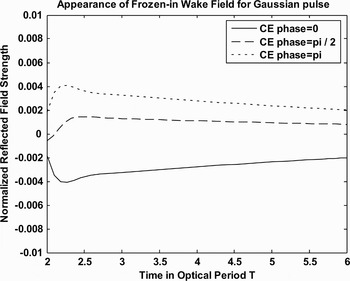
Fig. 3. Shows the variation of the Wakefields as a function of normalized retarded time with CE phase as parameter corresponding to the incident Gaussian pulse-shape. The angle of incidence has been chosen to be 56 degree, l = 2 mm, free electron density is 1022 cm−3, λ = 800 nm, center carrier frequency ![]() , and the electric field strength of the reflected signal is normalized by
, and the electric field strength of the reflected signal is normalized by ![]() .
.
3. DEPENDENCE OF HIGH HARMONIC GENERATION ON THE PULSE-SHAPE OF AN ULTRASHORT, INTENSE, FEW CYCLE LASER IN THE REFLECTED RADIATION FROM A THIN, DENSE PLASMA LAYER
In the interaction of obliquely incident, ultrashort, ultraintense, few-cycle laser with a thin plasma layer, surface current is generated. The equation of motion of the electron in the plasma is given by ![]() , and
, and ![]() where
where ![]() , and
, and ![]() are electric and magnetic field vector associated with the laser light,
are electric and magnetic field vector associated with the laser light, ![]() is the local velocity of the electron, and γ is the relativistic factor given by
is the local velocity of the electron, and γ is the relativistic factor given by ![]() . Solving equation of motion of the electron for the component of displacement vector perpendicular and parallel to
. Solving equation of motion of the electron for the component of displacement vector perpendicular and parallel to ![]() denoted by
denoted by ![]() and
and ![]() respectively, one obtains:
respectively, one obtains:
and
![{d{\rm \delta}_{\rm II} \over d{\rm \xi}} = {1 \over 2c} \left[\left({d{\rm \delta}_{\bot} \over d{\rm \xi}} \right)^2 \right]. \eqno\lpar 4\rpar](https://static.cambridge.org/binary/version/id/urn:cambridge.org:id:binary:20151021092105787-0842:S0263034610000741_eqn4.gif?pub-status=live)
where ![]() is exact retarded time at the position of the electrons. The y-component of local velocity
is exact retarded time at the position of the electrons. The y-component of local velocity ![]() can be expressed in terms of
can be expressed in terms of ![]() :
:

Fourier transforms of f 1 (ξ) yields the reflected field in frequency domain:
The Fourier transform of local velocity for the Lorentz pulse-shape can be obtained as (Appendix):
![\eqalign{{d{\rm \delta}_y \lpar {\rm \omega}\rpar \over dt^{\prime}} &\approx \exp \left({i{\rm \beta}^2 {\rm \omega \tau \pi} \over 5.16} \right)\times \vint_{- \infty}^{\infty} d{\rm \xi} L\lpar {\rm \xi} \rpar \cr &\quad \times \exp \left[i{\rm \omega \xi} \left(1 + {{\rm \beta}^2 \over 2\left\{1 + \left({1.29{\rm \xi} \over {\rm \tau}} \right)^2 \right\}} \right)\right]\cr &\quad \times \exp \left[i{\rm \omega \beta} ^2 {{\rm \tau} \over 2.58} \tan^{ - 1} \left({1.29 {\rm \xi} \over {\rm \tau}} \right)\right]\comma \; } \eqno\lpar 7\rpar](https://static.cambridge.org/binary/version/id/urn:cambridge.org:id:binary:20151021092105787-0842:S0263034610000741_eqn7.gif?pub-status=live)
where
![\eqalign{&{L\lpar {\rm \xi} \rpar \over c} = \sum_n J_n \left({{\rm \beta}^2 {\rm \omega} \over 2{\rm \omega}_0 \left\{1 + \left({1.29{\rm \xi} \over {\rm \tau}} \right)^2 \right\}^2} \right)\cr &\times \left[ { - i{\rm \beta} \cos {\rm \theta} \over \left\{1 + \left({1.29{\rm \xi} \over {\rm \tau}} \right)^2 \right\}} \left\{e^{iA\lpar 1 - 2n\rpar } - e^{iA\lpar 1 + 2n\rpar } \right\}\right.\cr & \quad + {{\rm \beta}^2 \sin {\rm \theta} \over 2\left\{1 + \left({1.29{\rm \xi} \over {\rm \tau}} \right)^2 \right\}^2} \left\{\matrix{2e^{ - i2nA} - e^{ - i2A\lpar 1 - n\rpar } \cr - e^{ - 2iA\lpar 1 + n\rpar }} \right\}\bigg]} \eqno\lpar 8\rpar](https://static.cambridge.org/binary/version/id/urn:cambridge.org:id:binary:20151021092105787-0842:S0263034610000741_eqn8.gif?pub-status=live)
The value of the Fourier transform of local velocity for the hyperbolic secant pulse-shape is given by (Appendix):
![\eqalign{{d{\rm \delta}_y \lpar {\rm \omega}\rpar \over dt^{\prime}} &\approx \exp \left(- {i{\rm \beta}^2 {\rm \omega \tau} \over 1.76} \right)\times \vint_{- \infty}^{\infty} d{\rm \xi}\ H\lpar {\rm \xi} \rpar \exp \left[i{\rm \omega \xi} \right]\cr &\quad \times \exp \left[i{\rm \omega \beta}^2 {{\rm \tau} \over 1.76} \tanh \left({1.76 {\rm \xi} \over {\rm \tau}} \right)\right]\comma \; } \eqno\lpar 9\rpar](https://static.cambridge.org/binary/version/id/urn:cambridge.org:id:binary:20151021092105787-0842:S0263034610000741_eqn9.gif?pub-status=live)
where
![\eqalign{{H\lpar {\rm \xi}\rpar \over c} &= \sum_n J_n \left[{\rm \beta}^2 {{\rm \omega} \over 2{\rm \omega}_0} \left\{\sec h \left({1.76 {\rm \xi} \over {\rm \tau}} \right)\right\}^2 \right]\cr &\times \left[- i{\rm \beta} \sec h \left({1.76 {\rm \xi} \over {\rm \tau}} \right)\cos {\rm \theta} \left\{e^{iA\lpar 1 - 2n\rpar } - e^{iA\lpar 1 + 2n\rpar } \right\}\right. \cr & \left. + {{\rm \beta}^2 \over 2} \left\{\sec h \left({1.76 {\rm \xi} \over {\rm \tau}} \right)\right\}^2 \sin {\rm \theta} \left\{2e^{ - i2nA} - e^{ - i2A\lpar 1 - n\rpar } - e^{ - 2iA\lpar 1 + n\rpar } \right\}\right] .} \eqno\lpar 10\rpar](https://static.cambridge.org/binary/version/id/urn:cambridge.org:id:binary:20151021092105787-0842:S0263034610000741_eqn10.gif?pub-status=live)
The value of the Fourier transform of local velocity the Gaussian pulse-shape can be expressed as (Appendix):
where ![]() , and
, and
![\eqalign{{G\lpar {\rm \xi}\rpar \over c} &= \sum_n J_n \left[{\rm \beta}^2 {{\rm \omega} \over 2{\rm \omega}_0} \exp \left\{- 2 \left({1.17{\rm \xi} \over {\rm \tau}} \right)^2 \right\}\right]\cr &\quad \times \bigg[ - i{\rm \beta} \cos {\rm \theta} \left\{e^{iA\lpar 1 - 2n\rpar } - e^{iA\lpar 1 + 2n\rpar } \right\} \exp \left\{- \left({1.17{\rm \xi} \over {\rm \tau}} \right)^2 \right\}\cr &\quad +{{\rm \beta}^2 \over 2}\sin {\rm \theta} \left\{2e^{ - i2nA} - e^{ - i2A\lpar 1 - n\rpar } - e^{ - 2iA\lpar 1 + n\rpar } \right\}\cr &\quad \times \exp \left\{- 2\left({1.17{\rm \xi} \over {\rm \tau}} \right)^2 \right\}\bigg] .} \eqno\lpar 12\rpar](https://static.cambridge.org/binary/version/id/urn:cambridge.org:id:binary:20151021092105787-0842:S0263034610000741_eqn12.gif?pub-status=live)
4. RESULTS AND DISCUSSION
We present our results when an intense few-cycle, ultrashort laser pulse interacts with a preformed highly inhomogeneous over-dense thin (thickness of the film l ≪ λ) plasma layer. Numerical results show that there remains a quasistatic left over field. The duration of the existence of the quasistatic Wakefield depends on the optimum choice of the plasma density, thickness of the plasma layer, and angle of incidence. The magnitude and sign of the Wakefield are found to depend on the pulse-shape, number of cycles in the pulse, and CEP. Figure 1 shows the appearance of frozen-in Wakefields caused by single cycle incident laser pulse having Gaussian, Lorentzian, and hyperbolic secant pulse-shape. The relative magnitudes of the Wakefields due to Gaussian, Lorentzian, hyperbolic secant pulse are found to be in the ratio 1:14:12. An explanation for different magnitudes of the fields created can be given in terms of the duration for which the different pulses last. It is noted that the tail of the Lorentzian pulse goes to zero at a slower rate than the other two. Gaussian pulse decreases to zero at the fastest rate. All these pulses have single cycle, and same FWHM. When such pulses are incident on thin plasma layer then pulse front sweeps this surface creating a superluminal polarization wave described by the local displacement. The laser pulse profiles, which have larger interaction time and are in phase with electron motion, can transfer more energy to the electron. Such a coherent motion is responsible for frozen-in Wakefields of varying magnitudes. Figure 2 represents the variation of the frozen-in Wakefields with the retarded time (t′/T) for angles of incidence (θ) corresponding to Gaussian pulse. It is found that with increasing θ, the magnitude of frozen-in Wakefield decreases. This is because, when a single cycle, ultrashort p-polarized TM-laser pulse, is obliquely incident on plasma layer then the y-component of the electric field E y is responsible for frozen in Wakefields. This field is which is proportional to cos θ. Figure 3 depicts the variation of the Wakefield with time (t′/T) keeping the carrier-envelope (CE) phase constant, corresponding to Gaussian pulse. The effects of CE phase are dominant only in the case of laser pulses whose duration is definitely less than about 10 optical cycles. The amplitude and sign of these Wakefields can be modulated by changing the CE phase of the incoming pulse.
The reflected radiation also exhibits the presence of high harmonics of the incident laser pulse. Figure 4 represents the variation of the normalized harmonic intensity with normalized frequency ![]() , when the incident few-cycle (p = 2) pulses are Gaussian. Figures 5.1, 5.2, 5.3 show the generation of high harmonics in reflected spectrum for single cycle (p = 1) pulse corresponding to Gaussian, hyperbolic secant, and Lorentzian pulses respectively. Figure 6 shows the variation of the normalized intensity of the harmonics in the reflected radiation caused by the incident secant laser pulse. Maximum intensity is found at
, when the incident few-cycle (p = 2) pulses are Gaussian. Figures 5.1, 5.2, 5.3 show the generation of high harmonics in reflected spectrum for single cycle (p = 1) pulse corresponding to Gaussian, hyperbolic secant, and Lorentzian pulses respectively. Figure 6 shows the variation of the normalized intensity of the harmonics in the reflected radiation caused by the incident secant laser pulse. Maximum intensity is found at ![]() . Higher harmonics are found with decreasing intensities. Figure 7 depicts the effect of the variation of the CE phase on the intensity of the reflected harmonic at
. Higher harmonics are found with decreasing intensities. Figure 7 depicts the effect of the variation of the CE phase on the intensity of the reflected harmonic at ![]() caused by a single cycle Gaussian pulse. Figure 8 represents the variation of the intensity of the 2ω0 harmonic with angle of incidence caused by a single cycle Gaussian pulse.
caused by a single cycle Gaussian pulse. Figure 8 represents the variation of the intensity of the 2ω0 harmonic with angle of incidence caused by a single cycle Gaussian pulse.
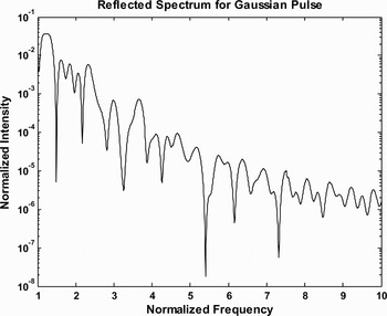
Fig. 4. Depicts the variation of the normalized harmonic intensity with normalized frequency ![]() , when the incident few-cycle (p = 2) pulse is Gaussian. The chosen parameters are: CE phase = 0, number of cycles in a pulse are p = 2, free electron density 1021 cm−3, intensity of incident laser light = 4 × 10¹⁸ W/cm2, angle of incidence = 70 degree, λ = 800 nm, center carrier frequency
, when the incident few-cycle (p = 2) pulse is Gaussian. The chosen parameters are: CE phase = 0, number of cycles in a pulse are p = 2, free electron density 1021 cm−3, intensity of incident laser light = 4 × 10¹⁸ W/cm2, angle of incidence = 70 degree, λ = 800 nm, center carrier frequency ![]() , and the thickness of metal layer l = 8 nm.
, and the thickness of metal layer l = 8 nm.
Fig. 5. (a) represents the generation of high harmonics in reflected spectrum for single cycle (p = 1) Gaussian pulse. The chosen parameters are: CE phase = 0, free electron density 1022 cm−3, intensity of incident laser light = 4 × 10¹⁸ W/cm2, angle of incidence = 45 degree, ![]() , and l = 8 nm. (b) represents the generation of high harmonics in reflected spectrum for single cycle (p = 1) hyperbolic secant pulse. The chosen parameters are: CE phase = 0, free electron density 1022 cm−3, intensity of incident laser light = 4 × 10¹⁸ W/cm2, angle of incidence = 45 degree,
, and l = 8 nm. (b) represents the generation of high harmonics in reflected spectrum for single cycle (p = 1) hyperbolic secant pulse. The chosen parameters are: CE phase = 0, free electron density 1022 cm−3, intensity of incident laser light = 4 × 10¹⁸ W/cm2, angle of incidence = 45 degree, ![]() , and l = 8 nm. (c) represents the generation of high harmonics in reflected spectrum for single cycle (p = 1) Lorentzian pulse. The chosen parameters are: CE phase = 0, free electron density 1022 cm−3, intensity of incident laser light = 4 × 10¹⁸ W/cm2, angle of incidence = 45 degree,
, and l = 8 nm. (c) represents the generation of high harmonics in reflected spectrum for single cycle (p = 1) Lorentzian pulse. The chosen parameters are: CE phase = 0, free electron density 1022 cm−3, intensity of incident laser light = 4 × 10¹⁸ W/cm2, angle of incidence = 45 degree, ![]() , and l = 8 nm.
, and l = 8 nm.
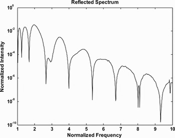
Fig. 6. Shows the variation of the normalized intensity of the harmonics in the reflected radiation caused by the incident single cycle hyperbolic secant laser pulse. The parameters are; CE phase = 1.5 radian, free electron density 1022 cm−3, intensity of incident laser light = 4 × 10¹⁸ W/cm2, angle of incidence = 50 degree, ![]() and l = 8 nm.
and l = 8 nm.
Fig. 7. Depicts the effect of variation of the CE phase on the intensity of the reflected harmonic at ω = 2ω0 caused by a single cycle Gaussian pulse. The results shown are for free electron density 1022 cm−3, intensity of incident laser light = 4 × 10¹⁸ W/cm2, angle of incidence = 45 degree, ![]() , and l = 8 nm.
, and l = 8 nm.
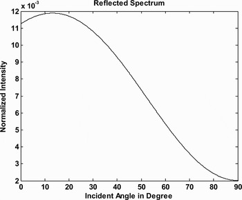
Fig. 8. Shows the variation of the intensity of the 2ω0 harmonic with angle of incidence corresponding to the incident single cycle Gaussian pulse. Numerical results are for free electron density 1022 cm−3, intensity of incident laser light = 4 × 10¹⁸ W/cm2, CE phase = 0 radian, ![]() , and l = 8 nm.
, and l = 8 nm.
5. CONCLUSION
In conclusion, this paper presents an analytical and numerical investigation of the interaction of the different laser-pulse-envelope shape with a thin plasma layer, which gives rise to HHG and Wakefield generation. Our numerical results show that the reflected radiation exhibits the presence of quasi-static “frozen-in” Wakefield in the time-domain and high harmonics of the incident laser pulse in frequency domain. The harmonic peaks are found to depend upon carrier-envelope phase difference, number of cycles, angle of incidence, and thickness of the plasma layer. The magnitude of the Wakefield is also found to depend on CEP, and angle of incidence. The Wakefield decays in a time which varies inversely to the product of the squared plasma frequency and thickness of plasma layer.
ACKNOWLEDGMENTS
Financial support from the Department of Science & Technology, New-Delhi (Government of India) is thankfully acknowledged. The authors are very-much thankful to the Referees for their valuable suggestions. The authors are thankful to Professor Naresh Dadhich, Vice-Chancellor, V. M. O. U. Kota for support, encouragement, and his keen interest in the outcome of this work. Authors are thankful to Professor N. K. Jaiman, Head, Department of Pure and Applied Physics, University of Kota, Kota for several academic discussions, support, and encouragement. Authors are thankful to Mr. Rakesh Sharma, and Professor M. K. Ghadoliya for administrative support.
APPENDIX
Derivation of Fourier Transform of Local Velocity for Lorentz Pulse-Shape
Using Eq. (3) the value of the derivative ![]() for the Lorentz pulse-shape can be obtained approximately as:
for the Lorentz pulse-shape can be obtained approximately as:
![{d{\rm \delta}_{\bot} \over d{\rm \xi}} \approx {eF_0 \over m{\rm \omega}_0} \times {\sin \left({\rm \omega}_0 {\rm \xi} + {\rm \phi} + {\rm \alpha} \right)\over \left[1 + \displaystyle\left({1.29{\rm \xi} \over {\rm \tau}} \right)^2 \right]\sqrt{1 +\displaystyle \left({{\rm \Gamma} \cos {\rm \theta} \over {\rm \omega}_0} \right)^2}}\comma \; \eqno\lpar 13\rpar](https://static.cambridge.org/binary/version/id/urn:cambridge.org:id:binary:20151021092105787-0842:S0263034610000741_eqn13.gif?pub-status=live)
where
![{\rm \alpha} = \sin^{ - 1} \left[{\displaystyle{{\rm \Gamma} \cos {\rm \theta} \over {\rm \omega}_0} \over {\sqrt{1 + \left(\displaystyle{{\rm \Gamma} \cos {\rm \theta} \over {\rm \omega}_0} \right)^2}}} \right]. \eqno\lpar 14\rpar](https://static.cambridge.org/binary/version/id/urn:cambridge.org:id:binary:20151021092105787-0842:S0263034610000741_eqn14.gif?pub-status=live)
Substituting Eq. (13) in Eq. (4) and integrating, we obtain:
![\eqalign{{{\rm \delta}_{\rm II} \over c} &\approx 2{\rm \beta} ^2 \left[\vphantom{\left. {\left.+ {2.58{\rm \xi} \over {\rm \tau} \left[1 + \left( { \textstyle1.29{\rm \xi} \over\textstyle {\rm \tau}} \right)^2 \right]} \right\}- {\sin \lpar 2A\rpar \over 4{\rm \omega}_0\left[1 + \left({\textstyle 1.29{\rm \xi} \over \textstyle {\rm \tau}} \right)^2 \right]^2}} \right]} {{\rm \tau} \over 10.32} \left\{ \vphantom{\left. {\left.+ {2.58{\rm \xi} \over {\rm \tau} \left[1 + \left( { \textstyle1.29{\rm \xi} \over\textstyle {\rm \tau}} \right)^2 \right]} \right\}- {\sin \lpar 2A\rpar \over 4{\rm \omega}_0\left[1 + \left({\textstyle 1.29{\rm \xi} \over \textstyle {\rm \tau}} \right)^2 \right]^2}} \right]}{\rm \pi} + 2\tan^{ - 1} \left({1.29{\rm \xi} \over {\rm \tau}} \right)\right. \right. \cr &\quad \left. {\left.+ {2.58{\rm \xi} \over {\rm \tau} \left[1 + \left( { \textstyle1.29{\rm \xi} \over\textstyle {\rm \tau}} \right)^2 \right]} \right\}- {\sin \lpar 2A\rpar \over 4{\rm \omega}_0\left[1 + \left({\textstyle 1.29{\rm \xi} \over \textstyle {\rm \tau}} \right)^2 \right]^2}} \right]\comma \; } \eqno\lpar 15\rpar](https://static.cambridge.org/binary/version/id/urn:cambridge.org:id:binary:20151021092105787-0842:S0263034610000741_eqn15.gif?pub-status=live)
where ![]() , and
, and
Also, using Eq. (5) and Eq. (13), we get:
![{1 \over c} {d{\rm \delta}_y \over dt} \approx {2{\rm \beta} \sin \lpar A\rpar \cos {\rm \theta} \over \left[1 + \left(\displaystyle{1.29{\rm \xi} \over {\rm \tau}} \right)^2 \right]} + {2{\rm \beta}^2 \sin^2 \lpar A\rpar \sin {\rm \theta} \over \left[1 + \left(\displaystyle{1.29{\rm \xi} \over {\rm \tau}} \right)^2 \right]^2}. \eqno\lpar 17\rpar](https://static.cambridge.org/binary/version/id/urn:cambridge.org:id:binary:20151021092105787-0842:S0263034610000741_eqn17.gif?pub-status=live)
Fourier transforming Eq. (17), we get
![\eqalign{{d{\rm \delta}_y \lpar {\rm \omega}\rpar \over dt^{\prime}} &\approx \exp \left({i{\rm \beta}^2 {\rm \omega \tau \pi} \over 5.16} \right)\times \vint_{ - \infty}^{\infty} d{\rm \xi}\ L\lpar {\rm \xi} \rpar \cr &\quad \times \exp \left[i{\rm \omega \xi} \left(1 + {{\rm \beta}^2 \over 2 \left\{1 + \left(\displaystyle{1.29{\rm \xi} \over {\rm \tau}} \right)^2 \right\}} \right)\right]\cr &\quad \times \exp \left[i{\rm \omega \beta}^2 {{\rm \tau} \over 2.58} \tan^{ - 1} \left(\displaystyle{1.29 {\rm \xi} \over {\rm \tau}} \right)\right]\comma \; } \eqno\lpar 18\rpar](https://static.cambridge.org/binary/version/id/urn:cambridge.org:id:binary:20151021092105787-0842:S0263034610000741_eqn18.gif?pub-status=live)
where
![\eqalign{{L\lpar {\rm \xi}\rpar \over c} &= \left[{2{\rm \beta} \sin \lpar A\rpar \cos {\rm \theta} \over \left\{1 + \left(\displaystyle{1.29{\rm \xi} \over {\rm \tau}} \right)^2 \right\}} + {2{\rm \beta}^2 \sin^2 \lpar A\rpar \sin {\rm \theta} \over \left\{1 + \left(\displaystyle{1.29{\rm \xi} \over {\rm \tau}} \right)^2 \right\}^2} \right]\cr &\quad \times \exp \left(- {i{\rm \omega \beta}^2 \sin \lpar 2A\rpar \over 2{\rm \omega}_0 \left\{1 + \left(\displaystyle{1.29{\rm \xi} \over {\rm \tau}} \right)^2 \right\}^2} \right).} \eqno\lpar 19\rpar](https://static.cambridge.org/binary/version/id/urn:cambridge.org:id:binary:20151021092105787-0842:S0263034610000741_eqn19.gif?pub-status=live)
Making use of the well known Bessel identity ![]() , Eq. (19) gives:
, Eq. (19) gives:
![\eqalign{{L \lpar {\rm \xi}\rpar \over c} &= \left[{2{\rm \beta} \sin \lpar A\rpar \cos {\rm \theta} \over \left\{1 + \left(\displaystyle{1.29{\rm \xi} \over {\rm \tau}} \right)^2 \right\}} + {2{\rm \beta}^2 \sin^2 \lpar A\rpar \sin {\rm \theta} \over \left\{1 + \left(\displaystyle{1.29{\rm \xi} \over {\rm \tau}} \right)^2 \right\}^2} \right]\cr &\quad \times \sum_n J_n \left({{\rm \beta}^2 {\rm \omega} \over 2{\rm \omega}_0 \left[1 + \left(\displaystyle{1.29{\rm \xi} \over {\rm \tau}} \right)^2 \right]^2} \right)\cr &\quad \times \exp \lpar \!-\! 2inA\rpar }](https://static.cambridge.org/binary/version/id/urn:cambridge.org:id:binary:20151021092105787-0842:S0263034610000741_eqnU4.gif?pub-status=live)
![\eqalignno{\Rightarrow {L\lpar {\rm \xi}\rpar \over c} &=\sum_n J_n \left({{\rm \beta}^2 {\rm \omega} \over 2{\rm \omega}_0 \left\{1 + \left(\displaystyle{1.29{\rm \xi} \over {\rm \tau}} \right)^2 \right\}^2} \right)\cr &\quad \times \bigg[ { - i{\rm \beta} \cos {\rm \theta} \over \left\{1 + \left(\displaystyle{1.29{\rm \xi} \over {\rm \tau}} \right)^2 \right\}} \left\{e^{iA\lpar 1 - 2n\rpar } - e^{iA\lpar 1 + 2n\rpar } \right\}\cr &\quad + {{\rm \beta}^2 \sin {\rm \theta} \over 2\left\{1 + \left(\displaystyle{1.29{\rm \xi} \over {\rm \tau}} \right)^2 \right\}^2} \cr &\quad \times \left\{2e^{ - i2nA} - e^{ - i2A\lpar 1 - n\rpar } - e^{ - 2iA\lpar 1 + n\rpar } \right\}\bigg] .&\lpar 20\rpar}](https://static.cambridge.org/binary/version/id/urn:cambridge.org:id:binary:20151021092105787-0842:S0263034610000741_eqn20.gif?pub-status=live)
Derivation of Fourier Transform of Local Velocity for Hyperbolic Secant Pulse-Shape
Using Eq. (3) the value of the derivative ![]() for the hyperbolic secant pulse-shape can be obtained approximately as:
for the hyperbolic secant pulse-shape can be obtained approximately as:
Substituting Eq. (21) in Eq. (4) and then integrating we obtain:
![\eqalign{{{\rm \delta}_{\rm II} \over c} &\approx 2{\rm \beta}^2 \left[{{\rm \tau} \over 3.52} \left\{\tanh \left({1.76{\rm \xi} \over {\rm \tau}} \right)- 1 \right\}\right. \cr &\quad \left. - {\left\{\sec h\left({\displaystyle1.76{\rm \xi} \over {\rm \tau}} \right)\right\}^2 \sin \lpar 2A\rpar \over 4{\rm \omega}_0} \right].} \eqno\lpar 22\rpar](https://static.cambridge.org/binary/version/id/urn:cambridge.org:id:binary:20151021092105787-0842:S0263034610000741_eqn22.gif?pub-status=live)
Substituting Eq. (21) in Eq. (5) one obtains:
Fourier transforming Eq. (23), we get
![\eqalign{{d{\rm \delta}_y \lpar {\rm \omega}\rpar \over dt^{\prime}} &\approx \exp \left(- {i{\rm \beta}^2 {\rm \omega \tau} \over 1.76} \right)\times \vint_{- \infty}^{\infty} d{\rm \xi} \ H\lpar {\rm \xi}\rpar \exp \left[i{\rm \omega \xi} \right]\cr &\quad \times \exp \left[i{\rm \omega \beta}^2 {{\rm \tau} \over 1.76} \tanh \left({1.76 {\rm \xi} \over {\rm \tau}} \right)\right]\comma \; } \eqno\lpar 24\rpar](https://static.cambridge.org/binary/version/id/urn:cambridge.org:id:binary:20151021092105787-0842:S0263034610000741_eqn24.gif?pub-status=live)
where
![\eqalign{{H \lpar {\rm \xi}\rpar \over c} &= \left[2{\rm \beta} \sec h \left({1.76{\rm \xi} \over {\rm \tau}} \right)\sin \lpar A\rpar \cos {\rm \theta} \right. \cr &\quad \left. + 2 \left\{\sec h \left({1.76{\rm \xi} \over {\rm \tau}} \right)\right\}^2 {\rm \beta}^2 \sin^2 \lpar A\rpar \sin {\rm \theta} \right]\cr &\quad \times \exp \left[-i {{\rm \omega} \over 2 {\rm \omega}_0 \beta}^2 \left\{\sec h \left({1.76{\rm \xi} \over {\rm \tau}} \right)\right\}^2 \sin \lpar 2A\rpar \right].} \eqno\lpar 25\rpar](https://static.cambridge.org/binary/version/id/urn:cambridge.org:id:binary:20151021092105787-0842:S0263034610000741_eqn25.gif?pub-status=live)
Further using Bessel identity, Eq. (25) gives:
![\eqalign{{H \lpar {\rm \xi}\rpar \over c} &= \left[2{\rm \beta} \sec h\left({1.76{\rm \xi} \over {\rm \tau}} \right)\sin \lpar A\rpar \cos {\rm \theta} \right. \cr &\quad \left. + 2\left\{\sec h\left({1.76{\rm \xi} \over {\rm \tau}} \right)\right\}^2 {\rm \beta}^2 \sin^2 \lpar A\rpar \sin {\rm \theta} \right]\cr &\quad \times \sum_n J_n \left[{\rm \beta}^2 {{\rm \omega} \over 2{\rm \omega}_0} \left\{\sec h\left({1.76{\rm \xi} \over {\rm \tau}} \right)\right\}^2 \right]\cr &\quad \times \exp \lpar \!-\! 2inA\rpar \comma \cr \Rightarrow {H \lpar {\rm \xi}\rpar \over c} &= \sum_n J_n \left[{\rm \beta}^2 {{\rm \omega} \over 2{\rm \omega}_0} \left\{\sec h\left({1.76{\rm \xi} \over {\rm \tau}} \right)\right\}^2 \right]\cr &\quad \times \left[- i{\rm \beta} \sec h\left({1.76{\rm \xi} \over {\rm \tau}} \right)\cos {\rm \theta} \right. \cr &\quad \times \left. \left\{e^{iA\lpar 1 - 2n\rpar } - e^{iA \lpar 1 + 2n\rpar } \right\}\right. \cr &\quad \left. +{{\rm \beta}^2 \over 2} \left\{\sec h \left({1.76{\rm \xi} \over {\rm \tau}} \right)\right\}^2 \sin {\rm \theta} \right. \cr & \quad \times \left. \left\{ 2e^{ - i2nA} - e^{ - i2A\lpar 1 - n\rpar } - e^{ - 2iA\lpar 1 + n\rpar} \right.\right\}\bigg].}](https://static.cambridge.org/binary/version/id/urn:cambridge.org:id:binary-alt:20160626175206-93178-mediumThumb-S0263034610000741_eqnU5.jpg?pub-status=live)
Derivation of Fourier Transform of Local Velocity for Gaussian Pulse-Shape
Using Eq. (3) the value of the derivative ![]() for the Gaussian pulse-shape can be obtained approximately as:
for the Gaussian pulse-shape can be obtained approximately as:
Substituting Eq. (26) in Eq. (5) one obtains:
Fourier transforming, we get
where ![]() , and
, and
![\eqalign{{G \lpar {\rm \xi}\rpar \over c} & = \left[2{\rm \beta} \sin \lpar A\rpar \cos {\rm \theta} \exp \left\{- \left({1.17{\rm \xi} \over {\rm \tau}} \right)^2 \right\}\right. \cr &\quad \left. + 2{\rm \beta}^2 \sin^2 \lpar A\rpar \sin {\rm \theta} \exp \left\{- 2\left({1.17{\rm \xi} \over {\rm \tau}} \right)^2 \right\}\right]\cr &\quad \times \exp \left[- i {{\rm \omega} \over 2{\rm \omega}_0} \exp \left\{- 2\left({1.17{\rm \xi} \over {\rm \tau}} \right)^2 \right\}{\rm \beta}^2 \sin \lpar 2A\rpar \right].} \eqno\lpar 29\rpar](https://static.cambridge.org/binary/version/id/urn:cambridge.org:id:binary:20151021092105787-0842:S0263034610000741_eqn29.gif?pub-status=live)
Using the Bessel identity, Eq. (29) gives:
![\eqalign{{G \lpar {\rm \xi}\rpar \over c} & = \sum_n J_n \left[{\rm \beta}^2 {{\rm \omega} \over 2{\rm \omega}_0} \exp \left\{- 2 \left({1.17{\rm \xi} \over {\rm \tau}} \right)^2 \right\}\right]\cr &\quad \times \bigg[- i{\rm \beta} \cos {\rm \theta} \left\{e^{iA\lpar 1 - 2n\rpar } - e^{iA\lpar 1 + 2n\rpar } \right\} . \times \exp \left\{- \left({1.17{\rm \xi} \over {\rm \tau}} \right)^2 \right\} \cr &\quad + {{\rm \beta}^2 \over 2} \sin {\rm \theta} \left\{2e^{ - i2nA} - e^{ - i2A\lpar 1 - n\rpar } - e^{- 2iA\lpar 1 + n\rpar} \right\} \cr &\quad \times \exp \left\{- 2\left({1.17{\rm \xi} \over {\rm \tau}} \right)^2 \right\}\bigg].}](https://static.cambridge.org/binary/version/id/urn:cambridge.org:id:binary:20151021092105787-0842:S0263034610000741_eqnU6.gif?pub-status=live)


