


1. Introduction
Taylor–Couette flow (TCF), which considers the closed motion of fluid lying between concentric cylinders driven by the rotation of these cylinders about their shared axis, has long been serving as a canonical problem from which to study the mechanisms of the transition to turbulence. TCF is governed by three parameters that quantify the effects of rotation, shear and curvature of the walls, with anticyclonic rotation (i.e. rotation for which the rotation vector points in the opposite direction to the vorticity of the base flow), which destabilises the flow, producing a rich structure of transitionary flows that include the streamwise-independent Taylor vortices, wavy-vortex flows (WVFs), twisted vortex flows and so on, while the stabilising cyclonic rotation regime permits flow regimes that include laminar–turbulent coexistence and featureless turbulence. An early experimental overview of these flow regimes is provided by Cole (Reference Cole1976) and Anderek, Liu & Swinney (Reference Anderek, Liu and Swinney1986), while reviews of this flow are provided by Koschmieder (Reference Koschmieder1992), Fardin, Perge & Taberlet (Reference Fardin, Perge and Taberlet2014) and Grossman, Lohse & Sun (Reference Grossman, Lohse and Sun2016).
The present study considers the related problem of rotating plane Couette flow (RPCF), which considers channel flow driven by the in-plane motion of the parallel channel walls, subject to a system rotation about a spanwise axis. Although RPCF, in contrast to TCF, is an open flow that is governed instead by two parameters expressing the effects of system rotation and shear, RPCF exhibits many similarities in the observed flow structures and transitions with TCF (Mullin Reference Mullin2010; Brauckmann, Salewski & Eckhardt Reference Brauckmann, Salewski and Eckhardt2016). A number of experimental studies have explored the parameter space, and have confirmed the richness of the observable flow types (Tillmark & Alfredsson Reference Tillmark and Alfredsson1996; Hiwatashi et al. Reference Hiwatashi, Alfredsson, Tillmark and Nagata2007; Tsukahara, Tillmark & Alfredsson Reference Tsukahara, Tillmark and Alfredsson2010; Suryadi, Segalini & Alfredsson Reference Suryadi, Segalini and Alfredsson2014; Kawata & Alfredsson Reference Kawata and Alfredsson2016a,Reference Kawata and Alfredssonb).
A good overview is provided by figures 2 and 3 of Tsukahara et al. (Reference Tsukahara, Tillmark and Alfredsson2010), who map out flow regimes including, in the anticyclonic case, two-dimensional roll cells (2dRCs), analogous to Taylor vortices, WVF, turbulence that includes roll-cell structures and turbulence embedded within roll-cell structures. In the cyclonic case, flow regimes include turbulent spots, regions of laminar–turbulent coexistence and featureless turbulence. A comparison of these maps with the corresponding map for TCF provided by Anderek et al. (Reference Anderek, Liu and Swinney1986) in their figure 1 emphasises the strong similarities between these two flows.
Numerical and theoretical studies of transitionary RPCF flows have included the description of the bifurcation from the 2dRC to WVF (Nagata Reference Nagata1986, Reference Nagata1988), the confirmation of the stability of the WVF in a certain parameter range (Nagata Reference Nagata1998), the description of twist vortices (Weisshaar, Busse & Nagata Reference Weisshaar, Busse and Nagata1991), a two-layered ribbon solution (Nagata Reference Nagata2013), braided vortex structures and other tertiary flow types (Daly et al. Reference Daly, Schneider, Schlatter and Peake2014).
More recently, research on RPCF has extended from studies of the different bifurcations and flow patterns to include investigations of the turbulent regime, with detailed analyses of physical quantities such as momentum transport, torque and energy dissipation, including the numerical studies conducted by Faisst & Eckhardt (Reference Faisst and Eckhardt2000), Dubrulle et al. (Reference Dubrulle, Dauchot, Daviaud, Longaretti, Richard and Zahn2005), Eckhardt, Grossmann & Lohse (Reference Eckhardt, Grossmann and Lohse2007a), Eckhardt, Grossmann & Lohse (Reference Eckhardt, Grossmann and Lohse2007b), Salewski & Eckhardt (Reference Salewski and Eckhardt2015) and Brauckmann et al. (Reference Brauckmann, Salewski and Eckhardt2016). These studies also investigated the mechanisms that exist for large enough Reynolds number, for momentum transport in the anticyclonic range with changing rotation number, with these findings largely supported by the later experimental observations of Kawata & Alfredsson (Reference Kawata and Alfredsson2019). Similar results for the angular momentum transfer in TCF were found both in the numerical simulations of Brauckmann et al. (Reference Brauckmann, Salewski and Eckhardt2016) and in the experimental observations of Tokgoz et al. (Reference Tokgoz, Elsinga, Delfos and Westerweel2020).
Other recent studies have considered the multiplicity of the turbulent state, with Xia et al. (Reference Xia, Shi, Cai, Wan and Chen2019) finding two distinct flows for the same parameters, one characterised by three pairs of roll cells and the other characterised by two pairs of roll cells. These flows were later found to be connected by a hysteresis loop in the changing rotation number (Huang et al. Reference Huang, Xia, Wan, Shi and Chen2019).
In the present study, in contrast to the topics considered in these turbulent studies, we reconsider the opposite end of transition analysis, focusing on the fluid behaviour in the vicinity of where the instability of the laminar basic state sets in. It is widely accepted that a streamwise-independent flow with a 2dRC structure appears first as the secondary flow when the laminar flow becomes unstable. The bifurcation is known theoretically to take place at the rotation number  $\bar {\varOmega }=1.079\times 10^{2}$ for the spanwise wavenumber
  $\beta = 1.5585$ and the Reynolds number
  $Re = 100$ (the definitions of
  $\bar \varOmega$ and
  $Re$ are given in (2.3a–c)). This roll-cell secondary flow then, in turn, loses stability to a bifurcating wavy-vortex tertiary flow.
However, there are certain problems with the explanation of the transition from the laminar flow as described previously. For example, the experimental observation by Hiwatashi et al. (Reference Hiwatashi, Alfredsson, Tillmark and Nagata2007) detected an oscillatory flow pattern that appears and vanishes repeatedly with a period of a few minutes for  $Re = 101$ and
  $\varOmega \equiv Re \bar \varOmega = 1.73$.
Furthermore, flow patterns of the 2dRC observed by Tsukahara et al. (Reference Tsukahara, Tillmark and Alfredsson2010) and Kawata & Alfredsson (Reference Kawata and Alfredsson2016a) are not strictly aligned in the streamwise direction, but are slightly tilted (see their figures 7(a) and 3(a), respectively).
In the following, we show that there exist no stable 2dRCs, at least in the small region of  $\varOmega$ adjacent to its critical value
  $\varOmega _C = 1.079$, and that the newly found flows presented in this study, tilted-vortex flow and periodic-vortex flow, can explain the appearance of complicated flow structures observed by the above experiments.
The basic equations are introduced in § 2, followed by the description of the numerical schemes to be used in § 3. The results of the bifurcation analysis are provided in § 4, where, in particular, § 4.5 is devoted to the analysis of tilted-vortex flow. The periodic-vortex flow is described in § 5. Finally, the present study is concluded in the summary in § 6.
2. Basic equations
We consider motion of a fluid with the density  $\rho ^*$ and the kinematic viscosity
  $\nu ^*$ between two parallel plates of infinite extent separated by a distance
  $d^*$. We denote the unit vectors in the streamwise
  $(x^*)$, spanwise
  $(y^*)$ and the wall-normal
  $(z^*)$ directions by
  $\boldsymbol {i}$,
  $\boldsymbol {j}$ and
  $\boldsymbol {k}$, respectively. The plates are in an in-plane translational motion,
  $\pm U_0^*$ at
  $z^* = \mp d^*$, with the whole system subject to a rotation
  $\varOmega _0^*$ about a spanwise axis (see figure 1).

Figure 1. Physical configuration.
Following Nagata (Reference Nagata2013), we write the basic equations in the dimensionless form as
 \begin{gather} \boldsymbol{\nabla} \boldsymbol{\cdot} {\boldsymbol{u}} = 0, \end{gather}
 \begin{gather}\partial_t {\boldsymbol{u}} + ({\boldsymbol{U}}_B \boldsymbol{\cdot} \boldsymbol{\nabla}) {\boldsymbol{u}} + ({\boldsymbol{u}} \boldsymbol{\cdot} \boldsymbol{\nabla}) {\boldsymbol{U}}_B + ({\boldsymbol{u}} \cdot \boldsymbol{\nabla}) {\boldsymbol{u}} + \bar\varOmega {\boldsymbol{j}}\times {\boldsymbol{u}} ={-}\boldsymbol{\nabla} p + \frac{1}{Re}\nabla^2{\boldsymbol{u}}, \end{gather}
where  ${\boldsymbol {u}} = {\boldsymbol {U}_B(z)} + \tilde {\boldsymbol {u}}$ is the total velocity composed of the laminar basic velocity
  ${\boldsymbol {U}_B(z)}$ and the superposed disturbance velocity
  $\tilde {\boldsymbol {u}}$. The basic state velocity is given by
  ${\boldsymbol {U}_B(z)} = U_B(z){\boldsymbol {i}} = -z {\boldsymbol {i}}$, where
  $z$ varies from
  $-$1 to 1. The parameters that control the system are the Reynolds number,
  $Re$, and the rotation number,
  $\bar {\varOmega }$, defined by
 \begin{equation} Re = \frac{U_0^* d^*}{\nu^*}, \quad \bar{\varOmega} = \frac{2 \varOmega_0^* d^*}{U_0^*}, \quad \left( \varOmega=Re \bar{\varOmega}=\frac{2 \varOmega_0^* {d^*}^2}{\nu^*} \right).\end{equation}
 For convenience, we decompose the velocity disturbance  $\tilde {\boldsymbol {u}}$ into a mean-flow modification with components
  $\check {U}(z){\boldsymbol {i}}$ in the streamwise direction and
  $\check {V}(z){\boldsymbol {j}}$ in the spanwise direction, and a spatially periodic
  $\check {\boldsymbol {u}}$. We introduce the general expression for the solenoidal vector field
  $\check {\boldsymbol {u}}$, using the poloidal and toroidal functions,
  $\phi$ and
  $\psi$, respectively, as
 \begin{equation} \check{\boldsymbol{u}}= \boldsymbol{\nabla}\times(\boldsymbol{\nabla}\times {\boldsymbol{k}}\phi) + \boldsymbol{\nabla}\times {\boldsymbol{k}}\psi =(\partial^2_{xz}\phi+ \partial_y \psi, \partial^2_{yz}\phi - \partial_x \psi, -\varDelta_2 \phi ), \end{equation}
where  $\varDelta _2 = \partial ^2_{xx} + \partial ^2_{yy}$. Note that with this decomposition the continuity equation is satisfied automatically.
Applying the operations  ${\boldsymbol {k}}\boldsymbol {\cdot }\boldsymbol {\nabla }\times \boldsymbol {\nabla }\times$ and
  ${\boldsymbol {k}}\boldsymbol {\cdot }\boldsymbol {\nabla }\times$ to equation (2.2) yields the equations
 \begin{align} \partial_t \nabla^2\varDelta_2\phi &= ( \nabla^4 +(U_B+\check{U})''\partial_x + \check{V}'' \partial_y - (U_B+\check{U} ) \partial_x \nabla^2 -\check{V}\partial_y \nabla^2 ) \varDelta_2 \phi \nonumber\\ &\quad - {\varOmega}\partial_y \varDelta_2\psi -{\boldsymbol{k}}\boldsymbol{\cdot}\boldsymbol{\nabla}\times\boldsymbol{\nabla}\times[(\check{\boldsymbol{u}}\boldsymbol{\cdot}\boldsymbol{\nabla})\check{\boldsymbol{u}}],\end{align}
 \begin{align} \partial_t \varDelta_2\psi &= ( \nabla^2 - (U_B+\check{U})\partial_x - \check{V}\partial_y ) \varDelta_2 \psi \nonumber\\ &\quad + ( (U_B+\check{U})'\partial_y + {\varOmega}\partial_y - \check{V}'\partial_x )\varDelta_2\phi +{\boldsymbol{k}}\boldsymbol{\cdot}\boldsymbol{\nabla}\times[(\check{\boldsymbol{u}}\boldsymbol{\cdot}\boldsymbol{\nabla})\check{\boldsymbol{u}}], \end{align}
respectively, where we also rescaled  $(\partial _t, U_B, \tilde {\boldsymbol {u}}) \rightarrow ({1}/{Re}) (\partial _t, U_B, \tilde {\boldsymbol {u}})$ for convenience.
Here,  $U_B(z)=-Re z$ and the prime
  $(')$ denotes differentiation with respect to
  $z$.
$z$.
The nonlinear interaction terms  ${\boldsymbol {k}}\boldsymbol {\cdot }\boldsymbol {\nabla }\times \boldsymbol {\nabla }\times [(\check {\boldsymbol {u}}\boldsymbol {\cdot }\boldsymbol {\nabla })\check {\boldsymbol {u}}]$ in (2.5) and
  ${\boldsymbol {k}}\boldsymbol {\cdot }\boldsymbol {\nabla }\times [(\check {\boldsymbol {u}}\boldsymbol {\cdot }\boldsymbol {\nabla })\check {\boldsymbol {u}}]$ in (2.6) are listed in the Appendix of Masuda, Fukuda & Nagata (Reference Masuda, Fukuda and Nagata2008).
Averaging the  $x$- and the
  $y$-component of (2.2) in
  $xy$-space further yields the mean flow relations
 \begin{gather} \partial_t \check{U}= \check{U}'' + \partial_z \overline{ \varDelta_2 \phi ( \partial^2_{xz}\phi + \partial_y \psi ) }, \end{gather}
 \begin{gather}\partial_t \check{V}= \check{V}'' + \partial_z \overline{ \varDelta_2 \phi ( \partial^2_{yz}\phi - \partial_x \psi ) }, \end{gather}
respectively. The no-slip boundary conditions become
 \begin{equation} \phi=\partial_z \phi=\psi=\check{U}=\check{V}= 0 \quad \mbox{at } z={\pm} 1. \end{equation}
It is known that streamwise-independent flows, as a special case solution, are controlled by a single parameter, the Taylor number, defined by
 \begin{equation} Ta=\varOmega(Re-\varOmega), \end{equation}
(see, for example, Nagata Reference Nagata2013).
In the following sections, we seek steady solutions by the Newton–Raphson iterative method, and also seek time-dependent solutions by numerical time integration, where we choose the momentum transport  $M_T$ at
  $z=-1$ as a nonlinear measure of these solutions
 \begin{equation} M_T=\left.\frac{\mbox{d}U}{\mbox{d}z} \right|_{z={-}1}, \end{equation}
where  $U=U_B + {\check U}$.
Once a steady solution is obtained, we can examine its stability by calculating the growth rate of infinitesimal perturbations  $\tilde {\phi }$ and
  $\tilde {\psi }$, which are superposed on
  $\phi$ and
  $\psi$, respectively, in (2.5) and (2.6). The equations to be solved for
  $\tilde {\phi }$ and
  $\tilde {\psi }$ are obtained after linearisation with respect to
  $\tilde {\phi }$ and
  $\tilde {\psi }$ as
 \begin{align} \partial_t \nabla^2\varDelta_2\tilde{\phi} &= ( \nabla^4 +(U_B+\check{U})''\partial_x + \check{V}'' \partial_y - (U_B+\check{U} ) \partial_x \nabla^2 -\check{V}\partial_y \nabla^2 ) \varDelta_2 \tilde{\phi} \nonumber\\ &\quad - {\varOmega}\partial_y \varDelta_2\tilde{\psi} -{\boldsymbol{k}}\boldsymbol{\cdot}\boldsymbol{\nabla}\times\boldsymbol{\nabla}\times[(\check{\boldsymbol{u}}\boldsymbol{\cdot}\boldsymbol{\nabla})\tilde{\boldsymbol{u}}] -{\boldsymbol{k}}\boldsymbol{\cdot}\boldsymbol{\nabla}\times\boldsymbol{\nabla}\times[(\tilde{\boldsymbol{u}}\boldsymbol{\cdot}\boldsymbol{\nabla})\check{\boldsymbol{u}}], \end{align}
 \begin{align} \partial_t \varDelta_2 \tilde{\psi} &= ( \nabla^2 - (U_B+\check{U})\partial_x - \check{V}\partial_y ) \varDelta_2 \tilde{\psi} + ( (U_B+\check{U})'\partial_y + {\varOmega}\partial_y - \check{V}'\partial_x )\varDelta_2\tilde{\phi} \nonumber\\ & \quad + {\boldsymbol{k}}\boldsymbol{\cdot}\boldsymbol{\nabla}\times[(\check{\boldsymbol{u}}\boldsymbol{\cdot}\boldsymbol{\nabla})\tilde{\boldsymbol{u}}] + {\boldsymbol{k}}\boldsymbol{\cdot}\boldsymbol{\nabla}\times[(\tilde{\boldsymbol{u}}\boldsymbol{\cdot}\boldsymbol{\nabla})\check{\boldsymbol{u}}]], \end{align}
with the boundary conditions
 \begin{equation} \tilde\phi=\partial_z \tilde\phi=\tilde\psi= 0 \mbox{ at } z={\pm} 1.\end{equation}
3. Numerical analyses
3.1. Numerical schemes
It is of our interest to find nonlinear solutions which are expected to bifurcate as  $\varOmega$ is increased for a fixed value of the Reynolds number. Finite-amplitude solutions,
  $\phi$,
  $\psi$,
  $\check U$ and
  $\check V$, satisfying (2.5)–(2.8) subject to the boundary conditions (2.9), are expanded as
 \begin{gather} \phi(x, y, z, t) =\sum_{l=0}^{L} \sum_{\substack{m={-}M \\ (m,n) \neq (0,0)} }^{M } \sum_{n={-}N}^{N} a_{lmn}(t) \exp[\textrm{i}m \alpha x+\textrm{i}n\beta y] f_l (z), \end{gather}
 \begin{gather}\psi(x, y, z, t) =\sum_{l=0}^{L} \sum_{\substack{m={-}M \\ (m,n)\neq (0,0)} }^{M } \sum_{n={-}N}^{N} b_{lmn}(t) \exp[\textrm{i}m \alpha x+\textrm{i}n\beta y] g_l (z), \end{gather}
 \begin{gather}{\check U}(z,t) =\sum_{l=0}^{L} c_{\ell}(t) g_l (z), \end{gather}
 \begin{gather}{\check V}(z,t) =\sum_{l=0}^{L} d_{\ell}(t) g_l (z), \end{gather}
at the truncation level  $(L, M, N)$, where
  $\alpha$ and
  $\beta$ are the wavenumbers in the streamwise and the spanwise directions, respectively, and the modified Chebyshev polynomials
  $f_\ell (z) = (1-z^2)^2 T_\ell (z)$ and
  $g_\ell (z) = (1-z)^2 T_\ell (z)$ are introduced so as to satisfy the boundary conditions automatically, where
  $T_\ell (z)$ represents the
  $\ell$th Chebyshev polynomial of the first kind.
It is found that not all the disturbance components are involved in forming a particular solution, but a limited number of the components satisfying a certain class of symmetry, depending on the spatial flow structure, constitutes a nonlinearly interacting closed set. The number of disturbance components to be determined can be reduced by incorporating such symmetries in the numerical codes.
We substitute into (2.5)–(2.8) for a solution of the form (3.1)–(3.4). We multiply (2.5) and (2.6) by  $\exp [-\textrm {i}(m_0\alpha x + n_0\beta y)]$ and take their
  $(x, y)$-average. Then, all the equations are evaluated at the internal collocation points
 \begin{equation} z_j = \cos \frac{j {\rm \pi}}{L+2}, \quad j=1,\ldots, L+1, \end{equation}
in order to complete the discretisation procedure. By allowing  $m_0$,
  $n_0$ and
  $\ell _0$ to run through all permissible values, we get the following system of algebraic equations for each of the time-dependent amplitudes,
  $a_{\ell m n}$,
  $b_{\ell m n}$,
  $c_\ell$ and
  $d_\ell$,
 \begin{equation} C_{ij} \dot{x}_j = A_{ij} x_j + B_{ijk} x_j x_k, \quad x_j \in \{ a_{lmn}, b_{lmn}, c_\ell, d_\ell \}, \end{equation}
where a dot denotes the time derivative. The elements of  $C_{ij}$ and
  $A_{ij}$ are obtained by collecting coefficients for
  $a_{\ell _1 m_1 n_1}$,
  $b_{\ell _1 m_1 n_1}$,
  $c_{\ell _1}$ and
  $d_{\ell _1}$ with
  $m_1 = m_0$ and
  $n_1 = n_0$ from the linear terms, while those of
  $B_{ijk}$ are obtained by collecting coefficients for
  $a_{\ell _1 m_1 n_1}, b_{\ell _1 m_1 n_1}, c_{\ell _1}$ and
  $d_{\ell _1}$ and
  $a_{\ell _2 m_2 n_2}, b_{\ell _2 m_2 n_2}, c_{\ell _2}$ and
  $d_{\ell _2}$ satisfying
  $m_1 + m_2 = m_0$ and
  $n_1 + n_2 = n_0$ from the nonlinear terms.
For a steady-state case, the above set of equations becomes a system of nonlinear algebraic equations,
 \begin{equation} A_{ij} x_j + B_{ijk} x_j x_k = 0, \quad x_j \in \{a_{lmn}, b_{lmn}, c_\ell, d_\ell \}, \end{equation}
which are solved by the Newton–Raphson iterative method, where the number of unknowns of this system of equations may be reduced by consideration of the symmetries of the bifurcating flows as discussed previously.
Once the steady-state solution is obtained, its stability is analysed by calculating the growth rate  $\sigma$ of superimposed infinitesimal perturbation
  $\tilde \phi$ and
  $\tilde \psi$ on
  $\phi$ and
  $\psi$, respectively,
 \begin{gather} \tilde{\phi}(x, y, z, t) =\sum_{l=0}^{L} \sum_{m={-}M}^{M} \sum_{n={-}N}^{N} \tilde{a}_{lmn} \exp[\textrm{i}m \alpha x+\textrm{i}n\beta y] \exp (\textrm{i}dx + \textrm{i}by + \sigma t) f_l (z), \end{gather}
 \begin{gather}\tilde{\psi}(x, y, z, t) =\sum_{l=0}^{L} \sum_{m={-}M}^{M} \sum_{n={-}N}^{N} \tilde{b}_{lmn} \exp[\textrm{i}m \alpha x+\textrm{i}n\beta y] \exp (\textrm{i}dx + \textrm{i}by + \sigma t) g_l (z), \end{gather}
By Floquet theory, the perturbations have, in addition to the same wavenumbers,  $\alpha$ and
  $\beta$, as the steady state, an extra wavenumber dependency
  $(d, b)$ in the streamwise and spanwise directions, respectively. In contrast to the expressions in (3.1) and (3.2), the case
  $(m,n)=(0,0)$ is not excluded in (3.8) and (3.9). This case covers the equations for stability of the mean flow distortions, provided
  $(d,b)\neq (0,0)$.
Substitution of (3.8) and (3.9) into (2.12) and (2.13) followed by the  $(x,y)$-averaging and the evaluation at the collocation points (3.5) yields the system
 \begin{equation} C_{ij} \dot{\tilde x}_j + D_{ij} {\tilde x}_j + E_{ijk} x_j \tilde{x}_k + F_{ijk} {\tilde x}_j x_k = 0, \quad \tilde{x}_j \in \{ \tilde{a}_{lmn}, \tilde{b}_{lmn} \}, \end{equation}
which is reduced to an eigenvalue problem of the form
 \begin{equation} \sigma G_{ij} {\tilde x}_j = H_{ij} {\tilde x}_j, \quad \tilde{x}_j \in \{ \tilde{a}_{lmn}, \tilde{b}_{lmn} \}.\end{equation}
The matrices  $D_{ij}$,
  $E_{ij}$ and
  $F_{ij}$ are determined in a similar way as in the nonlinear case. The eigenvalue
  $\sigma$ is solved numerically by using the Lapack routine ZGGEV, which uses the QZ algorithm.
We also integrate (3.6) numerically in time to follow the time evolution of the flow, where two explicit methods, Euler's method and the fourth-order Runge–Kutta method, have been used to perform the time marching. The inversion of the constant matrix  $C_{ij}$ in (3.6) is necessary only once at the initial time step. The numerical code used to follow the time evolution is consistent with that used to obtain the steady-state solutions, that is, the evaluation of the right-hand side of (3.6) at each time step is carried out using the same subroutines as used for the steady-state solutions (3.7). The only difference in subroutines is that the symmetry imposed for the Newton iterative calculation of the steady-state solutions is removed for the time-evolution scheme, in order to allow arbitrary disturbance components to take part in the time-developing process. The converged steady-state solutions, obtained separately without imposing symmetry, are used to provide the initial conditions for the time evolution code, with the simulations then marching forward in time without imposing any symmetry conditions on the flow.
3.2. Convergence check
The convergence of the WVF solution, to be discussed in § 4.2, with respect to the truncation levels is listed in table 1.
Table 1. Convergence of the momentum transport  $M_T$ at
  $z=-1$ for WVF with respect to the truncation level
  $(L, M, N)$ for parameters
  $Re= 100$,
  $\varOmega =1.5$ and
  $(\alpha ,\beta )=(0.1,1.5585).$

As described previously, the Newton–Raphson iterative method and the time-evolution scheme are constructed so as to be consistent to each other, i.e. the solutions are expanded in the same manner with the same truncation level so that they can exchange data directly. In the following,  $(L, M, N)=(5,4,4)$ is selected. Although one might think that this level is rather low, we believe it turns out to be sufficient for the purpose of explaining the bifurcation structure of vortex flows that take place in the parameter region which is close to where the first instability of the basic laminar state sets in. In fact, selected calculations with higher resolution, though not such a systematic study as the present study, indicated that there is only a small numerical correction to the results (see (Nagata, Song & Wall Reference Nagata, Song and Wall2019) and the caption of table 6 later).
4. Bifurcation analysis
It is known that the basic laminar state of RPCF loses its stability at the critical Taylor number  $Ta_c^{(1)}=106.735$, against a streamwise-independent perturbation with the spanwise wavenumber
  $\beta _c^{(1)}=1.5585$. A second critical state occurs at
  $Ta_c^{(2)}=1100.650$ with
  $\beta _c^{(2)}=2.6823$. As a result, streamwise-independent flows, Taylor-vortex flow type I (TV
 $_1$) and type II (TV
 $_2$), bifurcate from the above critical Taylor numbers. The disturbance components forming TV
 $_1$ and TV
 $_2$ are listed in table 2.
Table 2. Symmetry of the streamwise-independent flows, TV $_1$ and TV
 $_2$. Here,
  $m^+$,
  $n^+$ denote odd integers whereas
  $m^{++}$,
  $n^{++}$ denote even integers. The functions
  $F_s (z)$ and
  $F_a (z)$ represent symmetric and anti-symmetric functions in
  $z$, respectively. Note
  $n$ takes both odd and even integers for TV
 $_2$.
$_2$.

Nagata (Reference Nagata2013) showed that when the Reynolds number  $Re$ is fixed at 160, three-dimensional (3-D) steady flows, WVF and 3-D ribbon bifurcate from the solution branches for TV
 $_1$ for
  $\beta =1.5$ at
  $\varOmega = 0.98$ and TV
 $_2$ for
  $\beta =3.0$ at
  $\varOmega = 8.32$, respectively, where the streamwise wavenumber
  $\alpha =0.9$ is chosen (see figure 3 of Nagata Reference Nagata2013). It is found that when
  $\alpha$ is decreased the bifurcation structure described previously changes slightly as shown in § 4.1: the bifurcation point of the ribbon approaches the bifurcation point of TV
 $_2$, and then slides to a smaller
  $\varOmega$ so that the ribbon solution then bifurcates directly from the basic state.
In the following, we fix the Reynolds number at  $Re=100$ in order to make a direct comparison possible with the experimental observations of Kawata & Alfredsson (Reference Kawata and Alfredsson2016a). In addition, we rename TV
 $_1$ as the 2dRC structure following Kawata & Alfredsson (Reference Kawata and Alfredsson2016a).
4.1. Stability of the basic laminar state and the bifurcations of 2dRC and 3-D ribbon
We start by considering the stability of the basic laminar state. To do this, all nonlinear amplitudes,  $a_{\ell m n}, b_{\ell m n}, c_\ell , d_\ell$ and the wavenumbers,
  $\alpha , \beta$, are set to zero in (3.10), and we solve for the eigenvalue
  $\sigma$ in (3.11), where the matrix
  $G_{ij}$ is a function of
  $Re, \varOmega , d,b$ in this subsection. The basic state is found to first lose stability at
  $Ta_c^{(1)}=\varOmega (Re-\varOmega ) = 106.735$, which for
  $Re=100$ corresponds to
  $\varOmega = 1.079$, to a perturbation with
  $(d,b)= (0.0, 1.5585)$. The 2dRC flow bifurcates from this point with wavenumbers,
  $(\alpha , \beta )= (0.0, 1.5585)$ as shown in figure 2(a,b). Also shown in these figures is the growth rate
  $\sigma$ of perturbation with
  $(d,b)= (0.1, 1.5585)$ which crosses zero at
  $\varOmega = 1.408$, and the branch of 3-D ribbon with
  $(\alpha ,\beta )= (0.1, 1.5585)$ which bifurcates from this value of
  $\varOmega$. It is found that the imaginary part of the eigenvalues responsible for the bifurcation of both 2dRC and 3-D ribbon is zero.

Figure 2. (a) Linear stability of the basic flow: the growth rate  $\sigma$ of streamwise-independent perturbations with
  $(d,b)=(0.0,1.5585)$ (thick curve) and 3-D perturbations with
  $(d,b)=(0.1,1.5585)$ (thin curve). (b) The bifurcation of 2dRC with
  $(\alpha ,\beta )= (0.0, 1.5585)$ (thick curve) and 3-D ribbon with
  $(\alpha , \beta )= (0.1, 1.5585)$ (thin curve). Note here the value
  $M_T=-100$ corresponds to the basic flow.
It is found that only a subset of all the possible amplitude components are involved in forming the 3-D ribbon solution. Table 3 lists these components.
Table 3. Symmetry of 3-D ribbon flow. Same notation as table 2 for  $m^+$,
  $n^+$,
  $m^{++}$,
  $n^{++}$ and
  $F_s (z)$,
  $F_a (z)$. Note this set includes the one for TV
 $_2$, when only
  $m^{++}=0$ is taken into account and
  $\beta$ is halved,
  $\tilde \beta = \beta /2$:
  $\check u: \cos (n\tilde {\beta } y) F_a(z)$,
  $\check v: \sin (n\tilde {\beta } y) F_s(z)$,
  $\check w: \cos (n\tilde {\beta } y) F_a(z)$, where
  $n$ takes both odd and even integers.

This is the simplest set of linearly and nonlinearly interacting 3-D components that can be reduced from (2.2) for which the laminar basic flow  $\boldsymbol {U}_B (z)$ is anti-symmetric in
  $z$. This set possesses the highest degree of symmetry possible in 3-D RPCF (see Nagata Reference Nagata2013). The shift-rotation symmetry,
  $\boldsymbol {\varOmega }$,
 \begin{equation} \boldsymbol{\varOmega} : [u,v,w](x,y,z)= [{-}u, v, -w]({-}x, y+{\rm \pi} /\beta, -z),\end{equation}
the shift-reflection symmetry,  $\boldsymbol {S}$,
 \begin{equation} \boldsymbol{S} : [u,v,w](x,y,z)= [u, -v, w](x+{\rm \pi} /\alpha, -y+{\rm \pi} /\beta, z), \end{equation}
and the mirror symmetry,  $\boldsymbol {Z}_y$, with respect to the plane
  $y=0$,
 \begin{equation} \boldsymbol{Z}_y : [u,v,w](x,y,z)= [u, -v, w](x, -y, z). \end{equation}
4.2. Stability of 2dRC and the bifurcation of WVF
The stability of the 2dRC obtained in the previous subsection with  $(\alpha , \beta )= (0.0, 1.5585)$ is analysed by superimposing a general form of infinitesimal perturbation. Figure 3(a) shows the growth rates
  $\sigma$ of perturbations for various values of
  $d$ ranging from 0.01 to 1.0, with fixed
  $b=0$, against
  $\varOmega$. The 2dRC is stable to a perturbation with
  $(d, 0.0)$ in the interval from
  $\varOmega = 1.079$, i.e. the bifurcation point of 2dRC, to the point where the particular curve with this value of
  $d$ crosses
  $\sigma =0$, and becomes unstable above it. For instance, in the case of
  $d=0.1$, this value of
  $\varOmega$ where the stability change takes place at
  $\varOmega = 1.244$. Also shown in the figure are the two dashed curves, which correspond to the growth rate of perturbations with
  $(d,b)=(0.0, 1.5585)$ and
  $(d,b)=(0.1, 1.5585)$ superposed on the basic state (see figure 2a). It is seen that these two growth rates of perturbations superposed on the basic flow when
  $\varOmega =1.079$ (vertical dotted line) coincide with the growth rates of perturbations superposed on the 2dRC,
  $(d, b)=(d,0.0)$ with
  $d\rightarrow 0$ and
  $(d, b)=(0.1, 0.0)$, respectively, in the limit as 2dRC approaches its bifurcation point, because the amplitude of 2dRC vanishes there (i.e. the 2dRC solution approaches the basic flow in this limit).

Figure 3. (a) The growth rate  $\sigma$ of perturbations with
  $(d, 0.0)$ superposed on 2dRC, where the values of
  $d$ are indicated in the figure (thick curves). The growth rate
  $\sigma$ of perturbations with
  $(d,b)=(0.0,1.5585)$ and
  $(d,b)=(0.1,1.5585)$ superposed on the basic state (thin dashed curves) (see figure 2). (b) The branch of WVF with
  $(\alpha , \beta )=(0.1, 1.5585)$ (dashed curve) connecting the branches of 2dRC with
  $(\alpha ,\beta )=(0.0, 1.5585)$ (thick curve) and 3-D ribbon with
  $(\alpha , \beta )=(0.1, 1.5585)$ (thin curve).
It can thus be seen that the point at which 2dRC loses stability approaches the point of bifurcation of this flow from the basic state in the limit as  $d$ is decreased towards zero. (Daly et al. (Reference Daly, Schneider, Schlatter and Peake2014) analysed the stability of 2dRCs and found wavy-vortex instability in the region of
  $0 \leq Ro \leq 0.13$ and
  $0 \leq \alpha \leq 0.8$ for
  $Re=100$ and
  $\beta =1.5$ (see their figure 6b). Their
  $\alpha$ and
  $Ro$ correspond to our
  $d$ and
  $\varOmega /Re$. However, they did not pursue further the instability at
  $d\simeq 0$.) This indicates that 2dRC is unstable from its bifurcation point to a perturbation in the long limit of streamwise wavelength, leaving no stable interval on the 2dRC branch, at least in the vicinity of its bifurcation point. It is natural then to ask what kind of flow state is expected, noting that Kawata & Alfredsson (Reference Kawata and Alfredsson2016a) described observing straight streamwise-oriented roll cells at
  $\varOmega = 1.5$. We return to this point in § 4.5, but for now we note that a close look at their figure 3(a) reveals that the roll cells they observed are not exactly streamwise-oriented but are slightly tilted away from the streamwise direction.
From the point where each curve with  $d$ crosses
  $\sigma =0$, a 3-D WVF with
  $(\alpha , \beta )=(d, 1.5585)$ bifurcates. The disturbance components that are involved in forming WVF are listed in table 4.
Table 4. Symmetry of WVF. Same notation as table 2 for  $m^+$,
  $n^+$,
  $m^{++}$,
  $n^{++}$ and
  $F_s (z)$,
  $F_a (z)$. The components prefixed by the double dagger (
 $\ddagger$) are the extra components that have been added to the set for 3-D ribbon in table 3. Note this set includes the one for TV
 $_1$, when only
  $m^{++}=0$ is taken into account (see table 2).

This set is the next simplest set of linearly and nonlinearly interacting 3-D components that can be reduced from (2.2). The components prefixed by the double dagger ( $\ddagger$) are the extra components that have been added to the set for 3-D ribbon. This component set for WVF possesses the second highest degree of symmetry possible among 3-D equilibrium solutions in RPCF: the shift-rotation symmetry,
  $\boldsymbol \varOmega$ in (4.1), and the shift-reflection symmetry,
  $\boldsymbol S$ in (4.2), only.
The bifurcating branch of WVF with  $(\alpha , \beta )=(0.1, 1.5585)$ is shown by a dashed curve in figure 3(b). The branch starts at
  $\varOmega = 1.244$ on the 2dRC branch, and is found to terminate on the branch of 3-D ribbon at
  $\varOmega = 1.759$. In accordance with figure 3(a), the bifurcation point of WVF with the wavenumber pair
  $(\alpha , 1.5585)$ on the 2dRC branch moves toward the bifurcation point of 2dRC at
  $\varOmega = 1.079$ as
  $\alpha$ is decreased. It is further found that the bifurcation point of 3-D ribbon with the wavenumber pair
  $(\alpha , 1.5585)$ also moves toward
  $\varOmega = 1.079$ and coincides with the bifurcation point of 2dRC in the limit of vanishing
  $\alpha$. In this limit of small
  $\alpha$, the 3-D ribbon solution's dependence on the streamwise direction vanishes, and this solution coincides with the 2dRC solution. The connecting WVF branch vanishes in this limit.
Conversely as  $\varOmega$ is increased through
  $\varOmega = 1.079$, the two solution branches of 2dRC and 3-D ribbon appear from the same bifurcation point, and the WVF branch that connects these two solutions also appears. The question then arises as to what kind of flow state is expected to be observed at
  $\varOmega = 1.079$. To answer this question, at least partially, we need to examine the stability of WVF, as carried out in the following subsection.
4.3. Stability of the WVF
The stability of the WVF with  $(\alpha , \beta )= (0.1, 1.5585)$, which has been obtained in the previous subsection, is analysed by superimposing the general form of 3-D infinitesimal perturbation on the WVF. Figure 4(a) shows the five largest growth rates for a perturbation with
  $(0.0, 0.0)$. It is seen that the WVF branch is superharmonically stable in the interval between
  $\varOmega = 1.244$ and
  $\varOmega = 1.670$.

Figure 4. Stability of the WVF solution branch with  $(\alpha , \beta )=(0.1, 1.5585)$ that bifurcates from 2dRC and terminates on the 3-D ribbon solution. The superharmonic case (a) shows the growth rate
  $\sigma$ of perturbations with
  $(d, b)= (0.0, 0.0)$ (thick curves), while the thin dashed curves show the growth rates of perturbations with
  $(d,b)=(0.0, 0.0)$ and
  $(d,b)=(0.1, 0.0)$ superposed on 2dRC (see figure 3). The subharmonic case (b) shows the growth rate
  $\sigma$ of perturbations with
  $(0.05, 0.0)$,
  $(0.0, 0.77875)$,
  $(0.05, 0.77875)$, superposed on WVF (thick curves). The growth rate of perturbations with
  $(d,b)=(0.05, 0.0)$ superposed on 2dRC is indicated by thin dashed curves (see figure 3). In (a) and (b), the thick solid curves indicate
  $\sigma$ is real, whereas the thick dashed curves indicate
  $\sigma$ is given by a complex conjugate pair.
It is known that this eigenvalue problem is periodic in  $d$ and
  $b$ with
  $\sigma (d \pm m \alpha , b \pm n \beta )= \sigma (d, b)$, and
  $\sigma$ further satisfies
  $\sigma (\alpha /2 -\delta , b)= \sigma (\alpha /2+\delta , b)$ and
  $\sigma (d, \beta /2 -\delta ')= \sigma (d, \beta /2 +\delta ')$ for any
  $0\leq \delta \leq \alpha /2$ and
  $0 \leq \delta ' \leq \beta /2$ by the symmetry in the limit of infinite truncation level (see Nagata Reference Nagata1998). Accordingly, it is sufficient to evaluate
  $\sigma$ only in the domain
  $0 \leq d \leq \alpha /2$ and
  $0 \leq b \leq \beta /2$.
In considering the subharmonic stability of WVF, we restrict consideration to evaluating  $\sigma$ for perturbations with
  $(d,b)=(\alpha /2, 0.0)$,
  $(d,b)=(0.0, \beta /2)$ and
  $(d,b)=(\alpha /2, \beta /2)$. Figure 4(a) shows the 10 largest growth rates for these subharmonic perturbations. We see that the WVF branch is subharmonically stable in the interval between
  $\varOmega = 1.304$ and
  $\varOmega = 1.629$. We conclude that WVF is stable to any perturbations for values of
  $\varOmega$ between 1.304 and 1.629 because its subharmonically stable interval is included in its superharmonically stable interval.
We do not explore quaternary flows which might bifurcate at  $\varOmega$ where the growth rate
  $\sigma$ crosses zero in figure 4, except at
  $\varOmega \,(=\varOmega _H)= 1.7475$ (slightly before the WVF branch terminates on the branch of 3-D ribbon at
  $\varOmega = 1.759$ indicated by the thin dotted vertical line in figure 4a) in the superharmonic case where
  $\sigma$ in the form of a complex conjugate pair crosses zero. Time-dependent solutions are expected to emerge from this Hopf bifurcation point, which is discussed in detail in § 5.
We note, in passing, that the WVF branch reappears at a larger  $\varOmega$ with a larger
  $\alpha$ (see Nagata (Reference Nagata1998) and figure 3 (b) at
  $\varOmega = 8$ of Kawata & Alfredsson (Reference Kawata and Alfredsson2016a)).
4.4. Stability of the 3-D ribbon flow
The growth rates  $\sigma$ of perturbations with
  $(d,b) = (0.0, 0.0)$ superposed on the 3-D ribbon flow with
  $(\alpha , \beta )=(0.1, 1.5585)$ discussed in § 4.1 are shown by thick curves in figure 5(a). As
  $\varOmega$ approaches 1.408 from the larger value side, the amplitude of the ribbon decreases and vanishes at its bifurcation point. Therefore, the eigenvalues of perturbations superposed on 3-D ribbon match those of perturbations superposed on the basic state in this limit. This is seen in figure 5(a) in the neighbourhood of
  $\varOmega = 1.408$, where the latter are indicated by thin curves (see figure 2a). Note that the plot shows that two eigenmodes of the perturbations superposed on the 3-D ribbon appear with zero growth rate at
  $\varOmega = 1.408$, whereas it appears there is only one corresponding mode of perturbations superposed on the basic state. However, the exponential part in
  $x$ of the expression for the former is
  $\exp [\textrm {i}m\alpha x+ \textrm {i}dx]$,
  $(-M\leq m \leq M)$, whereas that of the latter is simply
  $\exp [\textrm {i}dx]$, and, when
  $m=0$ and
  $m=-2$ with
  $\alpha =d$, the former expression
  $\exp [\textrm {i}m\alpha x+ \textrm {i}dx]$ becomes
  $\exp [\textrm {i}dx]$ and
  $\exp [-\textrm {i}dx]$, respectively. In fact, we confirm that perturbations with
  $(d,b)=(-0.1, 1.5585)$ superposed on the basic state produce exactly the same eigenvalues as for
  $(d,b)=(0.1, 1.5585)$. The eigenvalue matching between WVF and 3-D ribbon is also demonstrated in the neighbourhood of
  $\varOmega = 1.759$ in figure 5(a).

Figure 5. Stability of the 3-D ribbon flow with  $(\alpha , \beta )=(0.1, 1.5585)$. (a) Growth rate
  $\sigma$ of perturbations superposed on 3-D ribbon with
  $(d, b) = (0.0, 0.0)$. The thick solid curves indicate
  $\sigma$ is real, whereas the thick dashed curves indicate
  $\sigma$ is a complex conjugate pair. The thin curves show the growth rate
  $\sigma$ of perturbations superposed on the basic state (figure 2a) and WVF (figure 4a). (b) Bifurcation of tilted-vortex flow (dash-dotted curve).
We see that 3-D ribbon as a secondary flow is always unstable, and so would not be expected to be observed in flow experiments. We do not, therefore, think 3-D ribbon is involved actively in the transition for small  $\varOmega$. Accordingly, we neither examine the subharmonic instability of the ribbon, nor explore the tertiary flows bifurcating superharmonically from 3-D ribbon, except for the case in the neighbourhood of
  $\varOmega = 1.408$, where the double-zero eigenvalue occurs as shown in figure 5(a). Given the existence of this double-zero mode, it is worthwhile to investigate the possibility of some other flow bifurcating from the basic state at the same
  $\varOmega$ as 3-D ribbon. We were able to determine a vortex flow bifurcating from this same point at which 3-D ribbon bifurcates from the basic flow, and the bifurcation curve for this flow is shown by the dash-dotted curve in figure 5(b). It is found that the vortex axis of this flow is slightly tilted away from the streamwise direction. We describe this flow in detail in the next subsection.
4.5. Tilted-vortex flow
The primary components corresponding to  $m^+ = 1$ and
  $n^+ =1$ in table 3, evoked by the eigenvector at the onset of 3-D ribbon, are
 \begin{equation} \left.\begin{gathered}
\check u: \{ \cos (\alpha x) \cos (\beta y ) F_s(z), \ \sin
(\alpha x) \cos (\beta y ) F_a(z) \}, \\ \check v: \{ \sin
(\alpha x) \sin (\beta y ) F_s(z), \ \cos (\alpha x) \sin
(\beta y ) F_a(z) \}, \\ \check w: \{ \sin (\alpha x) \cos
(\beta y ) F_a(z), \ \cos (\alpha x) \cos (\beta y ) F_s(z)
\}. \end{gathered}\right\}
\end{equation}
\begin{equation} \left.\begin{gathered}
\check u: \{ \cos (\alpha x) \cos (\beta y ) F_s(z), \ \sin
(\alpha x) \cos (\beta y ) F_a(z) \}, \\ \check v: \{ \sin
(\alpha x) \sin (\beta y ) F_s(z), \ \cos (\alpha x) \sin
(\beta y ) F_a(z) \}, \\ \check w: \{ \sin (\alpha x) \cos
(\beta y ) F_a(z), \ \cos (\alpha x) \cos (\beta y ) F_s(z)
\}. \end{gathered}\right\}
\end{equation}
With phase shifts of  ${\rm \pi} /(2\alpha )$ in
  $x$ and
  ${\rm \pi} /(2\beta )$ in
  $y$, the above components can be expressed as
 \begin{equation} \left.\begin{gathered} \check u: \{ \sin (\alpha x) \sin (\beta y ) F_s(z), \ \cos (\alpha x) \sin (\beta y ) F_a(z)\},\\ \check v: \{ \cos (\alpha x) \cos (\beta y ) F_s(z), \ \sin (\alpha x) \cos (\beta y ) F_a(z)\}, \\ \check w: \{ \cos (\alpha x) \sin (\beta y ) F_a(z), \ \sin (\alpha x) \sin (\beta y ) F_s(z)\}. \end{gathered}\right\} \end{equation}
Adding and subtracting term by term leads to
 \begin{equation} \left.\begin{gathered} \check u: \{ \cos (\alpha x \pm \beta y ) F_s(z), \ \sin (\alpha x \pm \beta y ) F_a(z)\}, \\ \check v: \{ \cos (\alpha x \pm \beta y ) F_s(z), \ \sin (\alpha x \pm \beta y ) F_a(z)\}, \\ \check w: \{ \sin (\alpha x \pm \beta y ) F_a(z), \ \cos (\alpha x \pm \beta y ) F_s(z)\}. \end{gathered}\right\}\end{equation}
These describe the primary components of a flow which can bifurcate simultaneously with ribbon. As (4.6) indicates, these are the linear modes of a tilted-vortex flow, which is independent of the direction inclined from the streamwise direction by the angle  $\gamma$
 \begin{equation} \gamma = \arctan \left({\pm} \frac{\alpha}{\beta} \right). \end{equation}
Considering linear and nonlinear interactions, we can find the symmetry of this tilted-vortex flow to be
 \begin{equation} \left.\begin{gathered} \check u: \{ \cos m^+ (\alpha x \pm \beta y ) F_s(z), \ \sin m^+ (\alpha x \pm \beta y ) F_a(z), \\ \quad \cos m^{+{+}} (\alpha x \pm \beta y ) F_s(z), \ \sin m^{+{+}} (\alpha x \pm \beta y ) F_a(z)\}, \\ \check v: \{ \cos m^+ (\alpha x \pm \beta y ) F_s(z), \ \sin m^+ (\alpha x \pm \beta y ) F_a(z), \\ \quad \cos m^{+{+}} (\alpha x \pm \beta y ) F_s(z), \ \sin m^{+{+}} (\alpha x \pm \beta y ) F_a(z)\}, \\ \check w: \{ \sin m^+ (\alpha x \pm \beta y ) F_a(z), \ \cos m^+(\alpha x \pm \beta y ) F_s(z), \\ \quad \sin m^{+{+}} (\alpha x \pm \beta y ) F_a(z), \ \cos m^{+{+}} (\alpha x \pm \beta y ) F_s(z)\}. \end{gathered}\right\} \end{equation}
 The equation for the production of the mean flow,  $\check V$, in the spanwise direction (2.8) can be written as
 \begin{equation} \partial_t \check{V}= \check{V}'' - \partial_z \overline{ \check w \check v }, \end{equation}
by using (2.4). The Reynolds stress term (the second term on the right-hand side) produces a mean flow,  $\check V$, which is anti-symmetric in
  $z$ by (4.8). Note it can be seen that, however,
  $\check V$ is not produced for 3-D ribbon and WVF applying the symmetries in tables 3 and 4, respectively. The mean flow
  $U_B (z) + {\check U} (z)$ in the streamwise direction for tilted-vortex flow (solid curve) and WVF (dashed curve), and the generation of the mean flow
  ${\check V} (z)$ in the spanwise direction by tilted-vortex flow are shown in figure 6.

Figure 6. The mean flow for WVF (dashed curves) and the tilted-vortex flow (solid curve) when  $\varOmega =1.75$: (a) streamwise component
  $U_B (z) + {\check U} (z)$; (b) spanwise component
  ${\check V} (z)$. Note
  ${\check V} (z) \equiv 0$ for WVF
4.6. Flow fields of 2dRC, WVF, 3-D ribbon and tilted-vortex flow
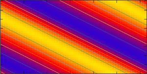
Flow fields of all types of invariant solutions, 2dRC, WVF, 3-D ribbon and tilted-vortex flow, are displayed in figure 7. The figures on the left and right in each section show the contours of  $\check w$ on the
  $xy$-plane at
  $z=0$, and on the
  $yz$-cross-section at the indicated
  $x$ stations, respectively. The streamwise independence of the 2dRC flow is of course observed in figure 7(a), while the WVF structure (figure 7b) has been discussed extensively elsewhere (see e.g. Nagata Reference Nagata1998).

Figure 7. Flow fields showing contours of  $\check {w}$ on the
  $xy$-plane at
  $z=0$ for
  $0 \leq x \leq 2{\rm \pi} /\alpha$ and
  $0 \leq y \leq 2{\rm \pi} /\beta$, and on the
  $yz$-plane at
  $x=j({{\rm \pi} }/{2\alpha }), j=0,1,2,3$ for
  $0 \leq y \leq 2{\rm \pi} /\beta$ and
  $-1 \leq z \leq 1$. (a) 2dRC at
  $\varOmega = 2.0$. (b) WVF at
  $\varOmega = 1.5$. (c) Ribbon at
  $\varOmega = 1.5$. (d) Tilted-vortex flow at
  $\varOmega = 1.75$. The colour corresponds to the numerical value of
  $\check {w}$ indicated in the colour bar on the right-hand side of each plot.
For 3-D ribbon (figure 7c) the vortex flow is characterised by a ‘double-decked’ structure. For tilted-vortex flow (figure 7d), not only  $\check w$, but all the flow quantities are found to be independent of the tilted direction.
5. Numerical integration by time
Using the converged 2dRC solution at  $\varOmega = 12.0$ as the initial value of the time-evolution code, we carry out time integration to recover the 2dRC solution at
  $\varOmega = 12.1$, in order to examine the convergence of the explicit Euler method and the explicit Runge–Kutta method of order four. The 2dRC at
  $\varOmega = 12.1$ is unstable for
  $d$ less than about 0.05 and neutral for
  $d=0$ (see figure 3a). The latter corresponds to an infinitesimal translation of 2dRC in the streamwise direction. By setting
  $\alpha =0$ in the time-evolution code, possibilities for fixed points other than 2dRC to exist are avoided. For a time step,
  ${\rm \Delta} t=0.005$, calculations blew up within 10 steps for both methods. The rate of convergence of these two methods when
  ${\rm \Delta} t=0.002$ is compared in table 5. Of course, the Runge–Kutta method converges faster than the Euler method, but because the former needs four evaluations of the right-hand side of the equation, in comparison with a single evaluation by the latter, we decided to use the Euler method with
  ${\rm \Delta} t=0.0025$ for most of the calculations.
Table 5. Convergence of the momentum transport  $M_T$ at
  $z=-1$ for 2dRC from
  $\varOmega = 12.0$ to
  $\varOmega = 12.1$ with respect to time for parameters
  $Re=100$,
  $(\alpha , \beta )=(0.0, 1.5585)$ with truncation level
  $(L, M, N)=(5, 0, 4)$ which corresponds to 972 degrees of freedom. The time step
  ${\rm \Delta} t=0.002$. Note that only three iterations by the Newton method are required to achieve convergence of the numerical system to machine precision.

In order to check the time evolution code we first attempted a numerical realisation of the transition from 2dRC to WVF. Starting from the converged 2dRC solution obtained by the Newton iterative method at  $\varOmega = 1.243$, we increased
  $\varOmega$ to 1.244 without adding extra disturbances. Many attempts were unsuccessful, converging to the 2dRC at
  $\varOmega = 1.244$. The reason for this is that the evolution process was not able to completely deviate from the initial symmetry of 2dRC solution. The situation did not change when some extra initial disturbances were added. The initial data point which was disturbed slightly from 2dRC was neither on the unstable manifold of the fixed point for 2dRC at
  $\varOmega = 1.243$, nor on the stable manifold of the fixed point for WVF at
  $\varOmega = 1.244$. We tried several attempts, but without success. Then, we changed the direction of
  $\varOmega$; considering instead the transition from WVF at
  $\varOmega = 1.244$ to 2dRC at
  $\varOmega = 1.243$. Figure 8 shows this process. Figure 8 shows the changes in
  $M_T$ and the real part of one of the amplitudes of the 3-D amplitude coefficients
  $a_{\ell m n}\ (m\neq 0)$. The plot suggests that the flow computed by the simulation code is approaching 2dRC, although the slow rate of convergence of the amplitude coefficient
  $a^R_{011}$ may be noted.

Figure 8. The numerical realisation of the transition from WVF to 2dRC. The thick curve and the thin curve plot  $M_T$ and
  $a^R_{011}$, respectively. The small circle and the cross at the initial time step indicate
  $M_T$ and
  $a^R_{011}$, respectively, of the converged WVF solution at
  $\varOmega = 1.244$. The dashed line and the dotted line drawn between time steps 200 000 and 250 000 correspond to
  $M_T$ and
  $a^R_{011}$, respectively, of the converged 2dRC solution at
  $\varOmega = 1.243$.
Figure 9(a) includes further checks. Using the converged data for WVF at  $\varOmega = 1.5$ as the initial data, we run the time evolution code by setting
  $\varOmega$ at 1.6. We judged that the code was able to numerically realise the transition from WVF at
  $\varOmega = 1.5$ to WVF at
  $\varOmega = 1.6$ after 20 000 time steps. Then,
  $\varOmega$ was increased to 1.7 and held at this value up to 50 000 time steps, and then fixed at 1.8 thereafter up to 70 000 time steps, and so on, as shown in the figure. The code seems to capture periodic solutions at
  $\varOmega = 1.8$, 1.78 and 1.76. We first supposed that the calculation converged to WVF at
  $\varOmega = 1.7$ after 50 000 time steps, but when the execution of the code was continued maintaining
  $\varOmega$ at 1.7 after 50 000 time steps, the calculation began to capture the tilted-vortex flow at around 75 000 time steps. Figure 9(b) shows the momentum transports both in the streamwise direction,
  $M_T={\mbox {d}U}/{\mbox {d}z}$ where
  $U=U_B + \check U$, and in the spanwise direction,
  ${\mbox {d}V}/{\mbox {d}z}$ where
  $V=\check V$, at
  $z=-1$.

Figure 9. (a) The numerical realisation of the transition from WVF to periodic flow. The rotation rate  $\varOmega$ is increased instantaneously from 1.7 to 1.8 at
  $\textrm {time}=50\,000$, and to
  $\varOmega =1.78$ and 1.76 instantaneously at 70 000 and 80 000 time steps, respectively. (b) The numerical realisation of transition from WVF to tilted-vortex flow.
  $\varOmega$ is kept at 1.7 all through up to 90 000 time steps. The thick curve with small plus signs and the thin curve correspond to the momentum transport
  $M_T = {\mbox {d}U}/{\mbox {d}z}$ at
  $z=-1$ in the streamwise direction and
  ${\mbox {d}V}/{\mbox {d}z}$ at
  $z=-1$ in the spanwise direction, respectively. For both top and bottom cases,
  $\varOmega$ is switched to 1.7 at time steps 20 000 after WVF at
  $\varOmega = 1.6$ has been established.
As figure 9(a) shows, the oscillation amplitude for the periodic solutions decreases when  $\varOmega$ is decreased from 1.8 to 1.76. It is of interest to search from where the periodic flow originates. Figure 10 shows that the periodic solution at
  $\varOmega = 1.75$ still maintains its periodic form, but when
  $\varOmega$ is changed to 1.74, the periodic amplitude begins to damp out and the flow appears to be approaching WVF at around 115 000 time steps, but the flow then eventually converges to the tilted-vortex flow.

Figure 10. The numerical realisation of the transition from periodic flow at  $\varOmega = 1.75$ to tilted-vortex flow at
  $\varOmega = 1.74$. The upper shorter and the lower longer dashed lines indicate the values of
  $M_T$ for tilted-vortex flow and WVF, respectively, obtained by the Newton iterative scheme.
A more detailed search for the origin of the periodic flows can be found in figure 11. Using the periodic solution at  $\varOmega = 1.75$ at 100 000 time steps in figure 10,
  $\varOmega$ is decreased to 1.747 (figure 11a) and to 1.748 (figure 11b). Although the time-evolution code converges to the tilted-vortex flow for both cases, the oscillation amplitude, before the tilted-vortex flow takes over, stays constant for
  $\varOmega = 1.748$, while it is slowly decreasing for
  $\varOmega = 1.747$. We conclude that the bifurcation of the periodic flow takes place at
  $\varOmega$ between 1.747 and 1.748, which agrees well with the Hopf bifurcation at
  $\varOmega _H = 1.7475$ described in Section 4.3. It is found that the periodic flow is a standing wave, whose waviness is inherited from WVF.

Figure 11. Numerical realisation of the transition from periodic flow to tilted-vortex flow using the data shown in figure 10 for the periodic flow at  $\varOmega = 1.75$ at 100 000 time steps as the initial condition: (a)
  $\varOmega = 1.748$; (b)
  $\varOmega = 1.747$. The two dashed lines at 25 000 time steps indicate the
  $M_T$ values for tilted-vortex flow and WVF at the corresponding
  $\varOmega$. The amplitude of the periodic flow is maintained in (a), whereas it tends to decline and approach WVF in (b). The envelopes of the periodic amplitude are drawn for reference.
6. Summary
The bifurcation structure of the early stage in RPCF is analysed numerically by using and combining both a Newton iterative scheme and a time-evolution code. The obtained  $\varOmega$ values of the bifurcation points are summarised in table 6 for
  $Re=100$ and
  $(\alpha , \beta )=(0.1, 1.5585)$.
Table 6. Bifurcation points determined at the truncation level  $(L, M, N)=(5,4,4)$ (see also figure 5b). It has been shown that the overall bifurcation structure changes only slightly when the resolution is increased (Nagata et al. Reference Nagata, Song and Wall2019), where
  $(L, M, N)=(17, 25, 7)$ is adopted for the Newton iterative method and
  $(Nx, Ny, Nz) =(28,24,24)$ is used for a direct numerical simulation (DNS) with a pseudo-spectral method for the periodic streamwise and spanwise directions and the Chebyshev tau methods for high-order finite-difference scheme in the wall-normal direction. With these numerical parameters
  $\varOmega _1 = 1.24815$ and
  $\varOmega _3 \approx 1.81$, and the DNS captured the transition from WVF at
  $\varOmega = 1.71$ to the tilted-vortex flow at
  $\varOmega = 1.72$, and detected periodic-vortex flows for
  $\varOmega \geq 1.775$. The values of the momentum transport
  $M_T$ at
  $\varOmega = 1.5$ are
  $-0.120377 \times 10^3$ for
  $(L, M, N)=(17, 25, 7)$ and
  $-0.120485 \times 10^3$ for the DNS, respectively, which can be compared with the values in table 1.

It has been taken for granted that the streamwise-independent flow, 2dRC, is the first flow to bifurcate from the basic state with increasing  $\varOmega$, and that successive bifurcations of 3-D flows follow, but the present study shows that, in fact, 2dRC is not stable from the bifurcation point at which it comes into existence, being unstable to streamwise long-wave disturbances. The tilted-vortex flow, newly found in this study, would instead be realised in place of 2dRC if streamwise wavenumbers smaller than that used here
  $(\alpha =0.1)$ were allowed to be selected. In fact, the 2dRC observed in experiments by Kawata & Alfredsson (Reference Kawata and Alfredsson2016a) is not strictly streamwise-oriented, but slightly tilted away from the streamwise direction. The tilted angle
  $\gamma =0.09$ can be measured from their figure 3 (a). This value would correspond to
  $\alpha =0.14$ for
  $\beta =1.5585$ in our analysis. If
  $\alpha$ had been set slightly larger than 0.1 in the present study, our
  $\gamma$ would have agreed better with the experimental value. Although one may think that the 2dRC has been affected by the difference in the boundary conditions in the spanwise direction, namely, the free surface at the top and the rigid end at the bottom used in the experiment, the present study clearly shows that the tilted-vortex flow exists intrinsically as an invariant solution. Furthermore, another newly found flow for RPCF in this study, periodic-vortex flow, may be involved in the complicated time-dependent behaviour observed at the onset of instability of the basic flow by Hiwatashi et al. (Reference Hiwatashi, Alfredsson, Tillmark and Nagata2007).
The time-developing code showed a temporal evolution before it eventually settled down to one of the invariant solutions or the periodic flow. No chaotic motions were detected.
It is of interest to examine the involvement of the tilted-vortex flow and the periodic-vortex flow in determining the flow structure before the WVF takes over at larger  $\varOmega$ than we investigated in this paper. It is also of interest to study bifurcations with respect to the Reynolds number, in particular, to analyse the large-scale motions, such as those in Kawata & Alfredsson (Reference Kawata and Alfredsson2016b), which is beyond the scope of the present study.
Acknowledgements
M.N. would like to thank OIST (Okinawa Institute of Science and Technology) in Japan through Professor Pinaki Chakraborty and Doshisha University in Japan through Professor Katsuya Hirata for their hospitality during his stay at their institutes. M.N. derived the theory and carried out most of the computations by iMac, B.S. performed the simulations with higher resolution on TianHe-1(A) at the National Supercomputer Center in Tianjin and D.P.W. carried out the calculations with higher truncation levels. All authors contributed equally to reaching conclusions, and in writing the paper.
Funding
This work was partially supported by the National Natural Science Foundation of China (M.N. and B.S., grant number 91752113); and the Grants-in-Aid for Scientific Research by the Japan Society for the Promotion of Science (D.P.W., grant number 18K03451).
Declaration of interest
The authors report no conflict of interest.


