


1 Introduction
In many instances leading to the fragmentation of a liquid volume, a liquid sheet, either occurring transitorily in a natural process or intentionally tailored by a dedicated device, is the last but one step before the formation of drops. The last step is the formation of ligaments, which may come from the destabilization of the sheet edge, or may arise from the coalescence of holes piercing the sheet. These holes may themselves nucleate spontaneously as a result of traces of impurities, or of defects in the liquid; they may also be the result of the amplification of an instability, or of an external action (see e.g. the review in Néel & Villermaux (Reference Néel and Villermaux2018)).
Overall, these intermediate steps, each suffering its own variability, both contribute to broadening of the final drop size distribution by favouring the emergence of very fine droplets in particular, with possible deterring consequences in some practical situations: for instance, spray drift is a major concern in agriculture. Standard flat fan atomizers (forming an expanding liquid sheet) used to spray fields with fertilizers and pesticides produce broad size distributions of droplets, a notable fraction of which have diameters below  $100~\unicode[STIX]{x03BC}\text{m}$ (hence called ‘fines’) and are likely to be swept by the wind, reaching the neighbouring farmer’s field who may not like it, or the river next to it (Hewitt Reference Hewitt2000; Kooij et al. Reference Kooij, Sijs, Denn, Villermaux and Bonn2018). Strategies to reduce their relative number are the subject of active research (Hilz et al. Reference Hilz, Vermeer, Cohen Stuart and Leermakers2012; Vernay, Ramos & Ligoure Reference Vernay, Ramos and Ligoure2015) but a detailed knowledge of the microscopic processes at play in their formation is still lacking.
One ingredient explaining the existence of fines lies in the ligament dynamics itself, which, as it breaks up, may intrinsically produce droplets of different sizes, called ‘satellites’. Capillary instabilities responsible for the ultimate breakup of an initially smooth ligament may follow each other sequentially, as was already visible in Plateau’s experiments with olive oil (Plateau Reference Plateau1873), a phenomenon which has been since then identified in related contexts involving viscous fluids (Brenner, Shi & Nagel Reference Brenner, Shi and Nagel1994; Wong et al. Reference Wong, Simmons, Decent, Parau and King2004; Villermaux, Pistre & Lhuissier Reference Villermaux, Pistre and Lhuissier2013), not to mention viscoelastic fluids where the phenomenon is the rule (Oliveira & McKinley Reference Oliveira and McKinley2005). The direct consequence of this scenario is the typically bimodal character of the drop size distribution in the spray, which presents two broad but well separated peaks (see e.g. Basaran, Gao & Bhat (Reference Basaran, Gao and Bhat2013) in the context of inkjet printing), and even a fractal sequence of iterated peaks when the cascade has the chance to persist over multiple steps (Tjahjadi, Stone & Ottino Reference Tjahjadi, Stone and Ottino1992). With water, however, the capillary breakup is so fast that the phenomenon is virtually absent, unless altered by ad hoc perturbations (Lafrance & Ritter Reference Lafrance and Ritter1977). Also, ligaments may not be smooth from the start, and it is known that pre-existing random corrugations of their cross-section induce continuous, positively skewed drop sizes repartitions (Eggers & Villermaux Reference Eggers and Villermaux2008).

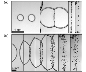
Figure 1. Two examples of the phenomenon studied here: rims of two holes expanding in a water film collide and eventually fragment into drops: (a)  $We=51$; (b)
  $We=120$. Note, in each case, the formation of a secondary sheet on the second frame, which may itself breakup into finer droplets as in (b). Frames are separated by 1 ms.
Another ingredient was discovered by Lhuissier & Villermaux (Reference Lhuissier and Villermaux2013) in the context of sheet breakup, more precisely for sheets which nucleate multiple holes, a process called ‘effervescent atomization’. Because surface tension forces are not balanced at their rim, holes grow and eventually merge with neighbouring growing holes in the sheet plane. The merging event may simply consist in an inelastic coalescence of the rims or, if the collisional rims are sufficiently fast and thick, may trigger a splash, as seen in figure 1. This is the cylindrical version of the binary impact of spherical drops problem (Bradley & Stow Reference Bradley and Stow1978; Ashgriz & Poo Reference Ashgriz and Poo1990; Roisman Reference Roisman2004). The phenomenon, also visible in the collapse of elongated sheets (Lejeune & Gilet Reference Lejeune and Gilet2019), is very similar to the one known for drops impacting a solid (see Worthington (Reference Worthington1876), Riboux & Gordillo (Reference Riboux and Gordillo2015) and the review in Josserand & Thoroddsen (Reference Josserand and Thoroddsen2016)), or a layer of the same liquid (Thoroddsen Reference Thoroddsen2002; Agbaglah & Deegan Reference Agbaglah and Deegan2014), as well as for the water entry of a solid in a pool (Worthington Reference Worthington1908; Wagner Reference Wagner1932). It produces, right upon impact, a thin fast lamella ejected from the impact point in the direction perpendicular to the collision plane, at the edge of which small (compared with the impacting rims diameter) droplets are formed; this is the way fines are produced by this process.
The existence of this mechanism has not been mentioned by the early contributors to the science of liquid sheet disintegration (Fraser et al. Reference Fraser, Eisenklam, Dombrowski and Hasson1962; Dombrowski & Johns Reference Dombrowski and Johns1963) nor in the more recent literature including the technical textbooks on atomization processes (Lefebvre Reference Lefebvre1989; Bayvel & Orzechowski Reference Bayvel and Orzechowski1993), although the spontaneous formation of holes on sheets was known (Dombrowski & Fraser Reference Dombrowski and Fraser1954), and although dispersing a minute fraction of a pressurized gas phase within the liquid to be fragmented was known to decrease considerably the mean droplet size (Sovani, Sojka & Lefebvre Reference Sovani, Sojka and Lefebvre2001).
The present work is an attempt at filling this gap, by the study of the impact dynamics of two liquid rims receding towards each other, colliding and fragmenting. The emergence of a transverse lamella at impact is first presented in § 3 and its dynamics, including its stability, is investigated in § 4. The fragmentation properties of this protocol are discussed in § 5, finally offering a comprehensive description of and explanation for the origin of the so-called fines in this context. We conclude in § 6 by suggesting possible applications.
2 Experiments
We investigate the collision of two liquid rims of individual radius  $a$, driven towards each other with relative velocity
  $2V$. The experiments presented here are performed with water at room temperature, and concern high velocity impacts of small objects: surface tension and inertia dominate the dynamics. Other effects (gravity, viscosity) are negligible, as seen from the corresponding values of the Reynolds number
  $Re\gg 1$, Ohnesorge number
  $Oh\ll 1$ and Bond number
  $Bo\ll 1$ shown in table 1. The collision is thus completely described by a single Weber number
  $We$ comparing inertia with surface tension forces
 $$\begin{eqnarray}We=\frac{\unicode[STIX]{x1D70C}(2V)^{2}2a}{\unicode[STIX]{x1D70E}},\end{eqnarray}$$
 with  $\unicode[STIX]{x1D70E}$ and
  $\unicode[STIX]{x1D70C}$ the liquid/air surface tension, and density, respectively. The collision Weber number is typically larger than unity, suggesting that a large reservoir of inertia is available to divide finely the liquid constitutive of the rims. Both rims are connected to each other by an interstitial static film with thickness
  $h$ (figure 2). Mass and momentum balances applied to the rim impose its retraction to be made at the constant Taylor (Reference Taylor1959)–Culick (Reference Culick1960) velocity
  $V=\sqrt{2\unicode[STIX]{x1D70E}/\unicode[STIX]{x1D70C}h}$ so that
  $We$ in (2.1) simply reads as the ratio of the only two geometrical parameters of the problem
 $$\begin{eqnarray}We=16\frac{a}{h}.\end{eqnarray}$$
Figure 2. Symmetric collision of liquid rims connected by a thin film (liquid portions are in darker shades). (a) Impact of toroidal rims, observed in the plane  $Oxz$ of the film. Consecutive frames are separated by 0.37 ms. (b) Idealized view of the impact of cylindrical rims, infinite in the
  $z$-direction. (c) Sketch of the emergence and destabilization of the lamella after impact (see the text, §§ 4.1–4.4).
Table 1. Typical expressions, orders of magnitude and ranges considered here of the dimensionless numbers ruling the collisions, with velocity  $V$, of an object of size
  $a$, under a gravitational field
  $g$. The liquid has a density
  $\unicode[STIX]{x1D70C}$, dynamic viscosity
  $\unicode[STIX]{x1D702}$ and its interface with air has surface tension
  $\unicode[STIX]{x1D70E}$.

2.1 Collision of toroidal rims
The impact configuration with two infinite liquid cylinders, which will be analysed in § 4, is of course an idealized view. Instead of cylinders, the experiment consists in colliding two liquid tori, which constitute the edges of two circular holes opening in the static film at the same Taylor–Culick velocity (figure 2a). The latter are nucleated simultaneously, initially separated by a distance  $b$. They thus travel for a time
  $b/2V$ from the film rupture to the rims impact. The volume of each torus
  $2\unicode[STIX]{x03C0}^{2}a^{2}b/2$ is equal to the liquid volume of the film filling the hole
  $\unicode[STIX]{x03C0}(b/2)^{2}h$, so that, at leading order, the Weber number can be written as
 $$\begin{eqnarray}We=\frac{8}{\sqrt{\unicode[STIX]{x03C0}}}\sqrt{\frac{b}{h}}.\end{eqnarray}$$
 The intensity of the collision is therefore computed from directly accessible experimental control parameters  $b$ and
  $h$, the latter being measured via the film receding velocity. The higher-order contributions from the expanding, toroidal geometry are given in § A.1.
The impact geometry exhibits at least two planes of symmetry, which are independently monitored in two experimental configurations described in the following. In the plane of the interstitial film, we denote by  $x$ the direction joining the film puncture points, and
  $z$ the orthogonal direction: invariant in the infinite cylinders problem (see figure 2b for a three-dimensional representation). All liquid reorganization during impact occurs in the direction perpendicular to that plane, referred to as
  $y$. The transverse, or mid-plane
  $Oyz$, where
  $O$ is the symmetry mid-point between the two puncture points, is the second symmetry plane in that binary symmetric configuration.
2.2 Controlled rim production
The first set-up observes the collision in the transverse plane  $Oyz$, orthogonal to the punctured interstitial film, with a slight inclination angle above the latter. By symmetry, it embraces all the dynamics following the impact, from the initial extension of a transverse lamella to the fragmentation later stages.

Figure 3. Controlled rim production set-up. The impact transverse plane  $Oyz$ is monitored, with a slight angle above the interstitial film plane. (a) Global view of the experiment: a Savart sheet (see text) surrounded by two couples of electrodes (framed detail). (b) Time lapse zoomed in downstream of the electrodes, from the simultaneous sparks to the encounter of the holes and rim impact. Consecutive frames are separated by 0.57 ms.
The film is a horizontal smooth Savart sheet, a radially expanding film resulting from the impact and deflection of a laminar circular jet with diameter  $d_{jet}$, on a slightly larger target (Savart Reference Savart1833). The velocity field in the suspended film is strictly radial, with a constant speed
  $U$, uniform across the film thickness. It is essentially equal to the jet velocity as soon as viscous dissipation on impact is negligible, which is the case with water (Villermaux et al. Reference Villermaux, Pistre and Lhuissier2013). At steady state and with water considered incompressible, the volume flux
  $2\unicode[STIX]{x03C0}Urh(r)$, with
  $h(r)$ the film thickness and
  $r$ the radial coordinate centred on the impinging jet axis, is constant throughout the jet and the sheet so that the sheet thickness decreases with the distance
  $r$ to the jet as
 $$\begin{eqnarray}h(r)=\frac{d_{jet}^{2}}{8r}.\end{eqnarray}$$
 Holes in the sheet are punctured by two simultaneous electrical sparks transpiercing the sheet by vaporizing the liquid locally. They are triggered on demand, by means of two couples of electrodes connected to large capacitors which on discharge produce the two simultaneous sparks. The electrodes are located on both sides of the film, separated by approximately a millimetre (the film is thinner than  $100~\unicode[STIX]{x03BC}\text{m}$ there), at the same radial location
  $r_{0}$ from the jet, and separated by an azimuthal angle
 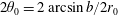 $2\unicode[STIX]{x1D703}_{0}=2\arcsin b/2r_{0}$ (
 $b$ is the Euclidean distance between the puncture points, figure 3a). As the holes grow and feed the rims, they are advected outwards, on diverging radial trajectories (figure 3b). This way, rims travel a distance larger than
  $b/2$ before they collide (see § 2.1), and hence have collected a priori more liquid when they come into contact. On the other hand, due to the thickness decrease (2.4), they experience an increasing opening velocity
  $V$, which now depends on the current radial coordinate:
  $V(r)=\sqrt{16r\unicode[STIX]{x1D70E}/\unicode[STIX]{x1D70C}d_{jet}^{2}}$. The impact Weber number is eventually increased, when compared with the static and uniform film case. However, for small angles
  $2\unicode[STIX]{x1D703}_{0}\sim b/r_{0}$, it simplifies back to the static film case (2.3). The exact expression is derived in § A.2, along with the experimental deviations to the static film approximation. Although the exact expression in (A 11) is preferred when presenting the experimental results below, we use the approximate expression (2.3) when comparing this set-up and the second one described in § 2.3.
The advected impact is observed in the laboratory fixed frame, with a high-speed camera and backlighting. Within the range of Weber numbers investigated (from 40 to 200), the set-up is time and space resolved, thanks to frame rates up to 50 kHz and spatial resolutions around  $30~\unicode[STIX]{x03BC}\text{m}$ per pixel.
2.3 Random rim production
The second set-up allows us to observe the rims’ collision and subsequent fragmentation in the plane  $Oxz$, the liquid film being a Savart sheet as before. Now, film punctures are nucleated by internal defects, bubbles incorporated into the liquid prior to the formation of the film (see Lhuissier & Villermaux (Reference Lhuissier and Villermaux2013) for a complete description of the set-up and method). Bubbles embedded in the sheet pop up at some distance along their radial trajectory, making the film rupture location a random variable. As a result, the location of the subsequent impact of neighbouring rims, following the merging of two growing holes, is also a distributed random variable (a single collision is illustrated in figure 4).

Figure 4. Random rim production set-up. Time lapse of a selected impact event, observed in the interstitial film plane. (a) Holes opening and rim growth, impact, destabilization and late fragmentation. Consecutive frames are separated by 1 ms. Grey dashed lines are the radial trajectories of the rims centre, advected at the constant speed  $U$. (b) Fragment detection and area-based size measurement.
The monitored field of view is large ( $4\times 4~\text{cm}^{2}$, with a resolution of
  $40~\unicode[STIX]{x03BC}\text{m}$ per pixel) and focuses on a restricted angular sector of the Savart sheet, around the radius where most of the punctures take place. Together with a low acquisition frame rate (1 kHz), it allows recording of a large number of impact events. The careful selection and a posteriori characterization of some 560 hole openings constitutes a batch of 280 rim impacts. The frame rate is high enough to enable the individual tracking of the rims, from the moment they appear to the collision and, later, their destabilization into drops (figure 4). However, most of hole openings and rim impacts occur between two recorded frames. The respective time instants of the punctures and of the collision are determined with a greater precision by a linear interpolation between those two frames, on the basis of the following approximations. The film thickness is considered uniform along each rim trajectory, so that the latter are assumed to open circularly, at the constant Taylor–Culick velocity. Meanwhile, they are advected outwards with the constant radial flow of the Savart sheet, so that there is, for each couple of rims, a unique impact point. The computation of the Weber from (2.3) is made under these approximations. As explained in § 2.1, it underestimates the actual value of
  $We$, for which there is here no straightforward expression, but enables the comparison with the first set-up when needed (§ 2.2). For two slightly asynchronous hole punctures, resulting in an asymmetric impact, the Weber number is based on the radius
  $a$ of the smallest rim.
2.4 Fragments
Drops are individually detected, and calibrated. Sizes correspond to drops which have relaxed to a spherical shape and are in focus only, in both set-ups (figures 4b and 5). Their diameter  $d$ is based on the measurement of their projected area
  $\unicode[STIX]{x03C0}d^{2}/4$, the quality of the pictures allowing for a basic intensity thresholding. Discrepancies between both set-ups are described in appendix B. Furthermore, the time-resolved monitoring of the transverse plane in the controlled rim production set-up (§ 2.2) provides extensive data about the ejection velocity of the fragments (figure 5).

Figure 5. Snapshot of the transverse plane after a collision at  $We=193$, along with droplet size and velocity detection. The uniform advection velocity
  $U$ is substracted during the data processing. The solid line is the axial centre line of the merged rim, the dashed lines its initial upper and lower extents prior to the collision.
3 Phenomenology
With the combination of the two set-ups depicted in the previous section, the Weber number of the impact is varied from 10 to 200. In this range, for a single and well-identified impact event, a variety of behaviours are observed. We describe the three successive steps leading to the formation of fines, whose analysis will be made in §§ 4 and 5.
3.1 Unstable transverse lamella
The collision of two rims is inelastic. Even for an impact at low  $We$ leading ultimately to a unique cylinder with section
  $2\unicode[STIX]{x03C0}a^{2}$ (mass conservation), most of the incident kinetic energy is lost in internal irregular motions. We will come back to this point in § 5.1. However, since
  $Oh$ is low in the present case, the dissipation scale (
 ${\sim}h\times Oh$, see Culick (Reference Culick1960)) is much smaller than
  $a$, and the collision gives rise to an – essentially inviscid – dynamics involving large deformations of the merging rims. Notably, the emergence of a thin lamella, in the direction orthogonal to the impact direction (figure 6) is systematically observed for
  $We$ greater than 50. This expanding lamella is itself bordered by a rim at its extremity in
  $y=\ell (t)$, which is uniform along the rims’ axis in the
  $z$-direction. This secondary rim is pulled back by surface tension conferring to
  $\ell (t)$ an ever decelerated motion. The phenomenon is particularly clear from the angle of view offered by the controlled rim production set-up (see also figure 10).

Figure 6. Lamella emergence and growth, in the transverse plane, for a  $We=83$ collision. Consecutive frames are separated by
  $22~\unicode[STIX]{x03BC}\text{s}$ (from top to bottom, then left to right).

Figure 7. Longitudinal destabilization of a transverse growing lamella, for a  $We=102$ collision. Consecutive frames are separated by
  $80~\unicode[STIX]{x03BC}\text{s}$.
The larger  $We$, the larger the lamella maximal extension. As a consequence, the overall extension–retraction time of the lamella, i.e. its oscillation period or lifetime, increases when
  $We$ is increased, as will be shown in § 4.1. Regularly spaced indentations of the lamella rim (figure 7) are markedly apparent as
  $We$ is increased. This longitudinal destabilization (
 $z$-direction) features a wavelength
  $\unicode[STIX]{x1D706}$. It is a signature of the deceleration undergone by the lamella in the course of its development as will be analysed in § 4.4.
3.2 Transverse ligaments and the production of fines
Above a critical Weber number of the order of  $We_{c}\approx 66$, the longitudinal indentations of the lamella rim give rise to regularly spaced, transverse ligaments (figures 8 and 14). The breakup of these secondary ligaments eventually forms small droplets, the fines, which are expelled, in continuation of the lamella transverse growth, in the direction perpendicular to the main liquid sheet (figure 8). These objects substantially alter the overall drop size distribution of the resulting spray, as will be seen in § 5.2.
Through this process of lamella expansion, indentation growth, ligament formations and breakup, increasingly many, and smaller, droplets (relative to  $a$) are formed as
  $We$ is increased. They are, since the colliding rims are more finely divided, not only obviously all the more numerous (figure 9d–f) but are also more distributed in size relative to their mean, as will be seen in § 5.2.

Figure 8. Formation of secondary transverse ligaments, and ejection of fine, fast droplets from their tips, for a  $We=193$ collision. Consecutive frames are separated by
  $38~\unicode[STIX]{x03BC}\text{s}$.
4 Collision
The impact of identical rims is considered in the infinite cylinder limit (figure 2b). Apart from the two planes of symmetry already identified – the plane of the interstitial film and the transverse mid-plane between the rims, see § 2.1 – the situation is invariant along the rims’ axis and consequently all reasonings involving mass, force, energy, etc. are made per unit length in this direction.

Figure 9. Snapshots of the rims before (a–c) and after (d–f) impact, at time  $t=40\,a/V$, for three increasing
  $We=62$ (a,d), 113 (b,e) and 193 (c,f). All pictures are scaled on the colliding rim radius
  $a$, with dimensions
  $30\times 15$ (a,b,c,g) and
  $60\times 30$ (d–f). Scale bar width is 1 mm. (g) Rim corrugations before impact, as a function of
  $We$. The solid line is the best linear fit (see (5.3)).
4.1 Global collision dynamics, the long time and length scales
Let two parallel cylinders aligned along  $z$ and travelling at relative speed
  $2V$ along
  $x$ collide, thus adding up their mass and deflecting the momentum they carry along the transverse
  $y$-axis (equally split in both positive and negative directions). The fused cylinders expand along
  $y$ until the unbalanced surface tension force at the surface of the ensemble limits its growth. The phenomenon is reminiscent of the oscillatory dynamics of jets issuing from a non-circular orifice undergoing peristaltic pulsations studied by Rayleigh (Reference Rayleigh1879) and others (see § 6 in Eggers & Villermaux (Reference Eggers and Villermaux2008) for a historical perspective).
In all inertial fluid mechanics problems, the displacement of the fluid particles reflects the structure of the pressure field. The pressure might be viewed as the source of the motion (Cooker & Peregrine Reference Cooker and Peregrine1995; Antkowiak et al. Reference Antkowiak, Bremond, Dizès and Villermaux2007), or a consequence of it (Birkhoff et al. Reference Birkhoff, MacDougall, Pugh and Taylor1948; Riboux & Gordillo Reference Riboux and Gordillo2014), but in each case both are linked.
Ignoring first the fine details of the collision at short times, it is easy to anticipate the time scale (oscillation period  $T$), and length scale (maximal extension of the ensemble
  $L$) of the collision coarse-grained motion after the fusion of the cylinders (figures 6 and 10a). We sketch the deforming fused ensemble as a lamella expanding in the
  $y$-direction with length
  $\ell (t)$ and width
  $w$ so that
  $2\unicode[STIX]{x03C0}a^{2}=\ell \times w$. The liquid velocity in the
  $y$-direction is
  $v(y,t)=y\dot{\ell }/\ell$. Integration of the Euler equation
 $$\begin{eqnarray}\unicode[STIX]{x1D70C}(\unicode[STIX]{x2202}_{t}v+v\unicode[STIX]{x2202}_{y}v)=-\unicode[STIX]{x2202}_{y}p\end{eqnarray}$$
 between  $y=0$ and
  $y=\ell (t)$ with
  $p$ the liquid pressure (see Villermaux & Bossa (Reference Villermaux and Bossa2009) for the axisymmetric version of the problem) provides
 $$\begin{eqnarray}{\textstyle \frac{1}{2}}\unicode[STIX]{x1D70C}\ell \ddot{\ell }=p(0)-p(\ell ).\end{eqnarray}$$
 The pressure at the expanding extremity is  $p(\ell )\approx \unicode[STIX]{x1D70E}/w$ while the pressure at the contracting location is, in this coarse-grained description,

The Dirac delta contribution  stands for the pressure impulse caused by the impact of the cylinders at the collision location
  $y=0$ and time
  $t=0$. The momentum transfer giving rise to this pressure surge lasts in fact for the crushing time
  $a/V$, which is safely taken as zero provided the resulting motion of the fused ensemble lasts for a time much larger than
  $a/V$, as will be checked a posteriori. With
  $\ell (0)=a$, equation (4.2) amounts to


The initial velocity of the lamella is  $V$ (see also (4.12)). The period
  $T$ (obtained for
  $\ell (T)=a$) and maximal extension
  $L\equiv \ell (T/2)$ of the motion are
 $$\begin{eqnarray}\displaystyle & \displaystyle T\sim \frac{a}{V}We, & \displaystyle\end{eqnarray}$$
 $$\begin{eqnarray}\displaystyle & \displaystyle \frac{L-a}{a}\sim We. & \displaystyle\end{eqnarray}$$
 The relative maximal extension of the expanded fused cylinders  $(L-a)/a$ is a measure of the ratio of the motion period
  $T$ to the crushing time
  $a/V$. It is equal to
  $We$, a quantity larger than unity, justifying a posteriori our impulse treatment of the pressure surge. Figures 10(b) and 10(c) demonstrate the validity of the above scaling relations, up to numerical factors. The expanding lamella fragments for large
  $We$, that we describe next, explaining why the measurement of
  $T$ is meaningless above
  $We\approx 100$.

Figure 10. Lamella dynamics. (a) Space–time diagram of a slice in the transverse $y$-direction. The lamella extension
  $\ell (t)$ is underlined with (
 $+$) markers and (4.5) is shown as a solid line. (b) Lamella global expansion period
  $T$ and (c) maximal extension
  $L$ as a function of the collision parameters in (4.6) and (4.7). Solid lines are best linear fit with numerical factors: (a) 0.17 and (b) 0.027.
4.1.1 A note on scalings
In the present one-dimensional collision process, both  $L/a$ and
  $VT/a$ are proportional to
  $We$, while the same quantities are proportional to
  $\sqrt{We}$ for the impact of a drop expanding radially in two dimensions. Although mechanical energy is definitely not conserved in these problems, equating the initial kinetic energy to the surface energy of the deformed lamellae at maximal extension picks up nevertheless the correct scaling (because the amount of dissipated energy is the fraction of the initial energy, see Villermaux & Bossa (Reference Villermaux and Bossa2011), Gelderblom et al. (Reference Gelderblom, Lhuissier, Klein, Bouwhuis, Lohse, Villermaux and Snoeijer2016) and Planchette et al. (Reference Planchette, Hinterbichler, Liu, Bothe and Brenn2017) for more refined descriptions of equivalent problems, and comments on the energy conservation approach). For a drop, we have
  $\unicode[STIX]{x1D70C}a^{3}V^{2}\sim \unicode[STIX]{x1D70E}L^{2}$ which is indeed compatible with the
  $\sqrt{We}$ scaling, while here we have
  $\unicode[STIX]{x1D70C}a^{2}V^{2}\sim \unicode[STIX]{x1D70E}L$, leading to (4.7). Finally, let us also note that these scalings describe large deformations of the impacting objects (
 $L/a\gg 1$). Small oscillations about the reference state like
  $\ell \sim a(1+\unicode[STIX]{x1D716})$ and
  $w\sim a/(1+\unicode[STIX]{x1D716})$ with
  $\unicode[STIX]{x1D716}\ll 1$ lead to
  with
with  $\unicode[STIX]{x1D714}=\sqrt{4\unicode[STIX]{x1D70E}/\unicode[STIX]{x1D70C}a^{3}}$ so that
  $VT/a\sim L/a\sim \sqrt{We}$ in that limit.
4.2 Early time lamella formation
We have explained in § 3.1 that because viscous dissipation is made at a very small scale in the rims when  $Oh\ll 1$, the momentum transfer at collision leads to the formation of tiny objects, which may be formed before the rim fusion is completed (i.e. for
  $t<a/V$), hence the early emergence of a thin transverse lamella. We analyse this fine-grained aspect of the phenomenon here, exploring what happens ‘inside’ the Dirac Delta of the previous section. Two regimes are distinguished.
We describe the sudden collision at velocity  $2V$ of two liquid cylinders of radius
  $a$. The cylinders are first considered independent, moving in a dynamically inert ambient medium, contacting along their generatrix (the same reasoning holds for two spheres impacting at a point); their geometrical interpenetration radius is initially
  $r\sim \sqrt{Vat}$ (figure 2c). The induced flow
  $\boldsymbol{v}(\boldsymbol{x},t)$ ruled by
  $\unicode[STIX]{x2202}_{t}\boldsymbol{v}+\boldsymbol{v}\boldsymbol{\cdot }\unicode[STIX]{x1D735}\boldsymbol{v}=-\unicode[STIX]{x1D735}p/\unicode[STIX]{x1D70C}$ and
  $\unicode[STIX]{x1D735}\boldsymbol{\cdot }\boldsymbol{v}=0$ obeys initially, when the velocity amplitude
  $|\boldsymbol{v}|$ is small enough to neglect the convective term
  $\boldsymbol{v}\boldsymbol{\cdot }\unicode[STIX]{x1D735}\boldsymbol{v}$ (see Lamb (Reference Lamb1932), Art. 11 and Cooker & Peregrine (Reference Cooker and Peregrine1995))
 $$\begin{eqnarray}\displaystyle & \displaystyle \unicode[STIX]{x2202}_{t}\boldsymbol{v}=-\frac{1}{\unicode[STIX]{x1D70C}}\unicode[STIX]{x1D735}p, & \displaystyle\end{eqnarray}$$
 $$\begin{eqnarray}\displaystyle & \displaystyle \text{and thus }\unicode[STIX]{x1D6FB}^{2}p=0. & \displaystyle\end{eqnarray}$$
 In other words, if the liquid has moved over a distance  $r$ in the
  $y$-direction, then it has moved over the same distance in the
  $x$-direction. The consequence of the Laplacian character of the pressure is that, since
  $r$ is the only initial length scale of the problem (besides
  $a\gg r$), the net volume of liquid whose motion is slowed down (per unit cylinder length) is of order
  $r^{2}$, setting its mass
  $m\sim \unicode[STIX]{x1D70C}\,r^{2}$ (not to be confused with the deflected volume
  $Vt\,r$, feeding the ejected lamellae). The cancellation of the corresponding momentum initially carried in the
  $x$-direction gives rise to a force
  $f=V{\dot{m}}$, and therefore to an isotropic pressure at the impact point given by
 $$\begin{eqnarray}\displaystyle p(0) & {\sim} & \displaystyle \frac{f}{r}\end{eqnarray}$$
 $$\begin{eqnarray}\displaystyle & {\sim} & \displaystyle \unicode[STIX]{x1D70C}V^{2}\sqrt{\frac{a}{Vt}},\end{eqnarray}$$
an early time divergence familiar in impact problems (Wagner Reference Wagner1932; Cointe & Armand Reference Cointe and Armand1987; Philippi, Lagrée & Antkowiak Reference Philippi, Lagrée and Antkowiak2016), holding both in one and two dimensions (for the impact of a spherical drop on a solid, for instance).
The pressure gradient  $\unicode[STIX]{x2202}_{y}p$ in the symmetry plane of the impact (figure 2c) is of order
  $p(0)/r$ so that, from the dynamics in (4.8),
  $v/t\sim V/t$, giving simply
 $$\begin{eqnarray}v\sim V.\end{eqnarray}$$
 The mass in motion  $m$ increases proportionally to time as the driving force
  $p(0)\times r$ is constant, so that the velocity is constant. With this estimate for
  $v$, the amplitude of the discarded nonlinear term
  $|\boldsymbol{v}\boldsymbol{\cdot }\unicode[STIX]{x1D735}\boldsymbol{v}|$ in the Euler equation above is of order
  $V^{2}/r\sim 1/\sqrt{t}$, indeed smaller than
  $1/t$ as
  $t\rightarrow 0$. The intensity of this induced flow is smaller than the geometrical expansion velocity of the interpenetration region
  ${\dot{r}}\sim \sqrt{Va/t}$ as long as
  $t<a/V$, consistent with the empirical observation that a lamella is seen to emerge from the impact region when the interpenetration distance is a fraction of
  $a$, and that the ejection velocity of the resulting lamella (and detached droplets), is of order
  $V$ when complications with liquid viscosity, ambient medium and substrate roughness are negligible (see Xu, Barcos & Nagel (Reference Xu, Barcos and Nagel2007), Riboux & Gordillo (Reference Riboux and Gordillo2015) for drops impacts).
4.3 Very early dynamics: the tiniest ejecta
The linear pressure impulse dynamics in (4.8) does not, however, apply everywhere in the interpenetration region. Close to the contact line between the cylinders (the same remark applies to a drop impacting a solid), the velocity  $v$ in the symmetry plane of the impact is itself of order
  ${\dot{r}}$, making the nonlinear term
  $|\boldsymbol{v}\boldsymbol{\cdot }\unicode[STIX]{x1D735}\boldsymbol{v}|$ of order
  $v^{2}/\unicode[STIX]{x1D6FF}(t)$ where
  $\unicode[STIX]{x1D6FF}(t)$ is a length scale setting the width of the pressure and velocity gradients close to the contact line. If
  $\unicode[STIX]{x1D6FF}(t)$ is itself initially zero and an increasing function of time, the nonlinear term is more singular than
  $V/t$, suggesting that the early time dynamics balances inertia with pressure, at least in a small region of size
  $\unicode[STIX]{x1D6FF}$. Writing
  $p\sim f/\unicode[STIX]{x1D6FF}$ so that
  $\unicode[STIX]{x2202}_{y}p\sim f/\unicode[STIX]{x1D6FF}^{2}$, the balance between
  $|\boldsymbol{v}\boldsymbol{\cdot }\unicode[STIX]{x1D735}\boldsymbol{v}|$ and
  $|\unicode[STIX]{x1D735}p|/\unicode[STIX]{x1D70C}$ at the contact line can be written
 $$\begin{eqnarray}\frac{v^{2}}{\unicode[STIX]{x1D6FF}}\sim \frac{1}{\unicode[STIX]{x1D70C}}\frac{f}{\unicode[STIX]{x1D6FF}^{2}},\quad \text{or}\quad v\sim V\sqrt{\frac{a}{\unicode[STIX]{x1D6FF}}},\end{eqnarray}$$
 $$\begin{eqnarray}\text{providing }\unicode[STIX]{x1D6FF}\sim Vt,\quad (\text{since }v\sim {\dot{r}})\end{eqnarray}$$
 so that the local pressure in the contact line region (Mandre, Mani & Brenner Reference Mandre, Mani and Brenner2009) is now of order  $f/\unicode[STIX]{x1D6FF}\sim \unicode[STIX]{x1D70C}Va/t$, indeed more singular than
  $p(0)$ in (4.11). Detailed calculations (Birkhoff et al. Reference Birkhoff, MacDougall, Pugh and Taylor1948; Riboux & Gordillo Reference Riboux and Gordillo2014) show that the contact line velocity is closer to
  $v=2{\dot{r}}$ (see also Philippi et al. (Reference Philippi, Lagrée and Antkowiak2016) for a fully self-similar description), albeit affected by viscous corrections when a no-slip condition applies. Expressing that the deflected mass
  $\unicode[STIX]{x1D70C}Vt\,r$ all enters the ejected lamella which carries its momentum provides the lamella thickness
  $w$ as
  $V\unicode[STIX]{x2202}_{t}(\unicode[STIX]{x1D70C}Vtr)\sim \unicode[STIX]{x1D70C}v^{2}w$, that is
  $w\sim (V/a)r^{2}/{\dot{r}}\sim t^{3/2}$ (and consistently
  $w<\unicode[STIX]{x1D6FF}$ as
  $t\rightarrow 0$).
Note on dimensionality: the reasoning above also applies to a drop of radius  $a$ impacting a solid or another identical drop, expanding in two dimensions with now
  $m\sim \unicode[STIX]{x1D70C}r^{3}$ leading, from
  $f\sim V{\dot{m}}$, to
  $v\sim V(a/\unicode[STIX]{x1D6FF})$ and
  $p\sim f/(r\unicode[STIX]{x1D6FF})\sim \unicode[STIX]{x1D70C}V^{2}(a/\unicode[STIX]{x1D6FF})$, identically to the one-dimensional case (see e.g. Riboux & Gordillo Reference Riboux and Gordillo2014).
We now consider the case of cylinders initially linked by a quiescent film of thickness  $h<a$ relevant to the present situation (the thickness
  $h$ is in practice related to the velocity
  $V=\sqrt{2\unicode[STIX]{x1D70E}/\unicode[STIX]{x1D70C}h}$ by the Taylor–Culick relation). The presence of the film de-singularizes the pressure at contact since it is both uniform and finite over a region of order
  $h$. The above reasoning thus starts to apply as soon as
  $\unicode[STIX]{x1D6FF}=h$, suggesting, given
  $v\sim V\sqrt{a/\unicode[STIX]{x1D6FF}}$ in (4.13), that the ejection speed of the lamella at very short times, possibly fragmented into very fine droplets above a critical Weber number
  $We_{c}$ to be determined (next § 4.4), will be of order
 $$\begin{eqnarray}\displaystyle V_{e} & {\sim} & \displaystyle V\sqrt{\frac{a}{h}}\end{eqnarray}$$
 $$\begin{eqnarray}\displaystyle & \propto & \displaystyle V\sqrt{We-We_{c}},\end{eqnarray}$$
a dependence to which the observations reported in § 5.4 below give some support.
This very early dynamics holds as long as  $\unicode[STIX]{x1D6FF}<r$, that is
  $t<a/V$, then leaving place to the one in § 4.2.

Figure 11. Longitudinal instability. (a) Growth time  $\unicode[STIX]{x1D70F}$ and (b) wavelength
  $\unicode[STIX]{x1D706}$ are plotted against their expected scalings
  $h/V$ and
  $h$, respectively from (4.19), collapsing data from impacts at different
  $We$. Solid lines are best linear fits with factors: (a) 47 and (b) 3.9.
4.4 Lamella deceleration and instability
Once ejected from the interpenetration region with a thickness of order  $h$, the lamella expands ballistically, only arrested at its border by capillary retraction, thus giving rise to an ever decelerated regime. The corresponding dynamics for
  $\ell (t)$ then simply reads
 $$\begin{eqnarray}\ddot{\ell }\sim -\frac{\unicode[STIX]{x1D70E}}{\unicode[STIX]{x1D70C}h^{2}},\end{eqnarray}$$
 featuring a negative and constant acceleration. The lamella border is a density interface which separates a dense liquid from a dynamically inert medium. Being decelerated, this interface is unstable in the sense of Rayleigh–Taylor, a fact which is commonplace for slowing (Villermaux & Bossa Reference Villermaux and Bossa2011), retracting (Lhuissier & Villermaux Reference Lhuissier and Villermaux2011) or spinning sheets (Fraser, Dombrowski & Routley Reference Fraser, Dombrowski and Routley1963; Eisenklam Reference Eisenklam1964), explaining the origin of the developing longitudinal indentations observed in the  $z$-direction (figure 7). The characteristic time of growth
  $\unicode[STIX]{x1D70F}$, and wavelength
  $\unicode[STIX]{x1D706}$ of this instability are
 $$\begin{eqnarray}\unicode[STIX]{x1D70F}\sim \sqrt{\frac{\unicode[STIX]{x1D706}}{|\ddot{\ell }|}};\quad \unicode[STIX]{x1D706}\sim \sqrt{\frac{\unicode[STIX]{x1D70E}}{\unicode[STIX]{x1D70C}|\ddot{\ell }|}},\end{eqnarray}$$
 which translate, given  $\ddot{\ell }$ in (4.17), to
 $$\begin{eqnarray}\unicode[STIX]{x1D70F}\sim \frac{h}{V};\quad \unicode[STIX]{x1D706}\sim h.\end{eqnarray}$$
 These relationships are relatively convincing at the scaling level (they offer a good collapse for different  $We$, in particular), with however large pre-factors, as seen from figure 11.

Figure 12. Onset of the instability. Lamella oscillation period  $T$ (hollow circles) and instability growth rate
  $\unicode[STIX]{x1D70F}$ (plain triangles), in units of the crushing time scale
  $a/V$ versus
  $We$. Dashed and solid lines are the predicted scalings from (4.20), along with best fit amplitudes. They cross at the instability threshold and define
  $We_{c}\simeq 66$.
4.5 Transition to splashing
The global oscillation period of the fused cylinders  $T$ given in (4.6), and the lamella instability time scale
  $\unicode[STIX]{x1D70F}$ in (4.19) both written in units of
  $a/V$ depend on the Weber number as
 $$\begin{eqnarray}T\sim \frac{a}{V}We;\quad \unicode[STIX]{x1D70F}\sim \frac{a}{V}We^{-1}.\end{eqnarray}$$
 One is longer (namely  $T$) and the other shorter (namely
  $\unicode[STIX]{x1D70F}$) when
  $We$ increases. Obviously, a cross-over occurs whose meaning is the following: at moderate
  $We$, the expansion–recoil period of the fused rims is too short for the expanded lamella to destabilize given its slow pace; destabilization is faster and has also more time to develop at larger
  $We$, and is thus now favoured. Both trends are visible in figure 12. The instability growth time cannot, de facto be measured below the cross-over threshold at the intersection of the two curves, which occurs for
  $We_{c}\approx 66$, a value which was qualitatively anticipated by Lhuissier & Villermaux (Reference Lhuissier and Villermaux2013).
The onset of this instability (explaining the formation of the ‘arms’ of Worthington (Reference Worthington1876)), whose outcome is the production the fines analysed in the next section, is very similar to the so-called ‘splashing’ transition in drop impact (i.e. the production of disjointed fragments besides the recoil of the main drop, see Josserand & Thoroddsen (Reference Josserand and Thoroddsen2016)) for which we have given here a mechanistic interpretation.
5 Fragmentation: the fines and their distribution
The ultimate fragments are produced from the capillary destabilization of the merged rims which are, above the splashing transition, indented into transverse ligaments. There are thus two potential sources of variability in the drop sizes, one associated with the unevenness of the fused rim cylinder due to the inelasticity of the collision, the other with the noisy capillary breakup of the secondary ligaments. We document both variabilities below over a broad range of Weber number, in order to describe the overall drop size distribution for any  $We$ in this range.

Figure 13. Corrugated rim fragmentation at low  $We$. (a) Drop sizes distribution for a
  $We=58$ impact, normalized by
  $d_{PR}=1.89\times 2\sqrt{2}\,a$. The solid line is a gamma distribution obtained from (5.1) with
  $m=5$, or with (5.8) for
  $n\rightarrow \infty$ and
  $m=5$. (b) Mean drop size
  $\langle d\rangle /h$ for increasing Weber number
  $We/16=a/h$, for both experimental set-ups. The solid line is the Plateau–Rayleigh prediction
  $\langle d\rangle /a=1.89\times 2\sqrt{2}\,We/16$ holding below
  $We_{c}$ while
  $\langle d\rangle$ tends to saturate at a value proportional to
  $h$.
$h$.
5.1 Capillary breakup with corrugations ( $We<We_{c}$)

For collisions with  $We$ below the critical splashing Weber number
  $We_{c}$, drops simply form the breakup of the fused rim cylinder, whose mean radius is
  $\sqrt{2}a$ (see e.g. figure 1a). In that case, we know that the outcome is a droplet distribution of sizes
  $d$ given by
 $$\begin{eqnarray}p(\unicode[STIX]{x1D701})=\frac{m^{m}}{\unicode[STIX]{x1D6E4}(m)}\unicode[STIX]{x1D701}^{m-1}\text{e}^{-m\unicode[STIX]{x1D701}},\quad \text{with }\unicode[STIX]{x1D701}=d/\langle d\rangle\end{eqnarray}$$
 in units scaled by their mean  $\langle d\rangle$, a mean approximately given by the standard Plateau–Rayleigh expectation
 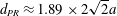 $d_{PR}\approx 1.89\times 2\sqrt{2}a$ (see figure 13a,b) modulo a weak correction on
  $m$, whose value reflects the initial relative corrugations of the cylinder (Eggers & Villermaux Reference Eggers and Villermaux2008). If, right after the collision, the cylinder radius is
  $\sqrt{2}a+\unicode[STIX]{x1D709}(z)$, with
  $\unicode[STIX]{x1D709}(z)$ a longitudinal modulation with zero mean and variance
  $\langle \unicode[STIX]{x1D709}^{2}\rangle$, then
 $$\begin{eqnarray}m\sim \frac{a^{2}}{\langle \unicode[STIX]{x1D709}^{2}\rangle }.\end{eqnarray}$$
 As seen in figure 9(a–c), the corrugations are mostly reminiscent of the state of the rims prior to the collision, and the variance  $\langle \unicode[STIX]{x1D709}^{2}\rangle$ may be interpreted from an energy balance (see the Appendix in Bremond, Clanet & Villermaux (Reference Bremond, Clanet and Villermaux2007)). Only half of the kinetic energy is used for the rim recess, the other half, ultimately dissipated by viscosity, being at the origin of turbulent-like motions, the cause of the rim interface corrugations (see the Appendix in Villermaux & Bossa (Reference Villermaux and Bossa2011)). Balancing the available kinetic energy with the (transient) surface energy excess in the corrugated state
 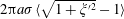 $2\unicode[STIX]{x03C0}a\unicode[STIX]{x1D70E}\langle \sqrt{1+\unicode[STIX]{x1D709}^{\prime 2}}-1\rangle$ where
  $\unicode[STIX]{x1D709}^{\prime }=\text{d}\unicode[STIX]{x1D709}/\text{d}z$, we have, at lowest order and up to (large) prefactors,
 $$\begin{eqnarray}a\unicode[STIX]{x1D70E}\langle \unicode[STIX]{x1D709}^{\prime 2}\rangle \sim a^{2}\unicode[STIX]{x1D70C}V^{2},\qquad \text{or}\quad \langle \unicode[STIX]{x1D709}^{\prime 2}\rangle \sim We.\end{eqnarray}$$
 Corrugations are injected at the scale of the incoming rims radius  $a$ which sets the fluctuation scale of
  $\unicode[STIX]{x1D709}$ so that
  $\langle \unicode[STIX]{x1D709}^{\prime 2}\rangle \approx \langle \unicode[STIX]{x1D709}^{2}\rangle /a^{2}$ (see figure 9) and
 $$\begin{eqnarray}m\sim We^{-1},\end{eqnarray}$$
 indicating that more violent collisions lead to broader size distributions [remember that ], such as that shown in figure 13(a) at
  $We=58$ for which
  $m=5$.

Figure 14. Transverse ligament mediated fragmentation, at  $We=193$. The sequence shows the emergence and destabilization of the lamella (left panel, from top to bottom), then its retraction into transverse ligaments with volume
  $s^{3}$ (central picture) which finally fragment into droplets with individual size
  $d$ (right picture).
5.2 Above the splashing transition ($We>We_{c}$)

Above the splashing transition described in § 4.5, the transverse indentations produce ligaments which fragment into increasingly many smaller drops as  $We$ is increased. Consequently, the mean drop size deviates from the Plateau–Rayleigh prediction (figure 13b) because the drops now come from the fused rim cylinder chopped off into smaller pieces, namely the finer transverse ligaments (figure 14). An estimation of the mean size of these fine droplets is as follows: assume the fused rims convert entirely (this is all the more true when
  $We$ is larger) into an assembly of transverse ligaments each with length
  $L\sim a\,We$ and spaced by
  $\unicode[STIX]{x1D706}\sim h$ (see § 4). Volume conservation gives
  $\unicode[STIX]{x03C0}(\sqrt{2}a)^{2}\unicode[STIX]{x1D706}\sim \unicode[STIX]{x03C0}L\langle d\rangle ^{2}$ with
  $\langle d\rangle$ the transverse ligament mean diameter, also setting that of the fines after capillary breakup (Plateau Reference Plateau1873; Rayleigh Reference Rayleigh1879). We thus expect, when the conversion is complete, that
  $\langle d\rangle$ will saturate at a value of order
 $$\begin{eqnarray}\langle d\rangle \sim h\end{eqnarray}$$
 above  $We_{c}$, a very different trend than the one prevailing below (for which
  $\langle d\rangle /h\sim We$, see figure 13b). Note that it is precisely because the set-up with random hole production misses the finest drops (see appendix B) that this transition is delayed compared with that observed with the controlled set-up, and which indeed occurs at
  $We_{c}$.

Figure 15. Size distribution, at  $We=193$. (a) Ligament size
  $s$ distribution, measured before (●) and after (
 $\star$) fragmentation (respectively expressions (5.6) and (5.7)), along with a gamma distribution (5.1) with order
  $m=40$ (solid line). (b) Drop size
  $d$ distribution, resulting from the transverse ligament fragmentation: (●) 322 drops, for which origin ligaments are unspecified; (
 $\star$) 117 drops issued from the ligaments in (a). The solid line is the distribution (5.8) with orders
  $m=40,n=5$. Data come from the controlled rim production set-up.
5.3 Distributions
Having understood the origin of the fines and why they indeed feature small sizes, we now turn to their distribution. Each transverse ligament fragments into a variable number  $i$ of droplets with mean
  $\langle i\rangle \sim L/\langle d\rangle$, with
  $\langle d\rangle$ the mean droplet size (typically
  $\langle i\rangle =O(10)$ at
  $We=193$). The volume of a ligament can be obtained either at its greatest extension
  $L$, prior to its fragmentation by measuring its diameter, or by summing the droplet volumes produced after its fragmentation (sizes
  $d_{i}$), leading to an equivalent ligament size
  $s$ given by
 $$\begin{eqnarray}\displaystyle s^{3} & = & \displaystyle \frac{\unicode[STIX]{x03C0}}{4}Ld_{L}^{2}\end{eqnarray}$$
 $$\begin{eqnarray}\displaystyle & = & \displaystyle \frac{\unicode[STIX]{x03C0}}{6}\mathop{\sum }_{i}d_{i}^{3},\end{eqnarray}$$
 a size which is distributed among the ligament population, with mean  $\langle s\rangle$. The fluctuation of
  $s$ reflects the one of the fused cylinder corrugations, which are themselves described by the distribution in (5.1), so that we expect the normalized size as
  $\unicode[STIX]{x1D701}=s/\langle s\rangle$ averaged over several realizations, involving several ligaments at a given
  $We$, to be distributed according to (5.1) with the parameter
  $m$ possibly depending on
  $We$ as in (5.4).
Figure 15 reports measurements of  $s$ made both before (41 ligaments over 6 impacts) and after (subset of 22 ligaments) their fragmentation, together with the resulting drop sizes
  $d$ obtained in the transverse instability region. The distribution of
  $s$ is very narrow (
 $m=40$), suggesting that an efficient size selection by the instability mechanism operates, which not only sets the inter-ligament distance
  $\unicode[STIX]{x1D706}$ deterministically, but also the volume embarked in each of them, thus screening the corrugations of the rims. In this two-stage fragmentation scenario, the transverse ligaments are corrugated, for the same reason the fused cylinder below
  $We_{c}$ is, and we call
  $n$ their corrugation index. When restricted to this relatively homogeneous ligament population (large
  $m$), the width of
  $p(d/\langle d\rangle )$ is thus essentially given by that of the intrinsic ligament breakup with
  $n=5$, as for
  $We<We_{c}$ (see figures 13a and 15b).


The random hole production set-up is better suited to appreciating the different  $s$ in the overall spray content. Small ligaments will produce smaller droplets than larger ligaments. The overall distribution of sizes
  $d$ has thus two sources of variability, the one coming from the distribution of
  $s$, and the one coming from the distribution of
  $d$ for a given
  $s$. Since these two factors are independent of each other, we expect the final fine droplet distribution to be given by a linear superposition of the two effects as (Villermaux & Bossa Reference Villermaux and Bossa2009)
 $$\begin{eqnarray}p\left(\unicode[STIX]{x1D701}=\frac{d}{\langle d\rangle }\right)=\frac{2(mn)^{(m+n)/2}}{\unicode[STIX]{x1D6E4}(m)\unicode[STIX]{x1D6E4}(n)}\unicode[STIX]{x1D701}^{(m+n)/2-1}K_{m-n}(2\sqrt{mn\unicode[STIX]{x1D701}}),\end{eqnarray}$$
 where  $K_{m-n}$ is a modified Bessel function of the second kind of order
  $m-n$ (Abramowitz & Stegun Reference Abramowitz and Stegun1964), and where
  $m$ reflects the roughness of the distribution in ligament sizes
  $s$, while
  $n$ reflects that of the ligament corrugations in this construction. In the final expression (5.8), the roles of
  $m$ and
  $n$ are interchangeable (the distribution is unchanged by the permutation
  $m\leftrightarrow n$), both variabilities adding up in an additive fashion, by construction: indeed, the square of the standard deviation
  $\langle \unicode[STIX]{x1D701}^{2}\rangle /\langle \unicode[STIX]{x1D701}\rangle ^{2}-1$ of
  $p(\unicode[STIX]{x1D701})$ in (5.8) is
 $$\begin{eqnarray}\frac{1+m+n}{mn},\end{eqnarray}$$
 meaning, for instance, that the width of the final drop size distribution relative to its mean is given by that of the ultimate ligament breakup ( $1/\sqrt{n}$) when the ligaments are all alike (
 $m\rightarrow \infty$), either because they have been sorted as such as above, or because they are naturally produced as such (as in effervescent atomization, see Lhuissier & Villermaux (Reference Lhuissier and Villermaux2013)). Figures 15(b) and 17 show that this double-index distribution is a fair fit to the final drop size distribution, obtained here with moderate statistics (322 drops produced by 4 impacts in figure 15b); much better fits are achieved in less controlled situations offering no analytical clues about the precise origin of the drops, but which on the other hand involve many more droplets and thus offer better converged distributions (Kooij et al. Reference Kooij, Sijs, Denn, Villermaux and Bonn2018, Reference Kooij, Astefanei, Corthals and Bonn2019).

Figure 17. Drop size  $d$ distribution, for increasing Weber number, along with the predicted distributions (right column, solid lines). (a) Dimensional distributions
  $P(d)$ for
  $We=28,74,135$. Distributions
  $p(\unicode[STIX]{x1D701}=\text{d}/\langle \text{d}\rangle )$ for (b)
  $We=28$, with gamma distribution (5.1) (order
  $n=12$); (c)
  $We=74$ with Bessel-based distribution (5.8) (indices
  $m=10,n=12$); (d)
  $We=135$ with rain distribution (5.10). All data (hollow symbols) come from the random rim production set-up.
The precise value of the indices  $m$ and
  $n$ depend, in general, on the way the ligaments providing the final drops are formed through various sequential instabilities, possibly coupled to each other, or not. In the present case, both
  $m$ and
  $n$ follow the trend anticipated in (5.4) as
  $We$ is varied, with
  $m$ (related to the source ligament size) being always larger than
  $n$ (related to the ligament breakup), as seen in figure 16.
The distribution in (5.8) presents two limit cases: when the fused cylinder transverse instability is not too noisy, it selects a unique transverse wavelength  $\unicode[STIX]{x1D706}$, corresponding to a unique ligament size
  $s$ and in that case
  $m\rightarrow \infty$. In that limit, which suits gentle collisions with
  $We$ close to
  $We_{c}$, or even below (hence with no secondary instability), the distribution (5.8) is simply the gamma distribution in (5.1) with order
  $n$ and
  $\unicode[STIX]{x1D701}=d/\langle d\rangle$, as seen in figure 17(b), identically to figures 13 and 15(b). The other limit suits ligaments which are broadly distributed in size, and also very corrugated themselves (with, say,
  $m=n=4$), a case describing strong collisions at high Weber number for which
 $$\begin{eqnarray}p(\unicode[STIX]{x1D701})={\textstyle \frac{2^{15}}{9}}\unicode[STIX]{x1D701}^{3}K_{0}(8\sqrt{\unicode[STIX]{x1D701}}),\end{eqnarray}$$
 as seen in figure 17(d). The general form in (5.8) interpolates smoothly between these two limits across the whole  $We$ range (figure 17c).
Because it involves two successive processes, the drop generation mechanism in this rim collision scheme thus not only produces finer droplets in the mean, but it produces broader size distributions than when only one process is at play – a distinct feature of the fines, which are called so because they coexist with much bigger droplets.
5.4 Ejection speed of the early fines
Above  $We_{c}$ and for times of the order of its instability onset
  $\unicode[STIX]{x1D70F}=h/V$ in (4.19), fines are ejected in the transverse lamella plane. Given that there are, at least, two different mechanisms responsible for the formation of these tiny drops (§§ 4.2 and 4.3), their ejection velocities are, not surprisingly, broadly distributed.

Figure 18. Fine ejection velocity. (a) Velocity of the 10 % fastest droplets (circle symbol, dashed line), compared with the square root law (5.11) (solid line, with adjusted amplitude 0.15) and droplet mean velocity (square symbol, dotted line). (b–d) Two-dimensional histograms of droplet size and velocity, for increasing Weber number: (b)  $We=62$; (c)
  $We=112$; (d)
  $We=193$.
The mean ejection speed  $V_{e}$ is found (figure 18a) to be typically smaller than, or of the order of, the collision speed
  $V$ at large
  $We$, a fact already observed in Thoroddsen, Takehara & Etoh (Reference Thoroddsen, Takehara and Etoh2012) and Riboux & Gordillo (Reference Riboux and Gordillo2015) or Wang & Bourouiba (Reference Wang and Bourouiba2018), for instance, consistent with the early dynamics described in § 4.2. Of course, to the size distribution of fines corresponds a distribution of speeds
  $V_{e}$ and a clear correlation exists for different sizes
  $d$ (of order
  $h$) at a given
  $We$, and for different
  $We$: the smallest, because they are the earliest, are also the fastest (figure 18b–d). As opposed to the mean speed, these tiny droplets are faster (once their velocity is normalized by
  $V$) as
  $We$ is increased. The ejection velocity of the 10 % fastest drops can be approximately described by (figure 18a)
 $$\begin{eqnarray}V_{e}\sim V\sqrt{We-We_{c}},\end{eqnarray}$$
 where the offset  $We_{c}$ is of the order of the lamella transverse instability threshold, a trend not incompatible with the one anticipated by the very early dynamics described in (4.15) of § 4.3.
This early time detachment process involves a comparatively small fraction of the liquid to be fragmented after the crushing time  $a/V$, but it does contribute to broadening of the final drop size distribution.
6 Conclusion
The adjectives ‘fine’ as opposed to ‘coarse’, or ‘small’ versus ‘big’ have no concrete reality in the absence of an absolute reference scale. Their use reflects more a personal appreciation. For instance, the drops emitted from the jet sparking at the collapse of a cavity (the so-called Worthington jet, that he himself found ‘exquisite’ and ‘graceful’, see Worthington (Reference Worthington1908), p. 78 and which is usually qualified as ‘fast’ (Gordillo & Rodríguez-Rodríguez Reference Gordillo and Rodríguez-Rodríguez2019)) are sometimes considered as ‘tiny’ (Ghabache & Séon Reference Ghabache and Séon2016) while Blanchard (Reference Blanchard1953) considered them as ‘giant’ nuclei. It is true that, when the cavity is that of a bubble at the surface of a liquid pool, the jet drops are larger than those formed from the disruption of the bubble cap (Spiel Reference Spiel1994). Similarly, the threshold size of  $100~\unicode[STIX]{x03BC}\text{m}$ defining fine droplets for spray drift in agriculture relates to normal wind, humidity, temperature conditions and typical field dimensions. These may vary, and hence will the threshold. Interestingly, a similar
  $100~\unicode[STIX]{x03BC}\text{m}$ threshold has been identified in human exhalations like sneezing (Wells Reference Wells1955), a fact which clearly underlines its anthropomorphic nature. If the concept of ‘fines’ is ill founded when attached to a rigid size threshold, it is nevertheless universal, and it is certainly useful to study the emergence of tiny fragments from a general perspective: in a different, but related, context, fungi reproduce by ejecting encapsulated seeds of different sizes, down to a few microns (Ingold Reference Ingold1971). These airborne spores, like pollen, can be carried over long distances, the finest crossing oceans (Hirst, Stedman & Hogg Reference Hirst, Stedman and Hogg1967).
The present work has clarified what fines mean in the context of liquid sheet breakup: they are these droplets which are produced from an auxiliary mechanism besides the formation of the standard drops. By standard we mean drops coming from the capillary breakup of fused adjacent liquid rims in sheets puncturing holes at random. Occasionally, the rim collision is strong enough to trigger a new, splash-like mechanism, producing finer drops. We have quantified the threshold condition for the onset of this mechanism and have explained why it affects the mean drop size in the spray by broadening considerably the overall drop size distribution, thus rationalizing the discovery by Lhuissier & Villermaux (Reference Lhuissier and Villermaux2013). Drops are ultimately formed from the breakup of ligaments, and the final spray size distribution is a compound distribution which incorporates two sources of variability, the one coming from the intrinsic ligament breakup, and the one associated with the ligament sizes. This construction was known (Villermaux & Bossa Reference Villermaux and Bossa2011), has proven to provide adequate fits in a variety of situations (Kooij et al. Reference Kooij, Sijs, Denn, Villermaux and Bonn2018, Reference Kooij, Astefanei, Corthals and Bonn2019) and may serve in re-appreciating other configurations which have received an alternative interpretation (Lhuissier et al. Reference Lhuissier, Sun, Prosperetti and Lohse2013), although other mechanisms may lead to other constructions.
Interestingly, sparser holes are likely to produce fines through this mechanism, while denser holes prevent them, because the rims in the latter case are too light to splash (in the language of § 4,  $We<We_{c}$), an observation made earlier for sheets expanded by an explosive chemical reaction (see figure 12 and § 6.1 in Vledouts et al. (Reference Vledouts, Quinard, Vandenberghe and Villermaux2016)). This observation is fortunately in line with the present strategies devised to limit the fines in the agricultural spray context: it has been found that nucleating holes the instability early in the development of the expanding sheet issuing from flat fan atomizers by feeding the liquid with various additives (see e.g. Vernay et al. (Reference Vernay, Ramos and Ligoure2015)) is a means to obtaining larger droplets (which are thus less sensitive to drift). The present findings suggest that a denser fraction of holes will be even more effective at reducing the fraction of fines, if rim splashing is suppressed. The future will tell if that was a relevant conclusion for the present work.
Acknowledgement
The Agence Nationale de la Recherche (ANR) is acknowledged for funding of the grant ANR ‘FISICS’ ANR-15-CE30-0015-03.
Declaration of interests
No conflict of interest.
Appendix A. Weber number corrections
A.1 Toroidal expansion
Two holes are simultaneously punctured at a distance  $b$ in a static liquid film with constant and uniform thickness
  $h$. Each hole opens as a circle, at the constant Taylor–Culick velocity
  $V=\sqrt{2\unicode[STIX]{x1D70E}/\unicode[STIX]{x1D70C}h}$, with
  $\unicode[STIX]{x1D70C}$ and
  $\unicode[STIX]{x1D70E}$ the liquid density and surface tension, respectively. The liquid is progressively collected from the inner disk with radius
  $R(t)=Vt+b/2$ into a toroidal rim with volume
  $2\unicode[STIX]{x03C0}^{2}R(t)a^{2}(t)=\unicode[STIX]{x03C0}R^{2}(t)h$, where
  $a(t)$ is the slowly growing rim radius. Time
  $t$ is chosen so that the rim collision initiates at
  $t=0$. This is strictly the only instant when the Weber number equates to its leading-order expression (2.3)
 $$\begin{eqnarray}We_{0}=\frac{8}{\sqrt{\unicode[STIX]{x03C0}}}\sqrt{\frac{b}{h}}.\end{eqnarray}$$
 Later on, for  $t>0$, both values of
  $a(t)$ and the facing component of the velocity
  $V\cos \unicode[STIX]{x1D711}(t)$ have changed, so that
 $$\begin{eqnarray}We(t)=\frac{\unicode[STIX]{x1D70C}(2V\cos \unicode[STIX]{x1D711}(t))^{2}2a(t)}{\unicode[STIX]{x1D70E}}=We_{0}(\cos \unicode[STIX]{x1D711}(t))^{3/2},\end{eqnarray}$$
 where  $\unicode[STIX]{x1D711}(t)$ is the angle made by the radius of the rim running impact point, when compared with the initial segment connecting the hole centres (figure 19). Immediately,
 $$\begin{eqnarray}\cos \unicode[STIX]{x1D711}(t)=\frac{b}{2R(t)}=\frac{1}{1+2Vt/b},\end{eqnarray}$$
 and the equivalent  $We_{0}$ (A 1) is valid up to the order 2 in
  $\unicode[STIX]{x1D711}$ or 1 in
  $t$
$t$
 $$\begin{eqnarray}\frac{We}{We_{0}}\simeq 1-\frac{3}{4}\unicode[STIX]{x1D711}^{2}\simeq 1-3\frac{Vt}{b}.\end{eqnarray}$$
Figure 19. Snapshot of the punctured interstitial film during rim impact. The toroidal correction takes into account the normal component of the rim velocity and growing radius after initial impact (see the text).
A.2 Savart sheet
In the Savart sheet, some technical complications arise from the fact that the liquid is in motion, diverging and thinning, although with known velocity and thickness evolutions. The sheet is circular, any point is thus naturally located by its polar coordinates, namely its radius  $r$ and angle
  $\unicode[STIX]{x1D703}$. By symmetry, the origin of angles
  $\unicode[STIX]{x1D703}$ is chosen so that the holes are nucleated at
  $(r=r_{0},\unicode[STIX]{x1D703}=\pm \unicode[STIX]{x1D703}_{0})$, at a time
  $t=-t_{c}$, with
  $t=0$ being the rim impact initial time instant (figure 20a). The full resolution of the velocity composition applied to the rim – the radial transport and the normal retraction – although numerically tractable, is not necessary, as the colliding point in each hole is, at any time
  $t$, tangent to some radius of the sheet. At this point, with time-dependent coordinates
  $(r(t),\pm \unicode[STIX]{x1D703}(t))$, retraction and transport velocities (respectively
  $V(r)$ and
  $U$) are orthogonal and the composition simply reads
 $$\begin{eqnarray}\displaystyle & \displaystyle {\dot{r}}=U, & \displaystyle\end{eqnarray}$$
 $$\begin{eqnarray}\displaystyle & \displaystyle r(t)\dot{\unicode[STIX]{x1D703}}=-V(r(t)). & \displaystyle\end{eqnarray}$$
 $$\begin{eqnarray}\displaystyle & \displaystyle r(t)=r_{0}+U(t+t_{c}), & \displaystyle\end{eqnarray}$$
 $$\begin{eqnarray}\displaystyle & \displaystyle \unicode[STIX]{x1D703}(t)=\unicode[STIX]{x1D703}_{0}-\frac{2V_{0}}{U}\left(\sqrt{1+\frac{U}{r_{0}}(t+t_{c})}-1\right), & \displaystyle\end{eqnarray}$$
 $V_{0}=V(r=r_{0})$. The time delay
  $t_{c}$ between film simultaneous ruptures and rim impact is obtained by cancelling the angle
  $\unicode[STIX]{x1D703}(t=0)=0$ on impact
  $$\begin{eqnarray}\frac{U}{r_{0}}t_{c}=-1+\left(1+\unicode[STIX]{x1D703}_{0}\frac{U}{2V_{0}}\right)^{2}=\unicode[STIX]{x1D716}+\frac{\unicode[STIX]{x1D716}^{2}}{4},\quad \text{with }\unicode[STIX]{x1D716}=\unicode[STIX]{x1D703}_{0}\frac{U}{V_{0}}.\end{eqnarray}$$
 The impacting velocity  $2V_{c}$ is then evaluated at the current thickness
  $r_{c}=r(t=0)$
 $$\begin{eqnarray}V_{c}=V(r_{c})=V_{0}\sqrt{1+\unicode[STIX]{x1D716}+\frac{\unicode[STIX]{x1D716}^{2}}{4}}.\end{eqnarray}$$
Figure 20. Weber number in the Savart sheet configuration. (a) Sketch of the impact, with notation used in the text. Four successive instants from the hole puncture to the rim collision are drawn. (b) Evaluation and comparison of the exact (A 11) and approximate (A 1) expressions of  $We$ in the controlled rim production set-up.
The rim radius  $a_{c}$ on impact is the result of the feeding of the film edge by the film. It must take into account the contributions of both the flow divergence and the slow thickness decrease. For a ring torus with respectively minor and major radii
  $a(t)$ and
  $A(t)$, mass and momentum conservations write (Villermaux & Bossa Reference Villermaux and Bossa2011)
 $$\begin{eqnarray}\displaystyle & \displaystyle \unicode[STIX]{x03C0}\unicode[STIX]{x1D70C}\frac{\text{d}}{\text{d}t}(a^{2}A)=\unicode[STIX]{x1D70C}hA(t)\,\frac{\text{d}A}{\text{d}t}, & \displaystyle\end{eqnarray}$$
 $$\begin{eqnarray}\displaystyle & \displaystyle \unicode[STIX]{x03C0}\unicode[STIX]{x1D70C}\frac{\text{d}}{\text{d}t}\left(a^{2}A\frac{\text{d}A}{\text{d}t}\right)=2\unicode[STIX]{x1D70E}A(t). & \displaystyle\end{eqnarray}$$
 $A(t)=r(t)(\unicode[STIX]{x1D703}_{0}-\unicode[STIX]{x1D703}(t))$ is that of the tangent point (A 5), and the integration of (A 9a) results in
  $$\begin{eqnarray}a_{c}=\sqrt{\frac{h_{0}r_{0}\unicode[STIX]{x1D703}_{0}(24+32\unicode[STIX]{x1D716}+9\unicode[STIX]{x1D716}^{2})}{12\unicode[STIX]{x03C0}(2+\unicode[STIX]{x1D716})^{2}}},\end{eqnarray}$$
which in turn gives an explicit expression for the impact Weber number in the Savart sheet configuration
 $$\begin{eqnarray}We=\frac{\unicode[STIX]{x1D70C}(2V_{c})^{2}2a_{c}}{\unicode[STIX]{x1D70E}}=\frac{16}{\sqrt{\unicode[STIX]{x03C0}}}(2+\unicode[STIX]{x1D716})\sqrt{1+\frac{4}{3}\unicode[STIX]{x1D716}+\frac{3}{8}\unicode[STIX]{x1D716}^{2}}\frac{r_{0}\sqrt{\unicode[STIX]{x1D703}_{0}}}{d}.\end{eqnarray}$$
 With  $\unicode[STIX]{x1D716}=\unicode[STIX]{x1D703}_{0}U/V_{0}=\unicode[STIX]{x1D703}_{0}\sqrt{R/r_{0}}$, where
  $R$ is the maximal sheet expansion (Gordillo, Lhuissier & Villermaux Reference Gordillo, Lhuissier and Villermaux2014), both exact and approximate Weber numbers are directly computed from the relative location of electrodes and the sheet properties (figure 20b). With no surprise, the static film approximation is retrieved as soon as
  $\unicode[STIX]{x1D716}\ll 1$, i.e. for a small Cartesian distance
  $b\sim 2r_{0}\unicode[STIX]{x1D703}_{0}$ between the electrodes. The computation of this Weber number (A 11), carried out in the symmetric situation, was only possible in the controlled rim production set-up, not on the random rim production one. For the sake of comparison between the set-ups, the fallback expression (A 1) is used as soon as they are put side by side, although it underestimates the actual value of the impact Weber number, with potentially large relative errors (figure 20b).
Appendix B. Comparison of experimental set-ups
Data, and notably drop sizes, were acquired thanks to two complementary experimental set-ups detailed in § 2, each having its own limitations.

Figure 21. Comparison of drop size distributions  $N(d)$, at
  $We=113$, for both controlled (plain circles) and random (hollow triangles) rim production set-ups: (a) linear and (b) logarithmic
  $x$-scale.
The first set-up features a controlled rim production and observes the spray generation in the plane orthogonal to that of the initial, interstitial film. This view makes the complete tracking and counting of the drops ejected out of the film plane, including the fines, possible. It leads to the family of drop size distributions described and documented in § 5.2. However, the field of view of the camera is fixed while the inertial reference frame is moving with the film, so that some of the biggest drops are not totally formed when they leave the field of view: this set-up thus tends to underestimate the proportion of bigger drops.
The second set-up features a random rim production and monitors the sheet fragmentation on a larger field of view. Drops are tracked at greater distances from and longer times after the rim impact, so that the bigger drops are correctly measured. Yet, the observation plane is that of the interstitial film, so that this set-up misses the transverse dynamics outside of the optical depth of field and therefore the production of the fines.
Figure 21 compares drop size distributions  $N(d)$, in number of drops per impact and bin size, for the two set-ups at
  $We=113$. Differences are to be seen at the two extremities of the measurement ranges, because of the discrepancies in detecting the big drops and the fines.


