


1 Introduction
Oscillatory flow past a circular cylinder has been investigated extensively due to its wide applications in engineering. A typical example of oscillatory flow is the flow induced by ocean waves in offshore engineering. A vibrating cylinder in quiescent fluid can also be equivalently modelled as a stationary cylinder in oscillatory flow. The flow pattern and the fluid force of a cylinder in a sinusoidally oscillatory flow are governed by two independent parameters, i.e. the Keulegan–Carpenter ( $KC$) number and the Reynolds number (
 $Re$), which are defined as
  $KC=U_{m}T/D$ and
  $Re=U_{m}D/\unicode[STIX]{x1D708}$, respectively, where
  $U_{m}$ and
  $T$ are the amplitude and period of the oscillatory fluid velocity, respectively,
  $D$ is the diameter of the cylinder and
  $\unicode[STIX]{x1D708}$ is the kinematic viscosity of the fluid. The ratio of
  $Re$ to
  $KC$ is referred to as the Stokes number
  $S$.
$S$.
Many studies have been conducted to investigate the effects of  $KC$ and
  $S$ on the flow patterns around a cylinder in oscillatory flow. Williamson (Reference Williamson1985) conducted experiments to visualize flow around a circular cylinder inside a sinusoidal flow. It was found that, for
  $S=730$, vortex shedding from the cylinder occurs when the
  $KC$ number exceeds 7, and the number of vortices that are shed from the cylinder increases with the increase of
  $KC$ number. According to the number of vortices that are shed from the cylinder in one period of oscillation, the vortex shedding flows are classified into one-pair
  $(7<KC<15)$, two-pair
  $(15<KC<24)$, three-pair
  $(24<KC<32)$ and four-pair
  $(32<KC<40)$ regimes, etc. Tatsuno & Bearman (Reference Tatsuno and Bearman1990) conducted similar experiments but with small Stokes numbers in the range from 5 to 160 and
  $KC$ numbers up to 15. They classified the flow patterns into eight regimes
  $\text{A}^{\ast }$ to G and mapped these regimes on the
  $KC$–
$KC$– $S$ space. The transition of flow from two- to three-dimensional is investigated through instability analysis (Elston, Blackburn & Sheridan Reference Elston, Blackburn and Sheridan2006) and direct numerical simulations (An, Cheng & Zhao Reference An, Cheng and Zhao2011). At low
  $KC$ and Stokes numbers, the flow is two-dimensional and has a reflection symmetry about the axis of oscillation, and this two-dimensional symmetry must be broken before the three-dimensional instability occurs (Elston et al. Reference Elston, Blackburn and Sheridan2006).
A limited number of studies have been conducted to investigate the effects of a plane boundary on oscillatory flow around a stationary cylinder, where the direction of the oscillatory flow is parallel to the plane boundary. Scandura, Armenio & Foti (Reference Scandura, Armenio and Foti2009) found that, for  $KC=10$ and
  $Re=200$ and 500, the ejection of vortex pairs along a diagonal direction, observed for a wall-free cylinder, is still present when
  $e/D=0.25$, where
  $e$ is the gap between the cylinder and the plane boundary. Xiong et al. (Reference Xiong, Cheng, Tong and An2018) found that the flow is influenced by both the gap between the cylinder and the plane boundary (
 $e$) and the Stokes boundary layer thickness (
 $\unicode[STIX]{x1D6FF}$). If both
  $e$ and
  $\unicode[STIX]{x1D6FF}$ are smaller than the cylinder diameter, the flow is in the gap vortex shedding (GVS) regime, where vortices are shed only from the gap side of the cylinder and travel away from the cylinder along the plane boundary. Through numerical simulations and experiments, Wybrow, Yan & Riley (Reference Wybrow, Yan and Riley1996) proved that the time-averaged flow directs towards the cylinder along the boundary and causes an upwelling immediately below the cylinder. The time-averaged flow was generally referred to as steady streaming. If the cylinder is at rest on the boundary or partially embedded in the boundary, the steady streaming directs away from the cylinder (Wybrow & Riley Reference Wybrow and Riley1996). An, Cheng & Zhao (Reference An, Cheng and Zhao2010) conducted numerical simulations to investigate steady streaming around a cylinder near a plane boundary in oscillatory flow and found a significant effect of the plane boundary on steady streaming when
  $e/D$ is less than 1. For
  $KC=5$ and 10, the effect of the plane boundary on the two-degree-of-freedom vibration of an elastically mounted cylinder in oscillatory flow was also observed to be weak as
  $e/D$ is greater than 1 (Munir et al. Reference Munir, Zhao, Wu, Ning and Lu2018).
In all existing studies of oscillatory flow past a cylinder close to a plane boundary, the flow direction is parallel to the boundary. If a cylinder oscillates near a plane boundary in quiescent fluid, the direction of its oscillation can be parallel or perpendicular to the boundary, or diagonal relative to the boundary. One example of the oscillation of cylinders near a plane boundary is the oscillation of the mooring lines or riser pipes near the sea floor due to the motion of the floating structure to which they are connected. Another example is the vibration of heat exchanger tubes near the wall of the heat exchanger shell.
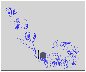
Figure 1 shows a sketch that defines an oscillating circular cylinder near a plane boundary, where the size of the cylinder is exaggerated relative to the fluid domain size in order to see the detail of the configuration. The cylinder oscillates translationally about a mean position  $O$ with an amplitude of
  $A$ and a direction angle
  $\unicode[STIX]{x1D6FD}$ measured from the plane boundary. The diameter of the cylinder is
  $D$ and minimum gap between the cylinder and plane boundary when the cylinder is at its lowest position is
  $G$. A local coordinate system
  $OXY$ is defined with its origin located at the mean position of the cylinder and the
  $X$-direction aligned in the oscillation direction of the cylinder and pointing away from the plane boundary. The displacement of the cylinder is expressed as
 $$\begin{eqnarray}X=A\sin (\unicode[STIX]{x1D714}t),\end{eqnarray}$$
 where  $A$ is the amplitude of the oscillation,
  $\unicode[STIX]{x1D714}=2\unicode[STIX]{x03C0}/T$,
  $T$ is the oscillation period and
  $t$ is time; the position of the cylinder centre on the
  $oxy$ coordinate system is
  $x=X\cos (\unicode[STIX]{x1D6FD})$ and
  $y=y_{0}+X\sin \unicode[STIX]{x1D6FD}$, where
  $y_{0}=G+D/2+A\sin \unicode[STIX]{x1D6FD}$ is the mean vertical position of the cylinder centre. Angles
  $\unicode[STIX]{x1D6FD}=0^{\circ }$ and
  $90^{\circ }$ correspond to the cases where the cylinder oscillates horizontally and vertically, respectively. The oscillatory velocity of the cylinder in the
  $X$-direction is
  $U_{c}=U_{m}\cos (\unicode[STIX]{x1D714}t)$, where
  $U_{m}=\unicode[STIX]{x1D714}A$ is the amplitude of the oscillatory velocity, and its components in the
  $x$- and
  $y$-directions are expressed as
  $U_{c}\cos (\unicode[STIX]{x1D6FD})$ and
  $U_{c}\sin (\unicode[STIX]{x1D6FD})$, respectively.

Figure 1. Definition sketch of an oscillating cylinder near a plane boundary in quiescent fluid. The maximum and minimum positions in the  $X$-direction are marked as two circles.
The fluid flow relative to the cylinder for the configuration shown in figure 1 is different from oscillatory flow past a stationary cylinder in the following two aspects. Firstly, the cylinder can oscillate in different directions in figure 1, instead of only in the horizontal direction. Secondly, if a cylinder oscillates near a plane boundary, the flow relative to the cylinder is a uniform flow with a velocity of  $u_{F}=-U_{c}$, which does not vary spatially in the fluid domain. The boundary layer flow on the plane boundary does exist because, relative to the cylinder, the fluid and the plane boundary move simultaneously with a same speed. If a cylinder is placed in an oscillatory flow on a plane boundary, the external flow is boundary layer flow and the flow pattern is affected by the boundary layer thickness (Carstensen, Sumer & Fredsøe Reference Carstensen, Sumer and Fredsøe2010; Xiong et al. Reference Xiong, Cheng, Tong and An2018).
This study is relevant to hydrodynamics around subsea pipelines and mooring lines in offshore oil and gas engineering and heat and mass transfer in thermal and fluid engineering. Offshore riser pipes and mooring lines are important facilities and they are connected to floating oil and gas platforms. The motion of a floating platform due to ocean waves forces riser pipes and mooring lines to oscillate. At the sea bottom, the flow induced by the oscillation can cause erosion of the sediment near the pipelines and mooring lines. In this study, two-dimensional numerical simulations are conducted to investigate the flow induced by an oscillating cylinder near a plane boundary for a constant low Reynolds number of 150. The effects of the  $KC$ number and the gap between the cylinder and the plane boundary on the flow patterns are discussed in detail.
Two-dimensional simulations are conducted at a relatively low Reynolds number and low  $KC$ numbers, considering the affordability of a detailed study over a wide parametric space and acceptable accuracy of two-dimensional numerical simulations. Through direct numerical simulations, Nehari, Armenio & Ballio (Reference Nehari, Armenio and Ballio2004) reported that the three-dimensionality of the flow does not have effects on the two-dimensional features. Specifically, the V-shaped vortex shedding pattern of regime D and the diagonal vortex shedding pattern of regime F are inherent features of two-dimensional flow caused by two-dimensional instability. In the experimental studies, the length of the cylinder should be sufficiently long, and end plates were used to minimize the effects from the two ends of the cylinder (Sarpkaya Reference Sarpkaya2002). As a result, these vortex flow patterns can be simulated using two-dimensional numerical models. It was also reported that three-dimensionality has little influence on the hysteresis effect at low to intermediate
  $KC$ and Stokes numbers. Because three-dimensionality is weak at relatively low
  $Re$ and low
  $KC$, the flow structures and fluid force can be well predicted by two-dimensional numerical models (Justesen Reference Justesen1991; Dütsch et al. Reference Dütsch, Durst, Becker and Lienhart1998; Zhao & Cheng Reference Zhao and Cheng2014; Tong et al. Reference Tong, Cheng, Zhao and An2015).
2 Numerical method
The governing equations for solving the flow in the computational domain shown in figure 1 are the incompressible two-dimensional Navier–Stokes (NS) equations. The computational domain deforms continuously if the cylinder oscillates. To account for the deformation of the computational domain, the NS equations are solved using the arbitrary Lagrangian–Eulerian (ALE) scheme. In the ALE scheme, the computational mesh nodes move based on the updated position of the cylinder in every computational time step. The mesh nodes can be moved in an arbitrary way that minimizes the distortion of the computational mesh. The coordinates  $(x,y)$, the velocity
  $(u,v)$, the time
  $(t)$ and the pressure
  $(p)$ are non-dimensionalized as
  $(x,y)=(x^{\prime },y^{\prime })/D$,
  $(u,v)=(u^{\prime },v^{\prime })/U_{m}$,
  $t=U_{m}t^{\prime }/D$ and
  $p=p^{\prime }/(\unicode[STIX]{x1D70C}U_{m}^{2})$, respectively, where the prime stands for dimensional values. The non-dimensional NS equations can then be written as
 $$\begin{eqnarray}\displaystyle & \displaystyle \frac{\unicode[STIX]{x2202}u_{i}}{\unicode[STIX]{x2202}t}+(u_{j}-\hat{u} _{j})\frac{\unicode[STIX]{x2202}u_{i}}{\unicode[STIX]{x2202}x_{j}}=-\frac{\unicode[STIX]{x2202}p}{\unicode[STIX]{x2202}x_{i}}+\frac{1}{Re}\unicode[STIX]{x1D6FB}^{2}u_{i}, & \displaystyle\end{eqnarray}$$
 $$\begin{eqnarray}\displaystyle & \displaystyle \frac{\unicode[STIX]{x2202}u_{i}}{\unicode[STIX]{x2202}x_{i}}=0, & \displaystyle\end{eqnarray}$$
 where  $x_{1}=x$ and
  $x_{2}=y$,
  $u_{i}$ is the velocity in the
  $x_{i}$-direction,
  $\hat{u} _{i}$ is the non-dimensional moving velocity of the computational mesh in the
  $x_{i}$-direction and
  $Re$ is the Reynolds number defined as
  $Re=U_{m}D/\unicode[STIX]{x1D708}$, where
  $\unicode[STIX]{x1D708}$ is the kinematic viscosity of the fluid. The non-dimensional oscillation period of the cylinder is defined as the Keulegan–Carpenter (
 $KC$) number:
 $$\begin{eqnarray}KC=U_{m}T/D.\end{eqnarray}$$
 The relationship between  $KC$ number and the oscillation amplitude is
  $KC=2\unicode[STIX]{x03C0}A/D$.
In the rest of the paper, all the variables are non-dimensional unless specifically stated otherwise. The length and height of the non-dimensional computational domain are 100 and 70, respectively, and the mean position of the cylinder is at the centre of the domain in the horizontal direction. The blockage when the cylinder oscillates in the horizontal direction is 1.4 %. Anagnostopoulos & Minear (Reference Anagnostopoulos and Minear2004) reported that, for the calculation of the fluid force of a cylinder in an oscillatory flow, the blockage effect is almost negligible if it is less than 20 %. The blockage used in this study is much smaller than 20 % to ensure the propagation of vortex streets will not be affected by the boundaries of the computational domain.
The NS equations are solved by the finite element method (FEM) model and the computing code developed by Zhao et al. (Reference Zhao, Cheng, Teng and Dong2007). In the FEM model, the stable Petrov–Galerkin method proposed by Brooks & Hughes (Reference Brooks and Hughes1982) is used to solve the NS equations. The numerical model has been validated against various scenarios with low Reynolds numbers in the laminar flow regime, including oscillatory flow past circular cylinders (Zhao & Cheng Reference Zhao and Cheng2014) and vortex-induced vibration (VIV) of circular cylinders (Zhao, Cheng & Zhou Reference Zhao, Cheng and Zhou2013; Zhao & Yan Reference Zhao and Yan2013). The validation of the numerical model has not been repeated in this paper.
When VIV of cylinders in a uniform flow is studied using the ALE scheme, the deformation of the mesh was calculated by solving the modified Laplace equation (Zhao & Yan Reference Zhao and Yan2013)
 $$\begin{eqnarray}\unicode[STIX]{x1D735}\boldsymbol{\cdot }(\unicode[STIX]{x1D6FE}\unicode[STIX]{x1D735}S_{i})=0,\end{eqnarray}$$
 where  $S_{i}$ is the displacement of the mesh nodes in the
  $x_{i}$-direction and
  $\unicode[STIX]{x1D6FE}$ is a constant that controls the mesh deformation, which is inversely proportional to the area of a finite element. However, it is difficult to maintain mesh quality using (2.4) when the gap between the cylinder and the plane boundary is extremely small. To avoid over-distortion of finite elements, the mesh movement scheme used in this study is similar to that used by Rahmanian et al. (Reference Rahmanian, Cheng, Zhao and Zhou2014). For each combination of
  $KC$ number and
  $G$, two predefined structured meshes are generated, one with the minimum possible gap and one with the maximum possible gap between the cylinder and the plane boundary, as shown in figure 2(a) and (b), respectively. The two meshes have exactly the same structures, node numbers and node number indices. When the cylinder is between the minimum and maximum positions, the coordinates of all the nodes are calculated using an interpolation method. By using the above method, the mesh quality will always be as good as the ones shown in figure 2.

Figure 2. Computational mesh for  $KC=5$ when the cylinder is at its (a) highest and (b) lowest positions.
Both the cylinder surface and the plane boundary are smooth walls and the boundary conditions are specified as follows. A non-slip boundary condition is given on the smooth-wall boundaries. Specifically, the fluid velocity is the same as the velocity of the cylinder’s motion on the cylinder surface and zero on the plane boundary. On the two side and top boundaries, the flow velocity is zero and the pressure is zero. The gradient of the pressure in the normal direction of the boundary on the plane boundary and the cylinder surface is zero.
The computational domain is divided into 102 152 and 184 136 four-node quadrilateral elements for  $G=0.1$ and 4, respectively. The mesh number increases with the increase of
  $G$ because the number of elements between the cylinder and the plane boundary increases. The cylinder surface is divided into 128 elements and the mesh size in the radial direction on the cylinder surface is 0.002. The density of the mesh used in this study is denser than that used in Zhao & Cheng (Reference Zhao and Cheng2014), where a detailed mesh dependence study was conducted for oscillatory flow past two cylinders at
  $Re=100$ and 150.
To demonstrate that the computational domain size of  $100\times 70$ is sufficiently large to obtain converged results, an extra calculation with
  $G=0.1$ and
  $KC=12$ (the maximum
  $KC$ number used in this study) is simulated using a computational domain with a size of
  $200\times 140$. Figure 3(a) shows the comparison between the non-dimensional forces from the two meshes and figure 3(b) shows the comparison of horizontal fluid velocities along three horizontal lines of
  $y=0.1$, 0.6 and 1.1. The non-dimensional lift forces are defined as
  $C_{X}=F_{X}/(\unicode[STIX]{x1D70C}DU_{m}^{2}/2)$ and
  $C_{Y}=F_{Y}/(\unicode[STIX]{x1D70C}DU_{m}^{2}/2)$, where
  $F_{X}$ and
  $F_{Y}$ are the forces in the
  $X$- and
  $Y$-directions, respectively. Both forces and the fluid velocities from the larger domain size are nearly identical to their counterparts from the smaller domain size. The velocity oscillates in the horizontal direction mainly because of the wake vortices, which will be discussed in detail in the next section.

Figure 3. Comparison between the results from two meshes with different domain sizes for  $G=0.1$ and
  $KC=12$.
3 Vortex flow patterns
3.1 Oscillation of a cylinder without a plane boundary
Flow induced by an oscillating cylinder in the horizontal direction in quiescent fluid without a plane boundary is first simulated and the results are used as a benchmark to evaluate how the plane boundary affects the flow. According to the regime map proposed by Tatsuno & Bearman (Reference Tatsuno and Bearman1990), regimes  $\text{A}^{\ast }$, A, D and F can be found for
  $Re=150$ and
  $KC$ in the range of 1–12. Streaklines at the time when
  $Y=0$ and
  $U_{c}=-U_{m}$ are shown in figure 4 to identify flow patterns. Throughout the paper, all the streaklines are generated by releasing massless particles at 80 points evenly distributed along the circle outside the cylinder with a non-dimensional radius of 0.51. In each case, a series of velocity fields with a time interval of
  $T/32$ are used to generate the streaklines.
Regimes  $\text{A}^{\ast }$ and A are characterized by progression of particles in two opposite directions in a straight line. Although no vortex shedding occurs and there is no vortex street in either regime
  $\text{A}^{\ast }$ or regime A, the massless particles move away from the cylinder, leaving a street of streaklines on each side of the cylinder. The flow streets presented by the streaklines are referred to as streakline streets in this study. The difference between regime
  $\text{A}^{\ast }$ and A is that vortices are formed in regime A but not in regime
  $\text{A}^{\ast }$. However, there is not a distinct boundary between regimes
  $\text{A}^{\ast }$ and A (Tatsuno & Bearman Reference Tatsuno and Bearman1990). The flow is in regime
  $\text{A}/\text{A}^{\ast }$ for
  $KC=2$ to 5, where two streakline streets are symmetrically located on two sides of the cylinder, and regime D for
  $KC=6$ and 7, where one pair of vortices are shed from only one side of the cylinder in one oscillation period. The streaklines for
  $KC=6$ in figure 4(e) show a vortex being shed from the top side of the cylinder as the cylinder moves left.
The flows for  $KC=9$ to 12 are in regime F, where two pairs of vortices are shed from the cylinder in one vibration period. The vortex pairs can be clearly identified in the streaklines of regime F in figure 4(f–h), and they propagate away from the cylinder. The alignment angles of the streakline streets in regime F for different
  $KC$ numbers are different. The two streakline streets are aligned nearly in the horizontal direction at
  $KC=9$, aligned diagonally with a small inclination angle at
  $KC=10$ and approximately
  $45^{\circ }$ inclination angle at
  $KC=12$. The regimes B, E and G are not discussed in this study, because they occur at high Reynolds numbers
  $(Re>200)$, where the flow is strongly three-dimensional. Based on the vortex numbers that are shed from the cylinder in one oscillation period, regimes D and F were also classified as single- and double-pair regimes, respectively (Williamson Reference Williamson1985).

Figure 4. (c–h) Flow streaklines for an oscillating cylinder in the horizontal direction without a plane boundary for  $Re=150$. The time histories and the frequency spectra of the lift coefficient are shown in (a) and (b), respectively.
Figure 4(a,b) shows the time histories and frequency spectra calculated by the fast Fourier transform of the non-dimensional lift force, respectively. In regime D, one pair of vortices is shed from the cylinder in one period and vortices are only shed from one side of the cylinder. If the side where vortices are shed changes intermittently, the regime was also named as regime E (Tatsuno & Bearman Reference Tatsuno and Bearman1990). For  $KC=7$ in figure 4(a) the change of negative mean lift coefficient during
  $t/T=45$ to 80 to positive mean lift force during
  $t/T=80$ to 120 is due to the switch of the vortex shedding from one side of the cylinder to the other side. The switch of the vortex shedding side of the cylinder was also found through both two- and three-dimensional numerical simulations (Lin, Bearman & Graham Reference Lin, Bearman and Graham1996; Uzunoglu, Tan & Price Reference Uzunoglu, Tan and Price2001; Nehari et al. Reference Nehari, Armenio and Ballio2004). The frequency spectra in figure 4(b) shows that the non-dimensional frequency
  $f_{Y}T$ of the highest peak of the lift force equals the vortex shedding pair number plus 1 (Williamson Reference Williamson1985). The very irregular oscillation of lift force for
  $KC=8$ in figure 4(a) indicates that the flow is transitioning from regime D to F. The component of
  $f_{Y}T=3$ is higher than that of
  $f_{Y}T=2$ in the frequency spectrum for
  $KC=8$ in figure 4(b), indicating that the flow is dominated by regime F. Flows for
  $KC=9$ to 12 are periodic regime F flows judged by the very periodic oscillation of the lift force in figure 4(a).
3.2  $G=0.1$ and $0.5$


The results for  $G=0.1$ and 0.5 are discussed separately in this section because such gaps have significant effects on the vortex shedding flow. Flow patterns for
  $G=0.1$ and
  $\unicode[STIX]{x1D6FD}=0^{\circ }$,
  $45^{\circ }$ and
  $90^{\circ }$ are discussed in detail. Flow patterns for
  $G=0.5$ and
  $\unicode[STIX]{x1D6FD}=0^{\circ }$ are discussed at the end of this section, while flows of
  $G=0.5$,
  $\unicode[STIX]{x1D6FD}=45^{\circ }$ and
  $90^{\circ }$ are not discussed in detail because they share the same patterns as those for
  $G=0.1$. Figure 5 shows the time histories of the non-dimensional force
  $C_{Y}$ for
  $G=0.1$ and
  $\unicode[STIX]{x1D6FD}=0^{\circ }$,
  $45^{\circ }$ and
  $90^{\circ }$. Figure 6 shows streaklines when the cylinder is moving in the positive
  $X$-direction through its mean position (
 $X=0$ and
  $U_{c}=U_{m}$) for
  $G=0.1$. The periodic oscillation of the force in figure 5 indicates that the repeatability of the flow is very good. If
  $G=0.1$ and the oscillation direction is horizontal (
 $\unicode[STIX]{x1D6FD}=0^{\circ }$), vortices are found to generate only from the top side of the cylinder. All the streaklines for different
  $KC$ numbers shown in figure 6(a) are in the shape of a rotated C pattern. The density of the streaklines near the cylinder decreases with the increase of
  $KC$ number, because the speed of particles moving away from the cylinder increases. The dominant frequency of the lift coefficient is 2 for
  $\unicode[STIX]{x1D6FD}=0^{\circ }$ for all the
  $KC$ numbers because two maximum lift coefficients was created during one oscillation period.

Figure 5. Time histories and frequency spectra of the non-dimensional force in the  $Y$-direction for
  $G=0.1$: (a)
  $\unicode[STIX]{x1D6FD}=0^{\circ }$, (b)
  $\unicode[STIX]{x1D6FD}=45^{\circ }$ and (c)
  $\unicode[STIX]{x1D6FD}=90^{\circ }$. The dashed horizontal grid lines are
  $C_{Y}=0$ lines and the spacing between these lines is 4.
All the streakline patterns in figure 6(a) are in a rotated C shape. To observe the motion of vortices, figure 7(a) shows the contours of vortices corresponding to the cases in figure 6(a). The vortex flow patterns for  $G=0.1$ and
  $KC=4$ and 5 are in regime A where vortex shedding does not occur and vortex streets do not exist. As regards
  $KC=4$, the vortex generated from the cylinder in one half-cycle is convected back to the other side of the cylinder after the cylinder’s motion changes its direction and dissipates quickly. In figure 7(b), the positive vortex A is nearly fully grown before the cylinder’s velocity becomes zero and changes its direction. The reversal of the cylinder makes vortex A go back to the right side, instead of being shed from the cylinder. Because every vortex generated from one side of the cylinder moves to another side before it has enough size to be shed form the cylinder, no vortex shedding is observed in regime A.

Figure 6. Streaklines when the cylinder is moving in the positive  $X$-direction through its mean position for
  $G=0.1$.
At  $KC=9$ two vortices are shed from the cylinder (vortices A and B in figure 7c) in one period and the vortex shedding is in mode D. Vortex
  $\text{B}^{\ast }$ is shed from the cylinder in the previous cycle. After each vortex is shed from one side of the cylinder, it is convected back to the opposite side, escapes from the cylinder and then moves away from the cylinder horizontally, resulting in one well-defined vortex street on either side of the cylinder. Vortex A, as an example, which is shed from the left side of the cylinder at
  $t/T=0.25$, is convected back to the right side at
  $t/T=0.5$ and continues to move towards the right direction and joins the right vortex street. The vortex shedding remains in mode D until
  $KC=12$. Regime F vortex shedding, where two pairs of vortices are shed from the cylinder in one period, is not observed because the extremely small gap does not allow vortices to be generated from the bottom side of the cylinder. When vortices move horizontally away from the cylinder, shear layers were generated between them and the plane boundary, which are in the opposite directions of vortices. The strong vortices near the cylinder attract the fluid towards them, resulting in C-shaped streakline streets.
With the increase of  $KC$, the vortices travel for a longer time in one oscillation period while the number of vortices generated in one period remains the same, and as a result the distance between two neighbouring vortices (defined as
  $\unicode[STIX]{x1D706}$ in figure 7) in each regime D vortex street increases. The
  $\unicode[STIX]{x1D706}$ value can only be identified from the vorticity contours if
  $KC\geqslant 7$ because vortices do not move away from the cylinder at smaller
  $KC$ numbers. The variation of
  $\unicode[STIX]{x1D706}$ with the non-dimensional amplitude of the cylinder
  $A/D~(=KC/2\unicode[STIX]{x03C0})$ is shown in the middle of figure 7, and it can be seen that
  $\unicode[STIX]{x1D706}$ increases nearly linearly with the increase of
  $A/D$. For
  $KC=12$, vortices move along the plane boundary for a distance before their direction biases upwards. Regime D vortex shedding for
  $G=0.1$ is similar but not exactly the same as that for oscillatory flow around a stationary cylinder for
  $G=0.25$ and
  $KC=11$ observed in figure 12 in Xiong et al. (Reference Xiong, Cheng, Tong and An2018), where an extra pair of small vortices is shed from the cylinder in one period. In the study of oscillation flow past a stationary cylinder by Xiong et al. (Reference Xiong, Cheng, Tong and An2018), the two vortex streets remain moving horizontally along the plane boundary instead of rolling up. When a cylinder oscillates horizontally along a plane boundary in a still fluid, no boundary layer flow exists and the two vortex streets separate from the boundary, forming a rotated C-shaped vortex flow pattern as shown in figure 7(d).

Figure 7. Contours of vorticity at four instants of  $t/T=0$, 0.25, 0.5 and 0.75 within one period for
  $G=0.1$ and
  $\unicode[STIX]{x1D6FD}=0^{\circ }$. The variation of the vortex-to-vortex distance
  $\unicode[STIX]{x1D706}/D$ with the oscillation amplitude
  $A/D$ of the cylinder is presented at the centre of the figure.
In figure 5, the zero-lift lines are marked as dashed grid lines. It can be seen that the mean lift forces for  $\unicode[STIX]{x1D6FD}=0^{\circ }$ and
  $G=0.1$ are all positive. In figure 5(a), the mean lift force is slightly greater than zero as
  $KC=2$ and increases significantly as
  $KC=3$. As
  $KC$ exceeds 4, the lift coefficient remains positive in nearly a whole oscillation period.
The fluid flow caused by the cylinder motion is expected to be strong near the cylinder and negligibly weak far away from the cylinder. Figure 8 shows the profiles of the horizontal velocity  $u$ along different vertical lines at
  $t/T=0$ and 0.5 (where the cylinder’s velocity is 1 and
  $-1$, respectively) for
  $G=0.1$,
  $\unicode[STIX]{x1D6FD}=0^{\circ }$ and two
  $KC$ numbers. Under the nonslip boundary condition, the velocity is zero at
  $y=0$ and the same as the velocity of the cylinder on the cylinder surface
  $(x-X,y)=(0.5,0.6)$. When the cylinder’s velocity reaches its maximum in the positive
  $x$-direction, the fluid velocities along the lines of
  $x-X=0.5$ to 8 are smaller than the cylinder’s velocity
  $(u=1)$. When the cylinder is moving in the negative
  $x$-direction and reaches its maximum velocity
  $(u=-1)$, the fluid velocities near the cylinder centre in figure 8(d) for
  $KC=9$ are greater than the cylinder velocity. The high velocity is between the negative vortex B and the positive vortex below it shown in figure 7(c). Owing to the inertia effect, the phases of the fluid velocities below the cylinder’s top surface level is ahead of those above the cylinder.
For a sinusoidal oscillatory flow on a plane boundary, the non-dimensional boundary layer thickness is  $\unicode[STIX]{x1D6FF}=(3\unicode[STIX]{x03C0}/4)\sqrt{KC/\unicode[STIX]{x03C0}Re}$ (Carstensen et al. Reference Carstensen, Sumer and Fredsøe2010), which are marked in figure 8. The boundary layer flow driven by the oscillatory cylinder is only confined within a thin layer of fluid close to the plane boundary. If the boundary layer thickness is defined as the height where the velocity reaches its maximum value, its values at difference horizontal locations are different from each other in figure 8. The
  $\unicode[STIX]{x1D6FF}$ value is less than 0.5 close to the cylinder (
 $x=0.5$ to 2) and much greater than
  $D$ far away from the cylinder where the velocity is small, for example at
  $x=8$.

Figure 8. Profiles of velocity  $u$ along vertical lines at different locations for
  $G=0.1$,
  $\unicode[STIX]{x1D6FD}=0^{\circ }$ and
  $KC=5$ and 9.

Figure 9. Contours of vorticity at four instants of  $t/T=0$, 0.25, 0.5 and 0.75 within one period for
  $G=0.1$ and
  $\unicode[STIX]{x1D6FD}=45^{\circ }$.
When the cylinder vibrates diagonally with  $\unicode[STIX]{x1D6FD}=45^{\circ }$, the streaklines on the right side of the cylinder are similar to those of an isolated cylinder without a plane boundary, while those on the left side are significantly altered (see figure 6b). When
  $KC=4$, 5 and 6, no streakline street is observed at the left side of the cylinder as shown in figure 6(b). When
  $KC=9$ and 12, the plane boundary forces the vortex street on the left side of the cylinder to roll up and form a recirculation region. Figure 9 shows contours of vorticity at four instants of
  $t/T=0$, 0.25, 0.5 and 0.75 within one period for
  $G=0.1$ and
  $\unicode[STIX]{x1D6FD}=45^{\circ }$. Since the characteristics of the vortex street on the top of the cylinder are the same as those on one side of an isolated cylinder, the vortex shedding modes can be classified according to the top branch streakline street. When the cylinder moves diagonally upwards, the increasing gap between the plane boundary and the cylinder allows vortices to be generated, and the vortex generation mechanism from the bottom side of the cylinder is the same as that from the top side. For
  $KC=4$ and 5, the generation of the two vortices from the bottom side of the cylinder at
  $t/T=0.25$ and the motion of these two vortices towards the top side before they are shed due to the reversal of the cylinder are typical phenomena of the regime A flow pattern. The asymmetry of the configuration of the flow causes net lift force in regime A in figure 5(b) but with a much smaller amplitude than that for
  $\unicode[STIX]{x1D6FD}=0^{\circ }$ for the same
  $KC$.
$KC$.
In regime D in figure 9(d), one vortex A is shed from the bottom side of the cylinder as the cylinder reaches its highest position at  $t/T=0.25$. The diagonally upward motion of the cylinder makes enough gap between the cylinder and the plane boundary to allow vortices to grow and shed from the cylinder in regime D. However, the vortices below the cylinder dissipate quickly due to the effect of the plane boundary. In regime D, the vortex street on the top side of the cylinder includes positive and negative vortices generated from the top and bottom of the cylinders, respectively. It is similar to that of an isolated cylinder because the negative vortices that are shed from the bottom side of the cylinder (for example, vortex A in figure 9c,d) are convected to the top side before they are affected by the plane boundary. Compared with that in regime A, the lift coefficient in regime D is significantly increased because vortices are only generated at one side of the cylinder.
In regime F in figure 9(e,f), two vortices are shed from the cylinder in each half-period. Two vortices (A or C) remain on the side of the cylinder where they are shed, and the two vortices (B or D) are convected back to the opposite side of the cylinder after they are shed. The alignment angle of the vortex street in regime F for an isolated cylinder varies with  $KC$ as shown in figure 4; so does that in the case with a plane boundary with
  $\unicode[STIX]{x1D6FD}=45^{\circ }$. The vortex street from the top side of the cylinder is not affected by the plane boundary if it is aligned diagonally upwards (figure 9e,f), and is attracted towards the boundary if it is aligned nearly horizontally (figure 9g). As a result, in figure 9(g), negative vortices dissipate quickly, leaving a row of positive vortices in the right vortex street at
  $KC=12$. The vortex shedding patterns for
  $\unicode[STIX]{x1D6FD}=45^{\circ }$ were not observed in either the case of flow past two cylinders (Zhao & Cheng Reference Zhao and Cheng2014) or the case of oscillation flow past a cylinder near a plane boundary (Xiong et al. Reference Xiong, Cheng, Tong and An2018).
In regime A and  $\unicode[STIX]{x1D6FD}=90^{\circ }$, the lower branch streakline street splits into two equal halves after it attacks the plane boundary, resulting in a perfectly symmetric flow as shown in figure 6(c) and a zero-lift coefficient as shown in figure 5(c). The splitting of the lower branch streakline street results in one recirculation region at each side of the cylinder. Comparing figure 6(b) with figure 6(c) it can be seen that regimes D and F vortex flow patterns for
  $\unicode[STIX]{x1D6FD}=90^{\circ }$ are similar to those in the same regimes for
  $\unicode[STIX]{x1D6FD}=45^{\circ }$. This is mainly because the vortex street below the cylinder is aligned diagonally for both oscillation directions, although the motion of the cylinder is not inclined for
  $\unicode[STIX]{x1D6FD}=90^{\circ }$. In regimes D and F, the diagonally aligned lower branch streakline street rolls up and forms a recirculating region after it meets the plane boundary. At
  $KC=9$ in figure 6(c), the lower branch streakline street meets the boundary nearly vertically and forms a small recirculation zone at the right side of the cylinder. At
  $KC=12$, the lower branch streakline street approaches the plane boundary at an inclined angle, and it forms a larger recirculation region. The vorticity contours for
  $\unicode[STIX]{x1D6FD}=90^{\circ }$ in figure 10 for each flow regime are similar to those for the same regime for
  $\unicode[STIX]{x1D6FD}=45^{\circ }$ in figure 9, except for regime A.
Based on the streaklines in figure 6, it is expected that the fluid motion around the cylinder can cause strong period-averaged mean velocity, which is generally referred to as steady streaming (Sumer & Fredsøe Reference Sumer and Fredsøe2001; An, Cheng & Zhao Reference An, Cheng and Zhao2009). Steady streaming is one of the mechanisms for mass and heat transfer in a fluid. The steady streaming streamlines for some representative cases for  $G=0.1$ are shown in figure 11. To understand the formation mechanisms of the steady streaming, the contours of the mean pressure coefficient are plotted in figure 11. The mean pressure coefficient is defined as
  $\overline{C}_{p}=\overline{p}/(\unicode[STIX]{x1D70C}U_{m}^{2}/2)$, where the overbar stands for averaged value over one oscillation period of the cylinder. The low pressure near the cylinder is caused by the vortices generated by the separated shear layers. The recirculating regions formed by the streamlines in figure 11 correlate well with the streaklines shown in figure 6. The streamline concentration areas in figure 11 are where the streakline streets are.

Figure 10. Contours of vorticity for  $\unicode[STIX]{x1D6FD}=90^{\circ }$ and
  $G=0.1$ when the cylinder is at its highest position (upper row) and its lowest position (lower row).
At  $\unicode[STIX]{x1D6FD}=0^{\circ }$, the motion of the cylinder creates high pressure below the cylinder and at the left and right sides of the cylinder, which generates strong horizontal flow velocities directing away from the cylinder along the plane boundary. The low pressure above the cylinder attracts the streamlines and makes them bend towards the cylinder. The rolling up of the vortex streets is also the result of the suction effect of the low-pressure zone above the cylinder. At
  $\unicode[STIX]{x1D6FD}=0^{\circ }$, the two recirculating zones on the two sides of the cylinder are formed by the rolling up of the two streakline streets. As the
  $KC$ number increases from 5 to 12, the centres of the recirculating zones move away from the cylinder. The steady streaming streamlines for
  $\unicode[STIX]{x1D6FD}=0^{\circ }$ are perfectly symmetric and the centre of each recirculation zone is measured by coordinates
  $X$ and
  $Y$ defined in figure 12. It can be seen that the centre of each recirculation zone does not move further away from the cylinder as
  $KC$ is increased from 9 to 12, indicating that the distance of a horizontal vortex street travelling along the plane boundary does not increases.
In regime A of  $\unicode[STIX]{x1D6FD}=45^{\circ }$ and
  $90^{\circ }$, low pressure is only confined in a small area near the two sides of the cylinder because vortex shedding does not happen and vortices do not travel away from the cylinder. As a result, the steady streaming flow converges towards the cylinder from its two sides and leaves the cylinder from the top side. In regime A, the high pressure in the small area below the cylinder generates horizontal steady streaming flow on each side of the cylinder and a recirculating zone is formed after this type of steady streaming meeting the converging flow towards the cylinder (see figure 11e,f). In figure 11(e), only one small recirculation zone is formed on the left side of the cylinder because the high pressure only occurs at the left side. In figure 11(f), the high pressure immediately below the cylinder centre forms two recirculation zones on two sides of the cylinder.

Figure 11. Streamlines and contours of pressure coefficient based on the period averaged flow for  $G=0.1$.
If the gap between the cylinder and the plane boundary is small, the oscillation of the cylinder creates strong shear stress on the plane boundary and causes erosion if the plane boundary is erodible. A typical example of boundary erosion is the erosion of the seabed sediment around vibrating pipelines in subsea engineering. The capacity of erosion can be evaluated by the non-dimensional shear stress defined as  $\unicode[STIX]{x1D70F}=(1/Re)\,\unicode[STIX]{x2202}u/\unicode[STIX]{x2202}y$, where
  $\unicode[STIX]{x2202}u/\unicode[STIX]{x2202}y$ is the non-dimensional gradient of the horizontal velocity on the plane boundary. Figure 13 shows the distribution of the maximum shear stress
  $\unicode[STIX]{x1D70F}_{max}$ along the plane boundary for
  $G=0.1$, where
  $\unicode[STIX]{x1D70F}_{max}$ at a location is defined as the maximum
  $|\unicode[STIX]{x1D70F}|$ within one oscillation period of the cylinder. Generally,
  $\unicode[STIX]{x1D6FD}=0^{\circ }$ causes much higher
  $\unicode[STIX]{x1D70F}_{max}$ than
  $\unicode[STIX]{x1D6FD}=45^{\circ }$ and
  $90^{\circ }$ because the cylinder remains close to the plane boundary throughout the whole period. For
  $\unicode[STIX]{x1D6FD}=0^{\circ }$, the smallest
  $KC$ number of 2 produces the largest
  $\unicode[STIX]{x1D70F}_{max}$ but the smallest high
  $\unicode[STIX]{x1D70F}_{max}$ region. Large acceleration of the cylinder and the fluid velocity at a small
  $KC$ number creates strong flow velocity locally in a small region. As a result, the shear stress on the plane boundary is increased locally. The area of high
  $\unicode[STIX]{x1D70F}_{max}$ region increases with the increase of
  $KC$ number because the distance that the cylinder can reach increases. The distribution of
  $\unicode[STIX]{x1D70F}_{max}$ along the plane boundary is perfectly symmetric as
  $G=0.1$ and
  $\unicode[STIX]{x1D6FD}=0^{\circ }$.
As  $\unicode[STIX]{x1D6FD}$ is increased from
  $0^{\circ }$ to
  $45^{\circ }$, the increased averaged gap between the cylinder and plane boundary results in a significant reduction in
  $\unicode[STIX]{x1D70F}_{max}$. The maximum
  $\unicode[STIX]{x1D70F}_{max}$ is located at the left side of the cylinder. When the cylinder moves diagonally downwards, it drives the fluid to flow diagonally and attack the plane boundary, resulting in much higher
  $\unicode[STIX]{x1D70F}_{max}$ on the left side of the cylinder than on the right side. The diagonally downward motion of the streamlines at the left side of the cylinder is correlated to the diagonal motion of the vortices in figure 9.

Figure 12. Positions of the centres of the recirculation zones of the streaming for  $G=0.1$ and
  $\unicode[STIX]{x1D6FD}=0^{\circ }$.
As  $\unicode[STIX]{x1D6FD}$ is further increased to
  $90^{\circ }$,
  $\unicode[STIX]{x1D70F}_{max}$ is further reduced and its distribution along the plane boundary is symmetric only when the flow is in regime
  $\text{A}^{\ast }/\text{A}$ in the range of
  $KC=2$ to 5. At
  $KC=6$ and above, the
  $\unicode[STIX]{x1D70F}_{max}$ distribution is asymmetric because of the intrinsic asymmetric flow in regimes D and F. From figure 13(c) it can be seen that, in regimes D and F, the side of the cylinder towards which the lower branch vortex street biases has wider high
  $\unicode[STIX]{x1D70F}_{max}$ zone than its opposite side. However, the largest
  $\unicode[STIX]{x1D70F}_{max}$ values on both sides of the cylinder appear not to be significantly different from each other. Based on the above discussion, it can be concluded that horizontal oscillation of the cylinder causes most capacity of erosion of the plane boundary by the flow and the vertical motion causes least for a very small gap of
  $G=0.1$. For all three angles of
  $\unicode[STIX]{x1D6FD}=0^{\circ }$,
  $45^{\circ }$ and
  $90^{\circ }$, the maximum shear stress occurs at the smallest
  $KC$ number, but the widest high-shear-stress region occurs at the largest
  $KC$ number.

Figure 13. Distribution of maximum shear stress along the plane boundary for  $G=0.1$.
Figure 14 shows the distribution of period-averaged mean shear stress ( $\overline{\unicode[STIX]{x1D70F}}$) along the plane boundary for
  $G=0.1$. The maximum mean shear stress on the plane boundary for
  $\unicode[STIX]{x1D6FD}=0^{\circ }$ decreases and its location moves away from the cylinder with the increase of the
  $KC$ number. For
  $\unicode[STIX]{x1D6FD}=45^{\circ }$ and
  $90^{\circ }$, the distribution of
  $\overline{\unicode[STIX]{x1D70F}}$ on the plane boundary is highly asymmetric except for the case of regime A for
  $\unicode[STIX]{x1D6FD}=90^{\circ }$. The common feature of the mean stress of most of the cases is that it is zero at a point either below or somewhere near the cylinder centre, and directs away from this zero point at the two sides. If the plane boundary was an erodible sandy seabed and the cylinder was a subsea pipeline, this feature would make sediment move away from the zero-mean-shear-stress point and leave a scour pit there.

Figure 14. Distribution of mean stress along the plane boundary for  $G=0.1$.

Figure 15. Streaklines and vortex contours for  $G=0.5$ and
  $\unicode[STIX]{x1D6FD}=0^{\circ }$.
The vortex shedding flow regimes observed for  $G=0.5$ and
  $\unicode[STIX]{x1D6FD}=45^{\circ }$ and
  $90^{\circ }$ are similar to those for
  $G=1$ and the same oscillation directions. The vortex shedding flows for
  $G=0.5$ and
  $\unicode[STIX]{x1D6FD}=0^{\circ }$ shown in figure 15 show some distinct differences from those for
  $G=0.1$ and
  $\unicode[STIX]{x1D6FD}=0^{\circ }$. As the gap increases from 0.1 to 0.5, vortices are generated from the bottom side of the cylinder and they are stronger than those from the top side. As a result, regime A streakline streets are originated from the bottom side of the cylinder in figure 15(a). The flow pattern for
  $KC=6$ and
  $G=0.5$ is in regime D with two vortices being shed from the cylinder in one vibration period, which are labelled as vortices A and B, respectively, in figure 15(f). It is interesting to see in figure 15(b) that the massless particles for generating streaklines move around the cylinder only within a small area. An extremely small number of particles escape from the top side of this small area and, as a result, no streakline streets are formed. Why particles are trapped in figure 15(b) can be explained by observing the motion of vortices around the cylinder in figure 15(f). After vortex A is shed from the cylinder, it circles around the cylinder to the right side and merges into a negative vortex. In the second half-period, vortex B is shed from the cylinder and repeats exactly what vortex A does. The vortices generated from the top side of the cylinder also merge into other vortices; for example, vortex C merges into B. The circulating of the vortices around the cylinder results in a featureless streaklines pattern without any streets shown in figure 15(b). Regime F occurs when
  $KC=9$ and 12 (see figure 15g,f), where two vortices A and B are shed from the cylinder before the cylinder reaches it maximum displacement at
  $t/T=0.25$ and another two vortices C and D are shed from the cylinder at
  $t/T=0.75$. In figure 15(g), vortices A and
  $\text{D}^{\ast }$ (the star means this vortex was generated in the previous period) combine and vortices B and C combine. Because of the combination of vortices, the pattern of the streakline streets in regime F of
  $G=0.5$ are similar to that in regime D of
  $G=0.1$.

Figure 16. Time histories of the non-dimensional lift force for  $G=1$ and 4. The horizontal dashed grid lines are the
  $C_{Y}=0$ lines.
3.3 $G=1$, $2$ and $4$


In this section the flow structures for  $G=1$, 2 and 4 are discussed together because they share similar characteristics. Regimes A, D and F are discussed separately. Figure 16 shows time histories of the non-dimensional lift force for all the simulated cases with
  $G=1$ and 4. Compared with those for
  $G=0.1$, the oscillation of many lift forces is aperiodic, indicating that flow does not repeat from period to period. It can be seen that aperiodicity of the lift force mainly occurs at
  $KC=6$ and 7, where the flows are in regime D and
  $KC=8$, which is the boundary between regimes D and F. In regime D, vortex shedding only occurs at one side of the cylinder. However, the vortex shedding may change from one side of the cylinder to the other side intermittently. This has been observed both in experimental studies (Tatsuno & Bearman Reference Tatsuno and Bearman1990) and in numerical simulations (Nehari et al. Reference Nehari, Armenio and Ballio2004). The change of the vortex shedding side of the cylinder in regime D makes the mean lift coefficient change its direction intermittently in figure 16. It appears that the lift force in regime F (
 $KC=9$ to 12) does not vary between one period and another except for
  $\unicode[STIX]{x1D6FD}=0^{\circ }$ and
  $G=1$, indicating that the flow pattern is fixed. For
  $G=1$ and
  $KC=9$ to 12, the lift force is aperiodic because vortices that are shed from the bottom side of the cylinder are deformed significantly when they go through the very narrow gap with the flow. The detailed wake flow structure will be discussed later on. The lift coefficient in regime A for
  $\unicode[STIX]{x1D6FD}=0^{\circ }$ and
  $\unicode[STIX]{x1D6FD}=45^{\circ }$ decreases dramatically as
  $G$ increases from 0.1 to 1 and beyond. In figure 16,
  $C_{Y}$ is nearly zero for
  $KC=2$ and 3 and all the oscillation directions, and is only weakly visible as
  $KC=4$ and 5 and
  $\unicode[STIX]{x1D6FD}=0^{\circ }$ and
  $\unicode[STIX]{x1D6FD}=45^{\circ }$.

Figure 17. Streaklines for regime A when the cylinder is moving upwards through its mean position for  $G=1$, 2 and 4. The arrows indicate the direction of travel of the vortex street.
Figure 17 shows the streaklines of regime  $\text{A}^{\ast }/\text{A}$ for different
  $G=1$, 2 and 4 and some representative
  $KC$ numbers. At
  $\unicode[STIX]{x1D6FD}=0^{\circ }$, streakline streets for the two regimes
  $\text{A}^{\ast }/\text{A}$ are generated from the two sides of the cylinder. They bend towards the plane boundary due to the attraction by the shear layers on top of the plane boundary, which are indicated in the vorticity contours in figure 18. After each streakline street meets the plane boundary, it is divided into two streets: one moves towards the cylinder and another moves away. A recirculated streakline street is formed on each side of the cylinder. As the gap is increased to 4, each streakline street propagates at a very small speed before it meets the plane boundary and very small percentage of streakline particles move towards the cylinder thereafter. The symmetric flow pattern for
  $\unicode[STIX]{x1D6FD}=0^{\circ }$ is similar to half of regime A–A or
  $\text{A}^{\ast }$–
 $\text{A}^{\ast }$ flow pattern for oscillatory flow past two side-by-side cylinders (Zhao & Cheng Reference Zhao and Cheng2014) but not exactly the same. Geometrically, the plane boundary is equivalent to the symmetry line in the streamwise direction for oscillatory flow past two side-by-side cylinders. However, for flow past two side-by-side cylinders, the symmetry line dividing the two cylinders is equivalent to a symmetric boundary with free-slip boundary condition, while in this study, the plane boundary is a non-slip boundary.

Figure 18. Contours of vorticity for regime A when the cylinder is moving in the positive  $X$-direction through its mean position for
  $G=1$, 2 and 4.
If the cylinder oscillates vertically in regime  $\text{A}/\text{A}^{\ast }$, the flow becomes perfectly symmetric about the vertical symmetry line. Each regime
  $\text{A}/\text{A}^{\ast }$ flow for
  $\unicode[STIX]{x1D6FD}=90^{\circ }$ has two branches of streaklines: the branch above the cylinder is not affected and the branch below is divided into two by the plane boundary. After the division, each half-lower-branch streakline street rolls up and forms a recirculation zone. Before it attacks the plane boundary, the vortex
  $\text{A}/\text{A}^{\ast }$ streakline street can be clearly identified when
  $G$ is equal to and greater than 1. For
  $\unicode[STIX]{x1D6FD}=90^{\circ }$, the regime A flow for all the gaps is perfectly symmetric because the perfect symmetric streakline street below the cylinder enables it to be evenly divided into two halves after it meets the plane boundary.
By observing figure 17, one can see that, if a streakline street meets the plane boundary, it tends to roll up and form (a) recirculation streakline street(s), instead of moving along the boundary, especially in the case of  $\unicode[STIX]{x1D6FD}=0^{\circ }$ and
  $90^{\circ }$. If a vortex attacks the plane boundary at nearly a right angle of attack, it splits into two halves and each half only has vortices in one direction. The low pressure caused by vortices with the same vorticity sign in a vortex street attracts the flow towards the vortices and forms a recirculation zone. The flow structure for
  $G=2$ is similar to that in figure 6(b) in Xiong et al. (Reference Xiong, Cheng, Tong and An2018), where oscillatory flow past a circular cylinder is studied. In the configuration of
  $\unicode[STIX]{x1D6FD}=0^{\circ }$, if flow relative to the cylinder is examined, both the fluid and the plane boundary oscillate simultaneously in the horizontal direction and the relative free-stream velocity (the undisturbed velocity without the cylinder) is a uniform flow without a boundary layer. As a result, as indicated in figure 18, the motion of the cylinder only creates shear layers with strong vorticity locally near the cylinder. In figure 7(b) by Xiong et al. (Reference Xiong, Cheng, Tong and An2018), who studied oscillatory flow past a cylinder on a plane boundary, the surface of the whole plane boundary is covered by a strong shear layer because the undisturbed flow is a boundary layer flow.
The mechanisms of streakline street bending towards the plane boundary for  $\unicode[STIX]{x1D6FD}=0^{\circ }$ is the same as that of two parallel vortex streets of two side-by-side cylinders attracting each other reported by Zhao & Cheng (Reference Zhao and Cheng2014). The blockage effect increases the velocity of the fluid relative to the cylinder in the gap, making the vortices below the cylinder centre stronger than those above. The unevenness of the vortices can be clearly seen in figure 18 and it makes the streakline streets bend downwards. In addition, the shear layers generated above the plane boundary also attract the streakline street downwards. At
  $\unicode[STIX]{x1D6FD}=90^{\circ }$ the lower branch regime A and
  $\text{A}^{\ast }$ vortex street in the streakline (figure 17) is evenly divided into two halves by the plane boundary for all the studied gaps including
  $G=0.1$. The size of each recirculation zone below the cylinder increases with the increase of the gap ratio.
The regime A vortex flow on the left side of the cylinder for  $\unicode[STIX]{x1D6FD}=45^{\circ }$ has similar characteristics to that for
  $\unicode[STIX]{x1D6FD}=0^{\circ }$, i.e. the streakline street attacks the plane boundary at an inclined angle and divides into two halves. After division, the part that moves towards the right direction is negligibly smaller than that moving left and it is negligibly weaker when
  $G=1$. The right branch of the streakline street for
  $\unicode[STIX]{x1D6FD}=45^{\circ }$ bends towards the plane boundary after it travels for some distance.
From figure 18 it can be seen that, for  $\unicode[STIX]{x1D6FD}=0^{\circ }$ and
  $90^{\circ }$, shear layers on the surface of the plane boundary are generated below the cylinder and they are in opposite directions relative to the two vortices above them. The attraction between the two shear layers on the plane boundary and the two vortices above them contributes to the bending of the streaklines towards the wall for
  $\unicode[STIX]{x1D6FD}=0^{\circ }$.
3.4 Regime D
Figure 19 shows the streaklines and contours of vorticity for regime D with  $G=1$, 2 and 4. In figure 19(a), the streakline street pattern at the left side of the cylinder is similar to regime A flow, while the vortex flow at the right side of the cylinder is typical of regime D. The combined regimes A and D flow pattern was defined as regime AD (Zhao & Cheng Reference Zhao and Cheng2014). Regime D for
  $G=2$ and 4 and
  $\unicode[STIX]{x1D6FD}=0^{\circ }$ is the same as that for an isolated cylinder without a plane boundary. In regime D, vortex shedding only occurs from the gap side of the cylinder as
  $G=1$ because the stronger flow velocity through the gap than that above the cylinder generates stronger vortices. For the same reason, vortices are only shed from the bottom side of the cylinder in regime D for
  $\unicode[STIX]{x1D6FD}=45^{\circ }$ and
  $G=1$. At
  $G=4$, the effect of the plane boundary has been very weak and the vortex shedding is found to switch between the top and bottom sides of the cylinder intermittently. Regime D vortex shedding is affected by the plane boundary the most when
  $\unicode[STIX]{x1D6FD}=90^{\circ }$, where the lower branch streakline street always forms a recirculation region after it meets the plane boundary. The reason why a regime D streakline street tends to form one recirculation zone instead of two after it meets the plane boundary is that each vortex street is dominated by vorticities in one direction. The direction of the recirculation zone formed by a vortex street is always the same as the direction of the dominant vortices in the vortex street.

Figure 19. Streaklines and contours of vorticity for regime D with  $G=1$, 2 and 4.
Figure 20 shows vorticity contours and streaklines for  $G=1$ and
  $KC=9$. The two vortices A and B labelled in figure 20 are shed from the cylinder at
  $t/T=0.25$ and 0.75, respectively. After the cylinder motion changes its direction, they move through the gap to the opposite side of the cylinder (see figure 20b,d), which is typical behaviour of vortices in regime D. After a vortex moves from one side to another side of the cylinder through the gap, its strength is reduced significantly because the gap is very small. In addition, the remnant of vortices B and A moves around instead of away from the cylinder. As a result, no regime D streakline street is found. The vorticity contours and streaklines in figure 20 has strong similarity with those of regime D in figure 15(b,f). The flow in figure 20 is treated as regime D flow because the number of the vortices that are shed from the cylinder in one oscillation period and the motion of the vortices after they are shed are the same as those regime D.

Figure 20. Vorticity contours and streaklines of regime D for  $G=1$ and
  $KC=9$.
3.5 Regime F
Figure 21 shows vorticity contours and streaklines when the cylinder moves through its mean position in the positive  $X$-direction for
  $KC=9$ and 12 and
  $G=1$, 2 and 4. Regime F vortex shedding patterns can be clearly identified except in figure 21(a,d), where the gap between the cylinder and the plane boundary is 1. The flow in figure 21(a) is in regime D, which has been shown in detail in figure 20. The flow in figure 21(d) is in regime F, where two pairs of vortices shed from the cylinder in one cycle are marked in the vorticity contour diagram. Apart from those in figure 21(b,d), the vortex shedding process of the regime F flow is the same as that for an isolated cylinder without a plane boundary shown in figure 4. However, after vortices are shed from the cylinder, their motion is affected by the boundary in different ways in different cases.

Figure 21. Streaklines and contours of vorticity for  $KC=9$ and 12 with
  $G=1$, 2 and 4.
At  $KC=9$ and
  $\unicode[STIX]{x1D6FD}=0^{\circ }$, three recirculation zones (marked by arrows in figure 21) are observed in streaklines. The right streakline street bends downwards and splits into two after it attacks the plane boundary, and then forms two recirculation zones with very different sizes. The curved left branch streakline street forms the third recirculation zone. For
  $KC=12$ and
  $\unicode[STIX]{x1D6FD}=0^{\circ }$, the upper branch streakline also bends downwards. However, it forms only one recirculation zone instead of two because it does not split into two branches after it reaches the plane boundary. In regime F flow for
  $G=1$ and
  $KC=12$, the pair of vortices at the lift side of the cylinder do not propagate far from the cylinder due to the effect of the plane boundary. When the flow is in the positive
  $x$-direction, this pair of vortices is squeezed through the small gap. The timing of this vortex pair going through the small gap is different from period to period, leading to aperiodic flow. As a result, the lift coefficient on the cylinder is aperiodic as shown in figure 16. The regime F streaklines for
  $\unicode[STIX]{x1D6FD}=45^{\circ }$ are also in the three-recirculation-zone pattern for both
  $KC=9$ and 12, because the lower branch streakline always attacks the plane boundary nearly vertically.
For  $\unicode[STIX]{x1D6FD}=90^{\circ }$ in figure 21, while the upper branch regime F streakline is not affected by the plane boundary, the behaviour of the lower branch streakline depends on the
  $KC$ number. When
  $KC=9$, both branches of streaklines are nearly perpendicular to the plane boundaries. As a result, the lower branch attacks the plane boundary and splits into two. For
  $KC=12$, the lower branch streakline approaches the plane boundary with an inclined angle and forms a single recirculation zone.
4 Classification of the flow regimes
After the flow patterns of all the simulated cases are examined, a refined flow classification method specifically for an oscillatory cylinder close to a plane boundary is proposed. In the above discussion, the regimes are named following the definition by Tatsuno & Bearman (Reference Tatsuno and Bearman1990). In the absence of the plane boundary, each of the flow regimes A, D and F has two streakline streets. The plane boundary changes these streakline streets mainly in the following five possible ways:
(i) One street disappears totally when the gap between the cylinder and the plane boundary is very small.
(ii) There are still two streakline streets, one or both form recirculated street(s).
(iii) One streakline street is divided into two after it attacks the plane boundary at nearly a right angle.
(iv) Both streakline streets are divided into two after they meet the plane boundary, resulting in four branches of streakline streets.
(v) Streaklines circle around the cylinder, leaving no streakline streets.
To further differentiate the behaviour of streakline streets, variant numbers 0 to 4 are added to the flow regime names A, D and F to represent the number of streakline streets. For example, the flows for  $KC=4$, 5 and 6 in figure 6(b) are in regimes A1 and D1, respectively, because there is only one streakline street; the flows for
  $KC=9$ and 12 in figures 6(b) and 21(e,f) are in regime F2, because two streakline streets are seen; the flows in figure 21(i,n) are in regime F3 since one of the vortex streets is divided into two, resulting in three vortex streets in total; the flows in figure 17(a–c) are in regime A4 because both streakline streets are divided into two branches; and the flows in figures 15(b) and 20 are in regime D0, because no streakline streets are found. In regime F, the variants of the flow regimes can be identified by both vortex streets and streaklines because there is strong vortex shedding. In regimes
  $\text{A}^{\ast }/\text{A}$ and D, the variants of the flow regimes can only be identified through streaklines because vortex streets presented by vorticity contours either do not exist or are too weak.

Figure 22. Flow regime mapping on the  $KC$–
$KC$– $G$ plane.
Based on the above flow classification method, all the calculated cases are mapped on the  $G$–
$G$– $KC$ plane in figure 22. Because there is not a well-defined boundary between A and
  $\text{A}^{\ast }$ (Tatsuno & Bearman Reference Tatsuno and Bearman1990), the regimes A and
  $\text{A}^{\ast }$ are together on the maps. On the maps, some examples from the figures are given for each regime. In the absence of the plane boundary, the ranges of
  $KC$ numbers for regimes
  $\text{A}/\text{A}^{\ast }$, D and F are
  $2\leqslant KC\leqslant 5$,
  $6\leqslant KC\leqslant 7$ and
  $8\leqslant KC\leqslant 12$, respectively. It can be seen that the plane boundary does not change the
  $KC$ range of regime
  $\text{A}/\text{A}^{\ast }$ significantly but does affect the variant of the regime. Regime F is not observed at
  $\unicode[STIX]{x1D6FD}=0^{\circ }$ and
  $G=0.1$ because vortices are only generated from the top side of the cylinder. Regime
  $\text{A}^{\ast }4/\text{A}4$ only occurs as
  $\unicode[STIX]{x1D6FD}=0^{\circ }$, where both streakline streets on the two sides of the cylinder are already on the plane boundary after they form. All the oscillation angles have large areas of F3 on the map, because the vertically and diagonally downward propagation of the streakline street below the cylinder provides a great chance of streakline street splitting after attacking the plane boundary. Regimes D0 and
  $\text{A}^{\ast }4/\text{A}4$ only occur when
  $\unicode[STIX]{x1D6FD}=0^{\circ }$.
5 Force coefficients
When a cylinder is placed in an oscillatory flow, the fluid force in the streamwise direction approximately follows the Morison equation (Bearman et al. Reference Bearman, Downie, Graham and Obasaju1985), which is expressed as
 $$\begin{eqnarray}F_{X}(t)=\frac{1}{2}\unicode[STIX]{x1D70C}DC_{D}|u_{F}(t)|u_{F}(t)+\unicode[STIX]{x1D70C}\frac{\unicode[STIX]{x03C0}D^{2}}{4}C_{M}\frac{\text{d}u_{F}(t)}{\text{d}t},\end{eqnarray}$$
 where  $F_{X}$ is the fluid force acting on the cylinder in the positive
  $X$-direction,
  $u_{F}(t)=-U_{c}$ is the velocity of the quiescent fluid relative to the oscillating cylinder, and
  $C_{M}$ and
  $C_{D}$ are inertia and drag coefficients, respectively. The inertia and drag coefficients for all the simulated cases are obtained using the least-squares method based on 20 periods of data and presented in figure 23. To examine the applicability of the Morison equation in the case of a cylinder close to a plane boundary, the coefficients of determination
  $R^{2}$ for the fitted coefficients
  $C_{M}$ and
  $C_{D}$ are shown in figure 23(g–i). The coefficient of determination is defined as
 $$\begin{eqnarray}R^{2}=1-\mathop{\sum }_{n=n_{0}+1}^{n_{0}+mN}(F_{X,n,Morison}-F_{X,n})^{2}\!\left/\mathop{\sum }_{n=n_{0}+1}^{n_{0}+mN}F_{X,n}^{2},\right.\end{eqnarray}$$
 where  $F_{x,n}$ and
  $F_{X,n,Morison}$ are the forces at the
  $n$th computational time step calculated by numerical simulations and Morison equation, respectively,
  $n_{0}$ is the starting time step when the vibration has been stabilized,
  $N$ is the time step within one oscillation period of the cylinder and
  $m=20$.
If there were no plane boundary, the inertia coefficient would increase with increase of  $KC$ in regime
  $\text{A}/\text{A}^{\ast }$, and decrease in regimes D and F. The irregular variation of the drag coefficient in regime D in the
  $KC$ range between 6 and 8 is because of the intermittent change of the flow patterns. It can be seen that the smallest gap of
  $G=0.1$ significantly increases both inertia and drag coefficients for all three oscillation directions, and the maximum and minimum increments occur at
  $\unicode[STIX]{x1D6FD}=0^{\circ }$ and
  $90^{\circ }$, respectively. By observing the regime mapping in figure 22 and the force coefficient in figure 23, it can be seen that all the inertia and drag coefficients within one flow regime generally vary with
  $KC$ with similar trends except for
  $G=0.1$. For example, with the increase of
  $KC$, all coefficients except for
  $G=0.1$ in figure 23(c) increase in regime
  $\text{A}/\text{A}^{\ast }$, change irregularly in regime D and decrease in regime F. At
  $\unicode[STIX]{x1D6FD}=0^{\circ }$ and
  $G=0.1$, the inertia coefficient increases and the drag coefficient decreases with increasing
  $KC$ as
  $KC>6$ because the flow is consistently in regime D.

Figure 23. Inertia and drag coefficients for the Morison equation.
As  $G$ exceeds 1, the effect of
  $G$ on
  $C_{M}$ is weaker in regime
  $\text{A}^{\ast }/\text{A}$ than in other regimes because vortices in this regime are mainly confined near the cylinder and do not have much interaction with the plane boundary. The inertia coefficient
  $C_{M}$ for
  $G=4$ is very close to that of a cylinder without a plane boundary, except in regime D, indicating that the influence of the gap on the force has been very weak. The maximum difference between the drag coefficients with and without a plane boundary is found to be in regime A. Once
  $G=1$ and above, the drag coefficient is only weakly affected by the plane boundary. The difference between
  $C_{D}$ with
  $G=1$ and that without a plane boundary is within 10 % for all the
  $KC$ numbers. From figure 23(g–i) it can be seen that
  $R^{2}$ of the Morison equation is very close to 1 in regime A, especially at
  $G\geqslant 1$. It reduces with the increase of
  $KC$ but is still above 0.92 at the largest
  $KC=12$ and the smallest
  $G=0.1$.
Figure 24 shows the variation of the standard derivation (SD) of the lift coefficient  $C_{Y}^{\prime }$ with the
  $KC$ number. The SD of the lift coefficient of one oscillation period is calculated numerically as
  $C_{Y}^{\prime }=\sqrt{(1/N)\sum _{n=n_{0}+1}^{n_{0+N}}(C_{Y,n}-\overline{C}_{Y})^{2}}$, where
  $C_{Y,n}$ is the
  $C_{Y}$ at the
  $n$th computational time step,
  $n_{0}$ is the starting time step where the flow has been stabilized and
  $\overline{C}_{Y}$ is the time-averaged value of
  $C_{Y}$. In cases where the flow pattern changes intermittently, the statistical values of the lift coefficient vary significantly with time as shown in figure 16. For these cases, the SD of the lift coefficient of each oscillation period is calculated and the mean value of the top 10 % periods with the highest
  $C_{Y}^{\prime }$ is shown in figure 24. For
  $\unicode[STIX]{x1D6FD}=90^{\circ }$,
  $C_{Y}^{\prime }=0$ in regime A because the flow is perfectly symmetric. For
  $\unicode[STIX]{x1D6FD}=0^{\circ }$ and
  $45^{\circ }$,
  $C_{Y}^{\prime }$ is nearly zero if
  $G$ is greater than 2. In all the gap ratios, the maximum
  $C_{Y}^{\prime }$ is found to occur in regime D (
 $KC$ between 6 and 8) and the effect of the gap on
  $C_{Y}^{\prime }$ is strongest in regime D. The effect of the plane boundary on
  $C_{Y}^{\prime }$ for
  $\unicode[STIX]{x1D6FD}=90^{\circ }$ is the weakest and that for
  $\unicode[STIX]{x1D6FD}=0^{\circ }$ is the strongest.

Figure 24. Variation of the standard derivation (SD) of the lift coefficient with the  $KC$ number.
6 Conclusions
Flow induced by an oscillating cylinder close to a plane boundary at a low Reynolds number of 150, oscillating direction angles of  $\unicode[STIX]{x1D6FD}=0^{\circ }$,
  $45^{\circ }$ and
  $90^{\circ }$, and
  $KC=2$ to 12 is investigated by numerical simulations. The main conclusions are summarized as follows.
For an extremely small gap of  $G=0.1$ and
  $\unicode[STIX]{x1D6FD}=0^{\circ }$, regime F disappears because no vortices are generated or shed from the bottom side of the cylinder. For
  $G=0.1$ and
  $\unicode[STIX]{x1D6FD}=45^{\circ }$ and
  $90^{\circ }$, the vortex shedding is the same as that of a cylinder without a plane boundary; however, one streakline street in regimes
  $\text{A}^{\ast }/\text{A}$ and D is suppressed because of the strong effect from the plane boundary. In addition, the lower branch streakline street of regime F forms a recirculation zone. The very small gap ratio of
  $G=0.1$ creates a large shear stress on the plane boundary, especially at
  $\unicode[STIX]{x1D6FD}=0^{\circ }$.
The vortex shedding processes for  $G=1$, 2 and 4 are the same for a specific
  $KC$. However, the behaviour of the streakline street (or vortex street in regimes D and F) varies with
  $G$. If
  $\unicode[STIX]{x1D6FD}=90^{\circ }$, regime
  $\text{A}^{\ast }/\text{A}$ flow is always symmetric for all the simulated gaps. In regime D and
  $\unicode[STIX]{x1D6FD}=0^{\circ }$ and
  $45^{\circ }$, vortices are only shed from the bottom of the cylinder if
  $G\leqslant 2$, and can change between the top and bottom of the cylinder intermittently if
  $G=4$. In regime F, if the lower branch of the vortex street attacks the plane boundary at nearly a right angle of attack, it splits into two and forms two recirculation zones. If it diagonally approaches the plane boundary, it rolls up and forms one recirculation zone.
For a cylinder without a plane boundary, each flow regime has two streakline streets. Owing to the effect of the plane boundary, a streakline may disappear, bend and form a recirculation zone, or split into two streets after it attacks the plane boundary at nearly a right angle of attack. Because of the above process, the streakline street number could be either increased or decreased. To represent the behaviour of streakline streets after they are formed, the streakline street number is used as the variant number and added to each regime name proposed by Tatsuno & Bearman (Reference Tatsuno and Bearman1990). The identified refined regime names, which are the combination of regime name and variant number, are mapped on the  $KC$–
$KC$– $G$ plane. The
  $KC$ range for regime
  $\text{A}^{\ast }/\text{A}$ is not changed but the variant of regime
  $\text{A}^{\ast }/\text{A}$ is dependent on
  $KC$ and
  $\unicode[STIX]{x1D6FD}$. All variants 1 to 4 are found in regime A. Regimes D3 or D4 are never found because a regime D vortex street is dominated by vortices in a single direction, making it impossible to split into two streets with vortices with opposite signs. Regime F1 is not found because strong regime F vortex streets never disappear. Only one vortex street in regime F can split into two, and, as a result, regime F4 is not found.
The drag and inertia coefficients of the Morison equation are obtained using the least-squares method. A very small gap of  $G=0.1$ significantly increases both the drag and lift coefficients, especially when
  $\unicode[STIX]{x1D6FD}=0^{\circ }$. The effect of the plane boundary on the drag coefficient is less than 10 % compared with that of a cylinder without a plane boundary if
  $G=1$ and above. If
  $G=1$ and above, the effect of the plane boundary on the inertia coefficient is weak only in regime
  $\text{A}^{\ast }/\text{A}$. In regimes D and F, the effect of the plane boundary becomes weak as
  $G=4$.
Declaration of interests
The authors report no conflict of interest.


