


Introduction
Antarctic shags (Phalacrocorax (atriceps) bransfieldensis) are seabirds that feed on inshore demersal fish of the Southern Ocean. They breed in small colonies (mean colony size < 100 breeding pairs; Schrimpf et al. Reference Schrimpf, Naveen and Lynch2018) along the shore of the Antarctic Peninsula and surrounding islands. The colonies are located on rock outcrops and cliff tops where they build nests shaped like truncated cones. They lay up to three eggs in October–November and the eggs are incubated by both sexes (Shirihai & Kirwan Reference Shirihai and Kirwan2007).
A more detailed knowledge of shag populations could help in understanding the population dynamics of their prey species, which are otherwise hard to monitor (Casaux & Barrera-Oro Reference Casaux and Barrera-Oro2006, Harris et al. Reference Harris, Quintana, Ciancio, Riccialdelli and Raya Rey2016). Therefore, the Commission for the Conservation of Antarctic Marine Living Resources (CCAMLR) Ecosystem Monitoring Program (CEMP) included Antarctic shags as an indicator species of the Antarctic ecosystem for monitoring changes in coastal fish populations (CCAMLR 2014).
Surveys of Antarctic shags are rare as the birds breed at places that are remote and difficult to access along the shore of the Antarctic Peninsula. The birds at more than half (54%) of the known colonies of this species were last counted during or before the 1980s (Schrimpf et al. Reference Schrimpf, Naveen and Lynch2018). The common method of determining the size of shag colonies is by ground counts from vessels. However, with this method it is only possible to monitor a very limited number of colonies (Lynch et al. Reference Lynch, Naveen and Fagan2008, Casanovas et al. Reference Casanovas, Naveen, Forrest, Poncet and Lynch2015, Phillips et al. Reference Phillips, Silk, Massey and Hughes2019).
Aerial surveys are able to help increase the number of colonies that can be monitored. It is relatively common, for example, to use aerial images taken from helicopter, airplane or unmanned aerial vehicle (UAV) to assess the distribution and abundance of Antarctic penguin colonies (Pygoscelis spp.; Wilson et al. Reference Wilson, Pike, Southwell and Southwell2009, Southwell & Emmerson Reference Southwell and Emmerson2013, Goebel et al. Reference Goebel, Perryman, Hinke, Krause, Hann, Gardner and LeRoi2015, Borowicz et al. Reference Borowicz, McDowall, Youngflesh, Sayre-McCord, Clucas and Herman2018, Zmarz et al. Reference Zmarz, Rodzewicz, Dąbski, Karsznia, Korczak-Abshire and Chwedorzewska2018). However, such studies of shag colonies are very rare.
Colonies of sub-Antarctic shags like the New Zealand king shag (Leucocarbo carunculatus) and the Auckland Island shag (Phalacrocorax colensoi) have been surveyed using planes or helicopters (Schuckard et al. Reference Schuckard, Melville and Taylor2015). In Antarctica so far, only the population sizes of the colonies at Turret Point (King George Island) and Harmony Point (Nelson Island) have been determined by UAV surveys (Korczak-Abshire et al. Reference Korczak-Abshire, Zmarz, Rodzewicz, Kycko, Karsznia and Chwedorzewska2019, Oosthuizen et al. Reference Oosthuizen, Krüger, Jouanneau and Lowther2020). However, the positions of all these colonies were known before, and therefore it was not necessary to focus on colony characteristics or how to identify these colonies.
Detecting and quantifying shag colonies that were either unknown or those for which there is only vague spatial information using only aerial imagery has not yet been investigated. And vague spatial information is all that exists for most shag colonies in Antarctica. We therefore investigated whether it is possible to detect such colonies based solely on UAV images.
Shag nests with their bowled shape and the extensive guano cover surrounding the nests are unlikely to be confused with the nests of other species of flying birds breeding in the Antarctic. The nests of these other birds are much flatter and their surroundings less covered with guano (Mustafa et al. Reference Mustafa, Braun, Esefeld, Knetsch, Maercker, Pfeifer and Rümmler2019). However, it has not been analysed whether it is possible to distinguish shag nests from breeding penguins (both colonies are covered extensively by guano and adults have a similar appearance) nor how this might be done. These are important points because Antarctic shags often breed in, or close to, penguin colonies, as we show in this study.
The objectives of this study are:
• To identify all shag colonies in the study area.
• To identify and count of individual nests within colonies, including separation from chinstrap penguins where possible. This includes describing how the environmental conditions of the shag nesting areas differ from chinstrap penguins to help future UAV surveys of shags.
• To estimate changes in regional population size since the last surveys conducted in the 1980s.
Methods
Study area
The survey took place along a 30 km coastal section of north-western Nelson Island and south-western King George Island, South Shetland Islands, Antarctica (Fig. 1). The study area extended from Smilets Point (Nelson Island) in the south to Sygit Point (King George Island) in the north. The coast in the study area is characterized by hundreds of small ice-free islands and rocks. All of these are within 5 km of the coastline.
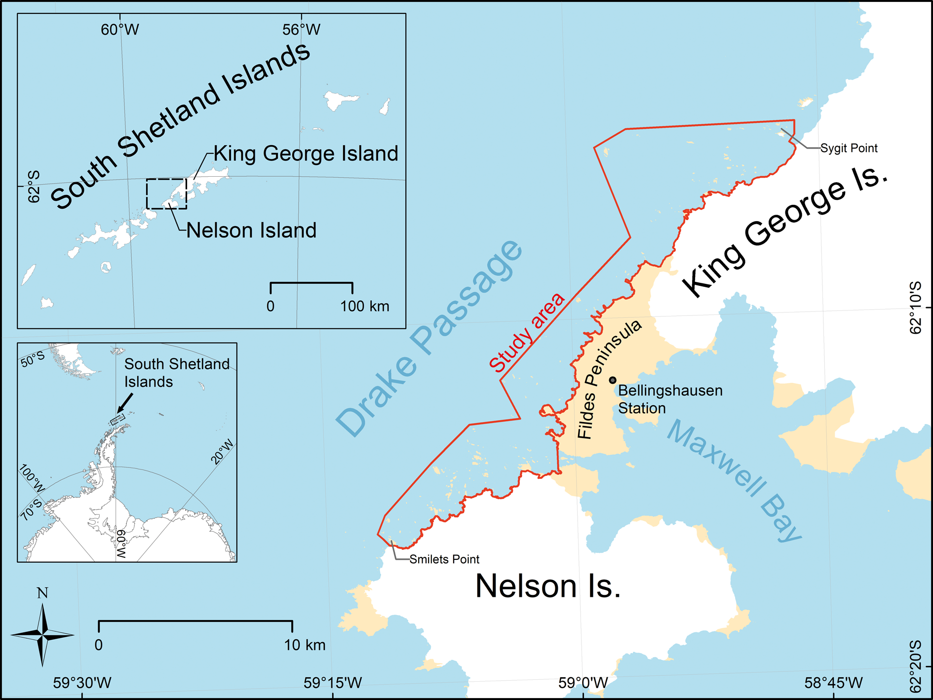
Fig. 1. The study area extended along the north-western coast of Nelson Island and the south-western coast of King George Island.
UAV flights and image processing
Between 11 December 2016 and 4 January 2017 we mapped all islands and rock outcrops in the survey area from an UAV. In this period, the shags were in the hatching phase. The flights were conducted with the electrically-powered delta fixed-wing UAV Bormatec Ninox which has a wing span of 1 m and a take-off weight of 1 kg (Fig. 2). We chose a fixed-wing UAV over the more commonly used multicopters for its greater range (Pfeifer et al. Reference Pfeifer, Barbosa, Mustafa, Peter, Rümmler and Brenning2019). The flight pattern was programmed pre-flight using the ground control station software Mission Planner v.1.3.40 (flight pattern downloadable in Pfeifer et al. Reference Pfeifer, Barbosa, Mustafa, Peter, Rümmler and Brenning2019). The flight height was 30–100 m above ground level (AGL), resulting in a ground sample distance (GSD) of 1–3.4 cm pixel-1. The colonies at Rzepecki Islands and Fregata Island were mapped twice in the season.

Fig. 2. The electrically-powered fixed-wing UAV “Ninox” used for the survey flights.
During the flights, the UAV was controlled fully autonomously by a Pixhawk 1 flight computer. This determined the position using the onboard IMU and a GNSS receiver. The airspeed was measured by a digital airspeed sensor. We equipped the UAV with a light weight (64 g) MAPIR Survey-2 RGB (16 megapixel) digital camera, taking images vertically downwards in JPG format every 2.5 seconds in manual exposure mode (f/2.8, shutter speed 1/500 s, ISO 50). The UAV was flying with an airspeed of 12 m s-1 up to 42 minutes per flight powered by two 2200 mAh (24.42 Wh) lithium polymer batteries. Long range flights with more than 15 km flight distance were only possible when the average wind speed was below 6 m s-1.
To be able to analyse the images from the UAV flights, we first stitched the single images and orthorectified the resulting mosaics (UTM21E/WGS84). For this we used the photogrammetry software Agisoft Photoscan Pro v.1.3 that uses structure from motion (SfM) techniques (Lowe Reference Lowe2004). During this process, a digital surface model (DSM) was also created for each orthomosaic. It was only possible to compute suitable very high-resolution DSMs (3.3–3.5 cm pixel-1) with images of Rzepecki Islands (flight from 30 December 2016) and of Kwarecki Point because only there the number of overlapping images was sufficient (> 6 images; McDowall & Lynch Reference McDowall and Lynch2017). For georeferencing, we used only the position of the UAV during camera exposure (saved in the Pixhawk log files), since no ground control points were available in the survey area. We therefore achieved an absolute XY-accuracy of < 10 m (see Pfeifer et al. Reference Pfeifer, Barbosa, Mustafa, Peter, Rümmler and Brenning2019). In total, 184 orthomosaics out of 14 027 images were created for analyses.
Identification of shag colonies
The orthomosaics were manually scanned for signs of bird colonies, namely guano covered ground or individual birds. Special attention was payed to areas near historically documented shag breeding sites and penguin colonies that appeared very similar to the shag colonies. This procedure was also applied to images that could not be stitched to an orthomosaic.
Colony characteristics
We defined the following characteristics of shag colonies and individuals in UAV imagery by analysing UAV-orthomosaics, single orthophotos and DSMs of the colonies with QGIS.
• For defining the topographic position of the colonies, the distance to the nearest cliff, the aspect and the height above the see level of the nests were defined with the help of UAV derived orthomosaics and DSMs..
• To quantify the differences in the visibility of the guano (see Rees et al. Reference Rees, Brown, Fretwell and Trathan2017) we used ENVI v.5.2 to calculate the Transformed Divergence (TD; Richards & Jia Reference Richards and Jia2006) of two class pairs (shag nest area and penguin nest area; shag nest area and rock without guano cover) in the UAV imagery of all colonies. The TD is a parametric separability index that indicates how well two classes statistically separate. The index ranges from 0 (no separability) to 2 (completely separable). The nest area of shags and penguins was obtained by calculating a buffer with 1 m radius around the centre of each shag nest or penguin individual. In addition to the TD the mean and the standard deviations for all three spectral bands of the UAV RGB images of the shag nest area, penguin nest area and rock, were calculated so as to also quantify changes in the visibility.
To find out if weather conditions affect the visibility of guano cover, we qualitatively compared the amount of precipitation in the seven days immediately before flights with the subjective visibility of the guano cover in the colonies as well as with the TD. The data on precipitation were recorded at the weather station of the Russian Antarctic Station Bellingshausen (see http://rp5.ru).
• The minimal nest distance was measured as the distance of each nest centre to the next closest nest centre. Nest diameter was measured manually for nests where the borders were well visible. Nests where edges were not visible were excluded from measurement.
• To determine the appearance of adults and chicks we looked for the typical characteristics described and displayed in exiting photographs (Shirihai & Kirwan Reference Shirihai and Kirwan2007) and compared them with the appearance in our UAV images. The characteristics we looked for were plumage colour, pattern of white on back, maximum visible body size and long neck. To get a general idea of appearance, we interpreted images showing individuals viewed from different angles of views and with different ground resolutions. Because the orthomosaic is usually stitched out of the centre parts of the images (near nadir looking), we also had to examine the edges of single orthophotos to get an oblique view of the birds.
• The ratio of adults and nests, in colonies that were separated from penguin colonies and the total number of adults within the guano covered areas was determined by counting all individuals that showed at least one characteristic feature of shag individuals. In colonies that were mixed with penguin nests, we counted only the number of adults detected by at least two observers, that were sitting on a clearly visible nest or that showed unique features of appearance.
Distinction of shag and penguin colonies
We also defined characteristics (the same as for shags) for chinstrap penguin colonies because counting shag nests was most difficult when these were close to or in between penguin nests. By comparing the characteristics defined in both species (i.e. guano colour, nest distance, appearance of adults) we were able to identify those characteristics which allowed us to distinguish between the two species in aerial imagery.
Breeding population size
If a shag colony was identified, the size of the population was determined by counting the number of nests using the characteristics described in the results. Counting was done using the GIS software QGIS v.2.18 (QGIS 2020), by visually interpreting the orthomosaics and single orthophotos showing the nest in question from different points of view. To enable spatial analysis, at the position of every nest, a point feature was placed in an ESRI shape-file. To account for individual-observer error in nest counts, all colonies were independently counted by three observers (CP, MR, OM). We then calculated the rounded up mean count as well as the range for every colony.
Changes in population size and distribution
To assess the long-term change in the numbers of occupied nests of each colony, we compared our counts with those of previous studies (Shuford & Spear Reference Shuford and Spear1988, Erfurt & Grimm Reference Erfurt and Grimm1990). Because Shuford & Spear (Reference Shuford and Spear1988) reported the census numbers of the shags as total number of adults, we divided the count by 1.5 as Schrimpf et al. (Reference Schrimpf, Naveen and Lynch2018) suggested, to estimate the total number of nests.
As the historic counts did not provide precise position data, we first had to locate the actual position of these colonies. If available, we used the assignment of the colonies to their possible actual location (Pfeifer et al. Reference Pfeifer, Barbosa, Mustafa, Peter, Rümmler and Brenning2019). The colony “#25” in Shuford & Spear (Reference Shuford and Spear1988) at the “Northwest side of Fildes Peninsula” (Shuford & Spear Reference Shuford and Spear1988) was assigned to the only current colony (“Unnamed Island-A”) in the area described. For the same reason, the count on one of the islands off Nelson Island, facing towards the “Drake side” (Erfurt & Grimm Reference Erfurt and Grimm1990), was assigned to Fregata Island. Table I summarises the assignments of the colonies we used in this study.
Table I. Assignment of the colony location of shag colonies where the precise position was not given by previous surveys.

a Translated to English
Results
Topographic colony position
Three of the four colonies detected were situated at the edge of, or overlapping with, chinstrap penguin colonies. All shag colonies detected were located at the highest north exposed parts of plateaus that are directly adjacent to cliffs (Fig. 3). These plateaus are 19–36 m above sea level.

Fig. 3. Three of the four colonies were located close to, or within, chinstrap penguin colonies. All Antarctic shag colonies were located at the highest north exposed parts of plateaus that are directly adjacent to cliffs.
Guano colour and visibility
Guano in shag colonies appears homogeneously white. The nests are enclosed by ring shaped areas (about 0.5–0.8 m radius), where the guano is brighter than in the surroundings. In the high-resolution images, single white guano lines radiating from the nests are visible. These guano rings are created when adults and chicks repeatedly squirt excrement in all directions while sitting on the nest. They are most visible at nests that are at the edges of colonies, or nests that are well separated from each other. At such positions, the neighbouring guano rings do not overlap, or mix, with the guano of passing penguins. At Rzepecki Islands, we found two guano rings without a nest inside indicating currently abandoned nest sites.
We noticed that the visibility of guano is not equal at all times. The guano in images of Fregata Island on 11 December 2016 is much more visible than in images from 20 December 2016, where the nest groups of shags and penguins are barely covered by guano and therefore hardly distinguishable from the surrounding rocks (Fig. 4a & b). The sparse guano cover of the nest groups on 20 December shows smaller differences in the mean brightness of the nest groups and the surrounding rocks measured in the RGB bands of the UAV images than on 11 December. While on 11 December the standard deviation (SD) of the brightness of the shag nest groups (n = 171 686 pixel) do not overlap with the penguin nest groups (n = 250 688 pixel) and the surrounding rocks (n = 225 029 pixel) in all three bands, they do on 20 December (Fig. 4c & d). Both values (mean brightness and SD) indicate a reduced visibility of the guano on 20 December. The same effect can be measured by the Transformed Divergence (TD) of the different class pairs (Table II). The TD of the shag nest groups and rock class was much higher on 11 December than on 20 December indicating a reduction in the spectral and statistical separability of both classes.
Table II. Comparison of the sum of precipitation three and seven days before the UAV flights, the subjective visibility of the guano and the Transformed Divergence (TD) for the shag and penguin nest groups as well as rock without guano. TD values > 1.9 indicate a good spectral separability of the class pairs.

a before date of flight
A comparison of the sum of precipitation three and seven days before the UAV flights and the visibility of the guano areas shows that weak visibility (20 December) was preceded by high precipitation (Table II).
Ratio of adults and nests
The results show changes of the ratio of adults to nests within the breeding season and from site to site (Table III). These ratios could not be determined for the colonies of Rzepecki Point and Kwarecki Point because these colonies are partially mixed up with breeding chinstrap penguins which prevented reliable distinction of adult shags and penguins.
Table III. The ratio of adults to nests changes within the breeding season and from site to site.

Spatial distribution of nests
The overall mean minimal distance (from centre to centre) between shag nests was 1.42 m (median = 1.24 m, interquartile range = 0.36 m, n = 106 shag nests; Fig. 5). The closest nest distances measured were at Rzepecki Islands (0.72 m) as was the furthest (6.7 m).

Fig. 4. In the UAV images, the guano cover of the nest groups of the colony on Fregata Island was a. more visible on 11 December than on b. 20 December. c. & d. Mean brightness in the RGB bands of Antarctic shag and chinstrap penguin nest groups and the guano free rocks with error bars indicating the standard deviation. c. On 11 December 2016 at Fregata Island the differences in the mean brightness of the Antarctic shag nest groups were greater than on d. 20 December for all bands.

Fig. 5. Histogram of the minimal nest distance of 106 Antarctic shag nest. The modal minimal distance between nests was 1–1.5 m.
The density of nests on guano covered areas was between 0.2 nests m-2 on “Unnamed Island-A” and 0.37 nests m-2 on Kwarecki Point (Table IV). At Kwarecki Point all shags were breeding in amongst a chinstrap penguin colony, making it impossible to determine separately the guano covered area of shags. At Rzepecki Islands, only the guano covered area of the part of the colony that was not mixed with the adjacent chinstrap penguin colony was included in the density calculation.
Table IV. Descriptive statistics (incl. standard deviation (SD) and interquartile range (IQR)) for the minimal nest distance and the density of nests on guano covered ground.

Appearance of nests
Shag nests are made out of clay/mud, plants, lichens as well as guano and in shape are a truncated cone or flattened mound. The nest edge appears as relatively bright rings around breeding adults or chicks. However, the nest edge was only visible for less than half of the nests. One or two adults were usually visible in the centre or the edge of the nest. The outer edge diameter of 43 shag nests borders had a mean of 49 cm (SD = 5 cm). Under cloud free conditions, shag nests cast a relatively big shadow that is easily visible (Fig. 6).

Fig. 6. Examples of a. & b. guano rings, c. & d. examples of nest shadows.
Because nests are apically bowl shaped, we were able to identify single nests from the UAV derived DSM (Fig. 7). This was only possible when the surroundings of the nests were flat and without smaller rocks, which lead to confusion with shag nests. However, the ground resolution of the DSM had to be very high (< 4 cm) to enable nest detection. But even with these DSMs, we were unable to detect nests reliably without a RGB orthomosaic due to artefacts caused by errors and noise during DSM creation. Using these DSMs, we determined nest heights of 10–40 cm (mean = 21.1 cm, SD = 9.9 cm, n = 16 nests). These measurements included the height of the nest itself and the bodies of the adults or chicks sitting in the nest. The body of the shags could only be reconstructed during DSM creation if they did not move during the acquisition of the overlapping images.

Fig. 7. a. & b. Shaded relief and RGB image showing the locations of two profiles of c. Antarctic shag and d. chinstrap penguin nests at Rzepecki Point made with a UAV derived DSM at a ground sample distance of 3.3 cm.
Appearance of adults and chicks
In the orthomosaics, we measured for 39 adults a mean maximum length of the visible body of 29 cm (SD = 8 cm) and mean maximum width of 17 cm (SD = 2 cm) in nadir view.
Adult shags are black-and-white with a predominantly black upper part and white underpart, which are visible from an oblique angle of view. In higher resolution images the rather prominent white upper back is visible as well as the black tail (around 4 cm wide). Shags have a long and thin neck that was particularly well recognizable in an oblique view e.g. on the edges of the image.
The chicks appeared entirely brown-black with no white and were only visible in orthomosaics from the end of December at the Rzepecki Islands. At this time they were not being brooded anymore and on some nests were starting to fledge. We were able to distinguish single fledgling chicks when they were sitting apart from each other outside the nest (Fig. 8). We were unable to distinguish single chicks when they were still lying closely packed in the nest. We were also unable to clearly distinguish between adults sitting close to each other.

Fig. 8. a. Adult Antarctic shag with clearly visible long neck, tail and white upper back. b. Adult Antarctic shag with three completely dark chicks next to a nest.
Other characteristics of shags like the beak colour or the yellow nasal caruncles could not be identified in the images.
Visibility of colony characteristics
All characteristic features of the individuals and nests have a relatively low detection rate (< 30%), with the exception of the nest shadow (detection rate > 80% if the sky is clear). We found that the visibility of the white lower back of adults, the long neck and the tail width correlated with the GSD of the orthomosaics (Fig. 9). These features were also visible in images with 3 cm GSD, but the probability of spotting them was highest in images of at least 1.5 cm GSD. The visibility of the nest shadow, the guano ring and the nest edge on the other hand do not depend on the GSD of the images, at least not if the GSD is 3 cm or finer.

Fig. 9. Detection rate of Antarctic shag adults (left) and nest (right) features in relation to different ground sample distances (GSD) of the UAV images for all colonies. Only the detection rate of Antarctic shag adult features depends on the GSD while nest features were independent of the GSD of the UAV images. Note that the nest shadow was highly dependent on light conditions, which were optimal at flights with higher altitude (higher GSD).
To be able to measure the nest height, UAV derived, very high-resolution DSM (< 4 cm) and a large number of overlapping images (> 6 images per point) are necessary.
Distinction of shag and penguin colonies
The colonies of shags and chinstrap penguins look relatively similar in aerial imagery because both are extensively covered by guano. Nevertheless, the following features make it possible to distinguish between both the colonies and nests of the two species:
• In contrast to shags in the study area, chinstrap penguins also breed on sites without cliffs, in areas that are far from cliffs and at heights down to about 5 m above sea level. However, there are several places along the Antarctic Peninsula where shags do not nest on cliffs and also breed much closer to sea level than in the study area (Michael Schrimpf personal communication 2020).
• In the UAV orthomosaics, the guano of shags appears as only white, while the guano of chinstrap penguins is also reddish. But there are also pure white guano covered areas at some landing areas (where penguins leave the water) of chinstrap penguin colonies (e.g. Rzepecki Islands (Fig. 3)) which look very similar to the guano covered areas of the shag colonies. These landing areas are in the supralittoral zone and are thus affected by sea water which erodes the less water-resistant red components of penguin guano.
• The white guano rings are visible around chinstrap penguin and shag nests, but the radius is smaller in chinstrap penguins, where they are also more prominent (Table V). In areas where shag and penguin colonies overlap, the differences in the guano colour are less prominent because the guano of both species mixes up. There the differences in the size of the guano rings are also not visible (Fig. 10).
• The mean minimal distance (from centre to centre) of chinstrap penguin nests (70–70.5 cm (Carrascal et al. Reference Carrascal, Moreno and Amat1995)), measured on the ground, is half the mean minimal distance between shag nests (142 cm; Fig. 10). But because chinstrap penguin nests cannot be detected reliably in aerial images, we also measured the mean minimal distance of adults (shags and penguins) in the adjacent nest groups (Table V). Also, the mean density of 0.75 adults m-2 (SD = 0.18) on the guano covered areas for chinstrap penguins differs from that of shags (mean = 0.45, SD = 0.12).
• In the UAV imagery analysed, the nests of the shags were relatively well recognisable in comparison to the penguin nests. Because chinstrap penguin nests in such rocky areas are relatively flat, there is no nest shadow. This is in contrast to shag nests where the shadow is clearly recognisable. The shadow from single penguins or shags not sitting at a nest is smaller. In both species, at least one adult is visible close to the nest at the times when the survey was conducted.
The general appearance of both species is very similar in aerial imagery with a black back, a white belly and a similar body size (Table V). Nevertheless, a distinction based on the appearance is sometimes possible on very high-resolution images (GSD < 2 cm) or with an oblique angle of view:
• It is possible to distinguish the long and thin neck of shags from the short neck of chinstrap penguins.
• In contrast to chinstrap penguins, the back of shags does not appear totally black but has a white spot in the middle (white upper back) and a white wingbar.
• Penguins walking in the colony can sometimes be identified by their outstretched flippers that they use for balancing. Antarctic shags on the other hand do not stretch out their wings (see Cook & Leblanc Reference Cook and Leblanc2007). Outstretched wings of shags have not been detected in the orthomosaics.
• Using the images with the highest resolution, it is sometimes possible to distinguish between the two species based on the size of their tail. The tail of the shags appears to be at least twice as broad (~4 cm) as the tail of the chinstrap penguins (~2 cm).
• Because of the different breeding phenology, shag chicks were already visible in the orthomosaics at the end of December while the chinstrap penguin chicks were not visible at all.
A comparison of the location of penguin colonies in the MAPPPD database (see Humphries et al. Reference Humphries, Naveen, Schwaller, Che-Castaldo, McDowall, Schrimpf and Lynch2017) with the location of shag colonies compiled by Schrimpf et al. (Reference Schrimpf, Naveen and Lynch2018) revealed that at least 85 colony sites (43% of the known shag colonies) are occupied mutually.

Fig. 10. On 20 December 2016 at a. & b. Fregata Island Antarctic shag and chinstrap penguin colonies were impossible to distinguish by guano colour. c. & d. At Kwarecki Point Antarctic shags breed within a chinstrap penguin colony and single nests of both species were difficult to distinguish reliably from each other. e. & f. At the eastern part of Rzepecki Islands Antarctic shag and chinstrap penguin colonies partially overlapped.
Distribution and abundance
In December 2016, we detected four active shag colonies (Fig. 11) with a total population of 106 nests (range = 1). We also determined the exact position (XY-accuracy < 10 m) of all colonies (Table VI; see S1 for a shape-file with position of each Antarctic shag nest with date and time of acquisition and site name). The biggest colonies were at the northernmost of the Rzepecki Islands (62 nests, range = 0) and on Fregata Island (27 nests, range = 1). At “Unnamed Island-A” (11 nests, range = 1) two nests were located/hidden on a small rock ledge below the main plateau and only visible in images showing the plateau from the north. We also found a previously unknown, very small colony (6 nests, range = 0). This was on an offshore rock at Kwarecki Point. The number of occupied nests was the same between the two flights covering Fregata Island and Kwarecki Point.
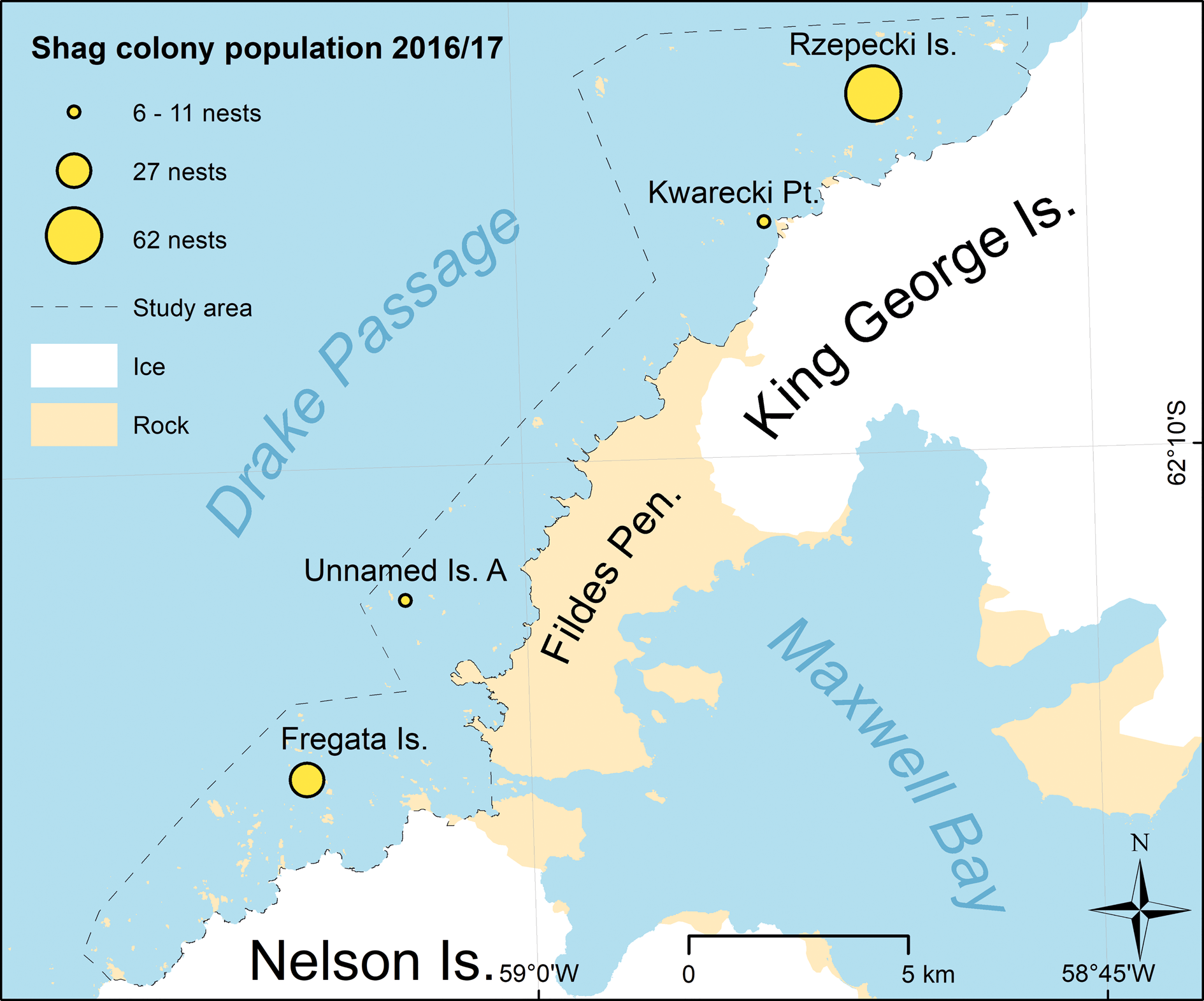
Fig. 11. Positions of the Antarctic shag colonies detected along the coast of Nelson Island and King George Island.
Table V. Comparison of Antarctic shag and chinstrap penguins features visible in aerial images of the study area.

Table VI. Size, date and time of UAV overflights and positions (centre) of the shag colonies in the study area.

Changes in population size and distribution
Comparison with previous surveys showed that the total number of detected colonies stayed the same, though there were changes in the distribution of the smallest colonies (Fig. 12). We found no nests of the colony previously detected at Smilets Point. But we found one small colony at Kwarecki Point that has not been reported before. The total shag population in the survey area increased by a factor of 2.86 compared to previous estimates: 37 in February 1987 and 106 in December 2016. In this period, the population of the two biggest colonies increased but the population of one very small colony hardly changed at all (“Unnamed Island-A”) and in one colony decreased to zero.

Fig. 12. Change in the distribution and abundance of Antarctic shag colonies from breeding season 1986/87 (Shuford & Spear Reference Shuford and Spear1988) to 2016/17 (this study)
There were also major fluctuations in the number of nests at Fregata Island, the only colony with data of three different seasons available. Here, the number of nests increased by a factor of 10 from breeding season 1986/87 to 1989/90 and decreased again by a factor of three in season 2016/17 (see Table VII).
Table VII. Changes in nest numbers with previous counts in the study area.

a Estimated by dividing the number of adults by 1.5 and rounding up the result.
Discussion
Colony characteristics
All colony characteristics we describe are based on the analysis of only four colonies in one region. Though desirable for comparison, very few UAV images are available of other colonies. We were able, however, to compare our results with UAV images of the colony at Turret Point (Korczak-Abshire et al. Reference Korczak-Abshire, Zmarz, Rodzewicz, Kycko, Karsznia and Chwedorzewska2019), Harmony Point (Oosthuizen et al. Reference Oosthuizen, Krüger, Jouanneau and Lowther2020) and Charbier Rock (Korczak-Abshire et al. Reference Korczak-Abshire, Chwedorzewska, Karlsen and Zmarz2017). These UAV images show similar characteristics to those of the colonies analysed in this study like guano colour, nest distance, appearance of adults or colony position. In our study we only had the opportunity to analyse Antarctic shags. Nevertheless, the characteristics we determined for their colonies are likely to be similar to those for colonies of other shag species in the genus Phalacrocorax breeding in Antarctica or sub-Antarctica.
From all the shag colony characteristics analysed, the most distinct features are probably i) the white guano covered areas, contrasting strongly with ii) the black upper part of the adult birds, which are distributed iii) in a relatively even pattern in the colony. A comparison with Korczak-Abshire et al. (Reference Korczak-Abshire, Zmarz, Rodzewicz, Kycko, Karsznia and Chwedorzewska2019) and Mustafa et al. (Reference Mustafa, Braun, Esefeld, Knetsch, Maercker, Pfeifer and Rümmler2019) shows that these features are even visible in images with a ground resolution of 7 cm under optimal conditions. As these characteristics are very similar to penguin colonies, additional features are needed to distinguish between the two species (Table V).
However, we discovered that the visibility of the guano covered areas changes during the breeding season. Their visibility was greatest when there was no precipitation on the immediately preceding days and when there were no clouds at the time of the flights. A possible reason for this is that under such conditions soil moisture was low leading to high guano reflectivity. This effect is well known from other soils (Lobell & Asner Reference Lobell and Asner2002). The relatively dry guano-covered ground appears brighter in the images, which increases the contrast with the dark upper part of the adults or with the surrounding materials. Another possible reason is that the erosion (rinse off) of guano during days with relatively high precipitation (Table II) was higher than the deposition of new guano so that the guano cover was thinner and covered less ground. Considering the weather conditions before and during flights, allows the timing of survey flights to be optimized so as to improve detection of shag colonies in aerial imagery. This information will likely also help increase the detectability of colonies of Pygoscelis penguins or Antarctic petrels (Thalassoica antarctica) in aerial imagery because these mechanisms are very likely to be the same for all colonial breeding birds in Antarctica which produce extensive guano covered areas.
In our experience of flying bird species in Antarctica the nests of shags are probably the most distinctively visible (see Mustafa et al. Reference Mustafa, Braun, Esefeld, Knetsch, Maercker, Pfeifer and Rümmler2019). Therefore, it is possible to determine the breeding population of shags by detecting the nest itself. This is not always straightforward, however, because counting the exact number of nests can be difficult if weather conditions or the spatial resolution of the aerial images are not optimal.
Adults are easier to detect than are nests. But counting adults does not provide a measure of the abundance of breeding birds in a colony. This is because the attendance of adults at nests is not constant. Sometimes both parents are present, sometimes only one and occasionally both are absent. There are also occasional “floating” adults present that are not breeding. Therefore, adult numbers in a colony change over time (cf. Schuckard et al. Reference Schuckard, Melville and Taylor2015 for New Zealand king shags). A possible solution is to apply a correction factor, as for Pygoscelis penguins (Southwell et al. Reference Southwell, McKinlay, Low, Wilson, Newbery, Lieser and Emmerson2013, Pfeifer et al. Reference Pfeifer, Barbosa, Mustafa, Peter, Rümmler and Brenning2019). However, more data are required on inter-daily and inter-seasonal abundance changes.
Distinction of shag and penguin colonies
This study is the first that defines criteria allowing shag nests to be distinguished from those of penguins in UAV imagery.
If colonies of both species are well separated, they are usually distinguishable with the help of features like the guano colour, minimal nest distance or the shadow of the nests.
The visibility of guano changes during a season. Earlier in the season the guano is less visible because less has accumulated on the ground (see Mustafa et al. Reference Mustafa, Esefeld, Grämer, Maercker, Rümmler and Pfeifer2017). A further problem arises later in the season when the penguin chicks start to leave their nests. Distinguishing between colonies of the two different species then becomes more difficult as penguin chicks could walk into shag colonies and between the shag nests. Telling the two apart is likely to be easier, however, when penguin chicks form crèches if they move closer to the shoreline and so further away from the higher lying shag nests.
In areas where shag and penguin colonies overlap, detection of nests can be very difficult if conditions are sub-optimal, e.g. the nest shadow or the differences in guano colour are not visible. For such areas, images with a ground resolution of at least 1.5 cm are required before it is possible to detect distinct direct features of shag nests or individuals like the white upper back, the long neck or the nest edge. But even then, these features are visible only at about a third of the nests or adults (Fig. 9). Thus, reliable detection of all shag nests in a mixed shag-penguin colony is often difficult. In our study, we imaged mixed-colonies (Rzepecki Islands and Kwarecki Point) under optimal weather conditions. In consequence, our counts are reasonably accurate (< 5% accuracy).
To acquire such very high-resolution imagery, the flight height has to be low (e.g. 45 m with the MAPIR Survey-2 RGB camera to achieve 1.5 cm GSD) or the focal length of the lens has to be long. However, both these requirements reduce the ground coverage and, in consequence, more flight time is needed to cover the same area than with higher flight heights or shorter focal length lenses. Therefore, we suggest a two-stage survey for unknown bird colonies. The first stage is to cover the whole area from a relatively high flight height to detect colonies, measure their spatial distribution and collect precise height data for the colony area, which are essential for low level flight planning. The second stage is to cover from low altitude only those colonies where the initial image quality was insufficient for nest detection. Thus, under this scheme, low flights for obtaining high resolution images are carried out only where needed. In this way, overflights at low altitudes are reduced to a minimum so avoiding unnecessary disturbance to wildlife (Mustafa et al. Reference Mustafa, Barbosa, Krause, Peter, Vieira and Rümmler2018, Harris et al. Reference Harris, Herata and Hertel2019). The only available study on the disturbance of shags by UAVs indicates that flight heights down to 25 m by a multirotor UAV only cause a slight response in imperial shags (Leucocarbo atriceps; Weimerskirch et al. Reference Weimerskirch, Prudor and Schull2018). However, for this species there are no studies on the possible impact of fixed-wing UAVs. These UAVs may have different effects because they are similar in shape to predators such as brown skuas (Catharacta antarctica lonnbergi). Further experiments to reveal the possible disturbance level are therefore necessary.
Distribution and abundance
This study provides the first survey for unknown shag colonies with a UAV and covered a significant part of the shag colonies in the region. We surveyed 50% (3 of 6 colonies) of the known shag colonies of King George Island including the biggest colony of King George Island. Also, one of in total three colonies known at Nelson Island was covered by the UAV flights. This 30 km long coastal area shows a relatively high density of shag colonies and high abundance. Together with the colony at Harmony Point (69 nests in 2018; Oosthuizen et al. Reference Oosthuizen, Krüger, Jouanneau and Lowther2020) 2 km south of the study area (see Fig. 1), more than 1% (175 nests) of the total Antarctic shag population is breeding in the area (Schrimpf et al. Reference Schrimpf, Naveen and Lynch2018). This fact qualifies this coast for designation as an important bird area (IBA; Harris & Woehler Reference Harris and Woehler2004).
Whenever possible we conducted the flights under good weather conditions (sunny, low precipitation before the flights) or applied a low flight altitude to obtain images with a very high ground resolution (< 2.7 cm GSD). Nevertheless, it is still likely that we overlooked single nests, particularly if these nests were newly built or relatively flat and therefore not showing the typical characteristics. It is also possible that single nests were counted although there was no nest. This is possible in cases where an adult was resting for a long time on a nest-sized-rock. This would look like an adult sitting on a nest with a false nest shadow and a guano ring. Taking all this into account we estimate that the accuracy of our counts is better than 5% (see Woehler Reference Woehler1993). This estimate is supported by the low range of 1 nest for the three individual observers-counts. For a better assessment of the accuracy, UAV and ground counts must be compared.
As Schrimpf et al. (Reference Schrimpf, Naveen and Lynch2018) stated, all counts of shag nests (also the counts determined in this study) represent the minimum number of breeding pairs for that particular season, because it is unknown if or to what degree the number of active nests changes during the course of the breeding season e.g. by failed breeders. Therefore, it is unknown how close the number of nests counted at a given time is to the true number of active nests of one season (Schrimpf et al. Reference Schrimpf, Naveen and Lynch2018).
We found evidence that shags seem to prefer breeding close to or within penguin colonies. A possible explanation is that the relatively small shag colonies located close to penguin colonies benefit from cooperative defence against predation. All shag colonies in the study area lie within the foraging grounds of south polar skuas (Catharacta maccormicki; Matthias Kopp personal communication 2019). This species feeds occasionally on eggs, chicks or adult Antarctic shags (Bayes et al. Reference Bayes, Dawson and Potts1964, Casaux & Barrera-Oro Reference Casaux and Barrera-Oro2006). This explanation is supported by the fact that there are numerous other unoccupied islands in the study area that also should offer suitable breeding places for shags but are not colonized by penguins. We found one small colony of solitary breeding shags at “Unnamed Island-A”. A possible reason is that there are no penguin colonies in the vicinity (Pfeifer et al. Reference Pfeifer, Barbosa, Mustafa, Peter, Rümmler and Brenning2019) at sites that are also suitable for shag breeding (e.g. next to cliffs). Nevertheless, more analysis of other colonies in the Antarctic Peninsula is necessary to better understand shag breeding site choice.
Changes in population size and distribution
This survey was only the second after 1986/87 (Shuford & Spear Reference Shuford and Spear1988) in which all shag colonies in the study area were surveyed. This allowed us to detect changes in the distribution and abundance of these shag colonies for the first time. This comparison was difficult because of the absence of precise colony position data from Shuford & Spear (Reference Shuford and Spear1988) and Erfurt & Grimm (Reference Erfurt and Grimm1990). With the help of the accurate position of the shag colonies derived by the UAV flights and on the assumption that established colonies are unlikely to have changed their positions since season 1986/87 or 1989/90, we were able to determine the change in occupied nests for all colonies.
We found a previously unknown shag colony at “Unnamed Island-A”. This colony was not mentioned by Shuford & Spear (Reference Shuford and Spear1988) but it is possible that it was overlooked because of its small size and because its nests are among those of a chinstrap penguin colony.
It should be noted that the calculated changes in the colony population since the 1980s are just estimates of long-term changes because of the following uncertainties.
i) Shuford & Spear (Reference Shuford and Spear1988) counted the total number of adults and we converted these to the number of nests by a fixed ratio that was based on eight observations only (Schrimpf et al. Reference Schrimpf, Naveen and Lynch2018). In addition, it is possible that ground counts underestimate the number of nests because of the difficult accessibility of the sites and the complexity of the terrain (Oosthuizen et al. Reference Oosthuizen, Krüger, Jouanneau and Lowther2020).
ii) The exact date of the count of Erfurt & Grimm (Reference Erfurt and Grimm1990) is unknown and this affects its reliability. As in Pygoscelis penguins (Lynch et al. Reference Lynch, Fagan, Naveen, Trivelpiece and Trivelpiece2009) it is possible that in the number of occupied nests decline over the season because of failed breeders. A count late in the breeding season would therefore be an underestimate of the number of nests.
iii) The reported long-term changes are based on two or three measurements only and are therefore vulnerable to inter-annual variability.
This study is the third, together with Korczak-Abshire et al. (Reference Korczak-Abshire, Zmarz, Rodzewicz, Kycko, Karsznia and Chwedorzewska2019) and Oosthuizen et al. (Reference Oosthuizen, Krüger, Jouanneau and Lowther2020), that shows a recent increase in the numbers of shag nests on the South Shetland Islands. It is still unclear whether these increases are part of a general trend in the South Shetland Islands and more recent data of other colonies is needed. It is possible that the increase of the total population is evidence for an increase in the main prey of shags, demersal-benthic fish (Casaux & Barrera-Oro Reference Casaux and Barrera-Oro2006).
Conclusions
We proved the feasibility of UAVs for surveying unknown shag colonies at remote and difficult to access areas at the Antarctic coast. In the survey we were able to identify three shag colonies on the South Shetland Islands where only the rough position was known. One colony found was previously unknown. We also determined the population size of the colonies for the first time since the 1980s. Combined with the precise position of the colonies this data provides an optimal baseline for future surveys. The comparison with previous estimates revealed that the total population of the colonies probably increased by a factor of 2.86 since the 1980s.
By analysing the data of the four colonies we were able to identify several characteristic features in high resolution aerial imagery. These allow a reliable detection of shag colonies and the count of nests. With the same data we were able define unique features that help in distinguishing shag colonies from breeding chinstrap penguin colonies and nests. We found that it is always possible to distinguish colonies of the two species if the colonies are well separated. In areas, where the colonies overlap, detection of single shag nests is difficult especially if the weather and light conditions are sub-optimal. Under such conditions, very high-resolution images can help but the detection of shag nests in penguin colonies is still difficult. We found that the visibility of the most distinct features that allow shag nest detection, like the guano colour and the nest shadow, are weather dependent. Therefore, timing of the flights is the most crucial factor for counting shag nests in mixed colonies. With this knowledge future aerial surveys can be planned in a more targeted way to increase the probability of obtaining optimal imagery and thus more accurate counts of nests.
Acknowledgements
This research was commissioned by the German Federal Environment Agency and funded by the German Federal Ministry for the Environment, Nature Conservation and Nuclear Safety (UFOPLAN 3716 18 210 0). We thank the crew of the Bellingshausen Station (Russian) for accommodation and technical support during our expedition. We thank Christina Braun and Dr Hans-Ulrich Peter for invaluable support before and during the Antarctic field campaign. Thanks to the developers of ArduPilot, ExifTool, QGIS and R for developing and sharing the open-source software that we used in this study. We also thank Dr Michael Schrimpf and one anonymous reviewer for their feedback and insight on previous drafts of this manuscript. Dr Andrew Davis (English Experience Language Services, Göttingen) edited the text during revision.
Author contributions
OM supervised the project, CP and MCR performed the fieldwork, CP processed and analysed the data, CP designed the figures and wrote the manuscript with input from all authors.
Supplemental material
A Shape-file with position of each Antarctic shag nest with date / time of acquisition and site name will be found at https://doi.org/10.1017/S0954102020000644.


