2.1 General equations for free-surface potential flows

In this section, we derive the general equations governing the motion of an inviscid fluid in the case of a potential flow with a free surface. The problem is solved in a cylindrical coordinate system $(r,\unicode[STIX]{x1D703},z)$ . Denoting by $\unicode[STIX]{x1D6F7}$ the velocity potential which is defined by $\boldsymbol{U}=\unicode[STIX]{x1D735}\unicode[STIX]{x1D6F7}$ , Laplace’s and Bernoulli’s equations apply in the fluid volume and read,

with $P$ the pressure (relative to atmospheric pressure) and $\unicode[STIX]{x1D70C}$ the density of the fluid. We now define the free-surface position by the zero level of the implicit function ${\mathcal{H}}(r,\unicode[STIX]{x1D703},z,t)=h(r,\unicode[STIX]{x1D703},t)-z$ with $h$ the vertical height of the free surface and $z=0$ at the bottom of the tank. The kinematic and dynamic boundary conditions on the free surface can therefore be written as with $\unicode[STIX]{x1D6FE}$ the surface tension and ${\mathcal{C}}$ the curvature of the free surface. In the following, the surface tension will be omitted based upon experimental results by Jansson et al. (Reference Jansson, Haspang, Jensen, Hersen and Bohr2006) which indicate that surface tension does not play a crucial role in the formation of the polygonal shape (at least for a set-up with $R\sim 15{-}20~\text{cm}$ ).

Figure 1. Typical free-surface shapes (2.4c ) obtained for a given fluid volume and increasing values of $\unicode[STIX]{x1D709}/R$ from left to right: $\unicode[STIX]{x1D709}/R\rightarrow 0$ , $\unicode[STIX]{x1D709}/R=0.1$ , $\unicode[STIX]{x1D709}/R=0.3$ , $\unicode[STIX]{x1D709}/R=0.5$ .

2.2 Base flow

As discussed previously, we suppose that the base flow is entirely azimuthal, corresponding to a steady and axisymmetric potential vortex, for which the velocity field can be written as

where $\unicode[STIX]{x1D6E4}$ is the circulation of the flow. The singularity at $r=0$ induces a strong decrease of the pressure near the centre of the tank which leads to the formation of a dry area close to the axis of symmetry (see figure 1). The velocity potential of the base flow and the associated pressure and free-surface height then take the form

with $\unicode[STIX]{x1D709}$ the size of the inner dry area, meaning that solution (2.4) is only valid for $r>\unicode[STIX]{x1D709}$ . For a given volume of fluid, examples of free-surface shapes are shown in figure 1 for various values of $\unicode[STIX]{x1D709}/R$ , and where $\unicode[STIX]{x1D701}=h_{0}(R)$ . The conservation of the volume between the state at rest and the base flow can be written as $\unicode[STIX]{x03C0}R^{2}H=\int _{\unicode[STIX]{x1D709}}^{R}2\unicode[STIX]{x03C0}h_{0}(r)r\,\text{d}r$ . This leads to the following expressions for $\unicode[STIX]{x1D701}$ and $\unicode[STIX]{x1D6E4}$ parametrized by the normalized radius of the dry area $\unicode[STIX]{x1D709}/R$ and the aspect ratio

Note that $\unicode[STIX]{x1D701}/R$ and $\unicode[STIX]{x1D6E4}/(2\unicode[STIX]{x03C0}\sqrt{gR^{3}})$ are both growing functions of $\unicode[STIX]{x1D709}/R$ , hence any of these parameters could be used to characterize the intensity of the vortex. In practice we will present all results in terms of $\unicode[STIX]{x1D709}/R$ as this parameter has a clear geometrical significance, and was already used in Tophøj et al. (Reference Tophøj, Mougel, Bohr and Fabre2013). Note that for application to the rotating bottom experiment, the dimension of the dry radius $\unicode[STIX]{x1D709}/R$ is controlled by the angular frequency of the rotating bottom. A simple model based on conservation of angular momentum was proposed in Tophøj et al. (Reference Tophøj, Mougel, Bohr and Fabre2013) and extended in Fabre & Mougel (Reference Fabre and Mougel2014) to relate these two parameters. We do not develop this argument here, as our goal is not to stick to the specific rotating bottom experiment but to consider the potential vortex model as a more general model which may be relevant to other situations as well.

2.3 Perturbation equations

In order to investigate the stability properties of the potential vortex with a free surface, we introduce infinitesimal perturbations of magnitude $\unicode[STIX]{x1D716}$ with eigenmode form

Note that for the sake of simplicity, the perturbation $p$ has been chosen to have the dimension of a pressure over density to remove $\unicode[STIX]{x1D70C}$ in the following which would only appear with the pressure term. Here, $m$ corresponds to the azimuthal wavenumber and $\unicode[STIX]{x1D714}$ is the complex frequency. Any instability of the base flow is then associated with a positive imaginary part of the frequency, denoted in the following $\unicode[STIX]{x1D714}_{i}=\text{Im}(\unicode[STIX]{x1D714})$ . If at least one mode has a positive growth rate for given values of $(a,\unicode[STIX]{x1D709}/R,m)$ , the base flow is unstable and a pattern having azimuthal shape $m$ is expected to emerge with growth rate $\unicode[STIX]{x1D714}_{i}$ and rotation frequency $\unicode[STIX]{x1D714}_{r}=\text{Re}(\unicode[STIX]{x1D714})$ .

The perturbation equations are obtained by linearizing the set of equations (2.1) around the base state defined in the previous section, subject to the boundary conditions (2.2) together with free slip conditions at the wall of the tank. This leads to the following set of equations

with $h_{0}^{\prime }$ the local slope of the unperturbed free-surface shape, which reads $h_{0}^{\prime }=g_{c}(r)/g$ , where $g_{c}(r)=\unicode[STIX]{x1D6E4}^{2}/(4\unicode[STIX]{x03C0}^{2}r^{3})$ corresponds to the centrifugal acceleration. Here $\unicode[STIX]{x1D6FA}(r)=\unicode[STIX]{x1D6E4}/(2\unicode[STIX]{x03C0}r^{2})$ , ${\mathcal{S}}$ is the resolution domain i.e. $(r,z)\in [\unicode[STIX]{x1D709},R]\times [0,h_{0}(r)]$ and $\unicode[STIX]{x2202}{\mathcal{S}}$ is its border composed of the mean free surface $\unicode[STIX]{x2202}{\mathcal{S}}_{0}$ , the bottom wall $\unicode[STIX]{x2202}{\mathcal{S}}_{1}$ and the lateral wall $\unicode[STIX]{x2202}{\mathcal{S}}_{2}$ . In addition, $\boldsymbol{n}$ is defined as the outward normal to the fluid domain ${\mathcal{S}}$ and the $\unicode[STIX]{x1D735}$ operator is now defined as $\unicode[STIX]{x1D735}=[\unicode[STIX]{x2202}/\unicode[STIX]{x2202}r,\text{i}m/r,\unicode[STIX]{x2202}/\unicode[STIX]{x2202}z]$ .

2.4 Numerical method

The set of differential equations (2.8) is solved by means of a finite element method. For this purpose, we introduce test functions $\unicode[STIX]{x1D719}^{\ast }$ and $p^{\ast }$ associated with $\unicode[STIX]{x1D719}$ and $p$ respectively. The variational formulation of the problem is obtained from (2.8a ) and (2.8b ) under the form

and should be valid for any set of test functions $[\unicode[STIX]{x1D719}^{\ast },p^{\ast }]$ . The contribution $\int _{{\mathcal{S}}}\unicode[STIX]{x0394}\unicode[STIX]{x1D719}\unicode[STIX]{x1D719}^{\ast }r\,\text{d}r\,\text{d}z$ is then integrated by parts leading to $\int _{\unicode[STIX]{x2202}{\mathcal{S}}}[\unicode[STIX]{x1D735}\unicode[STIX]{x1D719}\boldsymbol{\cdot }\boldsymbol{n}]r\,\text{d}s-\int _{{\mathcal{S}}}\unicode[STIX]{x1D735}\unicode[STIX]{x1D719}\boldsymbol{\cdot }\overline{\unicode[STIX]{x1D735}}\unicode[STIX]{x1D719}^{\ast }r\,\text{d}r\,\text{d}z$ with $s$ the curvilinear abscissa along the free surface and $\overline{\unicode[STIX]{x1D735}}$ the complex conjugate of $\unicode[STIX]{x1D735}$ . Border terms are obtained using boundary conditions on $\unicode[STIX]{x2202}{\mathcal{S}}_{0}$ , $\unicode[STIX]{x2202}{\mathcal{S}}_{1}$ and $\unicode[STIX]{x2202}{\mathcal{S}}_{2}$ which are given by (2.8c )–(2.8e ). From the impermeability condition on the walls, contributions corresponding to $\unicode[STIX]{x2202}{\mathcal{S}}_{1}$ and $\unicode[STIX]{x2202}{\mathcal{S}}_{2}$ must be zero. Hence, only the border term associated with the free surface is to be retained. Defining two bilinear operators $A$ and $B$ as

the variational formulation can be written as the generalized eigenvalue problem

with eigenvector $[\unicode[STIX]{x1D719},p]$ and corresponding eigenfrequency $\unicode[STIX]{x1D714}=\unicode[STIX]{x1D714}_{r}+\text{i}\unicode[STIX]{x1D714}_{i}$ , which should be valid for any set of test functions $[\unicode[STIX]{x1D719}^{\ast },p^{\ast }]$ . It therefore allows us to obtain a dispersion relation in the form $\unicode[STIX]{x1D714}={\mathcal{F}}(\unicode[STIX]{x1D709}/R,a,m)$ .

Looking at the symmetries of the problem, we see that if $[\unicode[STIX]{x1D719},p;\unicode[STIX]{x1D714}]$ is a solution then so is $[\bar{\unicode[STIX]{x1D719}},\bar{p};\bar{\unicode[STIX]{x1D714}}]$ , where the bar denotes the complex conjugate. This implies that the eigenvalues will be either pure real (waves) or pairs of complex conjugates (an amplified and a damped mode). This property results from the time-reversal symmetry of the inviscid modelling of the flow used here.

In practice, the problem is discretized by first building a mesh by triangulation of the domain ${\mathcal{S}}$ , and then projecting the unknowns $[\unicode[STIX]{x1D719},p]$ and the test functions $[\unicode[STIX]{x1D719}^{\ast },p^{\ast }]$ onto a basis of P1 elements (linear interpolation between the nodes). The resulting matricial eigenvalue problem is eventually solved using a shift-and-invert method. All these operations are performed using the finite element software FreeFEM $++$ (see Hecht Reference Hecht2012).

3.1 General stability maps

Figure 2. Stability maps in the parameter space $(a,\unicode[STIX]{x1D709}/R)$ for different values of $m$ . Grey levels correspond to normalized growth rate contours ( $\unicode[STIX]{x1D714}_{i}\sqrt{g/R}$ ). A small amount of viscous dissipation is introduced with $C=10^{-4}$ to filter out high-order secondary resonances (see appendix B).

Figure 3. Stability map in the parameter space $(a,\unicode[STIX]{x1D709}/R)$ for $m=2$ (plain lines), $m=3$ (dotted lines) and $m=4$ (no lines). Coloured areas correspond to positive growth rate. The main resonances are shown in blue. A small amount of viscous dissipation is introduced with $C=10^{-4}$ to filter out high-order secondary resonances (see appendix B).

Figure 4. Normalized frequencies $\unicode[STIX]{x1D714}_{r}\sqrt{R/g}$ as a function of $\unicode[STIX]{x1D709}/R$ for $a=0.3$ and $m=3$ . Squares at $\unicode[STIX]{x1D709}/R=0.25$ correspond to mode structures shown in figure 5 (filled symbols) and figure 6 (empty symbols).

Figure 2 displays an important result of our work, namely the mapping of the instability regions in the parameter space $(\unicode[STIX]{x1D709}/R,a,m)$ with $2\leqslant m\leqslant 5$ . White areas correspond to parameter regions in which the potential flow is stable and only neutral waves (with real eigenvalues $\unicode[STIX]{x1D714}$ ) are found. Coloured areas correspond to regions where the flow is unstable, with grey levels indicating the corresponding amplification rate. For all values of the azimuthal wavenumber $m$ considered, it is observed that instability occurs in a number of bands. The band with the higher position in the figures, labelled $(0,0)$ , is often the one with the largest instability region and highest values of the growth rates. These larger bands will be referred as main resonances in the following. Note that in this paper the term resonance denotes a linear instability resulting from interaction between two waves with the same frequency. In addition to these main resonances, a number of secondary resonances are observed for each value of $m$ . The latter consist of thinner bands with lower amplification rates, and are always located at lower values of $\unicode[STIX]{x1D709}/R$ (hence lower values of the vortex intensity $\unicode[STIX]{x1D6E4}$ ) than the main ones. In the figures the secondary resonances are labelled with two integers ( $n_{c},n_{g}$ ). As will be explained in the next subsections, these two integers refer to the numbering of the two waves whose interaction is responsible for the resonance.

For wavenumbers $m\geqslant 6$ , similar results are obtained, but with instability bands becoming narrower and amplification rates becoming weaker. On the other hand the cases $m=0$ and $m=1$ are found to be stable in the parameter range investigated in figure 2 (see appendix A for a description of the waves existing in these cases).

Figure 3 shows a superposition of all the instability regions obtained for $m=2$ to $4$ . Considering only the main resonances, the figure shows the same trends as already presented in Tophøj et al. (Reference Tophøj, Mougel, Bohr and Fabre2013) (see their figure 4b), where instability bands with increasing values of $m$ are successively crossed as the parameter $\unicode[STIX]{x1D709}/R$ (hence the circulation of the vortex) is increased. This trend is also consistent with the fact that, in the rotating bottom experiment, polygonal patterns with an increasing number of corners are successively encountered as the angular velocity of the bottom plate is increased.

Note that in the strictly inviscid case, the number of secondary resonances is theoretically infinite and the corresponding bands get thinner and closer to each other as $\unicode[STIX]{x1D709}/R$ approaches zero. For visual clarity of the results displayed in figures 2 and 3, an ad hoc procedure was employed to filter out these higher-order resonances. This procedure corresponds to the introduction of a small amount of viscosity. It is explained in appendix B, where it is shown that it has a limited effect on the main resonances and the lowest-order secondary resonances for the value of viscosity considered, while it damps the higher-order, less significant secondary resonances. Note that only figures 2 and 3 (and results shown in appendix B) correspond to potential viscous results, all the other results presented in this paper are purely inviscid.

3.2 Wave families

As already stated, the white regions in figure 2 are occupied (in the purely inviscid case) by stable modes with purely real frequencies $\unicode[STIX]{x1D714}$ . These modes actually consist of two families of waves whose interaction is at the origin of the instability mechanism. We first document the structure of these waves.

Figure 4 displays the dimensionless frequencies $\unicode[STIX]{x1D714}_{r}\sqrt{R/g}$ of the eigenmodes as a function of the dimensionless radius of the dry area $\unicode[STIX]{x1D709}/R$ for the particular case $a=0.3$ and $m=3$ . The frequencies are clearly organized along two sets of branches with different trends.

The first kind of branches are characterized by an increase of the frequency with increasing $\unicode[STIX]{x1D709}/R$ . The spatial structure of three different eigenmodes associated with this wave family is shown in figure 5 for the parameters corresponding to the three filled squares in figure 4. As can be seen on the views in a meridional plane, the structure of these modes is mostly concentrated in the region close to the lateral wall of the tank, where the free surface of the base flow is the flattest (see figure 1) as the restoring force acting on the free surface is mostly induced by gravity. These modes are thus recognized as gravity waves. Moreover, figure 5 shows that, at a given $\unicode[STIX]{x1D709}/R$ , the higher the mode frequency is the more complex its spatial structure is, with in particular an increasing number of nodes in the radial direction. In the following, the corresponding branches will be called $G_{n}$ with $n$ the number of nodes along the free surface in the outer region. $G_{0}$ therefore corresponds to the simplest gravity wave structure without clear nodes (figure 5 a).

Figure 5. Example of gravity modes obtained for $a=0.3$ , $m=3$ and $\unicode[STIX]{x1D709}/R=0.25$ (filled squares in figure 4). Velocity potential contours (real part of $\unicode[STIX]{x1D719}\text{e}^{\text{i}(m\unicode[STIX]{x1D703}-\unicode[STIX]{x1D714}t)}$ ) on the free surface as seen from a top view representation in the $r$ – $\unicode[STIX]{x1D703}$ plane (top row) and in a meridional cross-section in the $r$ – $z$ plane (bottom row) where the meridional cut corresponds to the thin radial line in the corresponding top view figure. Levels are uniformly distributed and dashed lines correspond to negative values. All the displayed structures correspond to neutral waves ( $\unicode[STIX]{x1D714}_{i}\sqrt{R/g}=0$ ).

Figure 6. Example of centrifugal modes for $a=0.3$ , $m=3$ and $\unicode[STIX]{x1D709}/R=0.25$ (empty squares in figure 4). Contours and conventions are the same as in figure 5. All the displayed structures correspond to neutral waves ( $\unicode[STIX]{x1D714}_{i}\sqrt{R/g}=0$ ).

The second kind of branches are characterized by a decrease of the frequency with $\unicode[STIX]{x1D709}/R$ . The spatial structures of three eigenmodes located along the three first branches of this family, for parameters corresponding to the empty squares in figure 4, are displayed in figure 6. These modes have a rather different structure, as they are now localized close to the dry area, where the free surface is almost vertical, i.e. where the restoring force acting on the free surface is mostly induced by the centrifugal acceleration. These modes are thus recognized as centrifugal waves. Similar to the gravity waves, branches are associated with a different mode structure and differ by the number of nodes on the free surface. In this case however, more complex structures are found to correspond to smaller frequencies, a trend which can be understood in the shallow-water limit (see appendix C, equation (C 29)). Centrifugal wave branches will be denoted as $C_{n}$ with $n$ the number of nodes along the free surface in the inner region (see figure 6).

Figure 7. Normalized frequencies $\unicode[STIX]{x1D714}_{r}\sqrt{R/g}$ and growth rates $\unicode[STIX]{x1D714}_{i}\sqrt{R/g}$ from global stability as a function of $\unicode[STIX]{x1D709}/R$ for $a=0.7$ and $m=3$ . Along $G_{0}$ branch which is highlighted, black squares correspond to mode structures reported in figure 8.

Figure 8. Evolution of the structure of $G_{0}$ when $\unicode[STIX]{x1D709}/R$ increases for $a=0.7$ and $m=3$ . The corresponding frequency evolution is highlighted in figure 7 and the structures shown here correspond to the black squares on figure 7. Contours and colour conventions are the same as in figure 5.

3.3 Wave interaction

As could be observed in figure 4, at the locations where branches of gravity and centrifugal waves cross, there is a small interval of $\unicode[STIX]{x1D709}/R$ where one can observe wave frequency merging. In such intervals, the waves which have otherwise real frequencies interact. Such interactions result in the formation of a couple of complex conjugate eigenvalues, and therefore to an instability. In this paragraph, we investigate the details of these interactions and the structure of the resulting eigenmodes.

Let us first consider a rather deep-water case corresponding to $a=0.7$ and $m=3$ . Figure 7 displays the frequencies as function of $\unicode[STIX]{x1D709}/R$ . In this case, the real parts (upper plot) shows the same trends as already described in figure 4, with two sets of branches interacting as they cross each other. The imaginary parts (lower plot) confirm the existence of an unstable mode in each of the intervals where the waves interact. As already explained these unstable modes are always associated with their stable counterparts with complex conjugate frequencies, but the latter are not considered any longer. Note that in the upper plot, the crossings leading to instabilities are labelled by two indexes $(n_{c},n_{g})$ corresponding respectively to the numbering of the corresponding branches of centrifugal and gravity waves, respectively.

To investigate how the interaction takes place, let us follow the branch associated with the primary gravity wave $G_{0}$ , which is highlighted in figure 7. Figure 8 displays the structure of the eigenmode at four points along this branch, which corresponds to the square symbols in figure 7. Starting from $\unicode[STIX]{x1D709}/R=0.5$ (figure 8 d) is recognized as the pure $G_{0}$ mode as described in § 3.2, with a structure localized near the upper part of the free surface and zero nodes along the free surface. Progressing backwards along this branch, an interaction with the $C_{0}$ branch is observed for $\unicode[STIX]{x1D709}/R\approx 0.417$ . At this point the structure of the eigenmode (figure 8 c) clearly shows the presence of both a gravity wave with the same structure as in the previous plot, and of a centrifugal wave localized around the lower part of the free surface, with the characteristic structure of the $C_{0}$ branch already displayed, i.e. without any nodes along the free surface. This instability is the one related to the rotating polygons (here a triangle) according to Tophøj et al. (Reference Tophøj, Mougel, Bohr and Fabre2013). Note that the gravity wave and centrifugal wave component display a phase shift of a quarter of wavelength in the azimuthal direction, a characteristic of the instability which will be investigated in more detail in the following. Progressing further towards lower values of $\unicode[STIX]{x1D709}/R$ , the structure reverts to that of the pure $G_{0}$ wave (figure 8 b) until an interaction with the $C_{1}$ branch arises for $\unicode[STIX]{x1D709}/R\approx 0.278$ . At this point, the structure of the eigenmode (figure 8 a) is composed of both the gravity wave $G_{0}$ and the centrifugal wave $C_{1}$ characterized by the existence of one node in the lower part of the free surface.

It is noteworthy that for the rather deep case with $a=0.7$ considered here, the amplification rate associated with the secondary resonance $(n_{g},n_{c})=(0,1)$ is slightly larger than that associated with the main resonance $(n_{g},n_{c})=(0,0)$ . This indicates that some secondary resonances may be strong enough to be observed in the experimental set-up for these rather deep-water cases. For $a=0.7$ , an experimental evidence of secondary resonance $(n_{g},n_{c})=(0,1)$ corresponding to $m=3$ (triangular pattern) will indeed be discussed in § 5. Note however that for a given value of $m$ and $a$ secondary resonances do not necessarily need to overcome the main instability to be experimentally relevant as they appear for different values of parameter $\unicode[STIX]{x1D709}/R$ .

Figure 9. Normalized frequencies $\unicode[STIX]{x1D714}_{r}\sqrt{R/g}$ and growth rates $\unicode[STIX]{x1D714}_{i}\sqrt{R/g}$ from global stability as a function of $\unicode[STIX]{x1D709}/R$ for $a=0.3$ and $m=2$ . Along $C_{0}$ branch which is highlighted, empty squares (respectively stars), correspond to mode structures reported in figure 10 (respectively figure 11).

Figure 10. Evolution of the structure of $C_{0}$ when $\unicode[STIX]{x1D709}/R$ increases for $a=0.3$ and $m=2$ . The corresponding frequency evolution is highlighted in figure 9 and the structures shown here correspond to the black empty squares on figure 9. Only velocity potential contours from the top view representation are shown here. Conventions are identical to figure 5.

Figure 11. Evolution of the structure through the instability $(0,0)$ for $m=2$ and $a=0.3$ (empty stars in figure 9). First row: top view representation for the velocity contours (contours and colour conventions are the same as in figure 5). Second row: free-surface displacement contours (real part of $\unicode[STIX]{x1D702}\text{e}^{\text{i}(m\unicode[STIX]{x1D703}-\unicode[STIX]{x1D714}t)}$ ), white circles indicate the position of the critical radius defined by $r_{c}=\sqrt{m\unicode[STIX]{x1D6E4}/(2\unicode[STIX]{x03C0}\unicode[STIX]{x1D714}_{r})}$ . Third row: free-surface displacements at $r=\unicode[STIX]{x1D709}$ (plain line) and $r=R$ (dashed line) as function of $\unicode[STIX]{x1D703}$ .

Figure 12. Normalized frequencies $\unicode[STIX]{x1D714}_{r}\sqrt{R/g}$ as a function of $\unicode[STIX]{x1D709}/R$ for $a=0.3$ and $m=3$ . The shaded area between dashed lines shows the region where a critical radius is present in the fluid domain, i.e. $\unicode[STIX]{x1D709}<r_{c}<R$ . Upper dashed line corresponds to $\unicode[STIX]{x1D714}_{r}=m\unicode[STIX]{x1D6FA}(\unicode[STIX]{x1D709})$ (critical radius at $r=\unicode[STIX]{x1D709}$ ), lower dashed line corresponds to $\unicode[STIX]{x1D714}_{r}=m\unicode[STIX]{x1D6FA}(R)$ (critical radius at $r=R$ ).

As a second illustration, we now consider a shallow-water case corresponding to $a=0.3$ and illustrate the resonance mechanism for the wavenumber $m=2$ . Figure 9 depicts the real and imaginary parts of the frequency as function of $\unicode[STIX]{x1D709}/R$ in the same fashion as in figure 7. In this case, the most powerful secondary resonances occur along the primary branch of centrifugal wave $C_{0}$ , which is highlighted in the figure. Figure 10 illustrates the evolution of the eigenmode structure as one moves along this branch. For $\unicode[STIX]{x1D709}/R=0.25$ (figure 10 f) we observe the typical shape of the $C_{0}$ centrifugal mode. When decreasing $\unicode[STIX]{x1D709}/R$ to 0.19, a first resonance is encountered with the $G_{0}$ mode, leading to the structure illustrated in figure 10(e). As in figure 8(c), this structure is the superposition of the $G_{0}$ and $C_{0}$ waves, with again a phase shift of a quarter of wavelength in the azimuthal direction between the two components. Moving again downwards along the branch, the structure of the $C_{0}$ wave is recovered (figure 10 d) until a resonance occurs with the $G_{1}$ branch (figure 10 c). The same scenario repeats as $C_{0}$ is recovered again when $\unicode[STIX]{x1D709}/R$ is further increased (figure 10 b) up to a resonance with the $G_{2}$ branch (figure 10 a).

To complete the description of the wave interaction process, figure 11 illustrates the structure of the primary unstable mode for three values of $\unicode[STIX]{x1D709}/R$ corresponding to the lower bound ( $\unicode[STIX]{x1D709}/R=0.17$ ), centre ( $\unicode[STIX]{x1D709}/R=0.19$ ) and upper bound ( $\unicode[STIX]{x1D709}/R=0.21$ ) of the instability interval (as identified by stars in figure 9). This figure allows us to highlight two important features of the wave interaction process. First, as best observed on the evolution of the free-surface displacements at $r=\unicode[STIX]{x1D709}$ and $r=R$ as function of $\unicode[STIX]{x1D703}$ (lower row), the phase shift $\unicode[STIX]{x1D713}$ (defined in figure 11) between the centrifugal wave and gravity wave components of the mode varies with $\unicode[STIX]{x1D709}/R$ . At the lower bound (figure 11 a) the two components are nearly in phase ( $\unicode[STIX]{x1D713}\approx 0$ ). At the centre of the unstable range corresponding to the maximum amplification, (figure 11 b), both waves are in quadrature ( $\unicode[STIX]{x1D713}\approx \unicode[STIX]{x03C0}/(2m)$ ) with the gravity wave leading. At the upper bound just before restabilization (figure 11 c), the two components end up out of phase ( $\unicode[STIX]{x1D713}\approx \unicode[STIX]{x03C0}/m$ ). In figure 11 (bottom row), the free-surface displacement at $r=R$ is multiplied by $10$ for visual clarity. This gives an order of magnitude of the amplitude ratio between both waves and means that the amplitude of the centrifugal wave is more than ten times larger than that of the gravity wave.

The second important feature illustrated in figure 11 is the existence of a critical radius, defined as the location where the angular velocity of the mode $\unicode[STIX]{x1D714}_{r}/m$ equals that of the base flow $\unicode[STIX]{x1D6FA}(r)=\unicode[STIX]{x1D6E4}/(2\unicode[STIX]{x03C0}r^{2})$ , i.e.

This location is displayed by a white circle in the lower plots of figure 11, and is superposed on isocontours of the vertical displacement $\unicode[STIX]{x1D702}$ at the free surface.

The critical radius is found to be located in an intermediate radial region in between radial regions corresponding to gravity and centrifugal waves. In the present case of potential base flow with azimuthal velocity evolving in $1/r$ (and $z$ -independent), the presence of the critical radius in the range $[\unicode[STIX]{x1D709},R]$ means that the global mode is slower than the base flow at $r=\unicode[STIX]{x1D709}$ and faster at $r=R$ .

The fact that instabilities are only possible if gravity and centrifugal waves have nearly the same frequency and have relative velocities with respect to the base flow of opposite sign was already predicted by the Tophøj model which captures only the main resonances. This property actually turns out to be also a necessary condition for secondary resonances. To illustrate this, we display in figure 12 the region in the ( $\unicode[STIX]{x1D709}-\unicode[STIX]{x1D714}_{r}$ ) plane for which a critical radius is present in the range $[\unicode[STIX]{x1D709},R]$ (grey region), superposed on the dispersion relations for the case $a=0.3$ and $m=3$ . This figure confirms that all resonances (main and secondary) effectively occur in a range of frequency where a critical radius is present. Note that outside of this range, interactions between two families of waves are also possible but lead to stable near resonances, meaning that the two branches of neutral waves repel and avoid each other instead of merging and giving rise to an unstable mode. This feature is observed in the lower left corner of figure 12 where the irregular behaviour of several branches can be explained as a series of near resonances between an almost horizontal gravity wave branch and a number of centrifugal wave branches. Note that these features where already captured by the simple Tophøj model. It is indeed a characteristic feature of instability processes resulting from wave interactions (see. e.g. Cairns (Reference Cairns1979)). Such events become more salient in the shallow-water limit presented in the following section.

4.1 Shallow-water approximation

In the shallow-water approximation, the flow is supposed to be vertically confined and the flow properties are weakly dependent upon the vertical coordinate. Thus, we can infer an expression for the potential flow with the form

If $K(r)$ is an order-one function, since $z$ is assumed small with respect to the other dimensions of the problem, the last term in (4.1) is effectively a small correction to an otherwise two-dimensional flow. This ansatz also automatically satisfies the boundary condition (2.8e ) at the bottom. Inserting this expression into (2.8a ) leads at leading order to

where $\unicode[STIX]{x0394}_{2}\equiv (\unicode[STIX]{x2202}^{2}/\unicode[STIX]{x2202}r^{2}+1/r\unicode[STIX]{x2202}/\unicode[STIX]{x2202}r-m^{2}/r^{2})$ is the two-dimensional Laplacian operator. Recognizing that 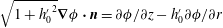$\sqrt{1+{h_{0}^{\prime }}^{2}}\unicode[STIX]{x1D735}\unicode[STIX]{x1D719}\boldsymbol{\cdot }\boldsymbol{n}=\unicode[STIX]{x2202}\unicode[STIX]{x1D719}/\unicode[STIX]{x2202}z-h_{0}^{\prime }\unicode[STIX]{x2202}\unicode[STIX]{x1D719}/\unicode[STIX]{x2202}r$ , where $h_{0}(r)$ is the unperturbed free surface given by (2.4c ), and using (4.1), (2.8d ) and (2.8b ), the kinematic boundary condition (2.8c ) leads at leading order to

Figure 13. Instability map for the main resonance $(0,0)$ and for $m=2,3,4$ and $5$ . Comparison between the numerical solution of the shallow-water equation, (4.4), (contours of normalized growth rate are shown in grey scales) and the instability map obtained from the global stability approach detailed in § 2 (blue zones).

Inserting this latter expression into (4.2) eventually leads to a single ordinary differential equation of the form

with

and

The shallow-water equation, (4.4), can be solved numerically by means of a shooting method and the instability map in the parameter space $(a,\unicode[STIX]{x1D709}/R)$ is shown in figure 13 for $m$ ranging from $2$ to $5$ . Here, only the main unstable interactions are considered and compared to the global stability results. As can be observed in figure 13, the shallow-water model captures the main features of the instability map. In particular, the instability appears as successive bands in the parameter space with an important influence of $\unicode[STIX]{x1D709}/R$ . While the global stability highlights a clear dependence of $a$ on unstable regions, the shallow-water approximation only shows a dependence of the growth rate of the instability. However, the obtained unstable regions and growth rates predicted by the shallow-water model perfectly match the global stability results for small $a$ (see figure 13). The shallow-water limit therefore appears as a good candidate to highlight some features of the instability.

4.2 WKBJ approximation for the shallow-water equation

The fact that the last term of the shallow-water equation, (4.4), is proportional to $m^{2}$ makes it well suited for a WKBJ approach for large $m$ as explained in the appendix C. This kind of large $m$ WKBJ approach has already been used by Ford (Reference Ford1994) to study other velocity profiles of a shallow-water vortex with a free surface. The WKBJ approach allows us to discuss the nature of the solutions of (4.4) based upon the sign of $\unicode[STIX]{x1D6EC}$ . For this discussion, $\unicode[STIX]{x1D714}$ is assumed to be real.

For a given $\unicode[STIX]{x1D714}/m$ , radial positions where $\unicode[STIX]{x1D6EC}(\unicode[STIX]{x1D714}/m,r)<0$ correspond to oscillatory solutions while solutions are evanescent where $\unicode[STIX]{x1D6EC}(\unicode[STIX]{x1D714}/m,r)>0$ . This leads us to introduce the epicyclic frequencies $\unicode[STIX]{x1D714}^{\pm }(r)$ (Le Dizès & Lacaze Reference Le Dizès and Lacaze2005) defined such as $\unicode[STIX]{x1D6EC}(\unicode[STIX]{x1D714}^{\pm }/m,r)=0$ for $r\in [\unicode[STIX]{x1D709},R]$ , along which the WKBJ approximation breaks down. From (4.6), one can obtain

Conversely, for a given $\unicode[STIX]{x1D714}/m$ , radial solutions corresponding to $\unicode[STIX]{x1D6EC}(\unicode[STIX]{x1D714}/m,r)=0$ are the so-called turning points $r_{ti}$ (with $i=1$ or $2$ in the present case) of the WKBJ approximation. Moreover, one can define a critical frequency $\unicode[STIX]{x1D714}_{c}(r)=m\unicode[STIX]{x1D6FA}(r)$ for which the associated mode exhibits a critical radius at location $r$ . For a given solution, the critical radius 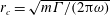$r_{c}=\sqrt{m\unicode[STIX]{x1D6E4}/(2\unicode[STIX]{x03C0}\unicode[STIX]{x1D714})}$ delineates two radial regions where waves travel faster and slower than the base flow as mentioned in the previous section.

Figure 14. Epicyclic frequencies obtained for $a=0.01$ and $\unicode[STIX]{x1D709}/R=0.1$ . Thick lines correspond to the normalized epicyclic frequencies $(\unicode[STIX]{x1D714}^{\pm }/m)\sqrt{R/g}$ given by (4.7), dashed line corresponds to the normalized critical frequency $(\unicode[STIX]{x1D714}_{c}/m)\sqrt{R/g}$ . Grey area corresponds to $\unicode[STIX]{x1D6EC}>0$ (evanescent behaviour), white areas to $\unicode[STIX]{x1D6EC}<0$ (oscillatory behaviour). The inset shows a magnification near $r=\unicode[STIX]{x1D709}$ .

Figure 14 shows the epicyclic frequencies together with the critical frequency as a function of $r/R$ for $a=0.01$ and $\unicode[STIX]{x1D709}/R=0.1$ . In this figure, oscillatory and evanescent behaviours of the solution correspond to white and grey zones respectively. Note that the $\unicode[STIX]{x1D714}_{c}$ curve lies in the evanescent region. Depending on the value of $\unicode[STIX]{x1D714}/m$ for the mode considered, different radial configurations can be anticipated. In particular, a horizontal line in figure 15(a), which corresponds to a given solution $\unicode[STIX]{x1D714}/m$ , may cross (or not) epicyclic and critical frequency curves. This would indicate a change in the behaviour of the solution (oscillatory versus evanescent) and a change in relative velocity sign between the wave and the base flow respectively. Different configurations of radial structures are obtained here, which are highlighted in figure 15(a) where each configuration is identified by a colour (configurations I, II, III, IV). A sketch of the radial structure of the solution for the different configurations (configurations I, II, III, IV) is shown in figure 15(b–e). These different configurations are now described in more details.

1. (i) Configuration I: $\unicode[STIX]{x1D6EC}<0$ for all radial positions and no critical radius. The spatial structure of the associated mode corresponds to the one shown in 15(b). For this purely oscillatory configuration, we do not expect to find two well-separated wave families.

2. (ii) Configuration II: $\unicode[STIX]{x1D6EC}$ changes sign twice along the radial direction and no critical radius. In this case, two oscillatory zones are present and separated by an evanescent zone. This corresponds to figure 15(c). The oscillatory area in the neighbourhood of $\unicode[STIX]{x1D709}$ is associated with centrifugal waves while the oscillatory area close to the external cylinder corresponds to gravity waves. As will be seen these two wave families can be clearly distinguished due to the existence of the evanescent spacial separation.

3. (iii) Configuration III: $\unicode[STIX]{x1D6EC}$ changes sign twice along the radial direction and a critical radius is present. In this case, two oscillatory zones are present and separated by an evanescent zone which now includes a critical radius (figure 15 d). This configuration will be of main importance in the following discussion.

4. (iv) Configuration IV: $\unicode[STIX]{x1D6EC}$ changes sign once along the radial direction and a critical radius can be present. In this case, an oscillatory zone is present close to the inner contact line, while the area enclosing the external cylinder is evanescent (figure 15 e). Note that this configuration could include or not a critical radius. The distinction has not been performed in this paper for simplicity.

Figure 15. (a) Epicyclic frequencies obtained for $a=0.01$ and $\unicode[STIX]{x1D709}/R=0.1$ (same as figure 14) where the different possible configurations depending upon the frequency values are shown in colours. The horizontal lines from top to bottom respectively correspond to $\max (\unicode[STIX]{x1D714}^{+}(r))$ (dotted), $\unicode[STIX]{x1D714}_{c}(\unicode[STIX]{x1D709})$ (dashed), $\unicode[STIX]{x1D714}^{+}(R)$ (plain), $\unicode[STIX]{x1D714}_{c}(R)$ (dashed), $\unicode[STIX]{x1D714}^{-}(R)$ (plain) and $\min (\unicode[STIX]{x1D714}^{-}(r))$ (dotted). (b–e) Sketches of the obtained configurations.

Figure 16. Normalized frequencies $\unicode[STIX]{x1D714}_{r}\sqrt{R/g}$ as function of $\unicode[STIX]{x1D709}/R$ for $m=5$ and $a=0.01$ . Superposition of global stability results (black thick lines) and areas corresponding to the different configurations presented in figure 15. Legends and colours conventions are identical to figure 15.

The location of these different configurations are now reported in figure 16 in which non-dimensional frequencies are plotted as a function of $\unicode[STIX]{x1D709}/R$ in the case $m=5$ and $a=0.01$ . These values of $a$ and $m$ have been chosen to satisfy both the shallow-water approximation and the WKBJ approximation, respectively. In figure 16, black lines correspond to the solutions obtained with the linear stability analysis, and the different zones discussed previously from the WKBJ analysis are delimited thanks to $\unicode[STIX]{x1D714}^{\pm }(R)$ , $\min (\unicode[STIX]{x1D714}^{-}(r))$ , $\max (\unicode[STIX]{x1D714}^{+}(r))$ and $\unicode[STIX]{x1D714}_{c}(\unicode[STIX]{x1D709})$ . Eigenmodes exhibit a critical radius if their dimensionless frequency lies in the interval $[\unicode[STIX]{x1D714}_{c}(R),\unicode[STIX]{x1D714}_{c}(\unicode[STIX]{x1D709})]$ , a region delimited by the dashed lines in figure 16. The general picture of the frequency branches from the global stability in this shallow case ( $a=0.01$ ) is found to be qualitatively similar to the one discussed in § 3 ( $a=0.3$ ). In particular, we recover gravity and centrifugal wave branches, as well as resonances and near resonances. It has been verified in figure 16 that wave crossings in region III indeed correspond to resonance leading to instability (at $\unicode[STIX]{x1D709}/R\approx 0.37$ , $\unicode[STIX]{x1D714}\sqrt{R/g}\approx 1.2$ for instance), while features where branches seem to cross in region II correspond to near resonances without instability (at $\unicode[STIX]{x1D709}/R\approx 0.14$ , $\unicode[STIX]{x1D714}\sqrt{R/g}\approx -0.5$ for instance). It is worth mentioning that the regions were gravity waves and centrifugal waves coexist and are clearly distinguished, correspond to region II and region III (see figure 16). This is in accordance with the spatial structure obtained from the WKBJ analysis and shown in figure 15(c,d). In region IV, only centrifugal branches are found in agreement with the WKBJ structure shown in figure 15(e). In addition, it can be seen in figure 16 that wave families (gravity and centrifugal) do not coexist in region I.

Once focusing only on regions II and III, it is interesting to note that the nature of the wave interaction, leading to a resonance or a near resonance, respectively, depends on the presence or not of a critical radius in the evanescent region of the mode. We therefore recover the importance of the critical radius introduced in the previous section (see figure 12 for instance).

We conclude that the predicted WKBJ structures are strongly correlated to the global stability results and more precisely to the possible occurrence of instability.

In order to investigate the instability mechanisms in more depth, we now focus on configuration III (corresponding to two wavy regions separated by an evanescent region which includes a critical radius), and use asymptotic matching techniques for  $m\gg 1$ to obtain approximate dispersion relations. Technical details associated with the WKBJ method are reported in appendix C and the obtained dispersion relation corresponds to (C 29). Only the case corresponding to the first centrifugal wave (e.g. $n_{c}=0$ ) is discussed here. In this case (C 29) leads to

with

and

where $W_{12}(\unicode[STIX]{x1D714})$ characterizes the potential barrier separating the oscillatory regions delimited by the two turning points $r_{t1}$ and $r_{t2}$ , and $W_{2R}(\unicode[STIX]{x1D714})$ corresponds to the external oscillatory region associated with gravity waves.

Figure 17. Normalized frequencies $\unicode[STIX]{x1D714}_{r}\sqrt{R/g}$ and growth rate $\unicode[STIX]{x1D714}_{i}\sqrt{R/g}$ in the case $m=5$ and $a=0.01$ . 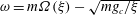Comparison between global stability (thick black lines), numerical solution of the shallow-water equation (thin dotted line approximately on top of the global results), WKBJ results (thick blue line) and the simplified dispersion relations for the first centrifugal wave: $\unicode[STIX]{x1D714}=m\unicode[STIX]{x1D6FA}(\unicode[STIX]{x1D709})-\sqrt{mg_{c}/\unicode[STIX]{x1D709}}$ (open squares) and gravity waves: 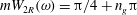$mW_{2R}(\unicode[STIX]{x1D714})=\unicode[STIX]{x03C0}/4+n_{g}\unicode[STIX]{x03C0}$ with $n_{g}=0,1,2$ (filled squares).

Solutions of (4.8) are compared to the numerical solutions of (4.4) and global stability results for $a=0.01$ and $m=5$ in figure 17. From this figure, it can be seen that the main features of the instability are well captured by the WKBJ approach although the position of unstable resonances and associated growth rates are not perfectly reproduced. In addition, figure 17 also shows the solutions corresponding to $D_{c}(\unicode[STIX]{x1D714})=0$ and $D_{g}(\unicode[STIX]{x1D714})=0$ , which fall on top of the solutions of the complete dispersion relation (4.8) except close to resonances, and are recognized to correspond to centrifugal and gravity waves respectively. Dispersion relation (4.8) therefore describes two wave families which can interact if there natural frequencies are close. The intensity of the coupling is found to be proportional to $\text{e}^{-2mW_{12}(\unicode[STIX]{x1D714})}$ and vanishes if the evanescent region is large or for large $m$ . This latter trend is in qualitative agreement with results shown in figures 3 and 13 where both the growth rate and the size of the unstable bands are found to decrease with $m$ .

Figure 18. Reflection coefficient ${\mathcal{R}}$ and normalized growth rate $\unicode[STIX]{x1D714}_{i}\sqrt{R/g}$ as function of $\unicode[STIX]{x1D709}/R$ for $m=5$ and $a=0.01$ . WKBJ results.

In addition, the WKBJ theory allows us to compute the reflection coefficient of a wave at a turning point $r_{ti}$ , delimiting an oscillatory solution with an evanescent region (see Billant & Le Dizès Reference Billant and Le Dizès2009; Park & Billant Reference Park and Billant2013, for instance). In the present case for configuration III, the reflection coefficient of the gravity wave at $r_{t2}$ can be obtained and is shown in appendix C to read

This expression shows that ${\mathcal{R}}=1$ if $\unicode[STIX]{x1D714}$ is purely real, but may be different from one otherwise. This can be seen in figure 18, which shows that the reflection coefficient is unity where $\unicode[STIX]{x1D714}_{i}=0$ , and larger than unity for $\unicode[STIX]{x1D714}_{i}>0$ , i.e. for solutions corresponding to either main or secondary unstable resonances. The instability mechanism for both main and secondary resonances is therefore associated with wave over-reflection. This process has already been described in several cases (see Acheson Reference Acheson1976; Lindzen & Barker Reference Lindzen and Barker1985; Takehiro & Hayashi Reference Takehiro and Hayashi1992; Billant & Le Dizès Reference Billant and Le Dizès2009; Park & Billant Reference Park and Billant2013, for instance). The role of the critical radius on the reflection mechanism has been highlighted in these studies and is also found to be crucial in the present case. In addition the link between over-reflected waves and instability is discussed by Takehiro & Hayashi (Reference Takehiro and Hayashi1992) and more recently by Billant & Le Dizès (Reference Billant and Le Dizès2009). It requires configuration of type III, i.e. two wavy regions separated by an evanescent area, as well as an additional boundary (the wall at $r=R$ or the contact line at $r=\unicode[STIX]{x1D709}$ in our case) to reflect back the over-reflected wave and therefore allowing for multiple over-reflections.

This point of view of the instability mechanism in terms of over-reflection comes as a complement of the interpretation of Tophøj et al. (Reference Tophøj, Mougel, Bohr and Fabre2013) in terms of wave interactions involving negative energy waves (Cairns Reference Cairns1979). In both theory the key ingredients consist of two surface waves radially separated by a critical radius.